Ensemble simulation of the Last Glacial Maximum marine biogeochemistry and atmospheric pCO₂ drawdown due to the soft-tissue biological carbon pump

During the Last Glacial Maximum (LGM), atmospheric pCO₂ was approximately 90 ppm lower than in the pre-industrial era. Several hypotheses have been proposed to explain this difference, including changes in nutrient supply, increased iron input to the ocean, reduced air-sea gas exchange due to changes in sea-ice coverage, and variations in overturning circulation strength driven by differences in wind stress and atmospheric moisture diffusivity. Current modeling approaches that simulate LGM marine biogeochemistry typically use parameter sets calibrated under pre-industrial conditions, assuming that these parameter values are generic and independent of environmental conditions. This could introduce uncertainty due to the imperfect knowledge of the values that should be assigned to the parameters for the LGM environment. The extent to which this uncertainty affects the simulated LGM marine biogeochemistry remains unclear. In this study, we employ an optimality-based variable stoichiometry plankton ecosystem model coupled with a 3D Earth system model to simulate LGM conditions. We conduct sensitivity analyses with 24 combinations of marine biogeochemical (reduced benthic denitrification rate, decreased sedimentary iron input, a higher ${{\mathrm{PO}}_{\mathrm{4}}}^{\mathrm{3}-}$ inventory, and increased atmospheric iron deposition) and physical boundary conditions (changes in wind stress pattern and reduced meridional moisture diffusivity over the Southern Ocean). For each of the 24 combinations, we perform 20 simulations using 20 biogeochemical parameter sets selected out of 600 – each calibrated against present-day observations and representing pre-industrial biogeochemistry about equally well – resulting in a total of 480 simulations. We aim to quantify the uncertainty in simulated LGM marine biogeochemistry and atmospheric pCO₂ arising from uncertainties in parameter settings and boundary conditions. Our results show that changes in iron input, including increased aeolian dust deposition and decreased sedimentary input, exert the most profound influence on marine biogeochemistry and pCO₂ drawdown. Changes in macro-nutrients alone have limited effects, owing to co-limitation effects and the variable stoichiometry in our model. The impact of physical conditions on biogeochemical tracers varies, depending on the specific biogeochemical settings. We found that the changes in carbon to nutrient ratios in particulate organic matter are positively correlated with the changes in Fe supply, and could amplify the effect of Fe availability on changes in the atmospheric pCO₂. Compared to pre-industrial reference conditions, atmospheric pCO₂ under full LGM conditions decreases by 36 to 58 ppm across the 20 simulations. The spread between the maximum and minimum decrease in simulated glacial pCO₂ is approximately 50 % of the mean decrease (43 ppm). These findings highlight that although the 20 parameter sets similarly reproduce pre-industrial marine biogeochemistry, significant variance remains in the marine biogeochemical and atmospheric pCO₂ responses to LGM forcings.

1 Introduction

The Last Glacial Maximum (LGM) was characterised by substantially lower atmospheric pCO₂, around 90 ppm lower than the pre-industrial (Monnin et al., 2001), making it an important case study for understanding the mechanisms influencing changes in pCO₂, with implications for future climate projections. A robust quantitative understanding of the reduced atmospheric CO₂ is still lacking, and several hypotheses have been proposed to explain the lower atmospheric pCO₂ during the LGM. Those include lower sea surface temperatures and higher solubility of CO₂ (Jaccard and Galbraith, 2012), partly counteracted by reduced ocean volume and increased salinity, changes in orbital parameters (Weaver et al., 1998), a higher global nitrate inventory due to reduced benthic denitrification (McElroy, 1983), and a higher global phosphate inventory driven by enhanced terrestrial erosion (Broecker, 1982; Wallmann, 2010; Wallmann et al., 2016), both associated with sea-level retreat. Other factors include changes in the AMOC (Atlantic Meridional Overturning Circulation) (Muglia and Schmittner, 2015), atmospheric moisture diffusivity (Sigman et al., 2007), reduced air-sea gas exchange due to changes in Antarctic sea-ice cover (Stephens and Keeling, 2000), changes in air-sea disequilibrium of carbon (Khatiwala et al., 2019), and enhanced iron (Fe) input to the ocean (Martin, 1990; Martínez-García et al., 2014). Iron is a critical micro-nutrient for marine phytoplankton, particularly in high-nutrient, low-chlorophyll (HNLC) regions, where its scarcity limits productivity (Martin et al., 1987). Two major sources of Fe to the ocean are atmospheric dust deposition and sedimentary inputs. While atmospheric deposition has long been recognised as a major source of Fe, recent studies have shown that sedimentary inputs could have a much larger impact on the Fe cycle in the global ocean (Tagliabue et al., 2016; Somes et al., 2021).

Model simulations are suitable tools for studying the effects of these factors on marine biogeochemistry and their potential contribution to reduced pCO₂ during the LGM. Models that have been applied to study the LGM range from simple box model approaches (Broecker, 1982; Sarmiento and Toggweiler, 1984) to 3D Earth system models that consider ocean circulation and marine biogeochemical cycles (Bopp et al., 2003; Brovkin et al., 2007; Tagliabue et al., 2009; Somes et al., 2017; Kemppinen et al., 2019; Ödalen et al., 2020; Matsumoto et al., 2020a; Kageyama et al., 2021). The biogeochemical components of these Earth system models contain various representations of marine ecosystems, transport and sinking of particles, and cycling of macro- and micro-nutrients.

The calibration of poorly known parameters is an important part of setting up reliable biogeochemical models. In principle, calibration efforts look for a set of optimal parameter estimates that minimises a metric that quantifies the data-model misfit, such as the root mean square error. Some challenges exist in the optimisation process, particularly for Earth system models that often have to cope with sparse data availability with uneven spatial and temporal distribution (Schartau et al., 2017). Also, the computational cost for spinning up Earth system models is often high, particularly for those with higher functional complexity and higher spatial resolution. In the case of high computational costs, the number of parameter sets for which model solutions can be evaluated is limited and for this reason “optimal” parameters are often chosen pragmatically (Séférian et al., 2016). Apart from the number of possible model runs, the choice of an appropriate metric is also crucial. This choice depends objectively on the available data considered, but it is also subjective with regard to the error model employed (Jolliff et al., 2009; Schartau et al., 2017; Kriest et al., 2020). Calibration becomes particularly challenging when it comes to simulating the LGM: Data-model misfits are usually evaluated for pre-industrial or present-day conditions. To what extent a parameter set calibrated against pre-industrial or present-day observations could similarly well represent the LGM is as yet unknown.

Here we employ an optimality-based variable stoichiometry plankton ecosystem model (OPEM) coupled to the University of Victoria (UVic) Earth system model of intermediate complexity (UVic-OPEM) to simulate LGM marine biogeochemistry and atmospheric pCO₂. The model has been devised employing with variable stoichiometry of particulate organic matter (POM), and it provides a relatively reliable representation of the most important biogeochemical processes in today’s ocean (Pahlow et al., 2020; Chien et al., 2020; Li et al., 2024). In addition, by resolving elemental stoichiometry in UVic-OPEM, it is possible to investigate how elemental ratios of particulate organic matter may have differed during the LGM, and how those differences affect the changes in the atmospheric pCO₂. We conduct sensitivity analyses with 24 combinations of LGM boundary conditions (Table 2), namely biogeochemical (reduced benthic denitrification rate, decreased sedimentary iron input, a higher ${{\mathrm{PO}}_{\mathrm{4}}}^{\mathrm{3}-}$ level, and increased atmospheric iron deposition) and physical (changes in wind stress pattern and reduced meridional moisture diffusivity over the Southern Ocean, Muglia and Schmittner, 2015; Sigman et al., 2007). For each combination, the subset of 20 of the 600 parameter sets was considered that exhibit the best model agreement with the observations, resulting in a total of 480 simulations. The objective of this study is to examine the potential uncertainty in LGM simulations due to the typically employed selection of one specific parameter set calibrated for pre-industrial-climate boundary conditions. We also investigate the effects of variable stoichiometry of particulate organic matter (POM) along with different biogeochemical and physical boundary conditions, on atmospheric pCO₂ and marine biogeochemistry during the LGM. We are particularly interested in identifying uncertainties that might play a role in estimating the pCO₂ difference between the pre-industrial era and the LGM. The biogeochemical mechanisms driving glacial carbon drawdown serve as critical natural analogs for evaluating ocean-based carbon dioxide removal (CDR) strategies. For instance, uncertainties in how the glacial ocean responded to increased dust deposition mirror uncertainties in assessing the efficacy of ocean iron fertilization. Our results may provide insights not only regarding the interpretation of past pCO₂ variations, but also into the effectiveness of potential CDR approaches.

2 Materials and Methods

2.1 The UVic-OPEM Earth system model

The Optimality-based Plankton Ecosystem Model was originally implemented in UVic2.9 (Chien et al., 2020; Pahlow et al., 2020), which has since been updated to UVic2.10 (Mengis et al., 2020) for this study. In the current version, we also apply the temperature-independent mortality that has been used for ordinary phytoplankton to diazotrophs. This modification reduces nitrogen fixation in the Arctic region, where it was considered too high in Chien et al. (2020), but it has only a marginal effect on the global nitrogen distribution and fluxes.

2.2 Model calibration and selection of the best 20 parameter sets

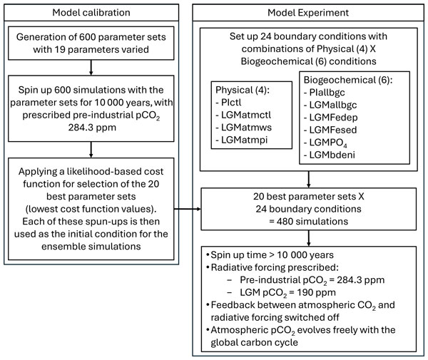
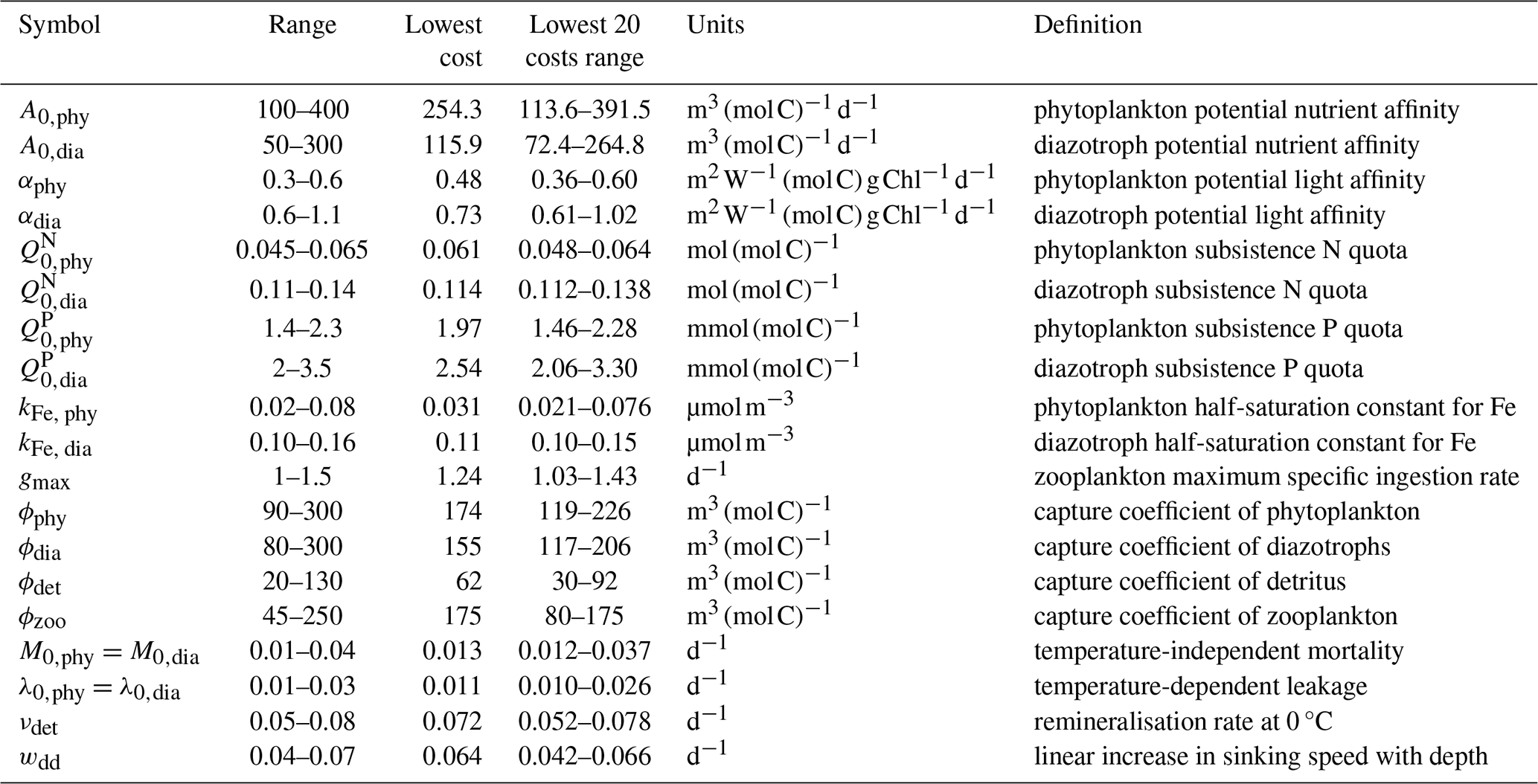
All steps of the experimental design are illustrated in the schematic Fig. 1, with the model calibration and selection of the best parameter sets described in the left hand column. We constructed 600 parameter sets, each representing a unique combination of values assigned to 19 model parameters, including detritus remineralisation rate, the linear increase of sinking velocity with depth, and 17 parameters related to plankton physiology (Table 1). The leakage (implicit remineralisation of organic matter by bacteria) and mortality terms for non-N₂-fixing ordinary phytoplankton and diazotrophs are assumed identical to reduce the number of possible parameter combinations.

Figure 1 Experimental setup and workflow.

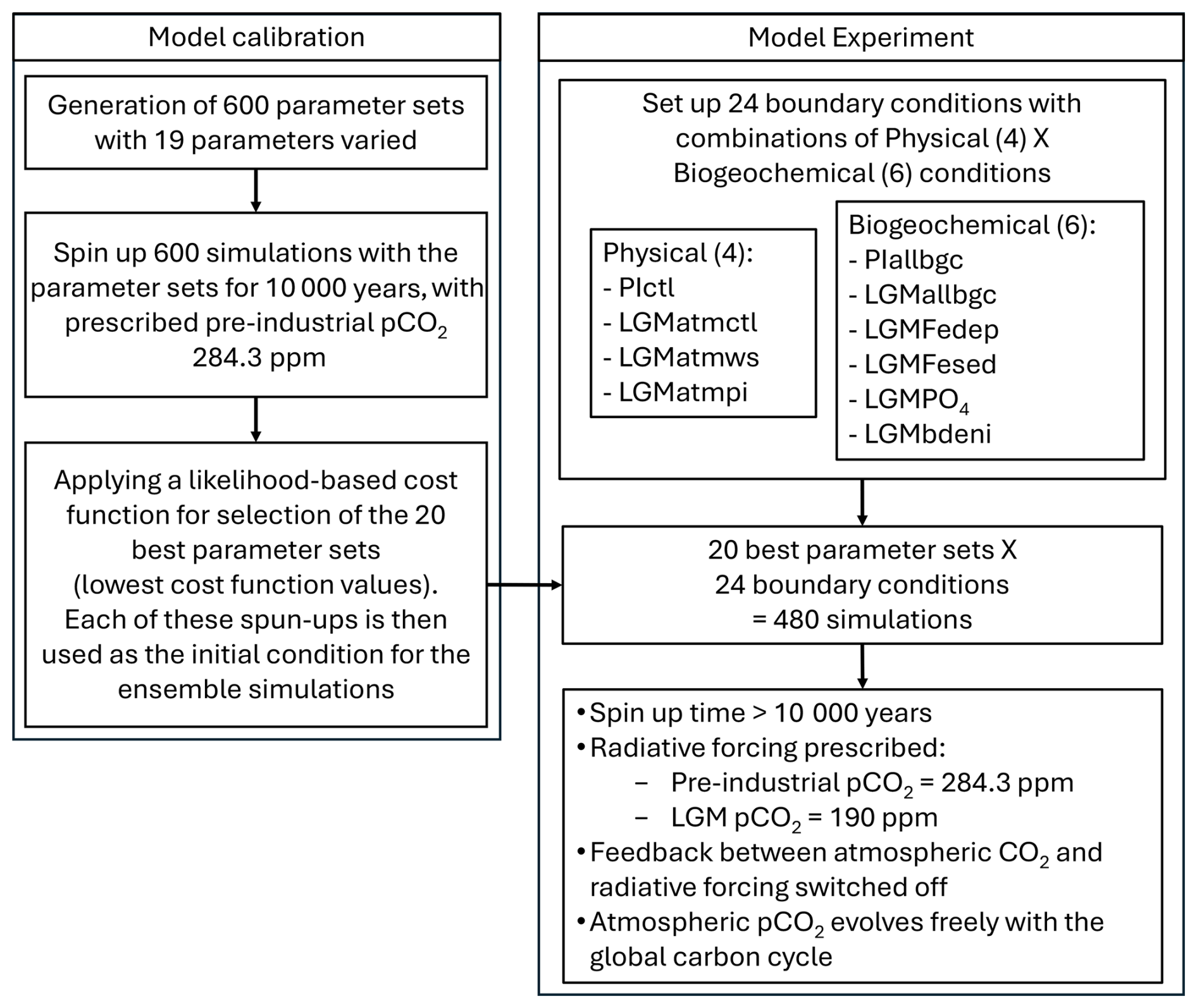
Table 1 Parameter names, variational ranges, the parameter set that yields the lowest cost, the lowest 20 cost parameter sets, units and descriptions. Note that ordinary phytoplankton and diazotrophs share the same temperature dependent leakage rate and temperature independent mortality rate.

The respective 600 simulations were restarted from a previously-calibrated simulation (Chien et al., 2023) and spun up with a prescribed pre-industrial atmospheric pCO₂ of 284.3 ppm for over 10 000 years.

We adopt a likelihood-based cost function for evaluating the biogeochemical model performance (Eqs. 4–9 in Chien et al., 2020). Our cost function considers mismatches in means, and spatial and temporal variabilities of ${{\mathrm{PO}}_{\mathrm{4}}}^{\mathrm{3}-}$, excess nitrate with respect to phosphate (${\mathrm{N}}^{*}={{\mathrm{NO}}_{\mathrm{3}}}^{-}-\mathrm{16}\cdot {{\mathrm{PO}}_{\mathrm{4}}}^{\mathrm{3}-}+\mathrm{2.9}\mathrm{mmol}{\mathrm{m}}^{-\mathrm{3}}$, Gruber and Sarmiento, 1997; Mills et al., 2015), and modified apparent oxygen utilisation (${\text{AOU}}^{*}=\text{AOU}-\mathrm{2}\cdot {{\mathrm{PO}}_{\mathrm{4}}}^{\mathrm{3}-}$), which eliminates the covariation between AOU and ${{\mathrm{PO}}_{\mathrm{4}}}^{\mathrm{3}-}$, in 17 biomes (Fay and McKinley, 2014). Interestingly, most of the best-20 ranges cover about 80 % of the total ranges, except for the four grazing-related parameters ϕs, where the range is “only” about 40 %–60 %. This indicates that parameter values are relatively poorly constrained by currently available observations. Modern observations may include anthropogenic signals, which could bias parameter selection. Thus, we assume here that these effects are small relative to spatial variability and note this as a source of uncertainty we cannot quantify. The 20 best parameter sets (with the lowest cost function values) are employed for analysing model behaviour under pre-industrial (PI) and last-glacial-maximum (LGM) conditions.

2.3 Boundary conditions

We set-up a generic LGM configuration with LGM-specific orbital parameters of the Earth. Besides the different orbital parameters, LGM conditions, including the strength of the AMOC, likely also deviated from the pre-industrial era by a lower moisture diffusivity over the Southern Ocean and a different wind pattern (Muglia and Schmittner, 2015; Muglia et al., 2018). We adopt these forcings from Somes et al. (2017) and Muglia and Schmittner (2015) to investigate their influence on the marine biogeochemistry and carbon cycle. Specifically, meridional moisture diffusivity over the Southern Ocean was reduced by a factor of 2, and the wind stress patterns are from monthly averages of models which have participated in the PMIP3. Compared to pre-industrial conditions, the LGM wind field features an northward shift and intensification of the Southern Ocean westerlies, as well as enhanced trade winds in the tropics and pronounced wind stress anomalies in the North Atlantic (Fig. S1 in the Supplement).

In addition, we configure a 120 m lower sea level compared to PI conditions for the changes in biogeochemical fluxes. The lower sea level was not implemented through an explicit modification of model bathymetry. Instead, it was represented diagnostically in the parameterizations of benthic processes. Specifically, we excluded benthic denitrification and sedimentary Fe input in regions shallower than 120 m relative to the pre-industrial sea level, thereby mimicking the exposure of continental shelves under LGM conditions. This results in reduced benthic denitrification (Somes et al., 2017), reduced sedimentary input of Fe (Tagliabue et al., 2010; Muglia et al., 2017), and a 15 % increase in the ${{\mathrm{PO}}_{\mathrm{4}}}^{\mathrm{3}-}$ inventory (Wallmann et al., 2016), which is conserved in the model. We also include a higher LGM Fe deposition, which was obtained from the LGM dust deposition estimate of Albani et al. (2014, their case C4fn-lgm). Applying a constant iron content of 3.5 % and 1 % solubility of deposited Fe (Kobayashi et al., 2021; Saini et al., 2023) yields an annual Fe deposition of 6.1 Gmol Fe yr⁻¹, which is about four times the pre-industrial flux (Fig. 2). All other physical and biogeochemical processes were computed using the same bathymetry as in the pre-industrial control simulation. This approach allows us to isolate the impact of shelf exposure on benthic fluxes without introducing additional changes to ocean circulation or ecosystem structure that would arise from a fully modified LGM bathymetry.

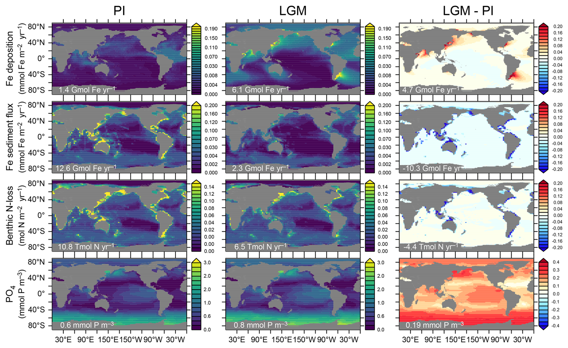
Figure 2 Fe deposition and sedimentary fluxes, benthic denitrification (benthic N–loss), and surface ${{\mathrm{PO}}_{\mathrm{4}}}^{\mathrm{3}-}$ in the PIallbgc and LGM biogeochemical configurations and their differences. PI results are the means of 20 simulations in PIctl_PIallbgc, and LGM Fe deposition, Fe sediment flux, benthic denitrification, and surface ${{\mathrm{PO}}_{\mathrm{4}}}^{\mathrm{3}-}$ are from PIctl_LGMFedep, PIctl_LGMFesed, PIctl_LGMbdeni, and PIctl_LGMPO₄ simulation means. Values on the bottom left of each panel indicate the global annual Fe and N fluxes or ${{\mathrm{PO}}_{\mathrm{4}}}^{\mathrm{3}-}$ concentration.

2.4 Experiment setup

We define four sets of physical and six sets of biogeochemical model configurations, two of which represent pre-industrial climate conditions, PIctl (physical) and PIallbgc (biogeochemical), and the others are different combinations of our generic LGM configuration with PI and LGM boundary conditions (Table 2): LGMatmctl and LGMallbgc refer to the full set of physical and biogeochemical LGM boundary conditions, LGMatmws has PI moisture diffusivity and LGM winds, LGMatmpi has PI moisture diffusivity and winds, and LGMFedep, LGMFesed, LGMPO₄ and LGMbdeni combine PI biogeochemical boundary conditions with one of LGM Fe deposition, Fe sedimentary release, ${{\mathrm{PO}}_{\mathrm{4}}}^{\mathrm{3}-}$ inventory, and benthic denitrification, respectively. These result in a total of 24 (4 physical × 6 biogeochemical) combinations of different physical and biogeochemical boundary conditions. For example, PIctl_LGMallbgc stands for simulations with pre-industrial physics and full LGM biogeochemistry (Table 2). The combination of LGM moisture diffusivity and PI wind stress resulted in a shut-down of the AMOC in the UVic_ESCM and hence is not discussed here. From the calibration stage, we selected the 20 parameter sets that best reproduce present-day observations, each corresponding to a fully spun-up pre-industrial simulation. These simulations serve as initial conditions for the 24 combinations of physical and biogeochemical boundary conditions.

Table 2 Boundary conditions applied in the ensemble simulations for our (A) physical and (B) biogeochemical configurations.

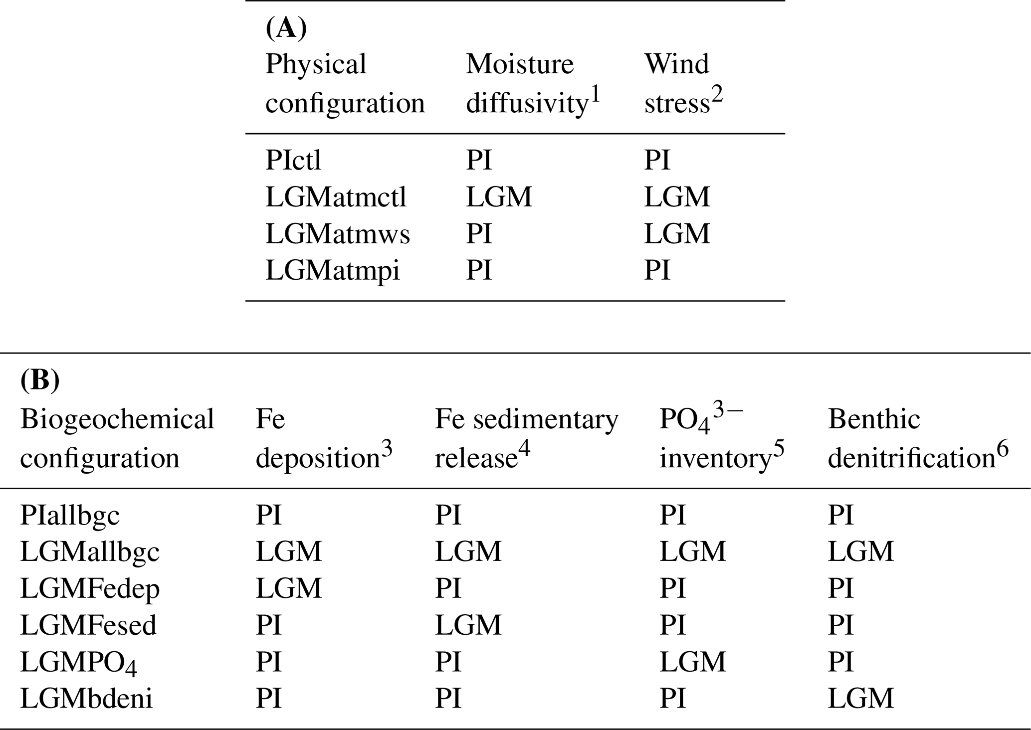
¹ 50 % lower LGM moisture diffusivity over the Southern Ocean in LGM
² LGM wind pattern from Somes et al. (2017); Muglia and Schmittner (2015)
³ ∼4 times higher during LGM
⁴ ∼5 times lower during LGM
⁵ ∼15 % higher during LGM
⁶ ∼40 % lower during LGM.

For each of the 24 configurations, we restarted simulations using the 20 selected parameter sets, resulting in an ensemble of 480 simulations. During the spin-up, radiative forcing was prescribed according to a fixed pCO₂ level (284.3 ppm for PI and 190 ppm for LGM), i.e., the feedback between atmospheric CO₂ and radiative forcing was switched off, while atmospheric pCO₂ was allowed to evolve freely in response to changes in the global carbon cycle.

This physically and biogeochemically coupled but radiatively uncoupled configuration allows us to isolate the effects of boundary conditions on pCO₂, while also accounting for terrestrial carbon responses and ocean–atmosphere carbon exchange. All simulations in the ensemble were spun up for more than 10 000 years under their respective boundary conditions until the marine biogeochemistry approached a steady state. The interannual variability at steady state is negligible because the model simulates a repeating annual cycle (Fig. S2). Therefore, we use the results from the final year of the spin-up simulations for our analysis.

To evaluate whether different physical, biogeochemical, or both conditions result in ensembles that are significantly different from the 20 simulations in PIctl, PIallbgc, or PIctl_PIallbgc, we calculate their p values for each tracer evaluated with Student's t test in R package “Stats”. To understand if changes in individual parameters significantly influence the changes in atmospheric pCO₂ from PIctl_PIallbgc to LGMatmctl_LGMallbgc, we obtain p values using the lm (Fitting Linear Models function) in R package “Stats”.

3 Results

3.1 Model-data misfit costs of all 600 and the selected 20 parameter sets

The 600 parameter sets yield a wide range of model-data misfit costs spanning 2 orders of magnitude (Fig. 3). When the initial 600 pre-industrial simulations are ordered according to increasing cost, the 600 cost values overall show an approximately exponential increase from the low to the high end, with around 8 simulations on both ends deviating from the trend. The 20 simulations with the lowest costs comprise 3.3 % of all simulations, and the cost function values amongst these 20 best are no more than 1.3-fold higher than the overall lowest cost value.

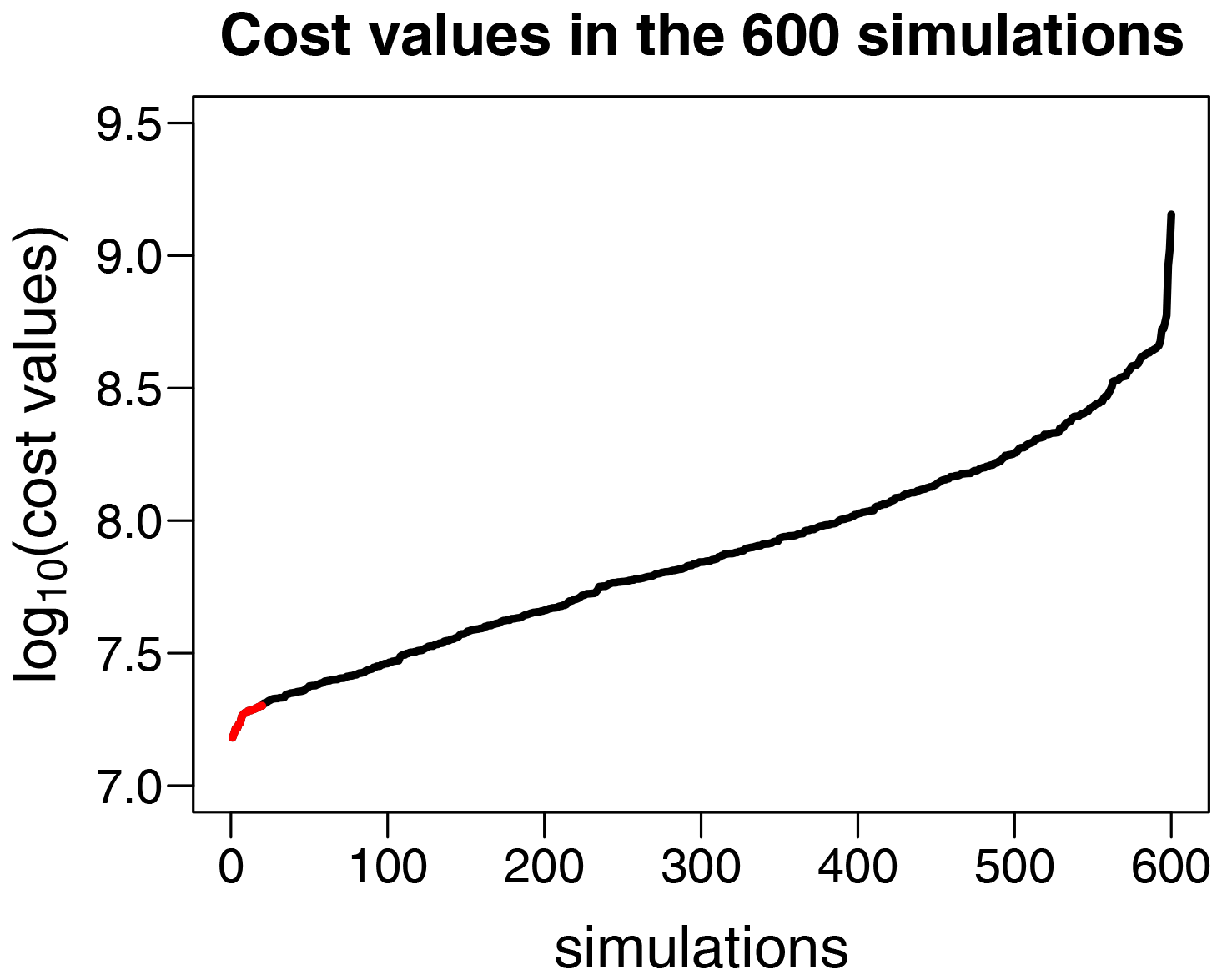
Figure 3 Cost values among all 600 simulations used for calibrating UVic-OPEM ordered from low to high. The red part denotes the 20 simulations with the lowest costs.

Globally-averaged vertical profiles of ${{\mathrm{NO}}_{\mathrm{3}}}^{-}$, ${{\mathrm{PO}}_{\mathrm{4}}}^{\mathrm{3}-}$, O₂, and dissolved inorganic carbon (DIC) in the 20 simulations of PIctl_PIallbgc are compared with observational data from the World Ocean Atlas 2013 (WOA 2013, Garcia et al., 2013a, b) and GLODAPv2 (Key et al., 2015; Lauvset et al., 2016), as well as the original UVic results (Mengis et al., 2020) in Fig. 4. Among the 20 best simulations, ${{\mathrm{NO}}_{\mathrm{3}}}^{-}$ in the upper 500 m of the model is slightly lower than in WOA 2013 but higher than in the original UVic standard solution. In the deep ocean (below 2500 m), simulated ${{\mathrm{NO}}_{\mathrm{3}}}^{-}$ concentrations are generally higher than WOA 2013. The globally-averaged concentrations are close to the WOA 2013 average. ${{\mathrm{PO}}_{\mathrm{4}}}^{\mathrm{3}-}$ concentrations are slightly lower in the upper ocean but higher in the deep ocean than WOA 2013. Our 20 O₂ profiles scatter around the WOA 2013 profile and are lower and closer to the observations than the original UVic simulation (Mengis et al., 2020). The globally-averaged concentrations are about 1.7 % higher than WOA 2013. The DIC profiles are higher than in the original UVic and closer to the GLODAPv2 data. The global mean concentrations are 0.1 % higher than GLODAPv2 on average.

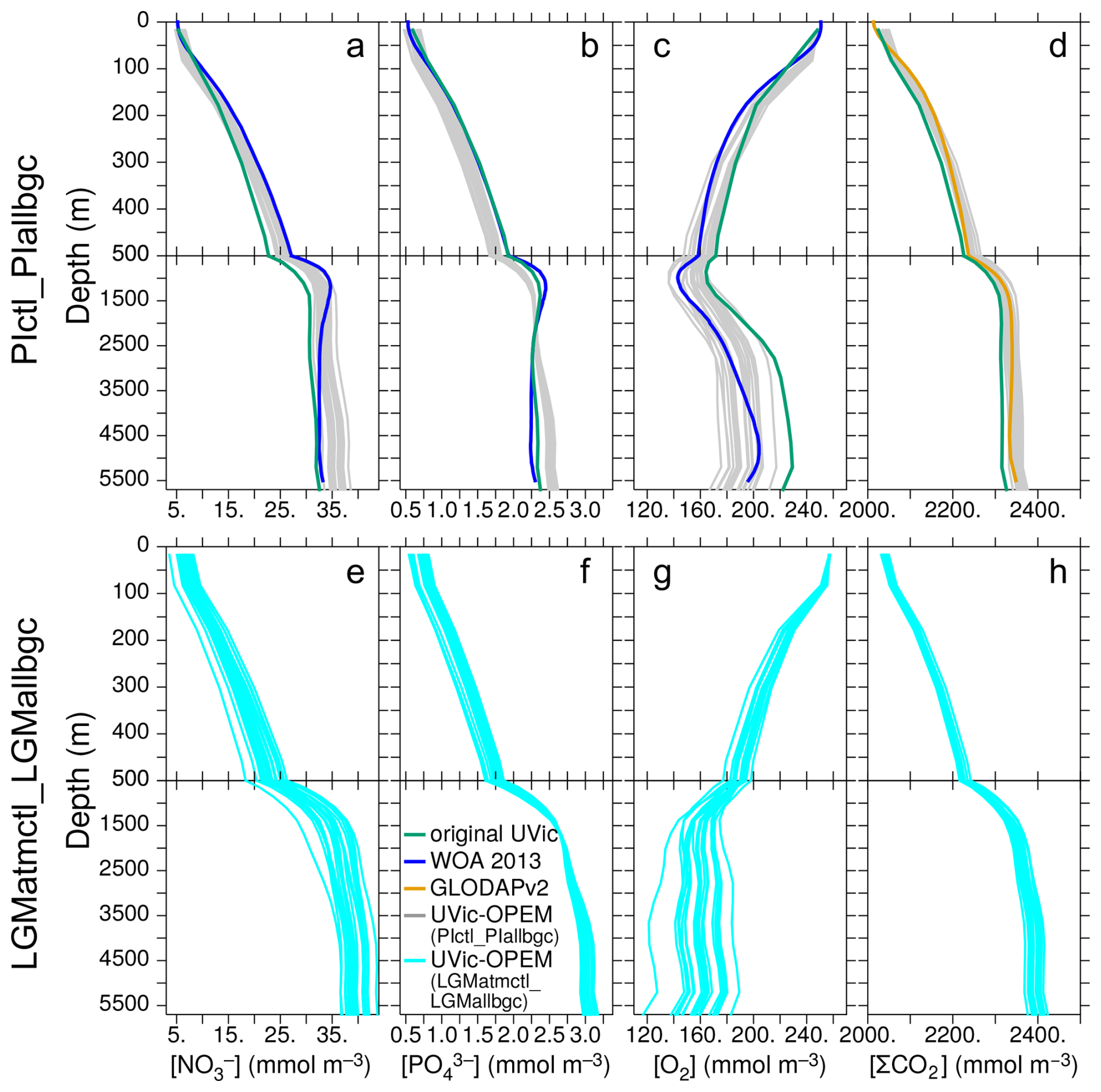
Figure 4 Globally-averaged vertical profiles of ${{\mathrm{NO}}_{\mathrm{3}}}^{-}$, ${{\mathrm{PO}}_{\mathrm{4}}}^{\mathrm{3}-}$, O₂, and DIC (ΣCO₂) concentrations. ${{\mathrm{NO}}_{\mathrm{3}}}^{-}$, ${{\mathrm{PO}}_{\mathrm{4}}}^{\mathrm{3}-}$, and O₂ are considered in the cost function. Black lines are results from the 20 PIctl_PIallbgc simulations, and green lines indicate model results from the original UVic (UVic 2.10, Mengis et al., 2020). Blue and purple lines represent ${{\mathrm{NO}}_{\mathrm{3}}}^{-}$, ${{\mathrm{PO}}_{\mathrm{4}}}^{\mathrm{3}-}$, and O₂ observational data from the World Ocean Atlas 2013 (WOA 2013, Garcia et al., 2013a, b) and ΣCO₂ data from GLODAPv2 (Key et al., 2015; Lauvset et al., 2016), respectively. Light blue lines in the bottom panels show results from the LGMatmctl_LGMallbgc simulations.

Simulated latitudinal patterns of carbon to nitrogen and carbon to phosphorus ratios in particulate organic matter (pC : N and pC : P, respectively) are also compared with observational data (Tanioka et al., 2022). Overall, the modeled ratios show good agreement with observations (Fig. 5), although both the observational data and model results exhibit substantial variability. Modeled pC : N is slightly underestimated at high latitudes (>40°), and overestimated at low latitudes, while pC : P in general is well reproduced across latitudes.

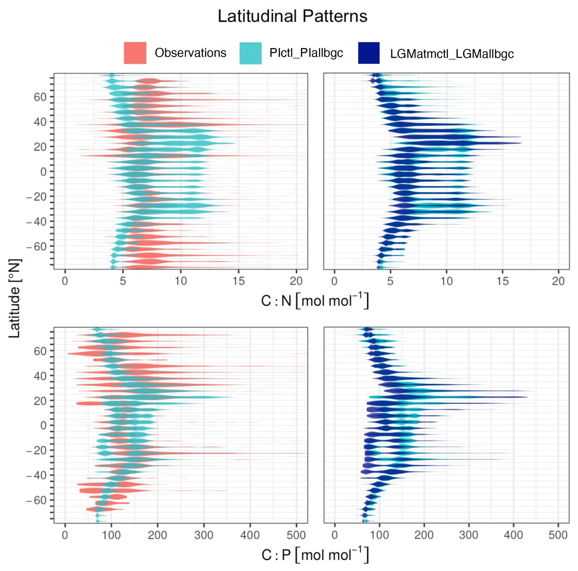
Figure 5 Observed and simulated latitudinal patterns of carbon-to-nitrogen (C : N) and carbon-to-phosphorus (C : P) ratios in particulate organic matter (POM). Observations in the left panels refers to the compilation by Tanioka et al. (2022). Model results represent the mean values from the 20 simulations in PIctl_PIallbgc and LGMatmctl_LGMallbgc.

3.2 Effects of different physical and biogeochemical conditions

We first compare the simulations with LGM and PI physics, each combined with PI biogeochemistry (PIallbgc) to assess the glacial-interglacial changes in global temperature and the Atlantic Meridional Overturning Circulation (AMOC). We then evaluate the effects of different biogeochemical conditions across physical conditions, and vice versa, on marine biogeochemical inventories and atmospheric pCO₂.

3.2.1 Global temperature and ocean circulation

The simulated global surface air temperature in LGMatmctl_PIallbgc is 4.3 °C lower than in PIctl_PIallbgc. Although studies based on proxy records indicate a larger cooling of approximately 5–6 °C (Tierney et al., 2020; Seltzer et al., 2021), the discrepancy is consistent with known limitations of intermediate-complexity models and does not affect the relative differences analysed in this study. In the ocean, the different physical boundary conditions result in distinct thermohaline circulation patterns (Fig. 6). The strength and depth of the maximum value of the AMOC in PIctl_PIallbgc at 26.5° N is 17.82 ± 0.04 Sv at 1100 m, which agrees well with the observational value from the RAPID array of 17.2 ± 0.9 Sv at the same depth (McCarthy et al., 2015). The strength of the maximum AMOC at 26.5° N in LGMatmctl_PIallbgc is reduced by 29 % compared to PIctl_PIallbgc (Fig. 6), which is close to a multi-proxy constrained weakening by 36 % (Pöppelmeier et al., 2023).

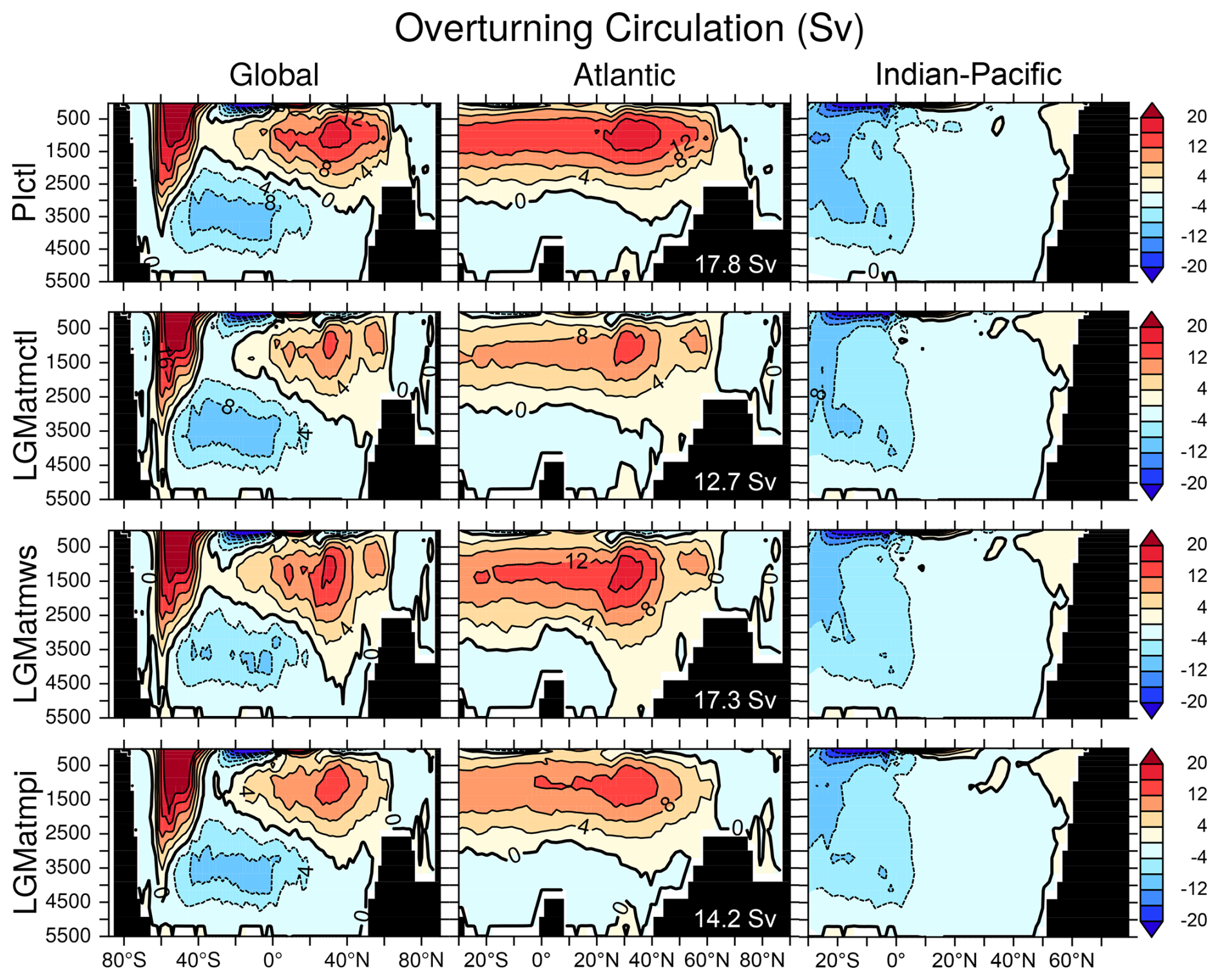
Figure 6 Meridional overturning streamfunction in the Global, Atlantic, and Indian-Pacific Oceans for PIctl, LGMatmctl, LGMatmws, and LGMatmpi, all combined with the PIallbgc biogeochemical configuration. Results are ensemble means over the 20 simulations in each of the configurations. Values in white indicate the strength of maximum AMOC at 26.5° N under each condition.

3.2.2 Dissolved iron

For the pre-industrial control (PIctl) with PI biogeochemistry (PIctl_PIallbgc), the ensemble average (employing the 20 lowest-cost parameter sets) of globally-averaged dissolved Fe (dFe) concentration is 596 ± 14 nmol m⁻³. This value is only slightly lower than the observational estimate of 624 nmol m⁻³ for the modern ocean (Huang et al., 2022) (Fig. S3a and Table S1 in the Supplement). In the *_LGMFedep (*_ stands for all four physical conditions combined with LGMFedep) configurations, the increased Fe input from enhanced dust deposition results in higher dFe concentrations than all other configurations. The average concentration is 15 % higher than in the *_PIallbgc simulations. In the *_LGMFesed simulations, where sedimentary iron fluxes are reduced due to the lower LGM sea level, average dFe concentration is 35 % lower than in the *_PIallbgc simulations, and the lower Fe availability has a strong impact on productivity (−44 %) and export of particulate organic carbon (POC, −39 %). The dFe concentrations in the *_LGMPO₄ and *_LGMbdeni simulations are all similar to those of the PIctl_PIallbgc baseline, indicating that changes in phosphorus and nitrogen cycling have minimal impact on dFe inventories, with Fe availability remaining relatively stable. In *_LGMallbgc simulations, the increased Fe deposition and reduced sedimentary input result in a 1 % decrease in dFe concentration (Fig. S3a and Table S1). Differences in dFe between physical configurations for the same biogeochemistry are much smaller than between biogeochemical configurations (Figs. S3a and S4a). Interestingly, in all LGM physical configurations, dFe is lower than in the corresponding PIctl_* configurations (Fig. S4i). In the model, sedimentary Fe input is associated with the POC flux at the sea floor. Since the POC export declines under LGM conditions due to the lower temperature and lower surface nutrients, sedimentary Fe inputs and consequently the dFe inventories are lower in the LGM than in the PIctl simulations.

Surface dFe (sdFe, 0–50 m) shows similar but more accentuated pattern changes compared to globally-averaged dFe, except that the LGMatmctl_* configurations have higher sdFe than the other LGM physical configurations for the same biogeochemistry (Fig. S3b and Table S1). The overall variation in sdFe is also similar to that of globally-averaged dFe. In *_LGMFedep, the sdFe is 54 % higher than in *_PIallbgc, and this difference is greater than for the globally-averaged dFe (Fig. S4a, b and Table S1). These results highlight the significant role of atmospheric Fe deposition in controlling sdFe concentrations.

3.2.3 Nitrate

The average ${{\mathrm{NO}}_{\mathrm{3}}}^{-}$ concentration in the *_LGMFedep simulations is slightly lower than in *_PIallbgc. Nevertheless, it is significantly lower in the *_LGMFesed simulations than in *_PIallbgc (Figs. S3c and S4c). This strong reduction in *_LGMFesed simulations is likely due to a lower iron availability in *_LGMFesed, which limits N₂ fixation. Indeed, the global N₂ fixation rates are also significantly lower than for *_PIallbgc (Fig. S3k, S5c and Table S2).

The enhanced N₂ fixation due to the greater phosphate availability in *_LGMPO₄ and the reduced benthic denitrification in *_LGMbdeni both produce higher ${{\mathrm{NO}}_{\mathrm{3}}}^{-}$ inventories than *_PIallbgc (Fig. S4c and Table S1, see also Sect. 3.3.2). The ${{\mathrm{NO}}_{\mathrm{3}}}^{-}$ inventories in *_LGMallbgc on average is 2.0 mmol m⁻³ higher than in *_PIallbgc across all physical configurations (Fig. S4c and Table S1). Although the ${{\mathrm{NO}}_{\mathrm{3}}}^{-}$ inventories in *_LGMFesed are substantially reduced due to a lower sedimentary flux of dFe, this negative effect is compensated in *_LGMallbgc by the combined contributions of increased atmospheric Fe deposition (*_LGMFedep), higher ${{\mathrm{PO}}_{\mathrm{4}}}^{\mathrm{3}-}$ inventories (*_LGMPO4), and reduced benthic denitrification (*_LGMbdeni).

In LGMatmctl_LGMallbgc simulations, the average ${{\mathrm{NO}}_{\mathrm{3}}}^{-}$ concentration is 6 % higher than in PIctl_PIallbgc (Fig. S4s and Table S1), and an increase in deep-water ${{\mathrm{NO}}_{\mathrm{3}}}^{-}$ concentrations is also observed (Fig. 4). The increase in ${{\mathrm{NO}}_{\mathrm{3}}}^{-}$ from PIctl_PIallbgc to LGMatmctl_LGMallbgc is lower than the estimates based on paleo proxies (>10 %, Glock et al., 2018; Wallmann et al., 2016; Deutsch et al., 2004). Nevertheless, the increase in 5 out of the 20 individual simulations is larger than 10 %, and the maximum increase reaches 16 %.

In addition to the counteracting effects of *_LGMallbgc on N₂ fixation and denitrification, surface ${{\mathrm{NO}}_{\mathrm{3}}}^{-}$ (s${{\mathrm{NO}}_{\mathrm{3}}}^{-}$) concentrations are also affected by the strength of the ocean circulation and biological utilisation. Therefore, changes in s${{\mathrm{NO}}_{\mathrm{3}}}^{-}$ do not necessarily follow the same pattern as changes in the ${{\mathrm{NO}}_{\mathrm{3}}}^{-}$ inventory. Across all physical configurations, while the ${{\mathrm{NO}}_{\mathrm{3}}}^{-}$ inventory in the *_LGMFedep simulations is only about 7 % lower than in *_PIallbgc, the difference in s${{\mathrm{NO}}_{\mathrm{3}}}^{-}$ is 24 % (Fig. S4c and d). On the other hand, the ${{\mathrm{NO}}_{\mathrm{3}}}^{-}$ inventory in *_LGMFesed is about 30 % lower on average than in *_PIallbgc, but s${{\mathrm{NO}}_{\mathrm{3}}}^{-}$ is only 18 % lower. This apparent inconsistency between changes in ${{\mathrm{NO}}_{\mathrm{3}}}^{-}$ inventory and the surface concentration reflects different responses to changes in iron supply.

3.2.4 Surface phosphate

The mean surface ${{\mathrm{PO}}_{\mathrm{4}}}^{\mathrm{3}-}$ (s${{\mathrm{PO}}_{\mathrm{4}}}^{\mathrm{3}-}$) in PIctl_PIallbgc is 0.62 ± 0.07 mmol m⁻³, which is close to the 0.56 mmol m⁻³ in WOA2013 (Garcia et al., 2013b) (Fig. S3e and Table S1). The average s${{\mathrm{PO}}_{\mathrm{4}}}^{\mathrm{3}-}$ in the *_LGMFedep simulations is about 17 % lower than in the *_PIallbgc simulations, which can be attributed to a higher biological ${{\mathrm{PO}}_{\mathrm{4}}}^{\mathrm{3}-}$ utilisation for elevated dFe supply. The average s${{\mathrm{PO}}_{\mathrm{4}}}^{\mathrm{3}-}$ in the *_LGMFesed simulations, where the sedimentary input of Fe is reduced to about one-fifth compared to *_PIallbgc, is about 62 % higher than in *_PIallbgc, i.e., even higher than in *_LGMPO₄ (Fig. S4e and Table S1, see also Sect. 3.3.3).

3.2.5 Dissolved oxygen

The average dissolved marine oxygen (O₂) concentration in the PIctl_PIallbgc simulations is 179 ± 9 mmol m⁻³. The O₂ inventories in the LGM simulations show considerable variability, with some simulations exhibiting significant deviations from *_PIallbgc (Fig. S4f). O₂ in the *_LGMFedep simulations is 22 mmol m⁻³ lower than in the *_PIallbgc simulations. This decrease is primarily driven by higher oxygen consumption due to the increased remineralisation of particulate organic carbon (POC), a shift that is also consistent with increased water column and benthic denitrification. Conversely, the *_LGMFesed configurations, which feature reduced iron input, result in a remarkable increase by 62 mmol m⁻³ in O₂ concentrations (Fig. S4f).

The *_LGMPO₄ and *_LGMbdeni simulations produce oxygen concentrations only slightly below those in *_PIallbgc. Hence, changes in ${{\mathrm{PO}}_{\mathrm{4}}}^{\mathrm{3}-}$ and ${{\mathrm{NO}}_{\mathrm{3}}}^{-}$ availability alone have limited effects on the O₂ inventory. Overall, the average O₂ in *_LGMallbgc simulations is about 2 % lower than in *_PIallbgc.

Among the LGM physical configurations, O₂ levels are higher in the upper ocean due to a higher solubility under colder conditions, but are lower in the deep water due to a more sluggish circulation (Fig. 4c and g), and the globally-averaged concentrations generally are lower than in the respective PIctl_* simulations. For example, the average concentration for LGMatmctl_* is 2.8 % lower than for PIctl_*. Comparing LGMatmctl_LGMallbgc to PIctl_PIallbgc, global O₂ decreases by 10 mmol m⁻³, which is due to the depletion in the deep water, while the upper ocean concentrations are typically higher (Fig. 4). This agrees with estimated LGM O₂ levels based on paleo proxies (Jaccard and Galbraith, 2012; Anderson et al., 2019) and model simulations (Bopp et al., 2017; Somes et al., 2017). An exception is the *_LGMFesed simulations, where O₂ levels are higher than in the PIctl_* simulations, which indicates a strong coupling with dFe reduction and changes in physical boundary conditions (Fig. S4n).

3.2.6 Dissolved inorganic carbon and atmospheric pCO₂

In the *_LGMFedep simulations, globally-averaged DIC is 3.4 mmol m⁻³ higher than in the corresponding *_PIallbgc simulations (Fig. S4g). In contrast, DIC in the *_LGMFesed simulations is 7.8 mmol m⁻³ lower than in the *_PIallbgc simulations (Fig. S4g). The *_LGMPO₄ and *_LGMbdeni simulations yield DIC concentrations similar to those of *_PIallbgc (Fig. S4g). Our physical LGM configurations yield higher DIC concentrations than the PIctl_* simulations throughout the different biogeochemical configurations (Fig. S4o). Also, the increase in DIC is mostly observed in the deep water (Fig. 4). Further, DIC concentrations within each of the LGM physical configurations are similar, despite the different strength of overturning circulation (Figs. 6 and S4o).

The interglacial-glacial changes in the strength of the solubility pump caused by a reduced temperature, for example, can be obtained by comparing simulated results from PIctl_PIallbgc and LGMatmpi_PIallbgc. The latter shows an average increase of 0.6 % in DIC, which is equivalent to 238 Pg of carbon.

Atmospheric pCO₂ in the biogeochemically coupled but radiatively uncoupled 20 PIctl_PIallbgc simulations is 284.4 ± 0.1 ppm, consistent with the radiatively prescribed 284.3 ppm that was used for the calibration stage (Fig. S3h and Table S1). This indicates equilibrated carbon fluxes between air, land and ocean carbon pools at the end of the spin-ups.

For each of the 4 physical configurations (PIctl, LGMatmctl, LGMatmws, and LGMatmpi, Table 2a), the difference in pCO₂ of employing the biogeochemical LGM forcing conditions with respect to the biogeochemical *_PIallbgc is most pronounced for *_LGMFesed, where pCO₂ increases by 60 ppm, and *_LGMFedep, showing a decrease by 26 ppm (Fig. S4h and Table S1).

The average atmospheric pCO₂ in the physical LGM configurations, LGMatmctl, LGMatmws, and LGMatmpi, are all lower than in the respective simulations for PIctl across all biogeochemical configurations (Figs. S3h and S4p). The pCO₂ in the 20 LGMatmctl_LGMallbgc simulations is 241 ppm on average, which is significantly higher than the LGM atmospheric pCO₂ of approximately 190 ppm recorded in ice cores (Monnin et al., 2001). Thus, the specific mechanisms isolated in these configurations can account for only a portion of the full glacial-interglacial pCO₂ drawdown.

Atmospheric pCO₂ shows different levels of variability among the 20 simulations within each of the biogeochemical configurations. The spread in pCO₂ (i.e., the difference between the maximum and minimum values across simulations) is largest for *_LGMFesed, ranging from 26 to 31 ppm (Fig. S3h). The atmospheric pCO₂ is also influenced by changes in the terrestrial carbon pool. While all LGM physical configurations lead to reduced non-glaciated terrestrial carbon (35 % lower than in PIctl condition) due to changes in radiative forcing, the three LGM atmospheric configurations result in different surface temperature distributions (Fig. S6), which in turn affect the amount of carbon released to the atmosphere and ocean. The combined carbon loss from land and the atmosphere to the ocean in the LGMatmctl, LGMatmws, and LGMatmpi simulations is 251 ± 15, 234 ± 13, and 239 ± 9 Pg C, respectively, relative to PIctl. Of these, changes in atmospheric carbon (1 ppm=2.123 Pg C) account for approximately 30 %, 18 %, and 17 % in the LGMatmctl, LGMatmws, and LGMatmpi simulations, respectively.

3.3 Biogeochemical rate estimates and elemental composition of POM

3.3.1 Marine NPP and POC export

Net primary production (NPP) in PIctl_PIallbgc ranges from 44 to 80 Pg C yr⁻¹, with mean and standard deviation of 64 ± 8 Pg C yr⁻¹ (Fig. S3i and Table S2), in line with observational estimates (36–77 Pg C yr⁻¹, Carr et al., 2006; Honjo et al., 2008; Buitenhuis et al., 2013). Increasing Fe deposition enhances NPP by about 2.8 Pg C yr⁻¹ in the *_LGMFedep simulations when compared with *_PIallbgc. A strong reduction in NPP is associated with the reduced sedimentary Fe flux in the *_LGMFesed simulations, where NPP is about 44 % lower on average than in *_PIallbgc (Fig. S5a). The NPP increases by 1.5 Pg C yr⁻¹ in *_LGMPO₄ and 1.8 Pg C yr⁻¹ in *_LGMbdeni (Fig. S5a). With all biogeochemical conditions combined, NPP in *_LGMallbgc is 11 % lower than in *_PIallbgc. Due to the lower temperature, NPP decreases by 18 % in LGMatmpi_* compared to PIctl_* (Fig. S5i). Compared with the effect of the lower temperature, switching to LGM moisture diffusivity and wind patterns has only relatively small effects on NPP. Compared with LGMatmpi_*, NPP increases by 3 % and 1 % in LGMatmws_* and LGMatmctl_* simulations, respectively. In summary, only *_LGMFesed and LGMatmpi_* affect NPP in a substantial way.

Particulate organic carbon (POC) export shows a similar pattern to that of NPP. The average flux in the PIctl_PIallbgc simulations is 9.2 ± 0.6 Pg C yr⁻¹ (Fig. S3j and Table S2). POC export increases by 9 % for *_LGMFedep and decreases by 39 % for *_LGMFesed, with only small changes in *_LGMPO₄, *_LGMbdeni, and *_LGMallbgc when compared with *_PIallbgc (Fig. S5b). The reduction in POC export due to a cooler climate is 5 % among the LGM physical configurations. This temperature-driven reduction reflects the close coupling between global NPP and export production in the model, while regional changes in iron supply and nutrient utilisation can modulate export production. Proxy-based studies indicate that changes in export production during the LGM relative to the pre-industrial era were spatially heterogeneous with decreases in some low-latitude regions but increases in areas affected by enhanced iron supply, such as the Southern Ocean (Cartapanis et al., 2018; Kohfeld et al., 2005; Toyos et al., 2022).

3.3.2 Marine N₂ fixation and water-column and benthic denitrification

N₂ fixation rates in PIctl_PIallbgc range from 132 to 281 Tg N yr⁻¹ (Fig. S3k), agreeing with observations (223 ± 30 Tg N yr⁻¹, Shao et al., 2023), and inverse-model estimates (126–223 Tg N yr⁻¹, Wang et al., 2019). WC denitrification (water-column N-loss) rates vary strongly among the PIctl_PIallbgc simulations, ranging from 8 to 119 Tg N yr⁻¹, and benthic denitrification rates range from 116 to 169 Tg N yr⁻¹ (Fig. S3l and m), also in line with previous estimates (39 to 66 and 68 to 122 Tg N yr⁻¹ for WC and benthic denitrification rates, respectively, Eugster et al., 2013).

In the model, N₂ fixation is the counterpart of WC and benthic denitrification, thus N₂ fixation equals the sum of WC and benthic denitrification at equilibrium. Across our physical configurations, N₂ fixation increases by 37 % (65 Tg N yr⁻¹) on average in *_LGMFedep simulations compared with *_PIallbgc, due to the extra input of Fe relieving iron limitation of diazotrophs (Fig. S5c). WC denitrification is 197 % (56 Tg N yr⁻¹) higher (Fig. S5d), compensating for most of the increase in N₂ fixation, and benthic denitrification only increases by 5 % (8 Tg N yr⁻¹, Fig. S5e). N₂ fixation drops by 53 % (93 Tg N yr⁻¹) on average in the *_LGMFesed simulations, while benthic denitrification decreases by 43 % (62 Tg N yr⁻¹) and WC denitrification shuts down entirely (Fig. S3l).

In the *_LGMPO₄ simulations, N₂ fixation and the sum of denitrification increase by 5 % (8 Tg N yr⁻¹) compared to *_PIallbgc (Fig. S5c). Benthic denitrification decreases by 31 % (46 Tg N yr⁻¹) on average in the *_LGMbdeni simulations, while WC denitrification increases by 52 % (15 Tg N yr⁻¹), and N₂ fixation is 18 % (31 Tg N yr⁻¹) lower than in *_PIallbgc. In *_LGMallbgc, N₂ fixation and WC and benthic N denitrification decrease by 31 % (55 Tg N yr⁻¹), 22 % (6 Tg N yr⁻¹), and 33 % (47 Tg N yr⁻¹), respectively (Fig. S5c–e).

3.3.3 Elemental composition of POM

The elemental ratios of particulate organic matter (POM) provide insights into nutrient utilisation efficiency and the coupling between carbon, nitrogen, and phosphorus in marine ecosystems. Here we analyse the particulate carbon to nitrogen (pC : N), carbon to phosphorus (pC : P), and nitrogen to phosphorus (pN : P) ratios. The ecological elemental ratios do not follow normal distributions, and we calculate medians of the elemental ratios without biomass weighting in the ocean grid cells that are not covered by ice, rather than mean values to avoid unnecessary bias (Isles, 2020). The global median of surface (0–50 m) pC : N, pC : P, and pN : P in the PIctl_PIallbgc simulations are 8.0 ± 0.5 mol mol⁻¹, 134 ± 8 mol mol⁻¹, and 16.5 ± 0.7 mol mol⁻¹, respectively (Fig. S3n–p and Table S2). When comparing different biogeochemical conditions to *_PIallbgc, the change in globally-averaged pC : N is negatively correlated with the change in s${{\mathrm{NO}}_{\mathrm{3}}}^{-}$ (Figs. S4d and S5f). Nevertheless, the pC : N is lower despite lower s${{\mathrm{NO}}_{\mathrm{3}}}^{-}$ in *_LGMFesed (Tables S1 and S2) because of the shrinking area with low s${{\mathrm{NO}}_{\mathrm{3}}}^{-}$, caused by low ${{\mathrm{NO}}_{\mathrm{3}}}^{-}$ utilisation under strong iron limitation, such as the South Pacific Ocean, and hence the area with high pC : N also becomes smaller (Fig. S7). In general, pC : N in the model is mainly affected by two factors. One is the Fe limitation of carbon fixation and ${{\mathrm{NO}}_{\mathrm{3}}}^{-}$ utilisation, and the other is the supply of ${{\mathrm{NO}}_{\mathrm{3}}}^{-}$ to the surface ocean.

The relation between pC : P and surface ${{\mathrm{PO}}_{\mathrm{4}}}^{\mathrm{3}-}$ (s${{\mathrm{PO}}_{\mathrm{4}}}^{\mathrm{3}-}$) is similar to the relation between pC : N and s${{\mathrm{NO}}_{\mathrm{3}}}^{-}$ (Fig. S3o). Since the ${{\mathrm{PO}}_{\mathrm{4}}}^{\mathrm{3}-}$ inventory is constant in the model, s${{\mathrm{PO}}_{\mathrm{4}}}^{\mathrm{3}-}$ is largely affected by the supply of dFe. In LGMatmctl_LGMallbgc simulations, s${{\mathrm{PO}}_{\mathrm{4}}}^{\mathrm{3}-}$ and s${{\mathrm{NO}}_{\mathrm{3}}}^{-}$ are higher than in the PIctl_PIallbgc (Fig. S4t and u), and the pC : N and pC : P are generally lower, particularly in low latitude regions where the surface nutrients are higher (Fig. 5). In *_LGMFesed simulations s${{\mathrm{PO}}_{\mathrm{4}}}^{\mathrm{3}-}$ increases with lower iron supply. As a result, pC : P in *_LGMFesed simulations decreases by 54 mol mol⁻¹ (39 %), while pC : N decreases by only 1.3 mol mol⁻¹ (16 %) when compared with *_PIallbgc (Fig. S5g and f).

Compared with *_PIallbgc, the average s${{\mathrm{PO}}_{\mathrm{4}}}^{\mathrm{3}-}$ increases by 31 % in *_LGMPO₄ and by 62 % in *_LGMFesed. Moreover, the effects of Fe limitation on carbon fixation and nitrogen assimilation are weaker in *_LGMPO₄ than in *_LGMFesed. As a result, pC : P and pN : P decrease by 10 % and 6 %, respectively, in *_LGMPO₄, which is substantially smaller than the reductions found in *_LGMFesed.

Due to the stronger increase in pC : P relative to pC : N, pN : P decreases by 31 % in *_LGMFesed (Fig. S5h), while other biogeochemical LGM configurations have smaller effects. Physical boundary conditions also contribute to the changes in the elemental ratios of POM via effects on s${{\mathrm{NO}}_{\mathrm{3}}}^{-}$ and s${{\mathrm{PO}}_{\mathrm{4}}}^{\mathrm{3}-}$. The pC : N and pC : P in general are highest for LGMatmctl and lowest for PIctl and LGMatmws, and pN : P is highest in the LGMatmctl configuration (Fig. S5n–p).

4 Discussion

4.1 Physical boundary conditions and ocean circulation

The UVic-ESCM responds to the transition from pre-industrial to LGM wind stress with an increased northward salt transport in the North Atlantic, which enhances surface salinity and density, thereby strengthening North Atlantic Deep Water formation while intensifying and deepening the AMOC. In contrast, reduced atmospheric moisture diffusivity decreases meridional freshwater transport to the Southern Ocean, leading to changes in surface buoyancy and enhanced vertical stratification. This suppresses deep water formation, particularly of Antarctic Bottom Water, which weakens the deep return flow, resulting in a weaker and shallower global overturning circulation, including the AMOC (Sigman et al., 2007; Somes et al., 2017). When all LGM physical boundary conditions are applied simultaneously (LGMatmctl_PIallbgc), the maximum AMOC strength at 26.5° N shows a 29 % reduction, and the depth remains similar to pre-industrial conditions (PIctl_PIallbgc).

The model results show only small changes in the MOC of the Indian and Pacific Oceans, with close agreement between LGMatmctl_PIallbgc and PIctl_PIallbgc. This indicates that the effect of the LGM lower surface temperature is almost compensated by the LGM winds and atmospheric moisture diffusivity. As a consequence of the virtual insensitivity of the Indo-Pacific MOC to a switch from pre-industrial to LGM boundary conditions, changes in the global MOC essentially mirror the changes in the AMOC (Fig. 6).

4.2 Effects of biogeochemical boundary conditions on biogeochemistry

Among the four interglacial-glacial changes in biogeochemical boundary conditions investigated, iron supply has the strongest impact on the inventories and fluxes. Clearly, it is the changes in Fe availability within the surface layer that alter iron limitation and affect NPP and POC export (Fig. 7). The lower dFe inventory during the LGM seems in conflict with the general understanding of Fe fertilisation during the LGM (Martin, 1990; Martínez-García et al., 2014). Interestingly, although NPP and POC export are lower in the *_LGMallbgc relative to the *_PIallbgc simulations, the corresponding atmospheric pCO₂ in general is lower as well (Fig. 7 and Table S1). The atmospheric pCO₂ in the *_LGMallbgc simulations is lower compared to *_PIallbgc, and is primarily driven by a spatial redistribution of surface DIC and the associated changes in global air–sea CO₂ fluxes (Fig. S8).

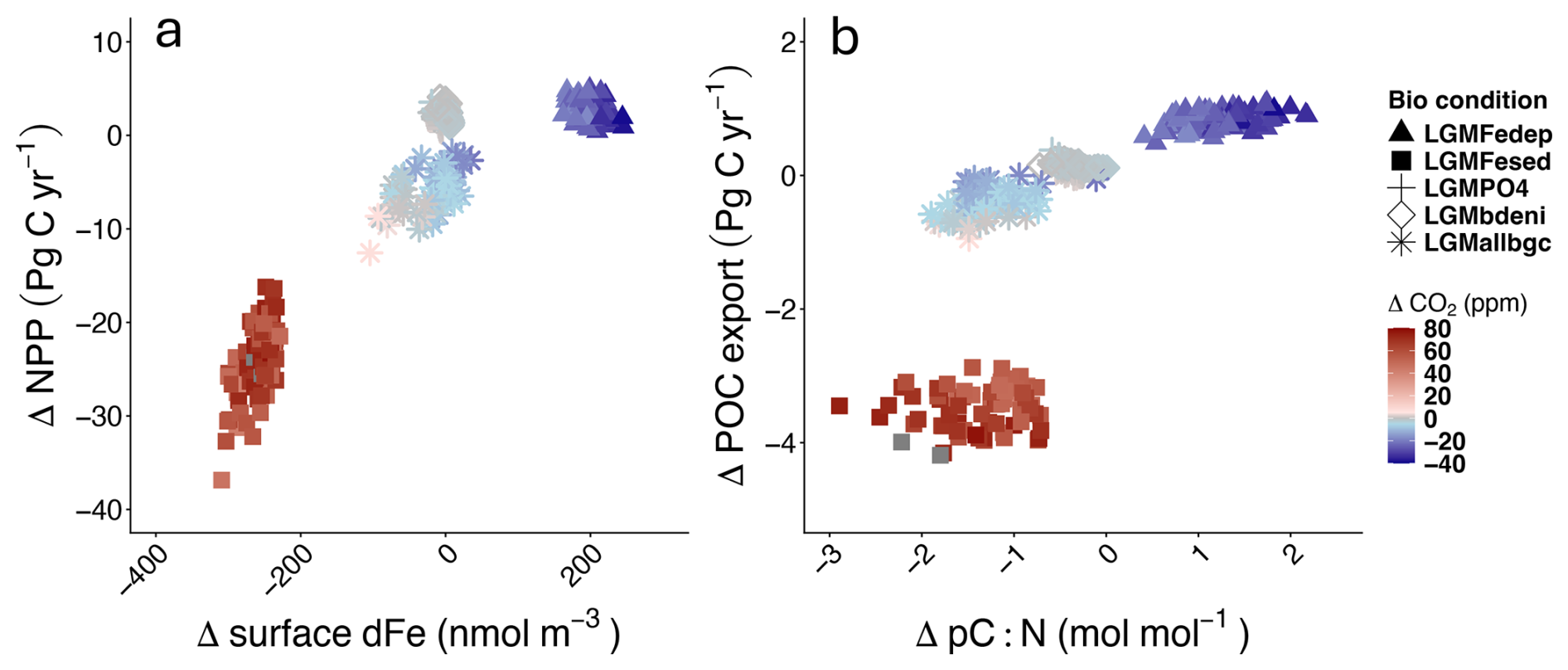
Figure 7 Differences in (a) NPP and surface dFe and (b) POC export and pC : N with respect to default biogeochemical conditions (PIallbgc). Color represents atmospheric pCO₂ and symbols indicate the different biogeochemical configurations. The cluster of points with little deviation from *_PIallbgc simulations is from *_LGMPO4 and *_LGMbdeni simulations.

Glacial-interglacial changes in sedimentary Fe input were not considered in several earlier studies (Somes et al., 2017; Ödalen et al., 2020; Matsumoto et al., 2020a, b; Vollmer et al., 2022). Nevertheless, the strong sensitivity of the biogeochemical inventories and fluxes to changes in sedimentary influx of Fe demonstrates its importance. In our model, the lower glacial sea level leads to a proportional reduction in sedimentary Fe supply from *_PIallbgc to *_LGMFesed (≈80 %, corresponding to a drop of 10.3 Gmol Fe yr⁻¹). This reduction is larger than the increase in atmospheric Fe deposition from *_PIallbgc to *_LGMFedep (4.7 Gmol Fe yr⁻¹), resulting in smaller dFe inventories in *_LGMallbgc.

At first glance, one might expect that the magnitude of sedimentary Fe input in the model is relatively large and that its reduction could therefore be overestimated. However, the simulated sedimentary Fe flux in PIctl_PIallbgc (12.6 Gmol Fe yr⁻¹) falls close to the lower end of estimates from other models (0.6–194 Gmol Fe yr⁻¹, Tagliabue et al., 2016). A recent sensitivity study also shows that a much higher present-day sedimentary Fe release (117 Gmol Fe yr⁻¹) yields a better model-data fit in global and surface dFe distributions (Somes et al., 2021). Assuming that the glacial loss of sedimentary Fe input scales proportionally with the PI baseline due to shelf exposure, our low PI baseline implies that the absolute drop in sedimentary Fe supply (10.3 Gmol Fe yr⁻¹) is a conservative estimate; a higher PI baseline would yield an even larger net Fe deficit relative to the atmospheric supply. On the other hand, a higher PI baseline would also leave a larger absolute amount of sedimentary Fe available during the LGM, which would mitigate the severe ocean-wide iron limitation observed in our simulations. This highlights the critical need to better constrain both the baseline magnitude and bathymetric scaling of sedimentary Fe release when evaluating glacial-interglacial biogeochemical cycles.

While dFe availability affects N₂ fixation, simulations with higher dFe supply and concentrations do not necessarily result in higher ${{\mathrm{NO}}_{\mathrm{3}}}^{-}$ inventories. For example, the average ${{\mathrm{NO}}_{\mathrm{3}}}^{-}$ concentration for *_LGMFedep is 2.0 mmol m⁻³ lower than for *_PIallbgc. This is because changes in Fe supply in our simulations do not only affect N₂ fixation, but can induce changes in denitrification, which in turn depends on the level and consumption of oxygen, in association with the attenuation of the exported particulate organic matter (POM). Two ${{\mathrm{NO}}_{\mathrm{3}}}^{-}$ sinks can occur in the model solutions. One sink is due to the water-column (WC) denitrification, which is affected by WC O₂ supply and consumption via POM remineralisation. The other is benthic denitrification, which is sensitive to the amount of POC reaching the sea floor. Thus, both water column and benthic denitrification are affected by the POM export. The higher Fe supply in the surface ocean increases not only N₂ fixation but also NPP and POM export, thereby promoting both WC and benthic denitrification. The net effect on the ${{\mathrm{NO}}_{\mathrm{3}}}^{-}$ inventory depends on the balance of these counteracting fluxes. Whenever ${{\mathrm{NO}}_{\mathrm{3}}}^{-}$ concentrations are lower in a simulation in *_LGMFedep than in *_PIallbgc, the increase in denitrification is higher than the increase in N₂ fixation at the beginning of the spin-up, because the increase in N₂ fixation due to a higher Fe supply is hampered by the supply of the other limiting macronutrient, ${{\mathrm{PO}}_{\mathrm{4}}}^{\mathrm{3}-}$. Under such conditions, the model yields results with a lower ${{\mathrm{NO}}_{\mathrm{3}}}^{-}$ inventory once the simulation reaches equilibrium despite an increase in N₂ fixation. This explains that while global N₂ fixation in *_LGMFedep simulations is higher than for *_PIallbgc (Fig. S5c and Table S2), the ${{\mathrm{NO}}_{\mathrm{3}}}^{-}$ inventories in *_LGMFedep show a mixed response (Fig. S4c and Table S1).

Since the global ${{\mathrm{PO}}_{\mathrm{4}}}^{\mathrm{3}-}$ inventory is fixed in the model, the higher ${{\mathrm{PO}}_{\mathrm{4}}}^{\mathrm{3}-}$ levels in the LGMPO₄ configuration directly translate into higher surface concentrations. In the *_LGMPO₄ simulations, s${{\mathrm{PO}}_{\mathrm{4}}}^{\mathrm{3}-}$ on average is about 31 % higher than in *_PIallbgc, which is more than the 15 % increase in the inventory, indicating a non-linear relationship between s${{\mathrm{PO}}_{\mathrm{4}}}^{\mathrm{3}-}$ and its global distribution (Figs. 4, S4e and Table S1). Changes in ocean circulation also affect s${{\mathrm{PO}}_{\mathrm{4}}}^{\mathrm{3}-}$. For example, for all the biogeochemical configurations, s${{\mathrm{PO}}_{\mathrm{4}}}^{\mathrm{3}-}$ for LGMatmws, LGMatmpi and particularly LGMatmctl are lower than for PIctl (Fig. S4m).

While earlier works have hypothesised that increased s${{\mathrm{PO}}_{\mathrm{4}}}^{\mathrm{3}-}$ and s${{\mathrm{NO}}_{\mathrm{3}}}^{-}$ during the LGM could have benefited NPP and decreased pCO₂ (Broecker, 1982; Wallmann, 2010; Wallmann et al., 2016), the changes of s${{\mathrm{PO}}_{\mathrm{4}}}^{\mathrm{3}-}$ in *_LGMPO₄ and s${{\mathrm{NO}}_{\mathrm{3}}}^{-}$ in *_LGMbdeni have only limited effects on the NPP and pCO₂ in our simulations. The relatively weak effects of the increases in the two major nutrients can be ascribed to (1) co-limitation effects and (2) the variable stoichiometry in UVic-OPEM. ${{\mathrm{PO}}_{\mathrm{4}}}^{\mathrm{3}-}$, ${{\mathrm{NO}}_{\mathrm{3}}}^{-}$, and Fe are the three limiting nutrients for phytoplankton growth in the model, and nutrient co-limitation is observed in many regions of the ocean (Browning et al., 2017; Browning and Moore, 2023). An increase in ${{\mathrm{PO}}_{\mathrm{4}}}^{\mathrm{3}-}$ or ${{\mathrm{NO}}_{\mathrm{3}}}^{-}$ alone would trigger or aggravate limitation by the other two nutrients. The flexibility in the carbon to nitrogen (C : N) and carbon to phosphorous (C : P) ratios of phytoplankton in UVic-OPEM further complicates the relationship between NPP and nutrient limitation. When s${{\mathrm{PO}}_{\mathrm{4}}}^{\mathrm{3}-}$ or s${{\mathrm{NO}}_{\mathrm{3}}}^{-}$ increase, pC : P and pC : N decrease in response (Fig. S3 and Table S2), and this partly offsets the effect of increasing major nutrients on NPP, POC export, and pCO₂ (Fig. 7).

As a consequence, macronutrient availability alone exerts only a limited control on export production and associated oxygen consumption in our simulations. Instead, iron availability emerges as the more influential limiting factor, in particular in regions where Fe supply limits productivity. Changes in Fe supply therefore have a strong impact on POC export, remineralisation, and ultimately the O₂ inventory.

A stronger Fe supply from atmospheric deposition, such as in the LGMFedep condition, could have enhanced the utilisation of ${{\mathrm{PO}}_{\mathrm{4}}}^{\mathrm{3}-}$ and ${{\mathrm{NO}}_{\mathrm{3}}}^{-}$, leading to an expansion of ocean regions depleted in those major nutrients. This “nutrient robbing” effect, whereby stimulated productivity in one area depletes macronutrients in downstream regions, is a primary criticism of Ocean Iron Fertilisation as a marine CDR strategy, as it could limit long-term global net carbon sequestration (Shepherd, 2009). Nevertheless, our results suggest that the variable stoichiometry may partially mitigate this effect. By increasing pC : P and pC : N in response to nutrient stress, the variable stoichiometry formulation in our model sustains NPP even when macronutrient concentrations decline. This negative feedback mechanism does not exist in models that assume fixed stoichiometry, and warrants further investigation to determine its global significance in CDR scenarios.

The higher DIC in the *_LGMFedep simulations can be attributed to increased primary production and carbon export driven by the Fe fertilisation effect, leading to greater uptake of CO₂ from the atmosphere and increased carbon storage in the ocean. In contrast, the lower DIC in the *_LGMFesed simulations is likely linked to reduced primary production and carbon export, as Fe availability is a critical limiting factor for these processes. While global average DIC concentrations appear similar across the LGM physical configurations, the vertical distribution tells a more complex story (Fig. S9). Specifically, deep-water DIC concentrations vary with the circulation state; the LGMatmctl configuration, which exhibits the most sluggish AMOC in our ensemble, shows the highest deep-water DIC inventory. This suggests that the relationship between circulation strength and DIC storage is not straightforward and likely involves additional factors such as circulation geometry and deep ocean residence time.

Our results emphasise the importance of iron as a limiting nutrient, especially during the LGM, when changes in dust deposition and sea level had significant impacts on Fe availability. We also demonstrate that the lower temperatures during the LGM should have reduced NPP and POC export and thus the sedimentary flux of Fe, which also affects the oceanic dFe inventory.

4.3 Interactions between physical and biogeochemical boundary conditions

Lower temperatures, different wind patterns, and reduced moisture diffusivity over the Southern Ocean in the three LGM physical configurations result in different general circulation patterns, which affect biogeochemical cycles, as demonstrated in previous modelling studies (Somes et al., 2017; Muglia and Schmittner, 2015). The LGM boundary conditions affect inventories and fluxes differently. For example, DIC is higher for LGMatmpi_* than for PIctl_*, while the differences between LGMatmws_* and LGMatmpi_*, and between LGMatmctl_* and LGMatmpi_* are small (Fig. S4o). On the other hand, N₂ fixation shows contrasting responses across the simulations. It decreases relative to PIctl_*, but increases in LGMatmws_* and LGMatmctl_*. This indicates that, in our experiments, the glacial-interglacial changes in the DIC inventory are dominated by the lower temperature, while N₂ fixation is also sensitive to the changes in the physical conditions.

Across all biogeochemical conditions, our LGM configurations have lower pCO₂ in LGMatmctl_*, LGMatmws_*, and LGMatmpi_*. The LGM wind pattern and moisture diffusivity over the Southern Ocean contribute about 16 ppm, similar to the 19 ppm drawdown of pCO₂ owing to the lower temperature.

We also notice that the effects of the biogeochemical configurations depend on which physical configuration they are combined with and vice versa. For example, the ${{\mathrm{NO}}_{\mathrm{3}}}^{-}$ deviations from PIctl_* are more strongly expressed in the *_LGMFedep simulations than in the other biogeochemical configurations (Fig. S4k and Table S1). This highlights how an increase in dFe supply enhances the sensitivity of N₂ fixation and denitrification to changes in physical boundary conditions. The results underscore the importance of the interplay between the biogeochemical and physical boundary conditions in controlling the balance of ${{\mathrm{NO}}_{\mathrm{3}}}^{-}$ gains and losses in the ocean. Furthermore, atmospheric pCO₂ decreases to varying degrees depending on the specific combination of physical and biogeochemical boundary conditions applied. This non-linear interaction between physical circulation and biogeochemical processes is consistent with previous studies showing that the glacial pCO₂ drawdown arises from the combined and often synergistic effects of ocean circulation changes and biological processes such as Fe fertilisation (Tagliabue et al., 2009; Buchanan et al., 2016).

4.4 ${{\mathrm{NO}}_{\mathrm{3}}}^{-}$ and O₂ levels as constraints for simulating LGM conditions

During the LGM, O₂ and ${{\mathrm{NO}}_{\mathrm{3}}}^{-}$ levels and distributions in the ocean were different from the pre-industrial era. According to paleo proxy data, O₂ was lower during the LGM (Jaccard and Galbraith, 2012; Jacobel et al., 2020; Anderson et al., 2019), and ${{\mathrm{NO}}_{\mathrm{3}}}^{-}$ was higher (Deutsch et al., 2004; Wallmann et al., 2016; Glock et al., 2018). Globally-averaged O₂ and ${{\mathrm{NO}}_{\mathrm{3}}}^{-}$ in LGMatmctl_LGMallbgc simulations are 10 mmol m⁻³ lower and 1.8 mmol m⁻³ higher on average than in PIctl_PIallbgc (Table S1). In some of the *_LGMFedep simulations, O₂ and ${{\mathrm{NO}}_{\mathrm{3}}}^{-}$ levels both become lower than in PIctl_PIallbgc (Fig. 8). In these simulations, high iron input from the atmosphere increases POM production and export, and the ensuing consumption of O₂ causes more widespread oxygen deficient zones, where denitrification occurs.

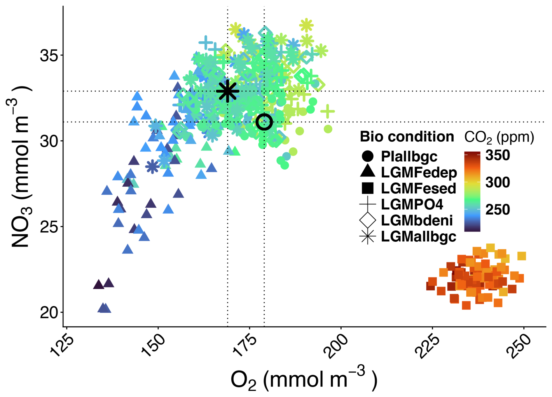
Figure 8 Globally-averaged ${{\mathrm{NO}}_{\mathrm{3}}}^{-}$ vs. O₂ in the 480 simulations. Color represents atmospheric pCO₂ and symbols indicate the different biogeochemical configurations. The black open circle and asterisk indicate mean ${{\mathrm{NO}}_{\mathrm{3}}}^{-}$ and O₂ in PIctl_PIallbgc and LGMatmctl_LGMallbgc simulations, respectively. The cluster of points with high pCO₂ and low ${{\mathrm{NO}}_{\mathrm{3}}}^{-}$ is from *_LGMFesed simulations.

Such a decrease in ${{\mathrm{NO}}_{\mathrm{3}}}^{-}$ as simulated by some of the experiments is in conflict with the observational records. Thus, a low ${{\mathrm{NO}}_{\mathrm{3}}}^{-}$ inventory indicates that a strong decrease in pCO₂ might be due to the wrong reasons in the model, e.g., overestimation of the marine biological carbon pump. On the other hand, the strong Fe limitation in *_LGMFesed simulations results in a decrease in ${{\mathrm{NO}}_{\mathrm{3}}}^{-}$ due to suppressed N₂ fixation, an increase in pCO₂ due to reduced primary production, and higher O₂ concentrations as a result of lower O₂ consumption from POM export (Fig. 8). This increase in O₂ is also inconsistent with proxy-based reconstructions. Those different ${{\mathrm{NO}}_{\mathrm{3}}}^{-}$, O₂, and pCO₂ values highlight the critical role of Fe supply for the LGM model experiments.

4.5 Changes in atmospheric pCO₂ and elemental ratio shifts in POM

In the LGMatmctl_LGMallbgc configuration, the average pCO₂ is 43.5 ppm lower than in PIctl_PIallbgc (Fig. S4x and Table S1). The biogeochemical boundary conditions combined contribute less than the physical boundary conditions. The changes in pCO₂ from *_PIallbgc to *_LGMallbgc (biogeochemical) with PIctl and LGMatmctl configurations are −0.8 and −9.3 ppm, respectively, while the changes from PIctl to LGMatmctl (physical) with *_PIallbgc and *_LGMallbgc conditions are −34.2 and −42.7 ppm, respectively (Table S1). The decreasing pCO₂ due to the LGM physical configuration with *_PIallbgc (−34.2 ppm, PIctl_PIallbgc to LGMatmctl_PIallbgc) agrees with a 33 ppm decrease in a previous model experiment considering changes in physical boundary conditions (Ödalen et al., 2020). Nevertheless, the contribution from the LGM biogeochemical boundary conditions (*_PIallbgc to *_LGMallbgc) to the decrease in pCO₂ is small, and the 43.5 ppm decrease from PIctl_PIallbgc to LGMatmctl_LGMallbgc are only about 50 % of the observed (≈90 ppm; Monnin et al., 2001). The main goal of our experiments is to evaluate changes in some biogeochemical and physical aspects that could affect pCO₂, and not all processes, such as brine-induced stratification (Bouttes et al., 2011) and air-sea disequilibrium (Khatiwala et al., 2019), are considered. These missing processes might also contribute to the ocean receiving less carbon from terrestrial sources than suggested by observational estimates. In our simulations, terrestrial carbon input into the ocean-atmosphere system ranges from 177 ± 1 Pg C in LGMatmctl to 198 ± 1 Pg C in LGMatmpi simulations. These simulated values are slightly lower than the lower bound of the observational estimate of 511 ± 289 Pg C, which is based on δ¹³C measurements from benthic foraminifera (Peterson et al., 2014).

Some earlier experiments using Earth system models were able to generate a larger decline in the pCO₂ (−64 to −84 ppm; Ödalen et al., 2020; Vollmer et al., 2022; Matsumoto et al., 2020a). However, these model experiments only consider the increase in atmospheric Fe deposition but not the decline in the supply from the sediment, which was included in our *_LGMallbgc conditions. When considering only the effects of Fe deposition, the average pCO₂ in the LGMatmctl_LGMFedep simulations is 63 ppm lower than in PIctl_PIallbgc, i.e., 20 ppm more than for LGMatmctl_LGMallbgc. Further, different parameter combinations also affect the changes in pCO₂, e.g., the maximum pCO₂ drawdown in LGMatmctl_LGMFedep is 75 ppm (Fig. S4x), which is close to the observations. It is worthwhile to mention that increased Fe deposition alone reduces atmospheric pCO₂ by 22.7 ppm from PIctl_PIallbgc to PIctl_LGMFedep, which is close to the changes in other model experiments considering only LGM dust deposition under pre-industrial climate conditions (14–22.8 ppm; Nickelsen and Oschlies, 2015; Ödalen et al., 2020; Matsumoto et al., 2020a).

The effects of variable stoichiometry on atmospheric pCO₂ changes during the LGM have been examined in several previous studies. These include an empirical relationship between pC : P and ambient ${{\mathrm{PO}}_{\mathrm{4}}}^{\mathrm{3}-}$, and between pC : N and ambient ${{\mathrm{NO}}_{\mathrm{3}}}^{-}$ (Galbraith and Martiny, 2015), as well as a power law formulation for pC : P and pC : N that considers the influences of ambient ${{\mathrm{PO}}_{\mathrm{4}}}^{\mathrm{3}-}$ and ${{\mathrm{NO}}_{\mathrm{3}}}^{-}$, temperature, and light intensity (Matsumoto et al., 2020a). For models that adopt the empirical relationship between pC : P and ambient ${{\mathrm{PO}}_{\mathrm{4}}}^{\mathrm{3}-}$, the magnitude of the pCO₂ decline increases by 13–16 ppm (Ödalen et al., 2020; Fillman et al., 2023). When the relationship between pC : N and ambient ${{\mathrm{NO}}_{\mathrm{3}}}^{-}$ is also considered, the increase reaches 11 ppm (Matsumoto et al., 2020a). The power-law formulation of Matsumoto et al. (2020a) leads to an additional drawdown of 20 ppm compared to a fixed stoichiometry scheme using the Redfield ratio $\mathrm{C}:\mathrm{N}:\mathrm{P}=\mathrm{106}:\mathrm{16}:\mathrm{1}$.

To facilitate comparison with studies neglecting the changes in sedimentary Fe flux, benthic N-loss, and ${{\mathrm{PO}}_{\mathrm{4}}}^{\mathrm{3}-}$ inventory, we calculate the changes in pC : N (26 %) and pC : P (28 %) from PIctl_PIallbgc to LGMatmctl_LGMFedep, which isolates the effect of enhanced atmospheric Fe deposition in our simulations. Multiplying the relative changes by the total pCO₂ decline yields an estimated additional drawdown of approximately 16–17 ppm attributable to variable stoichiometry.

While this simple calculation neglects spatial variations, it provides a first-order estimate of the impact of stoichiometric flexibility on atmospheric pCO₂ drawdown, showing that the effects of changes in elemental ratios on pCO₂ in our simulations agree with previous studies considering the effects of Fe deposition.

In our experiments, pC : N and pC : P are lower under full LGM conditions (LGMatmctl_LGMallbgc) by 8 % and 10 %, respectively, than in PIctl_PIallbgc. In LGMatmctl_LGMallbgc, the higher surface nutrient concentrations, resulting from the weaker biological utilisation due to a lower global temperature and reduced Fe supply from the sediment, largely influence the elemental ratios of POM, as shown in the *_LGMFesed simulations. Nevertheless, the lower pC : N and pC : P could be simply linked to extra N and P incorporated into the POM, and do not necessarily indicate that the effects of variable stoichiometry of POM on atmospheric pCO₂ are reversed in LGMatmctl_LGMallbgc. We note, however, that regional variations, particularly in regions such as the Southern Ocean, may differ from the global mean response and could play a more important role locally.

4.6 Effects of parameter variations

The ranges of variation in the model’s parameter values, which generally reflect ranges of uncertainty, contribute significantly to the variability of the simulated carbon cycle responses during the Last Glacial Maximum (LGM) and form a central motivation for this study. This variability arises because the response of biogeochemical tracers and fluxes to changes in boundary conditions depends strongly on the choice of the combination of parameter values.

The changes in Fe supply greatly affect the mean changes in the tracers and fluxes when compared with the pre-industrial simulations, and also contribute to higher variability among the 20 simulations with different parameter settings for each model configuration (Figs. S4 and S5). It is not surprising that the variations among the 20 ensemble members are often stronger when the median values deviate more from the pre-industrial simulations, but that is not always the case. For example, ${{\mathrm{NO}}_{\mathrm{3}}}^{-}$ shows a different behaviour. When compared with *_PIallbgc, the deviation of the median is highest in *_LGMFesed but the variation is much larger in *_LGMFedep (Fig. S4c). That is because the ${{\mathrm{NO}}_{\mathrm{3}}}^{-}$ level is affected by N₂ fixation, WC and benthic denitrification, and the shut-down of WC denitrification in *_LGMFesed subdues the variations in ${{\mathrm{NO}}_{\mathrm{3}}}^{-}$.

Compared to the pre-industrial reference condition (PIctl_PIallbgc), atmospheric pCO₂ under full LGM conditions (LGMatmctl_LGMallbgc) decreases by 36 to 58 ppm among the 20 simulations. The difference between the minimum and maximum pCO₂ changes amounts to 50 % of the 43.5 ppm average decrease. We apply the lm (fitting linear model) function in R package “stats” to calculate P values for the correlations between changes in pCO₂ from PIctl_PIallbgc to LGMatmctl_LGMallbgc (ΔpCO₂) and in the perturbed parameters to better understand how individual parameters contribute to the pCO₂ variation (P<0.05, Fig. S10). Among the 19 parameters, the nitrogen subsistence quota ($Q_{\mathrm{0},\text{phy}}^{\text{N}}$), temperature-dependent mortality (λ_0,phy), and zooplankton maximum specific ingestion rate (g_max) are significantly associated with the ΔpCO₂ (Fig. S10b, e, and m). Thus, not only phytoplankton- but also zooplankton (top-down)-related parameters affect the variations in pCO₂ in our simulations.

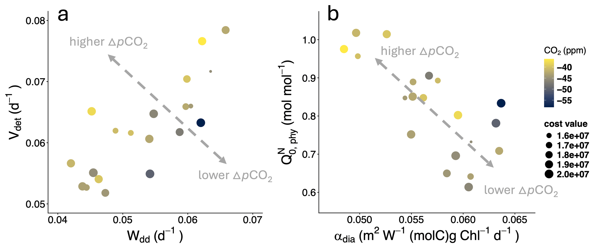
Figure 9 Effects of parameter pairs on the ΔpCO₂ between PIctl_PIallbgc and LGMatmctl_LGMallbgc. (a) ν_det and w_dd and (b) α_dia and $Q_{\mathrm{0},\text{phy}}^{\text{N}}$ are the most positively and negatively correlated pairs in the 19 parameters, respectively.

Overall, the selected 20 parameter sets yield strongly different biogeochemical fluxes, inventories, and atmospheric pCO₂ in our various LGM model configurations. The spread in simulated changes relative to pre-industrial conditions (PIctl, PIallbgc, and PIctl_PIallbgc) across the 20 ensemble members arises from differences in how the selected parameter sets control model sensitivity to LGM boundary conditions in each configuration. Interestingly, the ΔpCO₂ appears unrelated to cost values based on the likelihood-based cost function we employed for the parameter selection (Fig. S10t). Indeed, the ΔpCO₂ is not necessarily correlated with cost values, which may be explained by different correlations (a) among parameters within the best 20 parameter sets, (b) between parameters and cost values, and (c) between parameters and ΔpCO₂. This is easiest to see when the best selection of values of a pair of parameters is highly correlated. It means that collinearities exist, with effects on the cost function that are strongly interconnected. For example, ν_det and w_dd are the strongest positively-correlated pair among the 19 parameters (Fig. S11), and because changes in ν_det and w_dd have opposite effects on ΔpCO₂ (Fig. S10), they tend to compensate each other's effect on ΔpCO₂ in the LGMatmctl_LGMallbgc simulations. Thus, the pairs in the best 20 parameter sets yield limited changes in the ΔpCO₂, and a strong deviation in the ΔpCO₂ can only occur when ν_det and w_dd change in opposite directions (Fig. 9a). The other case would be α_dia and $Q_{\mathrm{0},\text{phy}}^{\text{N}}$, which is the strongest negatively-correlated pair among the 19 parameters (Fig. S11). Since changes in α_dia and $Q_{\mathrm{0},\text{phy}}^{\text{N}}$ also have opposite effects on the ΔpCO₂, opposing changes in α_dia and $Q_{\mathrm{0},\text{phy}}^{\text{N}}$ could result in a larger deviation in the ΔpCO₂ but the effects on the cost values remains limited (Fig. 9b), owing to a weak correlation of either parameter with the cost value among the best 20 simulations. The weak relationship between the ΔpCO₂ and cost values demonstrates the complexity of LGM model simulations with respect to the parameter settings, and emphasises the importance of perturbed parameter ensemble simulations.

5 Conclusion and Future Directions

We investigate the role of several physical and biogeochemical boundary conditions in the face of parameter uncertainty in an Earth system model for simulating marine biogeochemistry and atmospheric pCO₂ under pre-industrial and LGM conditions. We find that persistent changes in Fe supply are the most critical factor, while changes in major nutrients (${{\mathrm{NO}}_{\mathrm{3}}}^{-}$ or ${{\mathrm{PO}}_{\mathrm{4}}}^{\mathrm{3}-}$) alone have limited effects, at least partly due to co-limitation effects and the variable stoichiometry of POM in the model. The results from simulations with different combinations of physical and biogeochemical boundary conditions show that physical boundary conditions also affect marine biogeochemical cycles and atmospheric pCO₂, and the variable pP : C and pN : C can contribute about 16–17 ppm additional drawdown of pCO₂ when considering LGM Fe deposition alone.

Due to the decline in sedimentary Fe input, productivity decreases and leads to higher surface ${{\mathrm{NO}}_{\mathrm{3}}}^{-}$ and ${{\mathrm{PO}}_{\mathrm{4}}}^{\mathrm{3}-}$ in the LGM than the pre-industrial simulations. This mechanism is often ignored in LGM modelling studies. Nevertheless, we show that it could have strong impact on marine biogeochemical cycles, elemental ratios of POM, and the changes in the pCO₂. This Fe source to the ocean thus requires further understanding and examination.

The variation of pCO₂ changes among the 20 LGM simulations highlights the uncertainty when applying parameter sets calibrated using pre-industrial conditions. We argue that understanding the uncertainty introduced by different boundary conditions and parameter sets is critical for accurately simulating LGM pCO₂ dynamics and the interactions between physical and biogeochemical factors in Earth system models.