the Creative Commons Attribution 4.0 License.
the Creative Commons Attribution 4.0 License.
 | 21 Dec 2020
Emergent constraints on equilibrium climate sensitivity in CMIP5: do they hold for CMIP6?
Axel Lauer
Pierre Gentine
Steven C. Sherwood
Veronika Eyring
An important metric for temperature projections is the equilibrium climate sensitivity (ECS), which is defined as the global mean surface air temperature change caused by a doubling of the atmospheric CO2 concentration. The range for ECS assessed by the Intergovernmental Panel on Climate Change (IPCC) Fifth Assessment Report is between 1.5 and 4.5 K and has not decreased over the last decades. Among other methods, emergent constraints are potentially promising approaches to reduce the range of ECS by combining observations and output from Earth System Models (ESMs). In this study, we systematically analyze 11 published emergent constraints on ECS that have mostly been derived from models participating in the Coupled Model Intercomparison Project Phase 5 (CMIP5) project. These emergent constraints are – except for one that is based on temperature variability – all directly or indirectly based on cloud processes, which are the major source of spread in ECS among current models. The focus of the study is on testing if these emergent constraints hold for ESMs participating in the new Phase 6 (CMIP6). Since none of the emergent constraints considered here have been derived using the CMIP6 ensemble, CMIP6 can be used for cross-checking of the emergent constraints on a new model ensemble. The application of the emergent constraints to CMIP6 data shows a decrease in skill and statistical significance of the emergent relationship for nearly all constraints, with this decrease being large in many cases. Consequently, the size of the constrained ECS ranges (66 % confidence intervals) widens by 51 % on average in CMIP6 compared to CMIP5. This is likely because of changes in the representation of cloud processes from CMIP5 to CMIP6, but may in some cases also be due to spurious statistical relationships or a too small number of models in the ensemble that the emergent constraint was originally derived from. The emergently- constrained best estimates of ECS also increased from CMIP5 to CMIP6 by 12 % on average. This can be at least partly explained by the increased number of high-ECS (above 4.5 K) models in CMIP6 without a corresponding change in the constraint predictors, suggesting the emergence of new feedback processes rather than changes in strength of those previously dominant. Our results support previous studies concluding that emergent constraints should be based on an independently verifiable physical mechanism, and that process-based emergent constraints on ECS should rather be thought of as constraints for the process or feedback they are actually targeting.
- Article
(3350 KB) - Full-text XML
- BibTeX
- EndNote


A bulk measure of the sensitivity of the climate system to carbon dioxide in the atmosphere (CO2) is commonly expressed by the equilibrium climate sensitivity (ECS), an idealized metric defined as the mean global surface air temperature change that results from a doubling of the atmospheric CO2 concentration over pre-industrial levels once the climate system reached equilibrium. In 1979, the Charney report determined an ECS range of 1.5 to 4.5 K for the Earth system (Charney et al., 1979). This range had not changed substantially by the time of the Intergovernmental Panel on Climate Change (IPCC) Fifth Assessment Report (AR5) (Collins et al., 2013) and is close to the range of the Earth system models participating in the Coupled Model Intercomparison Project Phase 5 (CMIP5, Taylor et al., 2012).
This large range of model climate sensitivity values can be largely attributed to differences in cloud feedbacks (Boucher et al., 2013). In particular, model differences in the change in shortwave reflection of low-level clouds changes in response to climate change dominate the uncertainties in the global warming projections, particularly in the tropics but also at midlatitudes (Brient and Schneider, 2016; Vial et al., 2013). Over the years, various lines of evidence have been exploited to constrain the range of ECS, including paleoclimate data and analysis of the current observed warming trend (Knutti et al., 2017a). A new assessment using this evidence has narrowed the 66 % range (17 %–83 %) to 2.6–3.9 K (Sherwood et al., 2020), but in the meantime CMIP6 models are displaying a wider range of ECSs (see below).
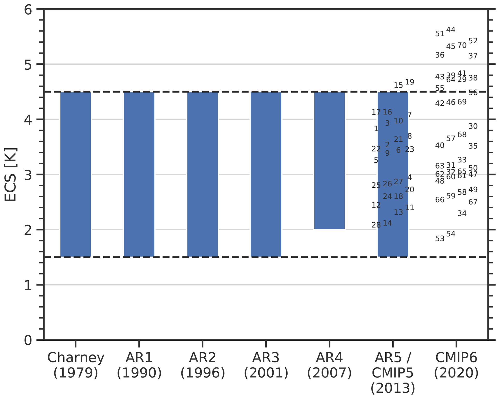
Figure 1Assessed ECS ranges (blue bars) from the Charney report (Charney et al., 1979) and the different Assessment Reports (ARs) of the Intergovernmental Panel on Climate Change (IPCC). The numbers correspond to individual CMIP5 and CMIP6 models; see Tables A1 and A2 for details. Adapted and updated from Meehl et al. (2020).
The use of emergent constraints is another promising approach to reduce the uncertainty in ECS (Eyring et al., 2019). Originally applied to the hydrological cycle and the snow–albedo feedback (Allen and Ingram, 2002; Hall and Qu, 2006), emergent constraints offer the possibility to constrain future projections of Earth system model (ESM) ensembles with observations. Their theoretical basis is an emergent relationship between an observable quantity in the past or present-day climate and a quantity related to the future climate (such as ECS). Typically, the observable quantity is related to a climate feedback, allowing the emergent relationship to be physically motivated by some key processes driving this feedback. Such a physical mechanism is a crucial prerequisite for the plausibility of an emergent constraint: due to large number of possible observables and small number of models, spurious emergent relationships are possible just by chance, which was shown by statistical tests (Caldwell et al., 2014). Caldwell et al. (2018) evaluated the credibility of several published emergent constraints on ECS. Using a feedback decomposition analysis, they assessed whether the published emergent relationship could be explained by the proposed mechanism. Out of 19 emergent constraints on ECS, only 4 of them were considered credible, while the rest of them were either considered not plausible or could not be tested using this approach. In addition, Caldwell et al. (2018) performed out-of-sample tests on five emergent constraints originally trained on older CMIP versions, by applying them to the CMIP5 ensemble. They found that out only one of the five passed this test.
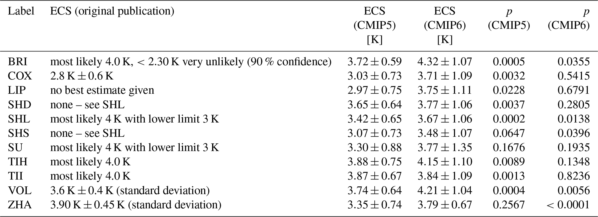
Table 1Overview of the 11 emergent constraints on the ECS used in this study. Observations marked with an asterisk (*) are identical to the ones used in original publication.

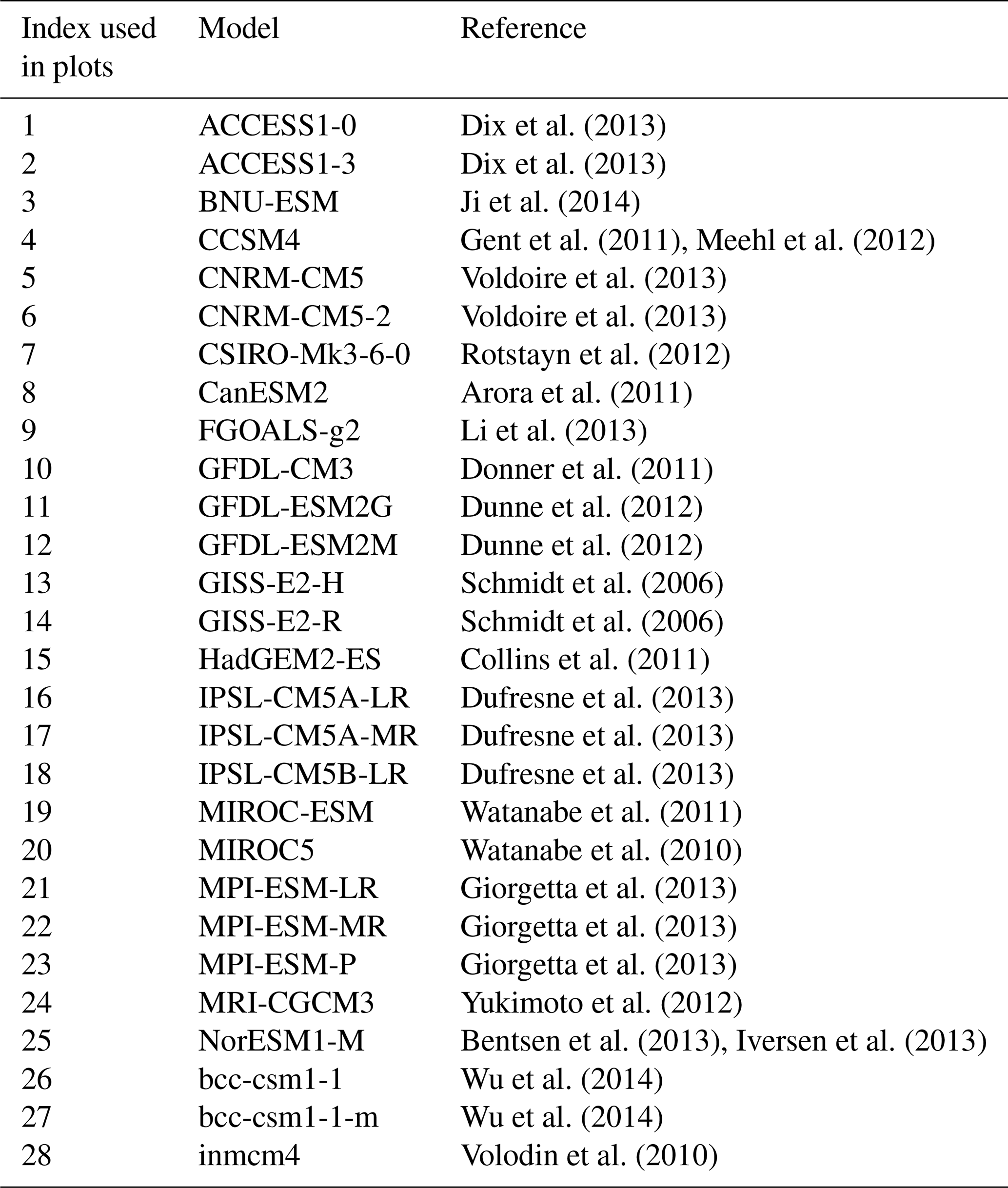
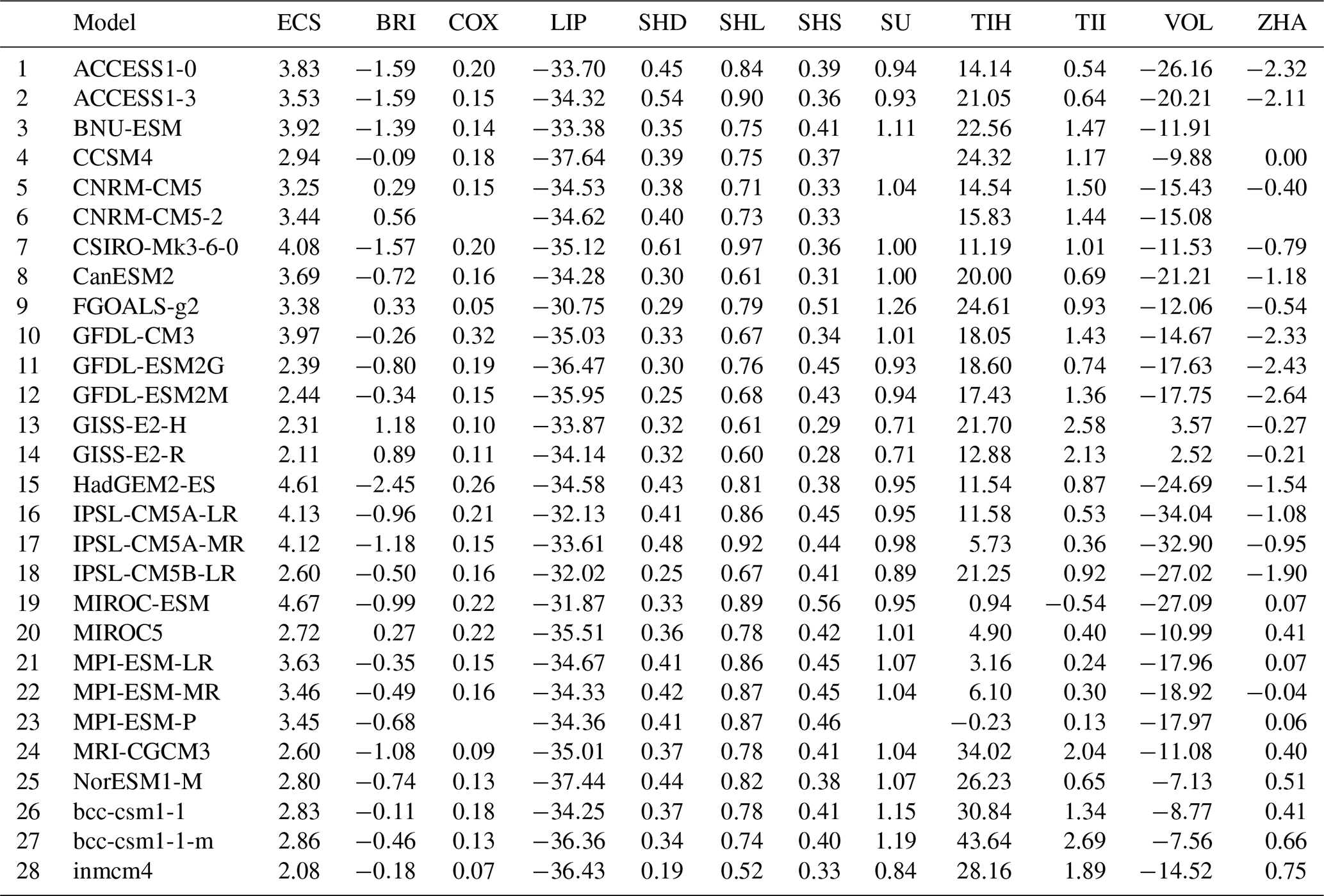
Table 2List of CMIP5 models alongside the index used in the figures of this study and a reference.
In this paper, we follow up on the work of Caldwell et al. (2018) by analyzing 11 published emergent constraints on ECS, which are summarized in Table 1, and assessing whether they still hold for the new CMIP6 model ensemble (Eyring et al., 2016). We first calculate these emergent constraints for the most recent ensemble used to derive all but one of them – CMIP5 (Taylor et al., 2012) – and then test whether they still hold in the CMIP6 ensemble. The one exception is the emergent constraint of Volodin (2008), which was derived on CMIP3 data. While the model range of ECS in CMIP5 is between 2.1 and 4.7 K, the CMIP6 model range is considerably larger, 1.8 to 5.6 K (Meehl et al., 2020); see Fig. 1. Possible reasons for this increased ECS range are changes in the extratropical cloud parameterizations and microphysics in the CMIP6 models (Zelinka et al., 2020). However, despite including more detailed cloud physical processes, further analyses suggest that the high-sensitivity models might overestimate the future warming trend (Tokarska et al., 2020). The large ECS range in CMIP6 emphasizes the need for reliable methods to constrain the uncertainty range of future climate projections with observations. The CMIP6 ensemble can be used for an independent testing of the constraints on previously unknown data. If the proposed underlying physical mechanisms are robust, i.e., targeting a key feedback mechanism controlling most of the observed CMIP6 spread, the emergent constraints would be expected to hold when applied to CMIP6 data. In this analysis we thus test the robustness of the constraints to new models and models with advances in model design over time.
Section 2 provides an overview of the data and methods used. Section 3 gives a discussion of the 11 emergent constraints on ECS and their results when derived from the CMIP5 or CMIP6 ensemble, including an analysis of their statistical significance. The paper ends with a discussion and summary in Sects. 4 and 5.
2.1 Equilibrium climate sensitivity (ECS)
In this study we use the output from climate models participating in CMIP5 and CMIP6, shown in Tables 2 and 3, respectively. Traditionally, ECS is defined as the global mean surface air temperature change after an instantaneous doubling of the atmospheric CO2 concentration once the climate system reaches radiative equilibrium. Since running a fully coupled ESM into equilibrium is computationally expensive (this would require thousands of model years; see Rugenstein et al., 2020), ECS is typically approximated by a so-called “effective climate sensitivity”, which is derived from the first 150 years that follow an instantaneous quadrupling of the atmospheric CO2 concentration (4×CO2 run). Since the ESMs are not in radiative equilibrium during these 150 years, a regression of the top-of-atmosphere net downward radiation N versus the global mean surface air temperature change ΔT extrapolated to N=0 gives an estimate of the equilibrium warming (Gregory et al., 2004). In this paper, we use the term “ECS” to denote this effective climate sensitivity derived from the Gregory regression method. In this calculation, the linear fit of a corresponding pre-industrial control run is subtracted from the 4×CO2 run to account for energy leakage and remove any model drift that is present in the control climate without adding noise (Andrews et al., 2012).
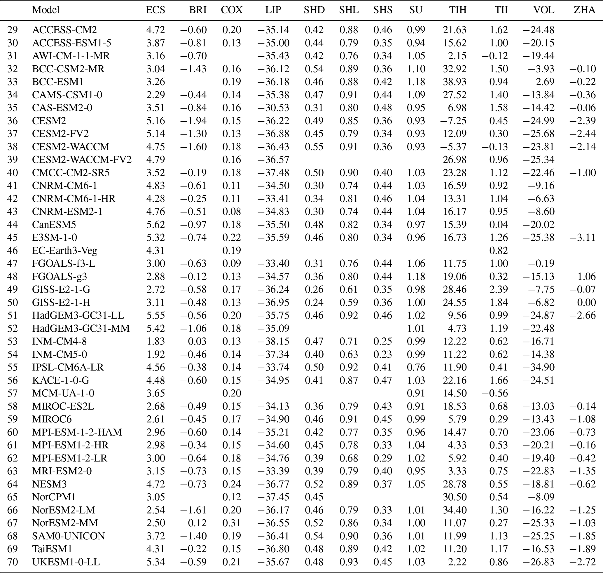
Table 3As in Table 2 but for CMIP6 models included in this study.

Even though it is widely used in literature, this Gregory regression method is known to be only an approximation of the true climate sensitivity. As shown by Sherwood et al. (2020), the effective climate sensitivity is 6 % lower than the best estimate of the true equilibrium warming obtained from integrating the climate models until a new equilibrium is reached. This number is a model-based estimate of the compensation between changing feedbacks with time and the differences introduced by considering a 4×CO2 run instead of a 2×CO2 run. However, only a few ESMs provide simulations long enough to assess the true climate sensitivity. The CMIP endorsed LongRunMIP (Rugenstein et al., 2019) could be a promising way to estimate the true climate sensitivity that can then be used to reevaluate emergent constraints and their proposed underlying physical mechanisms.
2.2 Calculation of emergent constraints on ECS
An overview of the 11 emergent constraints analyzed in this study including the variables required for their calculations is given in Table 1 and the following section. We chose these particular emergent constraints since these were already implemented in the ESMValTool (see Sect. 2.4) at the time of writing this study, which greatly facilitated this analysis. For all emergent constraints, we use the historical simulations of CMIP5 and CMIP6 in order to ensure maximum agreement with the observational data. If necessary, the historical simulation of CMIP5 is extended after its final year 2005 with data from the RCP8.5 scenario (Riahi et al., 2011). Note that we only use data through 2014, during which time all RCP scenarios behave similarly and the choice of the scenario is not expected to affect results considerably. Such an extension is not needed for CMIP6 models as their historical simulations cover a longer time period until 2014.
To evaluate the resulting constrained probability distribution of ECS, we use the following nomenclature: let xm be the x axis variable (i.e., the observable, constraining variable) of climate model m and ym its corresponding target variable (ECS in our case). Following Cox et al. (2018), we use ordinary least-squares regression to fit the linear model
where is the predicted target variable for predictor xm, a the intercept of the linear regression line and b the slope of the linear regression line. Fitting the regression model includes minimizing the standard error of the estimate
where M is the total number of climate models.
In the standard emergent constraint approach, the constrained target variable y (here ECS) is given by the regression evaluated at an observed or observationally based (in case of using reanalysis data) value x that has not been used to fit the regression line. In that case, the corresponding uncertainty in the prediction of is given by the standard prediction error
Here, is the arithmetic mean of x over all models. Assuming Gaussian errors, this equation defines the conditional probability density function (PDF) for predicting a value of y given x, i.e., the posterior distribution:
This distribution can be interpreted as the posterior distribution in the regression model based on climate model output but constrained by matching the observable x. However, the observation of x (referred to as x0) is not error free and has uncertainties associated with it. Assuming again an unbiased Gaussian, the resulting observational probability density for observing x0 given the true value x is given by
where is the variance of the observation about the true value. Assuming a uniform prior P(x)∝1 with no cut-offs (i.e., the cut-offs are positive and negative infinity, which forms an “improper” prior) and using Bayes' theorem implies P(x|x0)=P(x0|x). In a final step, numerical integration is used to calculate the marginal probability density for the constrained prediction of the target variable y dependent on the observation x0:
By assuming a uniform prior in x, we also assume a uniform prior in y (the true ECS), since x and y are linearly related (see Eq. 1); in other words, an ECS near 8 K would be deemed just as probable as one near 4 K if both are equally consistent with the observational best estimate x0. We do this for simplicity. The PDFs would shift somewhat lower with a broad prior on processes instead (see Sherwood et al., 2020), but we are concerned here with how outcomes compare using CMIP5 versus CMIP6 data, rather than the exact ranges obtained. Such comparisons are not sensitive to the prior.
As typically done in other studies proposing a single emergent constraint on ECS, we do not explicitly take model interdependency into account when applying the linear regression model (see Eq. 1) to the model ensemble data. We simply assume that the individual data points (i.e., climate models) are independent. As some modeling groups provide output from multiple ESMs and some ESMs from different modeling groups share components and code, this is clearly not the case. Duplicated code in multiple models is expected to lead to an overestimation of the sample size of a model ensemble and may result in spurious correlations (Sanderson et al., 2015). Possible approaches could be to stop treating all models equally by either applying a model weighting based on a model's interdependence with the other models or by simply reducing the ensemble size considering models only that are above a given (yet to be defined) interdependence score. Promising approaches to quantify the model interdependency that could be followed include, for example, the studies of Sanderson et al. (2015, 2017) and Knutti et al. (2017b).
Another limitation of our approach is the statistical model itself. Similar to many other emergent constraint studies, we use an ordinary least-squares linear regression model for each emergent constraint. However, in some cases this might not be appropriate, e.g., when we expect nonlinear behavior or when physical constraints can be used to derive further constraints for the regression model like a zero intercept (Annan et al., 2020; Jimenez-de-la-Cuesta and Mauritsen, 2019; Renoult et al., 2020).
We further note that observational uncertainties can also play a role, as using different observational datasets for a given variable as a proxy for observational uncertainty might lead to different emergent constraints. As this study uses only one combination of observational datasets to calculate the emergent constraints, as was the case in the original published emergent constraint studies, the error estimations given by our analysis are expected to underestimate the true error. This could be investigated by systematic tests using different observational datasets and/or combinations thereof as a proxy for observational uncertainty. Where available, additional observational uncertainty estimates could be used to give better estimates of the constrained range of ECS. A major challenge associated with this is, however, to determine how observational uncertainties propagate to the spatial scales and timescales represented by the models because of the not typically well-known correlation of observational errors in space and time (e.g., Bellprat et al., 2017).
2.3 Statistical significance of emergent relationships
To evaluate the statistical significance of the different emergent relationships, we use a two-sided t test to determine how likely the correlation found between the predictors and ECS would be to appear by chance. The null hypothesis for this test is that the predictor and ECS are not linearly correlated, i.e., the true underlying Pearson correlation coefficient of the population is zero. In that case, the variable
has a Student's t distribution with M−2 degrees of freedom; r is the Pearson correlation coefficient evaluated on the sample (xm, ym). In this study, we indicate the statistical significance with the p value, which describes the probability of obtaining an absolute sample Pearson correlation coefficient greater than |r| if the null hypothesis is true, i.e., the predictor and ECS are not linearly correlated. Smaller p values indicate higher significance. Although threshold values such as p<0.05 are often used to declare “significance,” here we focus mainly on how p values are affected by the change from CMIP5 to CMIP6, noting that they may be biased low anyway by the assumptions discussed in Sect. 2.2.
2.4 ESMValTool
All figures in this paper are produced with the Earth System Model Evaluation Tool (ESMValTool) version 2 (Eyring et al., 2020; Lauer et al., 2020; Righi et al., 2020). The ESMValTool is an open-source community diagnostics and performance metrics tool for the evaluation of Earth system models (https://www.esmvaltool.org/, last access: 18 December 2020). An ESMValTool recipe (configuration file defining input data, preprocessing steps and diagnostics to be applied) is available that can be used to reproduce all figures in this paper. This also allows redoing the analysis presented in this study once new model simulations from CMIP6 or other model ensembles become available.
In this section we describe and discuss the 11 emergent constraints on ECS summarized in Table 1 using CMIP5 and CMIP6 data (Sect. 3.1 to 3.11) and provide a best estimate for ECS and statistical significance of the 11 emergent constraints in Sect. 3.12. While most of these emergent constraints have been derived using data from the CMIP5 and/or CMIP3 ensembles, to our knowledge none of them has been evaluated on the CMIP6 ensemble so far. The results for the individual emergent constraints described in the following are shown in Figs. 2 to 5. The left columns in these figures show the emergent relationships, including the uncertainty of the linear regressions (blue and orange shaded areas; see Eq. 3) and the uncertainty in the observations (gray shaded area; see Eq. 5). The right columns show the probability distributions of ECS in the original model ensemble (histogram) and the constrained distribution given by the emergent constraints (blue and orange line; see Eq., 6). Table 4 shows the corresponding 66 % confidence intervals (i.e., 17 %–83 % intervals) of ECS derived from the probability distributions given by Eq. (6) and the p values used to assess the significance of the emergent relationships.
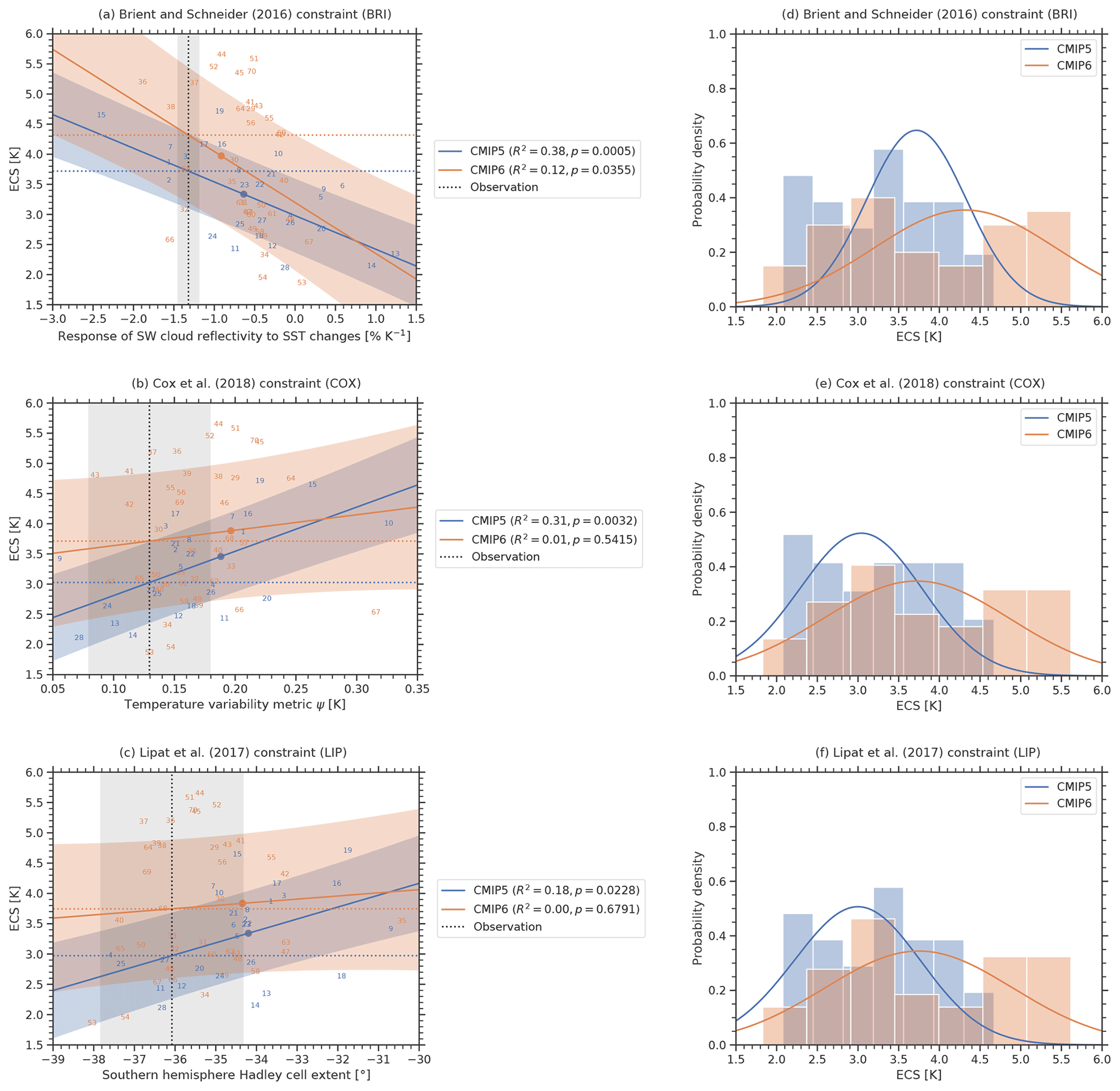
Figure 2Emergent constraints BRI, COX, and LIP applied to the CMIP5 ensemble (blue) and CMIP6 ensemble (orange). (a–c) Emergent relationships (solid blue and orange lines) for the CMIP models (numbers for individual models are specified in Tables A1 and A2). The shaded areas around the regression lines correspond to the standard prediction errors (Eq. 3), which defines the error in the regression model itself. The vertical dashed black line corresponds to the observational reference (see Table 1 for details on the individual observational datasets used) with its uncertainty range given as standard error (gray shaded area). The horizontal dashed lines show the best estimates of the constrained ECS for CMIP5 (blue) and CMIP6 (orange). The colored dots mark the CMIP5 (blue) and CMIP6 (orange) multi-model means. The p value in the legend corresponds to the hypothesis test introduced in Sect. 2.3 and describes the probability to obtain an absolute correlation coefficient |r| or higher under the null hypothesis that the true underlying correlation coefficient between the predictor and ECS is zero. (d–f) Probability densities for the constrained ECS following Eq. (6) (solid lines) and the unconstrained model ensembles (histograms). Note that for each individual emergent constraint, a different subset of climate models is used due to the availability of data (see Tables A1 and A2 for details). Thus, these histograms may differ for the different constraints.
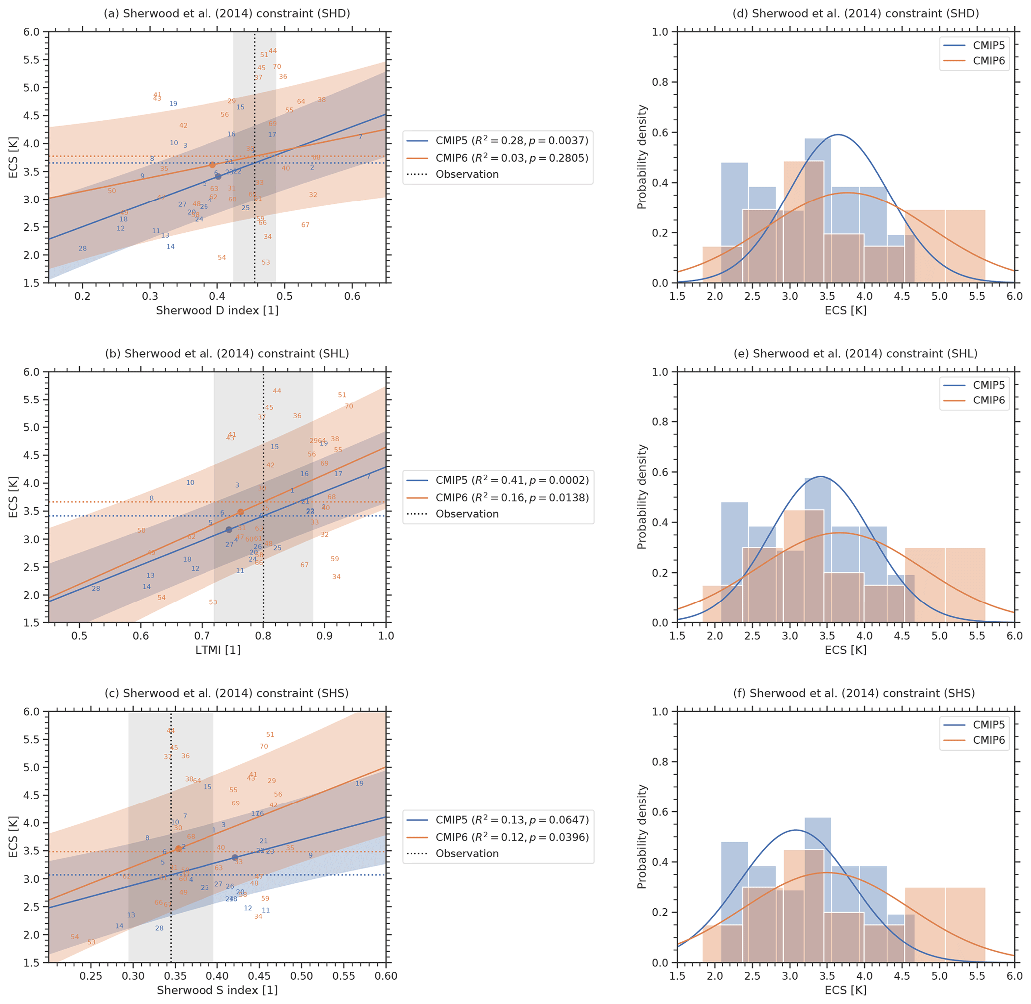
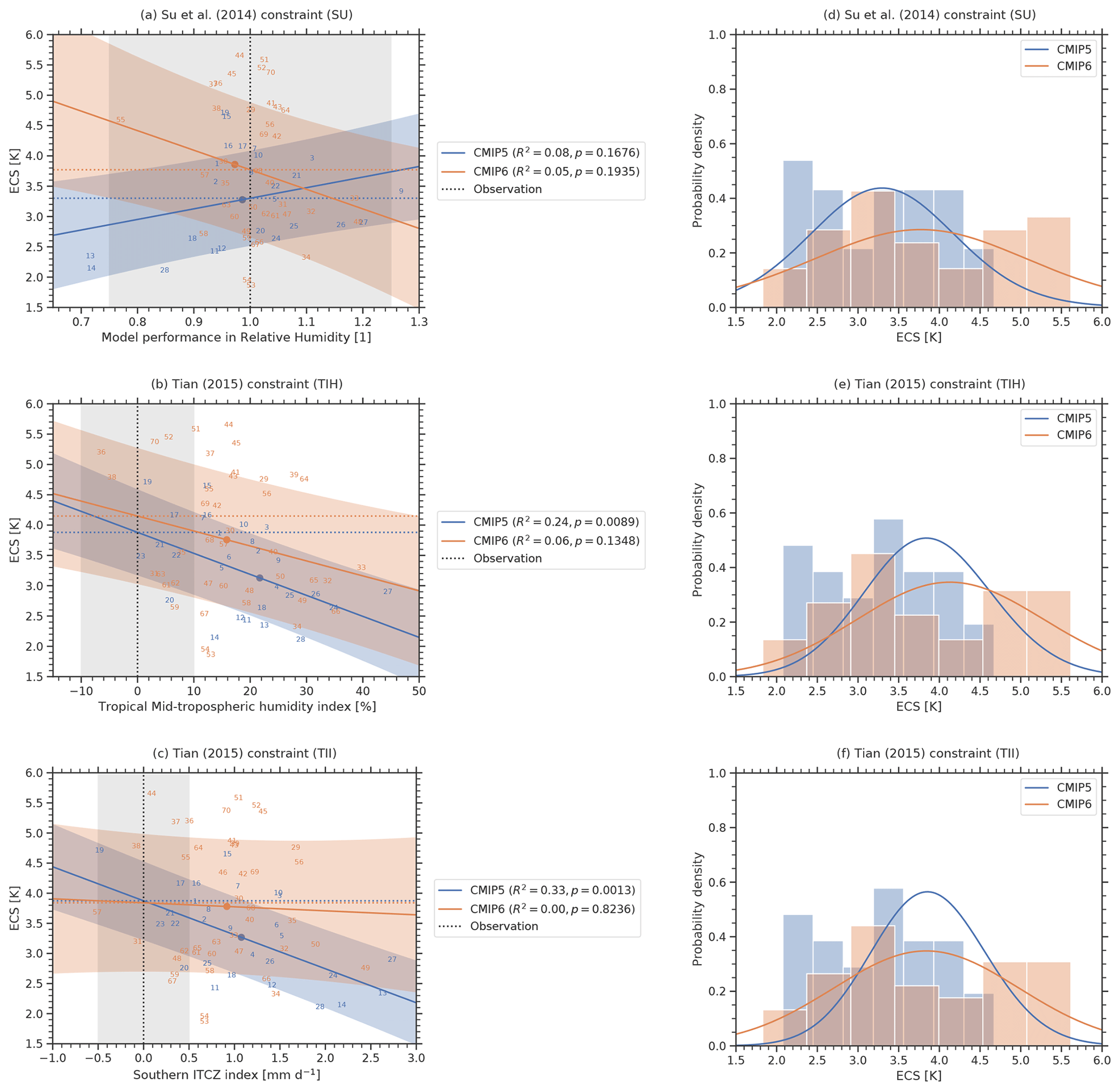
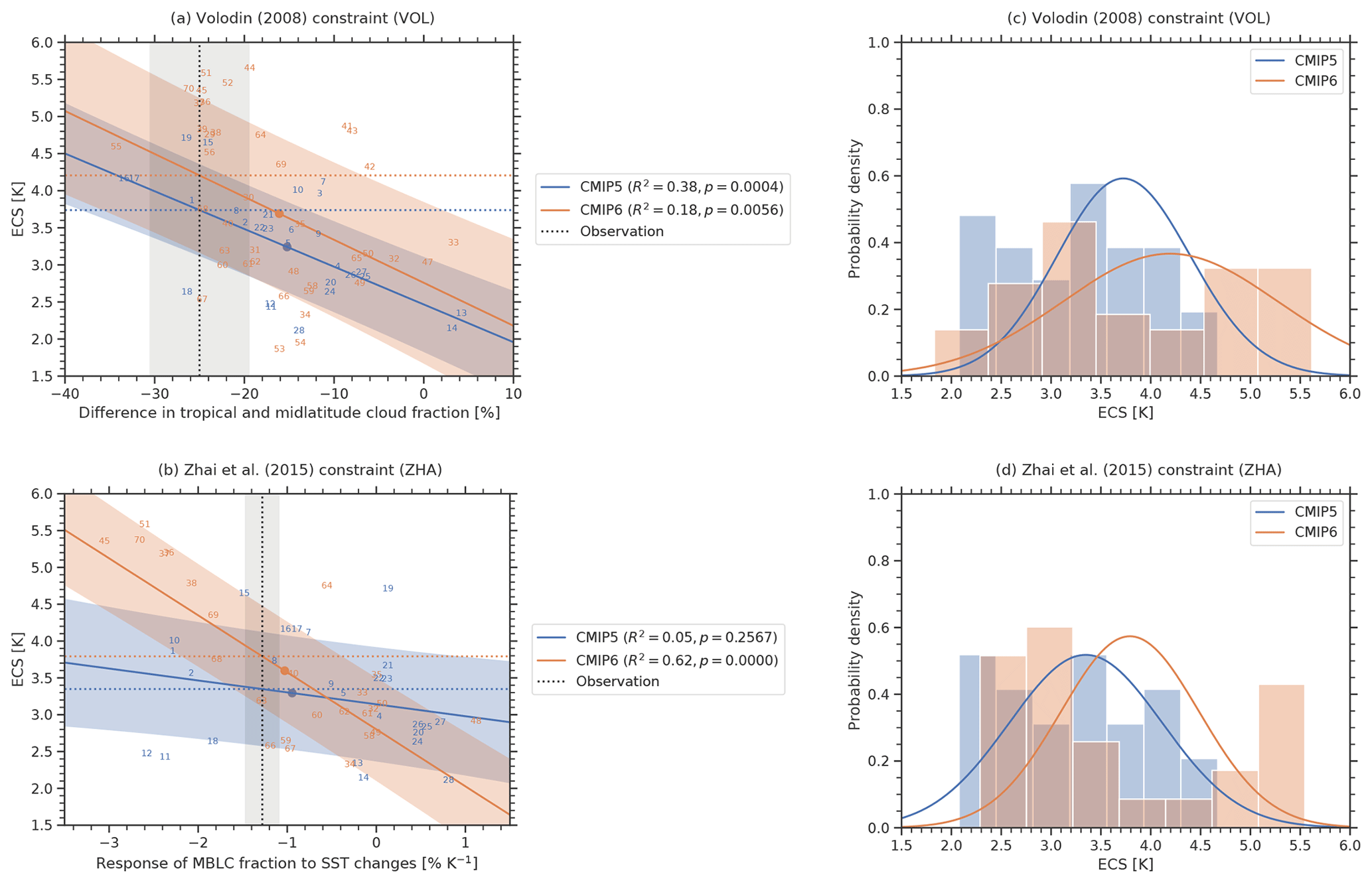
Table 4Overview of the constrained ECS ranges and p values for all 11 analyzed emergent constraints. If not further specified, the uncertainty ranges correspond to the 66 % confidence intervals (17 %–83 %). For CMIP5 and CMIP6, these are evaluated from the probability distribution given by Eq. (6) (see also the right columns of Figs. 2 to 5). Note that even though CMIP5 models were used for some constraints in the original publications, the constrained ranges in column 2 and column 3 might differ due to the use of different models (in this paper, we use output from all CMIP models that is publicly available; see the data availability section for details). The p values describing the significance of the emergent relationships are defined as the probability to obtain an absolute correlation coefficient |r| or higher under the null hypothesis that the true underlying correlation coefficient between the predictor and ECS is zero. Smaller p values point to higher significance and vice versa (for details see Sect. 2.3).
3.1 Response of shortwave cloud reflectivity to changes in sea surface temperature (BRI)
In this emergent constraint proposed by Brient and Schneider (2016), ECS is correlated with the tropical low-level cloud (TLC) albedo, i.e., using the covariance of clouds with changes in sea surface temperatures (SSTs). Differences in the TLC albedo account for more than half of the variance of the ECS in the CMIP5 ensemble. Following Brient and Schneider (2016), TLC regions are defined as grid points that are in the driest quartile of 500 hPa relative humidity of all grid cells over the ocean between 30∘ S and 30∘ N. The albedo of the TLC is obtained by calculating the ratio of TOA shortwave cloud radiative forcing and solar insolation averaged over the TLC region. The regression coefficients of deseasonalized variations of TLC shortwave albedo and SST (in % K−1) are then used as an emergent constraint for ECS. Here, we use observational data from HadISST for SST (Rayner et al., 2003), ERA-Interim for 500 hPa relative humidity (Dee et al., 2011) and CERES-EBAF (Loeb et al., 2018) for the TOA radiative fluxes over the time period 2001–2005. In the original publication, Brient and Schneider (2016) use similar observation-based datasets with the exception of SST, where they take data from the Extended Reconstructed Sea Surface Temperature (Smith and Reynolds, 2003) as reference instead. Our analysis yields a 66 % confidence range for ECS of 3.72 K ± 0.59 K for CMIP5 (R2=0.38) and 4.32 K ± 1.07 K for CMIP6, with much lower R2=0.12. The original publication stated a best estimate of 4.0 K, with a very low likelihood of values below 2.3 K (90 % confidence). The statistical significance of the emergent relationship dropped from p=0.0005 for CMIP5 to p=0.0355 for CMIP6.
3.2 Temperature variability (COX)
The emergent constraint on ECS proposed by Cox et al. (2018) uses a temperature variability metric Ψ that is based on the interannual variation of global mean temperature calculated from its variance (in time) and 1 year lag autocorrelation. In contrast to the majority of emergent constraints that focus on cloud-related processes, this constraint is based on the fluctuation–dissipation theorem, which relates the long-term response of the climate system to an external forcing (ECS) and short-term variations of the climate system (climate variability). This arguably places the constraint on a more solid theoretical foundation, although several questions were raised on the robustness of the results to choices made in the analysis (Brown et al., 2018; Po-Chedley et al., 2018; Rypdal et al., 2018). For example, Annan et al. (2020) showed that the assumed linear relationship between Ψ and ECS does not hold when adding a deep ocean to the model. As observational data, here we use the HadCRUT4 dataset (Morice et al., 2012) over the time period 1880–2014. Under the COX constraint we thus assess a 66 % ECS range of 3.03 K ± 0.73 K for CMIP5 (R2=0.31) and 3.71 K ± 1.09 K for CMIP6 (R2=0.01). Cox et al. (2018) derived a 66 % range of 2.8 K ± 0.6 K from a different subset of CMIP5 models but the same observations. When moving from CMIP5 to CMIP6, the significance of the emergent relation drops massively from p=0.0032 to p=0.5415, respectively.
3.3 Southern Hemisphere Hadley cell extent (LIP)
The results of Lipat et al. (2017) show that the multi-year average extent of the Hadley cell correlates with ECS in CMIP5 models. The Hadley cell edge is defined as the latitude of the first two grid cells from the Equator going south where the zonal average 500 hPa mass stream function calculated from December–January–February means of the meridional wind field changes sign from negative to positive. Lipat et al. (2017) explain this correlation by tying it to the observed correlation of the interannual variability in midlatitude clouds and their radiative effects with the poleward extent of the Hadley cell. For the calculation of the emergent constraint, we use reanalysis data from ERA-Interim (Dee et al., 2011) for the meridional wind speed over the time period 1980–2005. Our application of this emergent constraint gives ECS 66 % ranges of 2.97 K ± 0.75 K for CMIP5 (R2=0.18) and 3.75 K ± 1.11 K for CMIP6 (R2<0.01). The original publication does not specify an ECS range. For CMIP6, the emergent constraint shows a much lower statistical significance (p=0.6791) than for CMIP5 (p=0.0228).
3.4 Large-scale lower-tropospheric mixing (SHD)
Sherwood et al. (2014) proposed that the degree of mixing in the lower troposphere determines the response of boundary-layer clouds and humidity to climate warming, as the associated moisture transport would increase rapidly in a warmer atmosphere due to the Clausius–Clapeyron relationship. The large-scale component D of this mixing is defined as the ratio of shallow to deep overturning. D is calculated from the vertical velocities averaged over two height regions: 850 and 700 hPa for shallow overturning and 600, 500, and 400 hPa for deep overturning. Both quantities are averaged over parts of the tropical ocean region away from the regions of highest SST and strongest mid-level ascent, specifically the region 30∘ S–30∘ N, 160∘ W–30∘ E, wherever air is ascending at low levels. As observationally based data, we use vertical velocities from ERA-Interim (Dee et al., 2011) over the time period 1989–1998 similar to the original publication. We derive ECS 66 % confidence ranges of 3.65 K ± 0.64 K for CMIP5 (R2=0.28) and 3.77 K ± 1.06 K for CMIP6 (R2=0.03). Sherwood et al. (2014) do not give a best estimate for ECS based on the large-scale component of mixing D or its small-scale counterpart S (Sect. 3.5) but instead for the sum of D+S only (see Sect. 3.6). The regression shows a much lower significance for CMIP6 (p=0.2805) than for CMIP5 (p=0.0037).
3.5 Small-scale lower-tropospheric mixing (SHS)
The small-scale mixing S (Sherwood et al., 2014) is calculated from the differences in relative humidity and temperature between 700 and 850 hPa. The differences are averaged over all grid cells within the upper quartile of the annual mean 500 hPa ascent rate (within ascending regions) in the tropics. The tropics are defined as region between 30∘ S and 30∘ N. In the Cloud Feedback Model Intercomparison Project models (CFMIP, Webb et al., 2017), for which convective tendencies were available, upward moisture transport by parameterized convection was shown to increase more rapidly with warming for higher values of S. We use reanalysis data from ERA-Interim (Dee et al., 2011) for temperature and relative humidity to calculate the observationally based constraint (1989–1998). Our analysis shows a 66 % range of ECS of 3.07 K ± 0.73 K for CMIP5 (R2=0.13) and 3.48 K ± 1.07 K for CMIP6 (R2=0.12). The correlation of S and ECS shows a slightly higher significance in the CMIP6 ensemble (p=0.0396) than in the CMIP5 ensemble (p=0.0647). The SHS constraint is one of the two analyzed emergent constraints (ZHA being the other exception) that shows a higher statistical significance for the CMIP6 than for the CMIP5 ensemble.
3.6 Lower tropospheric mixing index (SHL)
The lower tropospheric mixing index (LTMI) formulated by Sherwood et al. (2014) is defined as the sum of the small-scale mixing S (see Sect. 3.5) and the large-scale mixing D (see Sect. 3.4), which are supposed to capture complementary components of the total mixing phenomenon. Sherwood et al. (2014) argue that the increase in dehydration depends on initial mixing linking it to cloud feedbacks and thus also to ECS. For this constraint, we derive an ECS 66 % confidence range of 3.42 K ± 0.65 K for CMIP5 (R2=0.41) and 3.67 K ± 1.06 K for CMIP6 (R2=0.16). Sherwood et al. (2014) give a best estimate of about 4 K with a lower limit of 3 K. Similar to both other constraints by Sherwood et al. (2014), SHD and SHS, the statistical significance of the SHL emergent relation decreased in CMIP6 (p=0.0138) compared to CMIP5 (p=0.0002).
3.7 Error in vertical profile of relative humidity (SU)
Another emergent constraint on ECS that targets uncertainties in cloud feedbacks was proposed by Su et al. (2014). They show that changes in the Hadley circulation are physically connected to changes in tropical clouds and thus ECS. Consequently, the inter-model spread in the change of the Hadley circulation in an ensemble of climate models is well correlated with the corresponding changes in the TOA cloud radiative effect. Moreover, Su et al. (2014) found a correlation between a model's ECS and its ability to represent the present-day Hadley circulation. The latter is calculated from the tropical (45∘ S–40∘ N) zonal-mean vertical profiles of relative humidity from the surface to 100 hPa. These profiles are then used to define the x axis of the SU constraint by calculating a performance metric based on the slope of the linear regression between a climate model's relative humidity profile and the corresponding observational reference. Similarly to the original publication, we use humidity observations from AIRS (Aumann et al., 2003) for pressure levels greater than 300 hPa and MLS-Aura data (Beer, 2006) for pressure levels of less than 300 hPa. Our analysis yields a constrained 66 % range of ECS of 3.30 K ± 0.88 K for CMIP5 (R2=0.08) and 3.77 K ± 1.35 K for CMIP6 (R2=0.05). The original publication gives a best estimate of 4 K with a lower limit of 3 K. Figure 4 shows that in addition to the low R2 values, the emergent relationship shows different slopes for CMIP5 and CMIP6. For the CMIP5, the expected positive correlation is found, while for CMIP6, a negative correlation is found. This suggests that the constraint is not working (any more) when applied to the CMIP6 data. Consequently, the SU constraint shows a weaker statistical significance in the CMIP6 ensemble (p=0.1935) than for the CMIP5 ensemble (p=0.1676). The SU constraint is related to an emergent constraint on ECS proposed by Fasullo and Trenberth (2012), who correlated May–August zonal-mean relative humidity against ECS. In contrast to Su et al. (2014), they did not use the entire tropics, but identified two distinct regions with largest correlation.
3.8 Tropical mid-tropospheric humidity asymmetry index (TIH)
Tian (2015) found a link between mid-tropospheric humidity over the tropical Pacific and simulated moisture, precipitation, clouds, large-scale circulation, and thus ECS in CMIP3 and CMIP5 models. The study explains this link with the similarity of mid-tropospheric humidity and precipitation patterns as both are related to the ITCZ. The proposed tropical mid-tropospheric humidity asymmetry index to constrain ECS is defined as relative bias (in %) in simulated annual mean 500 hPa specific humidity averaged over the Southern Hemisphere (SH) tropical Pacific (30∘ S–0∘ N, 120∘ E–80∘ W) minus the bias averaged over the Northern Hemisphere (NH) tropical Pacific (20∘–0∘ N, 120∘ E–80∘ W) when compared with observations. Similar to the SU constraint, the index proposed by Tian (2015) seems to be related to the emergent constraint by Fasullo and Trenberth (2012), who found correlations between relative humidity of the middle and upper troposphere and ECS. Here, we use humidity observations from AIRS (Aumann et al., 2003) over the time period 2003–2005 as the reference dataset. We assess a 66 % ECS range of 3.88 K ± 0.75 K for CMIP5 (R2=0.24) and 4.15 K ± 1.10 K for CMIP6 (R2=0.06). Tian (2015) specifies a best estimate of 4.0 K. The significance of the emergent relationship dropped massively from p=0.0089 in CMIP5 to p=0.1348 in CMIP6.
3.9 Southern ITCZ index (TII)
In addition to the humidity index, Tian (2015) proposed an emergent constraint on ECS based on the southern ITCZ index (Bellucci et al., 2010; Hirota et al., 2011). This index is defined as the climatological annual mean precipitation bias averaged over the southeastern Pacific (30∘ S–0∘ N, 150–100∘ W). The southern ITCZ index is calculated in mm d−1 and dominated by the so-called double ITCZ, a common problem in many CMIP5 climate models. Tian (2015) found a link between double-ITCZ bias and simulated moisture, precipitation, clouds, and large-scale circulation in CMIP3 and CMIP5 models. He argues that this could explain the link found between the double-ITCZ bias and ECS. As reference data, we use observed precipitation data for the years 1986–2005 from GPCP (Adler et al., 2003). We calculate an ECS 66 % confidence range of 3.87 K ± 0.67 K for CMIP5 (R2=0.33) and 3.84 K ± 1.09 K for CMIP6 (R2<0.01). Tian (2015) specifies a best estimate of 4.0 K. The emergent relationship shows a much lower statistical significance in CMIP6 (p=0.8236) than in CMIP5 (p=0.0013).
3.10 Difference between tropical and midlatitude cloud fraction (VOL)
The study by Volodin (2008) aims at constraining ECS based on the geographical distribution of clouds in climate models. Since this early emergent constraint was originally trained on CMIP3 models, both CMIP5 and CMIP6 are out-of-sample tests for it. Volodin (2008) shows that high ECS models tend to simulate a higher total cloud cover over the southern midlatitudes and a lower total cloud cover over the tropics (relative to the multi-model mean). This can be used to establish an emergent relationship between the ECS and the difference in tropical total cloud cover (28∘ S–28∘ N) and the southern midlatitude total cloud cover (56–36∘ S). Analogous to the original study, we use the ISCCP-D2 data (Rossow and Schiffer, 1991) as observational reference. For the VOL constraint, we calculate a constrained 66 % range of ECS of 3.74 K ± 0.64 K for CMIP5 (R2=0.38) and 4.21 K ± 1.04 K for CMIP6 (R2=0.18), whereas the original publication gives a range of 3.6 K ± 0.4 K (standard deviation) for a climate model ensemble of CMIP3 models. The emergent constraint by Volodin (2008) shows a lower significance in the CMIP6 ensemble (p=0.0056) than in the CMIP5 ensemble (p=0.0004).
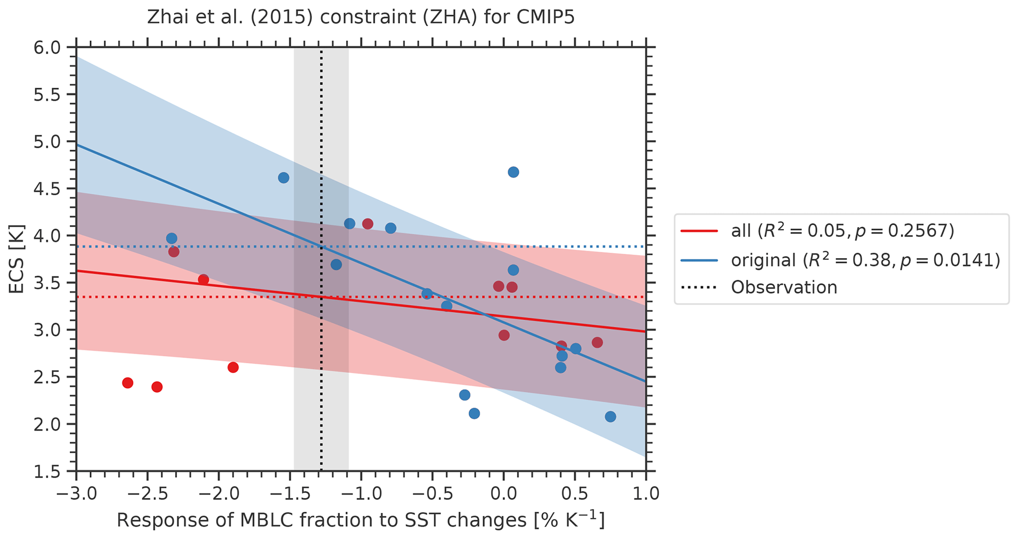
Figure 6Emergent relationship ZHA (Zhai et al., 2015) for different subsets of CMIP5 models. Blue circles show the 15 CMIP5 models used in the original publication (except for CESM1-CAM5): the solid blue line and blue shaded area show the emergent relationships evaluated on these models including the uncertainty range. In our study, we added 11 more CMIP5 models (red circles). The corresponding emergent relationship that considers all available CMIP5 models is shown in red colors. This relationship shows a considerably lower coefficient of determination (R2) and higher p value than the relationship using the original subset of CMIP5 models. The vertical dashed line and shaded area correspond to the observational reference, and the horizontal dashed lines show the corresponding ECS constraints using this observation.
3.11 Response of seasonal marine boundary layer cloud fraction to SST changes (ZHA)
Zhai et al. (2015) focus on the variations of marine boundary layer clouds (MBLCs), which largely contribute to the shortwave cloud feedback and thus to the uncertainty in modeled ECS. Their central quantity is the response of the MBLC fraction to changes in the sea surface temperature (SST) in subtropical oceanic subsidence regions for both hemispheres (20–40∘). On short (seasonal) and long (centennial under a forcing) timescales, this quantity is well correlated with ECS among an ensemble of CMIP3 and CMIP5 models. Together with observations of cloud fraction from CloudSat/CALIPSO (Mace et al., 2009), SST from AMSRE SST (AMSR-E, 2011), and vertical velocity from ERA-Interim (Dee et al., 2011), the seasonal response of MBLC fraction to changes in SST forms an emergent constraint on ECS. We assess a 66 % ECS range of 3.35 K ± 0.74 K for CMIP5 (R2=0.05) and 3.79 K ± 0.67 K for CMIP6 (R2=0.62). In their original publication, Zhai et al. (2015) found an ECS range of 3.90 K ± 0.45 K (standard deviation) for a combination of CMIP3 and CMIP5 models. In terms of statistical significance, the results of the ZHA constraints are somewhat surprising: although CMIP5 data (in combination with CMIP3 data) were successfully used in their original publication, our approach finds that the statistical significance of the emergent relationship is much higher in the unseen CMIP6 ensemble (p<0.0001) than in the previously available CMIP5 ensemble (p=0.2567). The ZHA constraint is the only emergent constraint analyzed here that shows this extreme behavior (only one other constraint, SHS, shows a slightly higher significance in CMIP6; all other constraints show lower significances in CMIP6). The reason for the erratic skill in CMIP5 is the set of climate models used. For our analysis, we use 11 additional CMIP5 models that were not used in the original publication (i.e., ACCESS1-0, ACCESS1-3, bcc-csm1-1, bcc-csm1-1-m, CCSM4, GFDL-ESM2G, GFDL-ESM2M, IPSL-CM5A-MR, IPSL-CM5B-LR, MPI-ESM-MR and MPI-ESM-P). Due to a lack of publicly available data, the model CESM1-CAM5 that is used in the original publication is not included in our analysis. The effect of choosing different subsets of CMIP5 models on the emergent relationship is illustrated in Fig. 6. Using the original CMIP5 models from the original publication gives a considerably higher correlation (R2=0.38) than using all available CMIP5 models (R2=0.05). This result shows a strong dependency of this emergent constraint on the subset of climate models used. Nonetheless, the performance on CMIP6 models is, surprisingly, the best of all the constraints, and much better than on either subset of CMIP5 models.
3.12 Constrained ECS ranges and statistical significance of the 11 emergent constraints
In most cases, the emergent relationships (left columns of Figs. 2 to 5) show the same sign of the slope (as expected from the theory) for CMIP5 and CMIP6, with the SU constraint being the only exception. However, the coefficient of determination (R2) is lower for CMIP6 compared to CMIP5 for all one constraint: ZHA. The probability distributions of the constrained ECS that we obtain (right columns of Figs. 2 to 5) give similar results: except for the ZHA constraint, the constraint on the CMIP6 ensemble is weaker, i.e., the constrained PDFs derived from the CMIP6 ensemble are broader than their respective CMIP5 counterparts. As shown in Table 4, for CMIP5, the range of the best (maximum likelihood) estimates for ECS is 2.97 to 3.88 K, while the corresponding CMIP6 best estimates are higher for almost every tested emergent constraint (TII being the only exception), resulting in a range of best estimates of 3.48 to 4.32 K. Using the arithmetic mean of all analyzed emergent constraints, this results in a mean increase of the ECS best estimate of 12 % in CMIP6 compared to CMIP5. Similarly, the size of the 66 % ECS ranges (17 %–83 % confidence) shows values of 1.16 to 1.75 K in CMIP5 and 1.32 to 2.70 K in CMIP6, resulting in an increase of 51 % averaged over all emergent constraints. In summary, the R2 of the emergent relationships and the constrained range of ECS each depend strongly on the climate model ensemble used, even though a physical explanation is given for each emergent constraint that is thought to be valid for every climate model ensemble. The same behavior is found for the statistical significance of the emergent relationships using the null hypothesis that there is no correlation between the predictor and ECS (see Sect. 2.3). Except for the ZHA and SHS constraints, every emergent relationship investigated shows a lower statistical significance (i.e., higher p value) in the CMIP6 ensemble than in the CMIP5 ensemble. If a conventional significance test of p<0.05 was applied, 8 of the 11 constraints would pass this test on CMIP5 model data but only 5 (BRI, SHL, SHS, VOL, and ZHA) would pass this test on CMIP6. This is still much better than would be expected purely by chance. Hence, there is still skill in at least a few of the constraints, but it is much lower than was suggested in nearly all of the initial studies.
As shown in the previous sections, most emergent relationships show smaller coefficients of determination when evaluated on the new CMIP6 ensemble compared to the CMIP5 ensemble. In this section, we discuss possible reasons for, and implications of, these differences. As reported by Caldwell et al. (2014), the large amount of data provided by modern ESMs can generate spurious correlations of variables between past climate and ECS just by chance, especially when only a small number of climate models is considered. This would cause the performance of the emergent constraint to be reduced on out-of-sample data (like the new CMIP6 ensemble), since the emergent relationship appeared just by chance and not because of a physically based mechanism.
A further reason for the weaker emergent relationships in CMIP6 may be the increased complexity of the participating ESMs. Each emergent constraint approach is based on the assumption that a single observable process or physical aspect in the current climate dominates the uncertainty in ECS. Some emergent constraints such as ZHA and BRI relate changes in cloud properties (ZHA: low-level cloud fraction; BRI: cloud reflectivity) on seasonal or interannual timescales driven by changes in SST to ECS. This means that it has to be implicitly assumed that the observable changes in these properties on seasonal or interannual timescales are related to those occurring as a result of climate forcing in a way successfully captured by the ESMs. While this assumption seems to make sense, we do not know whether the ESMs cover all relevant processes of the real Earth system. For example, it may be possible that there exist processes that are unimportant in the ESMs (and hence are not captured by the emergent constraints) but are actually important in reality. This lack of relevant processes may lead to an overconfident constraint. Thus, the more complex ESMs of the CMIP6 ensemble are more likely to capture relevant processes of the true climate, which leads to weaker emergent relationships. On the other hand, emergent constraints on the less complex CMIP3 and CMIP5 ensemble may be overconfident.
For CMIP6 models, Zelinka et al. (2020) showed that cloud feedbacks and thus ECS in high-sensitivity models are to some extent associated with changes in clouds over the Southern Ocean, while in CMIP3 and CMIP5 the uncertainty in cloud feedbacks is dominated by clouds in the subtropical subsidence regions. One might speculate that a possible reason for this might be an improved simulation of clouds over the Southern Ocean in some models (Bodas-Salcedo et al., 2019; Gettelman et al., 2019a), as shown for some pre-CMIP6 model versions evaluated by Lauer et al. (2018). The findings of Zelinka et al. (2020) can also at least partly explain the larger inter-model spread in climate sensitivity due to a greater diversity of cloud feedbacks, which also results in a weaker emergent constraint compared with CMIP5 models, as most of them constrained low-cloud feedbacks. They found that on average, the shortwave low cloud feedback is larger in CMIP6 than in CMIP5, which they primarily relate to changes in the representation of clouds. As a possible explanation, Zelinka et al. (2020) give an increase in mean-state supercooled liquid water (i.e., increase in the cloud water liquid fraction) in mixed-phase clouds resulting in less pronounced increases in low-level cloud cover and water content with warmer SSTs particularly in midlatitudes.
Our findings suggest that the process-oriented emergent constraints (i.e., all of the emergent constraints investigated here except COX) are only successful in constraining ECS as long as the uncertainty in ECS is dominated by the same process or feedback. In the CMIP5 ensemble, cloud feedback is the main contributor to the spread in ECS with low-level clouds in tropical subsidence regions dominating the spread in cloud feedback (e.g., Ceppi et al., 2017). If any other process or feedback is biased (or missing) in the ensemble as a whole, then these process-oriented emergent constraints will be biased in their estimates of ECS. The appearance of diverse new feedback processes in CMIP6 could explain the reduced skill when applied to CMIP6 data, and a tendency for these to be positive would explain the upward shift in the model ECS distribution that is not captured by the CMIP5-trained constraints. Process-oriented emergent constraints are therefore perhaps best thought of as constraints on the processes that they target, rather than constraints on ECS.
Emergent constraints that use global temperature change as a way of constraining ECS could in principle overcome this problem. If one feedback is biased in an ensemble the constraint might still work as both global temperature change and ECS might similarly reflect the sum of all feedbacks. Emergent constraints of this kind include the tropical temperature during the Last Glacial Maximum (Hargreaves et al., 2012), tropical temperature anomalies during the mid-Pliocene Warm Period (Hargreaves and Annan, 2016), and post-1970s warming (Jimenez-de-la-Cuesta and Mauritsen, 2019). This seems to be supported by the findings of Tokarska et al. (2020), who tested an emergent constraint for the transient climate response based on recent global warming trends on the CMIP5 and CMIP6 ensembles with similar results for both model ensembles. Nevertheless, these temperature-based estimates are sensitive to assumptions about forcings and unforced decadal temperature variations, which could also be incorrect, as could model-predicted relationships between feedbacks on short and long timescales that are implicit in most such measures.
This paper assesses 11 different emergent constraints on ECS, of which most are directly or indirectly related to cloud feedbacks, by applying them to results from ESMs contributing to CMIP5 and CMIP6. Of particular interest are the results from CMIP6, since all analyzed emergent constraints were published prior to the availability of CMIP6 data. In summary, the best estimate of ECS averaged over all emergent constraints increases by 12 % when moving from relationships trained on CMIP5 to those trained on CMIP6. Some increase is predicted by every constraint we analyzed and can be at least partly explained by the increased multi-model mean ECS of CMIP6, which was not accompanied by systematic changes in the constraint variables that could explain this increase, leading to regression fits with higher intercept values at observed constraint values. This is also illustrated by the CMIP5 and CMIP6 multi-model means in the left columns of Figs. 2 to 5 (colored dots), in which the connecting line between the CMIP5 and CMIP6 multi-model mean is not parallel to the CMIP5 emergent relationships for all emergent constraints.
Our results also show that, except for ZHA, all emergent relationships are weaker (in terms of the coefficient of determination R2) in CMIP6 compared to CMIP5, which means that the corresponding emergent relationships are able to explain less of the ECS variation simulated by the newer CMIP6 models than by those of CMIP5. This is also demonstrated by the statistical significance, which is lower in CMIP6 than in CMIP5 for all emergent constraint except for ZHA and SHS. As described in Sect. 2.3, our test for statistical significance uses the null hypothesis that there is no correlation between the predictor variable of the emergent constraint and ECS. Further evidence of the decreased performance of the emergent constraints in CMIP6 is given by the size of the constrained ECS ranges, which widens by 51 % in CMIP6 compared to CMIP5 on average. Moreover, our more detailed analysis of the ZHA constraint (see Fig. 6) showed that this emergent constraint is very sensitive to outliers and the subset of the climate model ensemble used to fit the emergent relationship. Such a behavior might not be unique to the ZHA constraint but could apply to other emergent constraints as well. This in turn suggests that the number of climate models commonly used for emergent constraints might be too low, leading to non-robust relationships.
Our analysis makes a number of simplifying assumptions common to other studies, such as model independence, discussed in Sect. 2.1 and 2.2. These assumptions affect the significance of emergent relationships and the PDFs of ECS based on a constraint. However, they do not affect our main conclusions here, which concern the change in performance on CMIP6 relative to CMIP5 and the implications for robustness and future use of emergent constraints.
ECS is the product of the complex interactions of the many components and feedbacks. Thus, constraining ECS with a single physical process might overly simplify this problem. Such single process-oriented emergent constraints therefore do not seem to be helpful in constraining ECS but should probably rather be thought of as constraints for the process or feedback they are actually targeting (if that can be clearly identified). With increasing computational resources available to climate science, more and more detailed process interactions can be taken into account in a modern ESM. In contrast, the predecessor versions CMIP3 and CMIP5 were less complex with simpler atmospheric process representations, so constraining uncertainties of a single dominant process may have allowed for an apparently more successful constraint of ECS than would be achieved in more complex models. As a conclusion, we argue that to constrain ECS in a more robust way, it might be beneficial to apply multivariate approaches that are able to consider multiple (different) relevant physical processes and feedbacks at once and thus are able to get a broader picture of the complex reality. A possible approach for this is given by Bretherton and Caldwell (2020), who combine the information from multiple emergent constraints on ECS using a multivariate Gaussian and multiple linear regression. For the CMIP3 and CMIP5 ensembles, they find an increased best estimate relative to the unweighted ensemble mean similar to the participating individual emergent constraints, but with lower uncertainty range. Moreover, new machine learning techniques are a promising avenue forward for such multivariate approaches and for constraining uncertainties in multi-model projections (Schlund et al., 2020) with the aim of further improving climate modeling and analysis (Reichstein et al., 2019).
Table A1All participating CMIP5 models including their ECS values (in K) and x axis values for the different emergent constraints. Details on all constraints (including the units) are given in Table 1. The leftmost column corresponds to the index used in all plots.
The corresponding ESMValTool recipe that can be used to reproduce the figures of this paper will be included in ESMValTool v2 (Eyring et al., 2020; Lauer et al., 2020; Righi et al., 2020) at the time of publication of this paper. ESMValTool v2 is released under the Apache License, version 2.0. The latest release of the ESMValTool is publicly available on Zenodo at https://doi.org/10.5281/zenodo.3401363 (Andela et al., 2020a). The source code of the ESMValCore package, which is installed as a dependency of the ESMValTool, is also publicly available on Zenodo at https://doi.org/10.5281/zenodo.3387139 (Andela et al., 2020b).
CMIP5 and CMIP6 model output (see Tables 2 and 3) is available through the Earth System Grid Foundation (ESGF) and can be directly used within the ESMValTool (e.g., https://esgf-data.dkrz.de/projects/esgf-dkrz/, last access: 18 December 2020) (ESGF, 2020). Download instructions and preprocessing scripts for the observational datasets detailed in Table 1 are included in the ESMValTool distribution.
MS led the writing and analysis of the paper. MS and AL coded the emergent constraints in the ESMValTool. VE, PG, and SCS contributed to the concept of the study and the interpretation of the results. All authors contributed to the writing of the manuscript.
The authors declare that they have no conflict of interest.
This work has been supported by the European Union's Horizon 2020 Framework Programme for Research and Innovation “Coordinated Research in Earth Systems and Climate: Experiments, kNowledge, Dissemination and Outreach (CRESCENDO)” project under grant agreement no. 641816; the European Union's Horizon 2020 project “Climate–Carbon Interactions in the Coming Century” (4C) under grant agreement no. 821003; and the “Advanced Earth System Model Evaluation for CMIP (EVal4CMIP)” project funded by the Helmholtz Society. We acknowledge the World Climate Research Programme (WCRP), which, through its Working Group on Coupled Modeling, coordinated and promoted CMIP5 and CMIP6. We thank the climate modeling groups for producing and making available their model output, the Earth System Grid Federation (ESGF) for archiving the data and providing access, and the multiple funding agencies who support CMIP and ESGF. The computational resources of the Deutsches Klimarechenzentrum (DKRZ, Hamburg, Germany) that allowed the analysis of this study are kindly acknowledged. We also thank Lisa Bock for helpful comments on the manuscript.
This research has been supported by the Horizon 2020 Framework Programme (grant nos. 641816 and 821003) and the Helmholtz-Gemeinschaft (grant no. W2/W3-081). The article processing charges for this open-access
publication were covered by a Research
Center of the Helmholtz Association.
This paper was edited by Christoph Heinze and reviewed by Thorsten Mauritsen and Peter Caldwell.
Adler, R. F., Huffman, G. J., Chang, A., Ferraro, R., Xie, P. P., Janowiak, J., Rudolf, B., Schneider, U., Curtis, S., Bolvin, D., Gruber, A., Susskind, J., Arkin, P., and Nelkin, E.: The version-2 global precipitation climatology project (GPCP) monthly precipitation analysis (1979–present), J. Hydrometeorol., 4, 1147–1167, 2003.
Allen, M. R. and Ingram, W. J.: Constraints on future changes in climate and the hydrologic cycle, Nature, 419, 224–232, 2002.
AMSR-E: AMSR-E Level 3 Sea Surface Temperature for Climate Model Comparison, Ver. 1. PO.DAAC, CA, USA, Remote Sensing Systems, https://doi.org/10.5067/SST00-1D1M1, 2011.
Andela, B., Broetz, B., de Mora, L., Drost, N., Eyring, V., Koldunov, N., Lauer, A., Mueller, B., Predoi, V., Righi, M., Schlund, M., Vegas-Regidor, J., Zimmermann, K., Adeniyi, K., Arnone, E., Bellprat, O., Berg, P., Bock, L., Caron, L.-P., Carvalhais, N., Cionni, I., Cortesi, N., Corti, S., Crezee, B., Davin, E. L., Davini, P., Deser, C., Diblen, F., Docquier, D., Dreyer, L., Ehbrecht, C., Earnshaw, P., Gier, B., Gonzalez-Reviriego, N., Goodman, P., Hagemann, S., von Hardenberg, J., Hassler, B., Hunter, A., Kadow, C., Kindermann, S., Koirala, S., Lledó, L., Lejeune, Q., Lembo, V., Little, B., Loosveldt-Tomas, S., Lorenz, R., Lovato, T., Lucarini, V., Massonnet, F., Mohr, C. W., Amarjiit, P., Pérez-Zanón, N., Phillips, A., Russell, J., Sandstad, M., Sellar, A., Senftleben, D., Serva, F., Sillmann, J., Stacke, T., Swaminathan, R., Torralba, V., and Weigel, K.: ESMValTool, Zenodo, https://doi.org/10.5281/zenodo.3401363, 2020a.
Andela, B., Broetz, B., de Mora, L., Drost, N., Eyring, V., Koldunov, N., Lauer, A., Predoi, V., Righi, M., Schlund, M., Vegas-Regidor, J., Zimmermann, K., Bock, L., Diblen, F., Dreyer, L., Earnshaw, P., Hassler, B., Little, B., Loosveldt-Tomas, S., Smeets, S., Camphuijsen, J., Gier, B. K., Weigel, K., Hauser, M., Kalverla, P., Galytska, E., Cos-Espuña, P., Pelupessy, I., Koirala, S., Stacke, T., Alidoost, S., and Jury, M.: ESMValCore, Zenodo, https://doi.org/10.5281/zenodo.3387139, 2020b.
Andrews, T., Gregory, J. M., Webb, M. J., and Taylor, K. E.: Forcing, feedbacks and climate sensitivity in CMIP5 coupled atmosphere-ocean climate models, Geophys. Res. Lett., 39, L09712, https://doi.org/10.1029/2012GL051607, 2012.
Annan, J. D., Hargreaves, J. C., Mauritsen, T., and Stevens, B.: What could we learn about climate sensitivity from variability in the surface temperature record?, Earth Syst. Dynam., 11, 709–719, https://doi.org/10.5194/esd-11-709-2020, 2020.
Arora, V. K., Scinocca, J. F., Boer, G. J., Christian, J. R., Denman, K. L., Flato, G. M., Kharin, V. V., Lee, W. G., and Merryfield, W. J.: Carbon emission limits required to satisfy future representative concentration pathways of greenhouse gases, Geophys. Res. Lett., 38, L05805, https://doi.org/10.1029/2010GL046270, 2011.
Aumann, H. H., Chahine, M. T., Gautier, C., Goldberg, M. D., Kalnay, E., McMillin, L. M., Revercomb, H., Rosenkranz, P. W., Smith, W. L., Staelin, D. H., Strow, L. L., and Susskind, J.: AIRS/AMSU/HSB on the aqua mission: Design, science objectives, data products, and processing systems, IEEE T. Geosci. Remote, 41, 253–264, 2003.
Beer, R.: TES on the Aura mission: Scientific objectives, measurements, and analysis overview, IEEE T. Geosci. Remote, 44, 1102–1105, 2006.
Bellprat, O., Massonnet, F., Siegert, S., Prodhomme, C., Macias-Gomez, D., Guemas, V., and Doblas-Reyes, F.: Uncertainty propagation in observational references to climate model scales, Remote Sens. Environ., 203, 101–108, 2017.
Bellucci, A., Gualdi, S., and Navarra, A.: The Double-ITCZ Syndrome in Coupled General Circulation Models: The Role of Large-Scale Vertical Circulation Regimes, J. Climate, 23, 1127–1145, 2010.
Bentsen, M., Bethke, I., Debernard, J. B., Iversen, T., Kirkevåg, A., Seland, Ø., Drange, H., Roelandt, C., Seierstad, I. A., Hoose, C., and Kristjánsson, J. E.: The Norwegian Earth System Model, NorESM1-M – Part 1: Description and basic evaluation of the physical climate, Geosci. Model Dev., 6, 687–720, https://doi.org/10.5194/gmd-6-687-2013, 2013.
Bi, D. H., Dix, M., Marsland, S. J., O'Farrell, S., Rashid, H. A., Uotila, P., Hirst, A. C., Kowalczyk, E., Golebiewski, M., Sullivan, A., Yan, H. L., Hannah, N., Franklin, C., Sun, Z. A., Vohralik, P., Watterson, I., Zhou, X. B., Fiedler, R., Collier, M., Ma, Y. M., Noonan, J., Stevens, L., Uhe, P., Zhu, H. Y., Griffies, S. M., Hill, R., Harris, C., and Puri, K.: The ACCESS coupled model: description, control climate and evaluation, Aust. Meteorol. Ocean, 63, 41–64, 2013.
Bodas-Salcedo, A., Mulcahy, J. P., Andrews, T., Williams, K. D., Ringer, M. A., Field, P. R., and Elsaesser, G. S.: Strong Dependence of Atmospheric Feedbacks on Mixed-Phase Microphysics and Aerosol-Cloud Interactions in HadGEM3, J. Adv. Model. Earth Syst., 11, 1735–1758, 2019.
Boucher, O., Randall, D., Artaxo, P., Bretherton, C., Feingold, G., Forster, P., Kerminen, V.-M., Kondo, Y., Liao, H., and Lohmann, U.: Clouds and aerosols, in: Climate change 2013: the physical science basis, Contribution of Working Group I to the Fifth Assessment Report of the Intergovernmental Panel on Climate Change, Cambridge University Press, Cambridge, UK and New York, NY, 2013.
Boucher, O., Servonnat, J., Albright, A. L., Aumont, O., Balkanski, Y., Bastrikov, V., Bekki, S., Bonnet, R., Bony, S., Bopp, L., Braconnot, P., Brockmann, P., Cadule, P., Caubel, A., Cheruy, F., Codron, F., Cozic, A., Cugnet, D., D'Andrea, F., Davini, P., de Lavergne, C., Denvil, S., Deshayes, J., Devilliers, M., Ducharne, A., Dufresne, J. L., Dupont, E., Ethe, C., Fairhead, L., Falletti, L., Flavoni, S., Foujols, M. A., Gardoll, S., Gastineau, G., Ghattas, J., Grandpeix, J. Y., Guenet, B., Guez, L. E., Guilyardi, E., Guimberteau, M., Hauglustaine, D., Hourdin, F., Idelkadi, A., Joussaume, S., Kageyama, M., Khodri, M., Krinner, G., Lebas, N., Levavasseur, G., Levy, C., Li, L., Lott, F., Lurton, T., Luyssaert, S., Madec, G., Madeleine, J. B., Maignan, F., Marchand, M., Marti, O., Mellul, L., Meurdesoif, Y., Mignot, J., Musat, I., Ottle, C., Peylin, P., Planton, Y., Polcher, J., Rio, C., Rochetin, N., Rousset, C., Sepulchre, P., Sima, A., Swingedouw, D., Thieblemont, R., Traore, A. K., Vancoppenolle, M., Vial, J., Vialard, J., Viovy, N., and Vuichard, N.: Presentation and Evaluation of the IPSL-CM6A-LR Climate Model, J. Adv. Model. Earth Syst., 12, e2019MS002010, https://doi.org/10.1029/2019MS002010, 2020.
Bretherton, C. S. and Caldwell, P. M.: Combining Emergent Constraints for Climate Sensitivity, J. Climate, 33, 7413–7430, 2020.
Brient, F. and Schneider, T.: Constraints on Climate Sensitivity from Space-Based Measurements of Low-Cloud Reflection, J. Climate, 29, 5821–5835, 2016.
Brown, P. T., Stolpe, M. B., and Caldeira, K.: Assumptions for emergent constraints, Nature, 563, E1–E3, 2018.
Caldwell, P. M., Bretherton, C. S., Zelinka, M. D., Klein, S. A., Santer, B. D., and Sanderson, B. M.: Statistical significance of climate sensitivity predictors obtained by data mining, Geophys. Res. Lett., 41, 1803–1808, 2014.
Caldwell, P. M., Zelinka, M. D., and Klein, S. A.: Evaluating Emergent Constraints on Equilibrium Climate Sensitivity, J. Climate, 31, 3921–3942, 2018.
Cao, J., Wang, B., Yang, Y.-M., Ma, L., Li, J., Sun, B., Bao, Y., He, J., Zhou, X., and Wu, L.: The NUIST Earth System Model (NESM) version 3: description and preliminary evaluation, Geosci. Model Dev., 11, 2975–2993, https://doi.org/10.5194/gmd-11-2975-2018, 2018.
Ceppi, P., Brient, F., Zelinka, M. D., and Hartmann, D. L.: Cloud feedback mechanisms and their representation in global climate models, Wires Clim. Change, 8, e465, https://doi.org/10.1002/wcc.465, 2017.
Charney, J. G., Arakawa, A., Baker, D. J., Bolin, B., Dickinson, R. E., Goody, R. M., Leith, C. E., Stommel, H. M., and Wunsch, C. I.: Carbon dioxide and climate: a scientific assessment, National Academy of Sciences, Washington, D.C., 1979.
Cherchi, A., Fogli, P. G., Lovato, T., Peano, D., Iovino, D., Gualdi, S., Masina, S., Scoccimarro, E., Materia, S., Bellucci, A., and Navarra, A.: Global Mean Climate and Main Patterns of Variability in the CMCC-CM2 Coupled Model, J. Adv. Model. Earth Syst., 11, 185–209, 2019.
Collins, M., Knutti, R., Arblaster, J., Dufresne, J.-L., Fichefet, T., Friedlingstein, P., Gao, X., Gutowski, W. J., Johns, T., and Krinner, G.: Long-term climate change: projections, commitments and irreversibility, in: Climate change 2013: the physical science basis, Contribution of Working Group I to the Fifth Assessment Report of the Intergovernmental Panel on Climate Change, Cambridge University Press, Cambridge, UK and New York, NY, 2013.
Collins, W. J., Bellouin, N., Doutriaux-Boucher, M., Gedney, N., Halloran, P., Hinton, T., Hughes, J., Jones, C. D., Joshi, M., Liddicoat, S., Martin, G., O'Connor, F., Rae, J., Senior, C., Sitch, S., Totterdell, I., Wiltshire, A., and Woodward, S.: Development and evaluation of an Earth-System model – HadGEM2, Geosci. Model Dev., 4, 1051–1075, https://doi.org/10.5194/gmd-4-1051-2011, 2011.
Counillon, F., Keenlyside, N., Bethke, I., Wang, Y. G., Billeau, S., Shen, M. L., and Bentsen, M.: Flow-dependent assimilation of sea surface temperature in isopycnal coordinates with the Norwegian Climate Prediction Model, Tellus A, 68, 32437, https://doi.org/10.3402/tellusa.v68.32437, 2016.
Cox, P. M., Huntingford, C., and Williamson, M. S.: Emergent constraint on equilibrium climate sensitivity from global temperature variability, Nature, 553, 319–322, 2018.
Danabasoglu, G., Lamarque, J. F., Bacmeister, J., Bailey, D. A., DuVivier, A. K., Edwards, J., Emmons, L. K., Fasullo, J., Garcia, R., Gettelman, A., Hannay, C., Holland, M. M., Large, W. G., Lauritzen, P. H., Lawrence, D. M., Lenaerts, J. T. M., Lindsay, K., Lipscomb, W. H., Mills, M. J., Neale, R., Oleson, K. W., Otto-Bliesner, B., Phillips, A. S., Sacks, W., Tilmes, S., van Kampenhout, L., Vertenstein, M., Bertini, A., Dennis, J., Deser, C., Fischer, C., Fox-Kemper, B., Kay, J. E., Kinnison, D., Kushner, P. J., Larson, V. E., Long, M. C., Mickelson, S., Moore, J. K., Nienhouse, E., Polvani, L., Rasch, P. J., and Strand, W. G.: The Community Earth System Model Version 2 (CESM2), J. Adv. Model. Earth Syst., 12, e2019MS001916, https://doi.org/10.1029/2019MS001916, 2020.
Dee, D. P., Uppala, S. M., Simmons, A. J., Berrisford, P., Poli, P., Kobayashi, S., Andrae, U., Balmaseda, M. A., Balsamo, G., Bauer, P., Bechtold, P., Beljaars, A. C. M., van de Berg, L., Bidlot, J., Bormann, N., Delsol, C., Dragani, R., Fuentes, M., Geer, A. J., Haimberger, L., Healy, S. B., Hersbach, H., Holm, E. V., Isaksen, L., Kallberg, P., Kohler, M., Matricardi, M., McNally, A. P., Monge-Sanz, B. M., Morcrette, J. J., Park, B. K., Peubey, C., de Rosnay, P., Tavolato, C., Thepaut, J. N., and Vitart, F.: The ERA-Interim reanalysis: configuration and performance of the data assimilation system, Q. J. Roy. Meteorol. Soc., 137, 553–597, 2011.
Delworth, T. L., Stouffer, R. J., Dixon, K. W., Spelman, M. J., Knutson, T. R., Broccoli, A. J., Kushner, P. J., and Wetherald, R. T.: Review of simulations of climate variability and change with the GFDL R30 coupled climate model, Clim. Dynam., 19, 555–574, 2002.
Dix, M., Vohralik, P., Bi, D. H., Rashid, H., Marsland, S., O'Farrell, S., Uotila, P., Hirst, T., Kowalczyk, E., Sullivan, A., Yan, H. L., Franklin, C., Sun, Z. A., Watterson, I., Collier, M., Noonan, J., Rotstayn, L., Stevens, L., Uhe, P., and Puri, K.: The ACCESS coupled model: documentation of core CMIP5 simulations and initial results, Aust. Meteorol. Ocean, 63, 83–99, 2013.
Donner, L. J., Wyman, B. L., Hemler, R. S., Horowitz, L. W., Ming, Y., Zhao, M., Golaz, J. C., Ginoux, P., Lin, S. J., Schwarzkopf, M. D., Austin, J., Alaka, G., Cooke, W. F., Delworth, T. L., Freidenreich, S. M., Gordon, C. T., Griffies, S. M., Held, I. M., Hurlin, W. J., Klein, S. A., Knutson, T. R., Langenhorst, A. R., Lee, H. C., Lin, Y. L., Magi, B. I., Malyshev, S. L., Milly, P. C. D., Naik, V., Nath, M. J., Pincus, R., Ploshay, J. J., Ramaswamy, V., Seman, C. J., Shevliakova, E., Sirutis, J. J., Stern, W. F., Stouffer, R. J., Wilson, R. J., Winton, M., Wittenberg, A. T., and Zeng, F. R.: The Dynamical Core, Physical Parameterizations, and Basic Simulation Characteristics of the Atmospheric Component AM3 of the GFDL Global Coupled Model CM3, J. Climate, 24, 3484–3519, 2011.
Dufresne, J. L., Foujols, M. A., Denvil, S., Caubel, A., Marti, O., Aumont, O., Balkanski, Y., Bekki, S., Bellenger, H., Benshila, R., Bony, S., Bopp, L., Braconnot, P., Brockmann, P., Cadule, P., Cheruy, F., Codron, F., Cozic, A., Cugnet, D., de Noblet, N., Duvel, J. P., Ethe, C., Fairhead, L., Fichefet, T., Flavoni, S., Friedlingstein, P., Grandpeix, J. Y., Guez, L., Guilyardi, E., Hauglustaine, D., Hourdin, F., Idelkadi, A., Ghattas, J., Joussaume, S., Kageyama, M., Krinner, G., Labetoulle, S., Lahellec, A., Lefebvre, M. P., Lefevre, F., Levy, C., Li, Z. X., Lloyd, J., Lott, F., Madec, G., Mancip, M., Marchand, M., Masson, S., Meurdesoif, Y., Mignot, J., Musat, I., Parouty, S., Polcher, J., Rio, C., Schulz, M., Swingedouw, D., Szopa, S., Talandier, C., Terray, P., Viovy, N., and Vuichard, N.: Climate change projections using the IPSL-CM5 Earth System Model: from CMIP3 to CMIP5, Clim. Dynam., 40, 2123–2165, 2013.
Dunne, J. P., John, J. G., Adcroft, A. J., Griffies, S. M., Hallberg, R. W., Shevliakova, E., Stouffer, R. J., Cooke, W., Dunne, K. A., Harrison, M. J., Krasting, J. P., Malyshev, S. L., Milly, P. C. D., Phillipps, P. J., Sentman, L. T., Samuels, B. L., Spelman, M. J., Winton, M., Wittenberg, A. T., and Zadeh, N.: GFDL's ESM2 Global Coupled Climate-Carbon Earth System Models. Part I: Physical Formulation and Baseline Simulation Characteristics, J. Climate, 25, 6646–6665, 2012.
ESGF: ESGF Node at DKRZ, available at: https://esgf-data.dkrz.de/projects/esgf-dkrz/, last access: 18 December 2020.
Eyring, V., Bony, S., Meehl, G. A., Senior, C. A., Stevens, B., Stouffer, R. J., and Taylor, K. E.: Overview of the Coupled Model Intercomparison Project Phase 6 (CMIP6) experimental design and organization, Geosci. Model Dev., 9, 1937–1958, https://doi.org/10.5194/gmd-9-1937-2016, 2016.
Eyring, V., Cox, P. M., Flato, G. M., Gleckler, P. J., Abramowitz, G., Caldwell, P., Collins, W. D., Gier, B. K., Hall, A. D., Hoffman, F. M., Hurtt, G. C., Jahn, A., Jones, C. D., Klein, S. A., Krasting, J. P., Kwiatkowski, L., Lorenz, R., Maloney, E., Meehl, G. A., Pendergrass, A. G., Pincus, R., Ruane, A. C., Russell, J. L., Sanderson, B. M., Santer, B. D., Sherwood, S. C., Simpson, I. R., Stouffer, R. J., and Williamson, M. S.: Taking climate model evaluation to the next level, Nat. Clim. Change, 9, 102–110, 2019.
Eyring, V., Bock, L., Lauer, A., Righi, M., Schlund, M., Andela, B., Arnone, E., Bellprat, O., Brötz, B., Caron, L.-P., Carvalhais, N., Cionni, I., Cortesi, N., Crezee, B., Davin, E. L., Davini, P., Debeire, K., de Mora, L., Deser, C., Docquier, D., Earnshaw, P., Ehbrecht, C., Gier, B. K., Gonzalez-Reviriego, N., Goodman, P., Hagemann, S., Hardiman, S., Hassler, B., Hunter, A., Kadow, C., Kindermann, S., Koirala, S., Koldunov, N., Lejeune, Q., Lembo, V., Lovato, T., Lucarini, V., Massonnet, F., Müller, B., Pandde, A., Pérez-Zanón, N., Phillips, A., Predoi, V., Russell, J., Sellar, A., Serva, F., Stacke, T., Swaminathan, R., Torralba, V., Vegas-Regidor, J., von Hardenberg, J., Weigel, K., and Zimmermann, K.: Earth System Model Evaluation Tool (ESMValTool) v2.0 – an extended set of large-scale diagnostics for quasi-operational and comprehensive evaluation of Earth system models in CMIP, Geosci. Model Dev., 13, 3383–3438, https://doi.org/10.5194/gmd-13-3383-2020, 2020.
Fasullo, J. T. and Trenberth, K. E.: A Less Cloudy Future: The Role of Subtropical Subsidence in Climate Sensitivity, Science, 338, 792–794, 2012.
Gent, P. R., Danabasoglu, G., Donner, L. J., Holland, M. M., Hunke, E. C., Jayne, S. R., Lawrence, D. M., Neale, R. B., Rasch, P. J., Vertenstein, M., Worley, P. H., Yang, Z. L., and Zhang, M. H.: The Community Climate System Model Version 4, J. Climate, 24, 4973–4991, 2011.
Gettelman, A., Hannay, C., Bacmeister, J. T., Neale, R. B., Pendergrass, A. G., Danabasoglu, G., Lamarque, J. F., Fasullo, J. T., Bailey, D. A., Lawrence, D. M., and Mills, M. J.: High Climate Sensitivity in the Community Earth System Model Version 2 (CESM2), Geophys. Res. Lett., 46, 8329–8337, 2019a.
Gettelman, A., Mills, M. J., Kinnison, D. E., Garcia, R. R., Smith, A. K., Marsh, D. R., Tilmes, S., Vitt, F., Bardeen, C. G., McInerny, J., Liu, H. L., Solomon, S. C., Polvani, L. M., Emmons, L. K., Lamarque, J. F., Richter, J. H., Glanville, A. S., Bacmeister, J. T., Phillips, A. S., Neale, R. B., Simpson, I. R., DuVivier, A. K., Hodzic, A., and Randel, W. J.: The Whole Atmosphere Community Climate Model Version 6 (WACCM6), J. Geophys. Res.-Atmos., 124, 12380–12403, https://doi.org/10.1029/2019jd030943, 2019b.
Giorgetta, M. A., Jungclaus, J., Reick, C. H., Legutke, S., Bader, J., Bottinger, M., Brovkin, V., Crueger, T., Esch, M., Fieg, K., Glushak, K., Gayler, V., Haak, H., Hollweg, H. D., Ilyina, T., Kinne, S., Kornblueh, L., Matei, D., Mauritsen, T., Mikolajewicz, U., Mueller, W., Notz, D., Pithan, F., Raddatz, T., Rast, S., Redler, R., Roeckner, E., Schmidt, H., Schnur, R., Segschneider, J., Six, K. D., Stockhause, M., Timmreck, C., Wegner, J., Widmann, H., Wieners, K. H., Claussen, M., Marotzke, J., and Stevens, B.: Climate and carbon cycle changes from 1850 to 2100 in MPI-ESM simulations for the Coupled Model Intercomparison Project phase 5, J. Adv. Model. Earth Syst., 5, 572–597, 2013.
Golaz, J. C., Caldwell, P. M., Van Roekel, L. P., Petersen, M. R., Tang, Q., Wolfe, J. D., Abeshu, G., Anantharaj, V., Asay-Davis, X. S., Bader, D. C., Baldwin, S. A., Bisht, G., Bogenschutz, P. A., Branstetter, M., Brunke, M. A., Brus, S. R., Burrows, S. M., Cameron-Smith, P. J., Donahue, A. S., Deakin, M., Easter, R. C., Evans, K. J., Feng, Y., Flanner, M., Foucar, J. G., Fyke, J. G., Griffin, B. M., Hannay, C., Harrop, B. E., Hoffman, M. J., Hunke, E. C., Jacob, R. L., Jacobsen, D. W., Jeffery, N., Jones, P. W., Keen, N. D., Klein, S. A., Larson, V. E., Leung, L. R., Li, H. Y., Lin, W. Y., Lipscomb, W. H., Ma, P. L., Mahajan, S., Maltrud, M. E., Mametjanov, A., McClean, J. L., McCoy, R. B., Neale, R. B., Price, S. F., Qian, Y., Rasch, P. J., Eyre, J. E. J. R., Riley, W. J., Ringler, T. D., Roberts, A. F., Roesler, E. L., Salinger, A. G., Shaheen, Z., Shi, X. Y., Singh, B., Tang, J. Y., Taylor, M. A., Thornton, P. E., Turner, A. K., Veneziani, M., Wan, H., Wang, H. L., Wang, S. L., Williams, D. N., Wolfram, P. J., Worley, P. H., Xie, S. C., Yang, Y., Yoon, J. H., Zelinka, M. D., Zender, C. S., Zeng, X. B., Zhang, C. Z., Zhang, K., Zhang, Y., Zheng, X., Zhou, T., and Zhu, Q.: The DOE E3SM Coupled Model Version 1: Overview and Evaluation at Standard Resolution, J. Adv. Model. Earth Syst., 11, 2089–2129, 2019.
Gregory, J. M., Ingram, W. J., Palmer, M. A., Jones, G. S., Stott, P. A., Thorpe, R. B., Lowe, J. A., Johns, T. C., and Williams, K. D.: A new method for diagnosing radiative forcing and climate sensitivity, Geophys. Res. Lett., 31, L03205, https://doi.org/10.1029/2003GL018747, 2004.
Guo, Y. Y., Yu, Y. Q., Lin, P. F., Liu, H. L., He, B., Bao, Q., Zhao, S. W., and Wang, X. W.: Overview of the CMIP6 Historical Experiment Datasets with the Climate System Model CAS FGOALS-f3-L, Adv. Atmos. Sci., 37, 1057–1066, https://doi.org/10.1007/s00376-020-2004-4, 2020.
Hajima, T., Watanabe, M., Yamamoto, A., Tatebe, H., Noguchi, M. A., Abe, M., Ohgaito, R., Ito, A., Yamazaki, D., Okajima, H., Ito, A., Takata, K., Ogochi, K., Watanabe, S., and Kawamiya, M.: Development of the MIROC-ES2L Earth system model and the evaluation of biogeochemical processes and feedbacks, Geosci. Model Dev., 13, 2197–2244, https://doi.org/10.5194/gmd-13-2197-2020, 2020.
Hall, A. and Qu, X.: Using the current seasonal cycle to constrain snow albedo feedback in future climate change, Geophys. Res. Lett., 33, L03502, https://doi.org/10.1029/2005GL025127, 2006.
Hargreaves, J. C. and Annan, J. D.: Could the Pliocene constrain the equilibrium climate sensitivity?, Clim. Past, 12, 1591–1599, https://doi.org/10.5194/cp-12-1591-2016, 2016.
Hargreaves, J. C., Annan, J. D., Yoshimori, M., and Abe-Ouchi, A.: Can the Last Glacial Maximum constrain climate sensitivity?, Geophys. Res. Lett., 39, L24702, https://doi.org/10.1029/2012GL053872, 2012.
He, B., Bao, Q., Wang, X. C., Zhou, L. J., Wu, X. F., Liu, Y. M., Wu, G. X., Chen, K. J., He, S. C., Hu, W. T., Li, J. D., Li, J. X., Nian, G. K., Wang, L., Yang, J., Zhang, M. H., and Zhang, X. Q.: CAS FGOALS-f3-L Model Datasets for CMIP6 Historical Atmospheric Model Intercomparison Project Simulation, Adv. Atmos. Sci., 36, 771–778, 2019.
He, B., Liu, Y. M., Wu, G. X., Bao, Q., Zhou, T. J., Wu, X. F., Wang, L., Li, J. D., Wang, X. C., Li, J. X., Hu, W. T., Zhang, X. Q., Sheng, C., and Tang, Y. Q.: CAS FGOALS-f3-L Model Datasets for CMIP6 GMMIP Tier-1 and Tier-3 Experiments, Adv. Atmos. Sci., 37, 18–28, 2020.
Hirota, N., Takayabu, Y. N., Watanabe, M., and Kimoto, M.: Precipitation Reproducibility over Tropical Oceans and Its Relationship to the Double ITCZ Problem in CMIP3 and MIROC5 Climate Models, J. Climate, 24, 4859–4873, 2011.
Iversen, T., Bentsen, M., Bethke, I., Debernard, J. B., Kirkevåg, A., Seland, Ø., Drange, H., Kristjansson, J. E., Medhaug, I., Sand, M., and Seierstad, I. A.: The Norwegian Earth System Model, NorESM1-M – Part 2: Climate response and scenario projections, Geosci. Model Dev., 6, 389–415, https://doi.org/10.5194/gmd-6-389-2013, 2013.
Ji, D., Wang, L., Feng, J., Wu, Q., Cheng, H., Zhang, Q., Yang, J., Dong, W., Dai, Y., Gong, D., Zhang, R.-H., Wang, X., Liu, J., Moore, J. C., Chen, D., and Zhou, M.: Description and basic evaluation of Beijing Normal University Earth System Model (BNU-ESM) version 1, Geosci. Model Dev., 7, 2039–2064, https://doi.org/10.5194/gmd-7-2039-2014, 2014.
Jimenez-de-la-Cuesta, D. and Mauritsen, T.: Emergent constraints on Earth's transient and equilibrium response to doubled CO2 from post-1970s global warming, Nat. Geosci., 12, 902–905, 2019.
Knutti, R., Rugenstein, M. A. A., and Hegerl, G. C.: Beyond equilibrium climate sensitivity, Nat Geosci, 10, 727–736, 2017a.
Knutti, R., Sedlacek, J., Sanderson, B. M., Lorenz, R., Fischer, E. M., and Eyring, V.: A climate model projection weighting scheme accounting for performance and interdependence, Geophys. Res. Lett., 44, 1909–1918, 2017b.
Kuhlbrodt, T., Jones, C. G., Sellar, A., Storkey, D., Blockley, E., Stringer, M., Hill, R., Graham, T., Ridley, J., Blaker, A., Calvert, D., Copsey, D., Ellis, R., Hewitt, H., Hyder, P., Ineson, S., Mulcahy, J., Siahaan, A., and Walton, J.: The Low-Resolution Version of HadGEM3 GC3.1: Development and Evaluation for Global Climate, J. Adv. Model. Earth Syst., 10, 2865–2888, 2018.
Lauer, A., Jones, C., Eyring, V., Evaldsson, M., Hagemann, S., Mäkelä, J., Martin, G., Roehrig, R., and Wang, S.: Process-level improvements in CMIP5 models and their impact on tropical variability, the Southern Ocean, and monsoons, Earth Syst. Dynam., 9, 33–67, https://doi.org/10.5194/esd-9-33-2018, 2018.
Lauer, A., Eyring, V., Bellprat, O., Bock, L., Gier, B. K., Hunter, A., Lorenz, R., Pérez-Zanón, N., Righi, M., Schlund, M., Senftleben, D., Weigel, K., and Zechlau, S.: Earth System Model Evaluation Tool (ESMValTool) v2.0 – diagnostics for emergent constraints and future projections from Earth system models in CMIP, Geosci. Model Dev., 13, 4205–4228, https://doi.org/10.5194/gmd-13-4205-2020, 2020.
Law, R. M., Ziehn, T., Matear, R. J., Lenton, A., Chamberlain, M. A., Stevens, L. E., Wang, Y.-P., Srbinovsky, J., Bi, D., Yan, H., and Vohralik, P. F.: The carbon cycle in the Australian Community Climate and Earth System Simulator (ACCESS-ESM1) – Part 1: Model description and pre-industrial simulation, Geosci. Model Dev., 10, 2567–2590, https://doi.org/10.5194/gmd-10-2567-2017, 2017.
Lee, J., Kim, J., Sun, M. A., Kim, B. H., Moon, H., Sung, H. M., Kim, J., and Byun, Y. H.: Evaluation of the Korea Meteorological Administration Advanced Community Earth-System model (K-ACE), Asia-Pac. J. Atmos. Sci., 56, 381–395, 2020a.
Lee, W.-L., Wang, Y.-C., Shiu, C.-J., Tsai, I., Tu, C.-Y., Lan, Y.-Y., Chen, J.-P., Pan, H.-L., and Hsu, H.-H.: Taiwan Earth System Model Version 1: description and evaluation of mean state, Geosci. Model Dev., 13, 3887–3904, https://doi.org/10.5194/gmd-13-3887-2020, 2020b.
Li, L., Yu, Y., Tang, Y., Lin, P., Xie, J., Song, M., Dong, L., Zhou, T., Liu, L., Wang, L., Pu, Y., Chen, X., Chen, L., Xie, Z., Liu, H., Zhang, L., Huang, X., Feng, T., Zheng, W., Xia, K., Liu, H., Liu, J., Wang, Y., Wang, L., Jia, B., Xie, F., Wang, B., Zhao, S., Yu, Z., Zhao, B., and Wei, J.: The Flexible Global Ocean-Atmosphere-Land System Model Grid-Point Version 3 (FGOALS-g3): Description and Evaluation, J. Adv. Model. Earth Syst., 12, e2019MS002012, https://doi.org/10.1029/2019MS002012, 2020.
Li, L. J., Lin, P. F., Yu, Y. Q., Wang, B., Zhou, T. J., Liu, L., Liu, J. P., Bao, Q., Xu, S. M., Huang, W. Y., Xia, K., Pu, Y., Dong, L., Shen, S., Liu, Y. M., Hu, N., Liu, M. M., Sun, W. Q., Shi, X. J., Zheng, W. P., Wu, B., Song, M. R., Liu, H. L., Zhang, X. H., Wu, G. X., Xue, W., Huang, X. M., Yang, G. W., Song, Z. Y., and Qiao, F. L.: The flexible global ocean-atmosphere-land system model, Grid-point Version 2: FGOALS-g2, Adv. Atmos. Sci., 30, 543–560, 2013.
Lipat, B. R., Tselioudis, G., Grise, K. M., and Polvani, L. M.: CMIP5 models' shortwave cloud radiative response and climate sensitivity linked to the climatological Hadley cell extent, Geophys. Res. Lett., 44, 5739–5748, 2017.
Loeb, N. G., Doelling, D. R., Wang, H. L., Su, W. Y., Nguyen, C., Corbett, J. G., Liang, L. S., Mitrescu, C., Rose, F. G., and Kato, S.: Clouds and the Earth's Radiant Energy System (CERES) Energy Balanced and Filled (EBAF) Top-of-Atmosphere (TOA) Edition-4.0 Data Product, J. Climate, 31, 895–918, 2018.
Mace, G. G., Zhang, Q. Q., Vaughan, M., Marchand, R., Stephens, G., Trepte, C., and Winker, D.: A description of hydrometeor layer occurrence statistics derived from the first year of merged Cloudsat and CALIPSO data, J. Geophys. Res.-Atmos., 114, D00A26, https://doi.org/10.1029/2007JD009755, 2009.
Mauritsen, T., Bader, J., Becker, T., Behrens, J., Bittner, M., Brokopf, R., Brovkin, V., Claussen, M., Crueger, T., Esch, M., Fast, I., Fiedler, S., Flaeschner, D., Gayler, V., Giorgetta, M., Goll, D. S., Haak, H., Hagemann, S., Hedemann, C., Hohenegger, C., Ilyina, T., Jahns, T., Jimenez-de-la-Cuesta, D., Jungclaus, J., Kleinen, T., Kloster, S., Kracher, D., Kinne, S., Kleberg, D., Lasslop, G., Kornblueh, L., Marotzke, J., Matei, D., Meraner, K., Mikolajewicz, U., Modali, K., Mobis, B., Muller, W. A., Nabel, J. E. M. S., Nam, C. C. W., Notz, D., Nyawira, S. S., Paulsen, H., Peters, K., Pincus, R., Pohlmann, H., Pongratz, J., Popp, M., Raddatz, T. J., Rast, S., Redler, R., Reick, C. H., Rohrschneider, T., Schemann, V., Schmidt, H., Schnur, R., Schulzweida, U., Six, K. D., Stein, L., Stemmler, I., Stevens, B., von Storch, J. S., Tian, F. X., Voigt, A., Vrese, P., Wieners, K. H., Wilkenskjeld, S., Winkler, A., and Roeckner, E.: Developments in the MPI-M Earth System Model version 1.2 (MPI-ESM1.2) and Its Response to Increasing CO2, J. Adv. Model. Earth Syst., 11, 998–1038, 2019.
Meehl, G. A., Washington, W. M., Arblaster, J. M., Hu, A. X., Teng, H. Y., Tebaldi, C., Sanderson, B. N., Lamarque, J. F., Conley, A., Strand, W. G., and White, J. B.: Climate System Response to External Forcings and Climate Change Projections in CCSM4, J. Climate, 25, 3661–3683, 2012.
Meehl, G. A., Senior, C. A., Eyring, V., Flato, G., Lamarque, J.-F., Stouffer, R. J., Taylor, K. E., and Schlund, M.: Context for interpreting equilibrium climate sensitivity and transient climate response from the CMIP6 Earth system models, Sci. Adv., 6, eaba1981, https://doi.org/10.1126/sciadv.aba1981, 2020.
Morice, C. P., Kennedy, J. J., Rayner, N. A., and Jones, P. D.: Quantifying uncertainties in global and regional temperature change using an ensemble of observational estimates: The HadCRUT4 data set, J. Geophys. Res.-Atmos., 117, D08101, https://doi.org/10.1029/2011JD017187, 2012.
Muller, W. A., Jungclaus, J. H., Mauritsen, T., Baehr, J., Bittner, M., Budich, R., Bunzel, F., Esch, M., Ghosh, R., Haak, H., Ilyina, T., Kleine, T., Kornblueh, L., Li, H., Modali, K., Notz, D., Pohlmann, H., Roeckner, E., Stemmler, I., Tian, F., and Marotzke, J.: A Higher-resolution Version of the Max Planck Institute Earth System Model (MPI-ESM1.2-HR), J. Adv. Model. Earth Syst., 10, 1383–1413, 2018.
Park, S., Shin, J., Kim, S., Oh, E., and Kim, Y.: Global Climate Simulated by the Seoul National University Atmosphere Model Version 0 with a Unified Convection Scheme (SAM0-UNICON), J. Climate, 32, 2917–2949, 2019.
Po-Chedley, S., Proistosescu, C., Armour, K. C., and Santer, B. D.: Climate constraint reflects forced signal, Nature, 563, E6–E9, 2018.
Rackow, T., Goessling, H. F., Jung, T., Sidorenko, D., Semmler, T., Barbi, D., and Handorf, D.: Towards multi-resolution global climate modeling with ECHAM6-FESOM. Part II: climate variability, Clim. Dynam., 50, 2369–2394, 2018.
Rayner, N. A., Parker, D. E., Horton, E. B., Folland, C. K., Alexander, L. V., Rowell, D. P., Kent, E. C., and Kaplan, A.: Global analyses of sea surface temperature, sea ice, and night marine air temperature since the late nineteenth century, J. Geophys. Res.-Atmos., 108, 4407, https://doi.org/10.1029/2002JD002670, 2003.
Reichstein, M., Camps-Valls, G., Stevens, B., Jung, M., Denzler, J., Carvalhais, N., and Prabhat: Deep learning and process understanding for data-driven Earth system science, Nature, 566, 195–204, 2019.
Renoult, M., Annan, J. D., Hargreaves, J. C., Sagoo, N., Flynn, C., Kapsch, M.-L., Li, Q., Lohmann, G., Mikolajewicz, U., Ohgaito, R., Shi, X., Zhang, Q., and Mauritsen, T.: A Bayesian framework for emergent constraints: case studies of climate sensitivity with PMIP, Clim. Past, 16, 1715–1735, https://doi.org/10.5194/cp-16-1715-2020, 2020.
Riahi, K., Rao, S., Krey, V., Cho, C. H., Chirkov, V., Fischer, G., Kindermann, G., Nakicenovic, N., and Rafaj, P.: RCP 8.5-A scenario of comparatively high greenhouse gas emissions, Climatic Change, 109, 33–57, 2011.
Righi, M., Andela, B., Eyring, V., Lauer, A., Predoi, V., Schlund, M., Vegas-Regidor, J., Bock, L., Brötz, B., de Mora, L., Diblen, F., Dreyer, L., Drost, N., Earnshaw, P., Hassler, B., Koldunov, N., Little, B., Loosveldt Tomas, S., and Zimmermann, K.: Earth System Model Evaluation Tool (ESMValTool) v2.0 – technical overview, Geosci. Model Dev., 13, 1179–1199, https://doi.org/10.5194/gmd-13-1179-2020, 2020.
Rind, D., Orbe, C., Jonas, J., Nazarenko, L., Zhou, T., Kelley, M., Lacis, A., Shindell, D., Faluvegi, G., Romanou, A., Russell, G., Tausnev, N., Bauer, M., and Schmidt, G.: GISS Model E2.2: A Climate Model Optimized for the Middle Atmosphere – Model Structure, Climatology, Variability, and Climate Sensitivity, J. Geophys. Res.-Atmos., 125, e2019JD032204, https://doi.org/10.1029/2019JD032204, 2020.
Rong, X. Y., Li, J., Chen, H. M., Xin, Y. F., Su, J. Z., Hua, L. J., Zhou, T. J., Qi, Y. J., Zhang, Z. Q., Zhang, G., and Li, J. D.: The CAMS Climate System Model and a Basic Evaluation of Its Climatology and Climate Variability Simulation, J. Meteorol. Res.-Prc., 32, 839–861, 2018.
Rossow, W. B. and Schiffer, R. A.: Isccp Cloud Data Products, B. Am. Meteorol. Soc., 72, 2–20, 1991.
Rotstayn, L. D., Jeffrey, S. J., Collier, M. A., Dravitzki, S. M., Hirst, A. C., Syktus, J. I., and Wong, K. K.: Aerosol- and greenhouse gas-induced changes in summer rainfall and circulation in the Australasian region: a study using single-forcing climate simulations, Atmos. Chem. Phys., 12, 6377–6404, https://doi.org/10.5194/acp-12-6377-2012, 2012.
Rugenstein, M., Bloch-Johnson, J., Abe-Ouchi, A., Andrews, T., Beyerle, U., Cao, L., Chadha, T., Danabasoglu, G., Dufresne, J. L., Duan, L., Foujols, M. A., Frolicher, T., Geoffroy, O., Gregory, J., Knutti, R., Li, C., Marzocchi, A., Mauritsen, T., Menary, M., Moyer, E., Nazarenko, L., Paynter, D., Saint-Martin, D., Schmidt, G. A., Yamamoto, A., and Yang, S. T.: LongRunMIP: Motivation and Design for a Large Collection of Millennial-Length AOGCM Simulations, B. Am. Meteorol. Soc., 100, 2551–2570, 2019.
Rugenstein, M., Bloch-Johnson, J., Gregory, J., Andrews, T., Mauritsen, T., Li, C., Frolicher, T. L., Paynter, D., Danabasoglu, G., Yang, S. T., Dufresne, J. L., Cao, L., Schmidt, G. A., Abe-Ouchi, A., Geoffroy, O., and Knutti, R.: Equilibrium Climate Sensitivity Estimated by Equilibrating Climate Models, Geophys. Res. Lett., 47, e2019GL083898, https://doi.org/10.1029/2019GL083898, 2020.
Rypdal, M., Fredriksen, H. B., Rypdal, K., and Steene, R. J.: Emergent constraints on climate sensitivity, Nature, 563, E4–E5, 2018.
Sanderson, B. M., Knutti, R., and Caldwell, P.: A Representative Democracy to Reduce Interdependency in a Multimodel Ensemble, J. Climate, 28, 5171–5194, 2015.
Sanderson, B. M., Wehner, M., and Knutti, R.: Skill and independence weighting for multi-model assessments, Geosci. Model Dev., 10, 2379–2395, https://doi.org/10.5194/gmd-10-2379-2017, 2017.
Schlund, M., Eyring, V., Camps-Valls, G., Friedlingstein, P., Gentine, P., and Reichstein, M.: Constraining uncertainty in projected gross primary production with machine learning, J. Geophys. Res.-Biogeo., 125, e2019JG005619, https://doi.org/10.1029/2019JG005619, 2020.
Schmidt, G. A., Ruedy, R., Hansen, J. E., Aleinov, I., Bell, N., Bauer, M., Bauer, S., Cairns, B., Canuto, V., Cheng, Y., Del Genio, A., Faluvegi, G., Friend, A. D., Hall, T. M., Hu, Y. Y., Kelley, M., Kiang, N. Y., Koch, D., Lacis, A. A., Lerner, J., Lo, K. K., Miller, R. L., Nazarenko, L., Oinas, V., Perlwitz, J., Perlwitz, J., Rind, D., Romanou, A., Russell, G. L., Sato, M., Shindell, D. T., Stone, P. H., Sun, S., Tausnev, N., Thresher, D., and Yao, M. S.: Present-day atmospheric simulations using GISS ModelE: Comparison to in situ, satellite, and reanalysis data, J. Climate, 19, 153–192, 2006.
Séférian, R., Nabat, P., Michou, M., Saint-Martin, D., Voldoire, A., Colin, J., Decharme, B., Delire, C., Berthet, S., Chevallier, M., Sénési, S., Franchisteguy, L., Vial, J., Mallet, M., Joetzjer, E., Geoffroy, O., Guérémy, J.-F., Moine, M.-P., Msadek, R., Ribes, A., Rocher, M., Roehrig, R., Salas-y-Mélia, D., Sanchez, E., Terray, L., Valcke, S., Waldman, R., Aumont, O., Bopp, L., Deshayes, J., Éthé, C., and Madec, G.: Evaluation of CNRM Earth System Model, CNRM-ESM2-1: Role of Earth System Processes in Present-Day and Future Climate, J. Adv. Model. Earth Syst., 11, 4182–4227, 2019.
Seland, Ø., Bentsen, M., Seland Graff, L., Olivié, D., Toniazzo, T., Gjermundsen, A., Debernard, J. B., Gupta, A. K., He, Y., Kirkevåg, A., Schwinger, J., Tjiputra, J., Schancke Aas, K., Bethke, I., Fan, Y., Griesfeller, J., Grini, A., Guo, C., Ilicak, M., Hafsahl Karset, I. H., Landgren, O., Liakka, J., Onsum Moseid, K., Nummelin, A., Spensberger, C., Tang, H., Zhang, Z., Heinze, C., Iverson, T., and Schulz, M.: The Norwegian Earth System Model, NorESM2 – Evaluation of theCMIP6 DECK and historical simulations, Geosci. Model Dev. Discuss., https://doi.org/10.5194/gmd-2019-378, in review, 2020.
Sellar, A. A., Jones, C. G., Mulcahy, J. P., Tang, Y. M., Yool, A., Wiltshire, A., O'Connor, F. M., Stringer, M., Hill, R., Palmieri, J., Woodward, S., de Mora, L., Kuhlbrodt, T., Rumbold, S. T., Kelley, D. I., Ellis, R., Johnson, C. E., Walton, J., Abraham, N. L., Andrews, M. B., Andrews, T., Archibald, A. T., Berthou, S., Burke, E., Blockley, E., Carslaw, K., Dalvi, M., Edwards, J., Folberth, G. A., Gedney, N., Griffiths, P. T., Harper, A. B., Hendry, M. A., Hewitt, A. J., Johnson, B., Jones, A., Jones, C. D., Keeble, J., Liddicoat, S., Morgenstern, O., Parker, R. J., Predoi, V., Robertson, E., Siahaan, A., Smith, R. S., Swaminathan, R., Woodhouse, M. T., Zeng, G., and Zerroukat, M.: UKESM1: Description and Evaluation of the UK Earth System Model, J. Adv. Model. Earth Syst., 11, 4513–4558, 2019.
Sherwood, S., Webb, M. J., Annan, J. D., Armour, K. C., Forster, P. M., Hargreaves, J. C., Hegerl, G., Klein, S. A., Marvel, K. D., Rohling, E. J., Watanabe, M., Andrews, T., Braconnot, P., Bretherton, C. S., Foster, G. L., Hausfather, Z., Heydt, A. S. v. d., Knutti, R., Mauritsen, T., Norris, J. R., Proistosescu, C., Rugenstein, M., Schmidt, G. A., Tokarska, K. B., and Zelinka, M. D.: An assessment of Earth's climate sensitivity using multiple lines of evidence, Rev. Geophys., 58, e2019RG000678, https://doi.org/10.1029/2019RG000678, 2020.
Sherwood, S. C., Bony, S., and Dufresne, J. L.: Spread in model climate sensitivity traced to atmospheric convective mixing, Nature, 505, 37–42, 2014.
Sidorenko, D., Rackow, T., Jung, T., Semmler, T., Barbi, D., Danilov, S., Dethloff, K., Dorn, W., Fieg, K., Goessling, H., Handorf, D., Harig, S., Hiller, W., Juricke, S., Losch, M., Schroter, J., Sein, D. V., and Wang, Q.: Towards multi-resolution global climate modeling with ECHAM6-FESOM. Part I: model formulation and mean climate, Clim. Dynam., 44, 757–780, 2015.
Smith, T. M. and Reynolds, R. W.: Extended reconstruction of global sea surface temperatures based on COADS data (1854–1997), J. Climate, 16, 1495–1510, 2003.
Su, H., Jiang, J. H., Zhai, C. X., Shen, T. J., Neelin, J. D., Stephens, G. L., and Yung, Y. L.: Weakening and strengthening structures in the Hadley Circulation change under global warming and implications for cloud response and climate sensitivity, J. Geophys. Res.-Atmos., 119, 5787–5805, 2014.
Swart, N. C., Cole, J. N. S., Kharin, V. V., Lazare, M., Scinocca, J. F., Gillett, N. P., Anstey, J., Arora, V., Christian, J. R., Hanna, S., Jiao, Y., Lee, W. G., Majaess, F., Saenko, O. A., Seiler, C., Seinen, C., Shao, A., Sigmond, M., Solheim, L., von Salzen, K., Yang, D., and Winter, B.: The Canadian Earth System Model version 5 (CanESM5.0.3), Geosci. Model Dev., 12, 4823–4873, https://doi.org/10.5194/gmd-12-4823-2019, 2019.
Tatebe, H., Ogura, T., Nitta, T., Komuro, Y., Ogochi, K., Takemura, T., Sudo, K., Sekiguchi, M., Abe, M., Saito, F., Chikira, M., Watanabe, S., Mori, M., Hirota, N., Kawatani, Y., Mochizuki, T., Yoshimura, K., Takata, K., O'ishi, R., Yamazaki, D., Suzuki, T., Kurogi, M., Kataoka, T., Watanabe, M., and Kimoto, M.: Description and basic evaluation of simulated mean state, internal variability, and climate sensitivity in MIROC6, Geosci. Model Dev., 12, 2727–2765, https://doi.org/10.5194/gmd-12-2727-2019, 2019.
Taylor, K. E., Stouffer, R. J., and Meehl, G. A.: An Overview of Cmip5 and the Experiment Design, B. Am. Meteorol. Soc., 93, 485–498, 2012.
Tian, B. J.: Spread of model climate sensitivity linked to double-Intertropical Convergence Zone bias, Geophys. Res. Lett., 42, 4133–4141, 2015.
Tokarska, K. B., Stolpe, M. B., Sippel, S., Fischer, E. M., Smith, C. J., Lehner, F., and Knutti, R.: Past warming trend constrains future warming in CMIP6 models, Sci. Adv., 6, eaaz9549, https://doi.org/10.1126/sciadv.aaz9549, 2020.
Vial, J., Dufresne, J. L., and Bony, S.: On the interpretation of inter-model spread in CMIP5 climate sensitivity estimates, Clim. Dynam., 41, 3339–3362, 2013.
Voldoire, A., Sanchez-Gomez, E., Melia, D. S. Y., Decharme, B., Cassou, C., Senesi, S., Valcke, S., Beau, I., Alias, A., Chevallier, M., Deque, M., Deshayes, J., Douville, H., Fernandez, E., Madec, G., Maisonnave, E., Moine, M. P., Planton, S., Saint-Martin, D., Szopa, S., Tyteca, S., Alkama, R., Belamari, S., Braun, A., Coquart, L., and Chauvin, F.: The CNRM-CM5.1 global climate model: description and basic evaluation, Clim. Dynam., 40, 2091–2121, 2013.
Voldoire, A., Saint-Martin, D., Sénési, S., Decharme, B., Alias, A., Chevallier, M., Colin, J., Guérémy, J.-F., Michou, M., Moine, M.-P., Nabat, P., Roehrig, R., Salas y Mélia, D., Séférian, R., Valcke, S., Beau, I., Belamari, S., Berthet, S., Cassou, C., Cattiaux, J., Deshayes, J., Douville, H., Ethé, C., Franchistéguy, L., Geoffroy, O., Lévy, C., Madec, G., Meurdesoif, Y., Msadek, R., Ribes, A., Sanchez-Gomez, E., Terray, L., and Waldman, R.: Evaluation of CMIP6 DECK Experiments With CNRM-CM6-1, J. Adv. Model. Earth Syst., 11, 2177–2213, 2019.
Volodin, E. M.: Relation between temperature sensitivity to doubled carbon dioxide and the distribution of clouds in current climate models, Izv Atmos. Ocean Phys., 44, 288–299, 2008.
Volodin, E. M., Dianskii, N. A., and Gusev, A. V.: Simulating present-day climate with the INMCM4.0 coupled model of the atmospheric and oceanic general circulations, Izv Atmos. Ocean Phys., 46, 414–431, 2010.
Volodin, E. M., Mortikov, E. V., Kostrykin, S. V., Galin, V. Y., Lykosov, V. N., Gritsun, A. S., Diansky, N. A., Gusev, A. V., and Yakovlev, N. G.: Simulation of modern climate with the new version of the INM RAS climate model, Izv Atmos. Ocean Phys., 53, 142–155, 2017a.
Volodin, E. M., Mortikov, E. V., Kostrykin, S. V., Galin, V. Y., Lykossov, V. N., Gritsun, A. S., Diansky, N. A., Gusev, A. V., and Iakovlev, N. G.: Simulation of the present-day climate with the climate model INMCM5, Clim. Dynam., 49, 3715–3734, 2017b.
Wang, T., Jiang, J., Zhang, M., Zhang, H., He, J., Hao, H., and Chi, X.: Design and Research of CAS-CIG for Earth System Models, Earth Space Sci., 7, e2019EA000965, https://doi.org/10.1029/2019EA000965, 2020.
Watanabe, M., Suzuki, T., O'ishi, R., Komuro, Y., Watanabe, S., Emori, S., Takemura, T., Chikira, M., Ogura, T., Sekiguchi, M., Takata, K., Yamazaki, D., Yokohata, T., Nozawa, T., Hasumi, H., Tatebe, H., and Kimoto, M.: Improved Climate Simulation by MIROC5. Mean States, Variability, and Climate Sensitivity, J. Climate, 23, 6312–6335, 2010.
Watanabe, S., Hajima, T., Sudo, K., Nagashima, T., Takemura, T., Okajima, H., Nozawa, T., Kawase, H., Abe, M., Yokohata, T., Ise, T., Sato, H., Kato, E., Takata, K., Emori, S., and Kawamiya, M.: MIROC-ESM 2010: model description and basic results of CMIP5-20c3m experiments, Geosci. Model Dev., 4, 845–872, https://doi.org/10.5194/gmd-4-845-2011, 2011.
Webb, M. J., Andrews, T., Bodas-Salcedo, A., Bony, S., Bretherton, C. S., Chadwick, R., Chepfer, H., Douville, H., Good, P., Kay, J. E., Klein, S. A., Marchand, R., Medeiros, B., Siebesma, A. P., Skinner, C. B., Stevens, B., Tselioudis, G., Tsushima, Y., and Watanabe, M.: The Cloud Feedback Model Intercomparison Project (CFMIP) contribution to CMIP6, Geosci. Model Dev., 10, 359–384, https://doi.org/10.5194/gmd-10-359-2017, 2017.
Williams, K. D., Copsey, D., Blockley, E. W., Bodas-Salcedo, A., Calvert, D., Comer, R., Davis, P., Graham, T., Hewitt, H. T., Hill, R., Hyder, P., Ineson, S., Johns, T. C., Keen, A. B., Lee, R. W., Megann, A., Milton, S. F., Rae, J. G. L., Roberts, M. J., Scaife, A. A., Schiemann, R., Storkey, D., Thorpe, L., Watterson, I. G., Walters, D. N., West, A., Wood, R. A., Woollings, T., and Xavier, P. K.: The Met Office Global Coupled Model 3.0 and 3.1 (GC3.0 and GC3.1) Configurations, J. Adv. Model. Earth Syst., 10, 357–380, 2018.
Wu, T. W., Song, L. C., Li, W. P., Wang, Z. Z., Zhang, H., Xin, X. G., Zhang, Y. W., Zhang, L., Li, J. L., Wu, F. H., Liu, Y. M., Zhang, F., Shi, X. L., Chu, M., Zhang, J., Fang, Y. J., Wang, F., Lu, Y. X., Liu, X. W., Wei, M., Liu, Q. X., Zhou, W. Y., Dong, M., Zhao, Q. G., Ji, J. J., Li, L., and Zhou, M. Y.: An Overview of BCC Climate System Model Development and Application for Climate Change Studies, J. Meteorol. Res.-Prc., 28, 34–56, 2014.
Wu, T., Lu, Y., Fang, Y., Xin, X., Li, L., Li, W., Jie, W., Zhang, J., Liu, Y., Zhang, L., Zhang, F., Zhang, Y., Wu, F., Li, J., Chu, M., Wang, Z., Shi, X., Liu, X., Wei, M., Huang, A., Zhang, Y., and Liu, X.: The Beijing Climate Center Climate System Model (BCC-CSM): the main progress from CMIP5 to CMIP6, Geosci. Model Dev., 12, 1573–1600, https://doi.org/10.5194/gmd-12-1573-2019, 2019.
Wyser, K., van Noije, T., Yang, S., von Hardenberg, J., O'Donnell, D., and Döscher, R.: On the increased climate sensitivity in the EC-Earth model from CMIP5 to CMIP6, Geosci. Model Dev., 13, 3465–3474, https://doi.org/10.5194/gmd-13-3465-2020, 2020.
Yukimoto, S., Adachi, Y., Hosaka, M., Sakami, T., Yoshimura, H., Hirabara, M., Tanaka, T. Y., Shindo, E., Tsujino, H., Deushi, M., Mizuta, R., Yabu, S., Obata, A., Nakano, H., Koshiro, T., Ose, T., and Kitoh, A.: A New Global Climate Model of the Meteorological Research Institute: MRI-CGCM3-Model Description and Basic Performance, J. Meteorol. Soc. Jpn., 90a, 23–64, 2012.
Yukimoto, S., Kawai, H., Koshiro, T., Oshima, N., Yoshida, K., Urakawa, S., Tsujino, H., Deushi, M., Tanaka, T., Hosaka, M., Yabu, S., Yoshimura, H., Shindo, E., Mizuta, R., Obata, A., Adachi, Y., and Ishii, M.: The Meteorological Research Institute Earth System Model Version 2.0, MRI-ESM2.0: Description and Basic Evaluation of the Physical Component, J. Meteorol. Soc. Jpn., 97, 931–965, 2019.
Zelinka, M. D., Myers, T. A., Mccoy, D. T., Po-Chedley, S., Caldwell, P. M., Ceppi, P., Klein, S. A., and Taylor, K. E.: Causes of Higher Climate Sensitivity in CMIP6 Models, Geophys. Res. Lett., 47, e2019GL085782, https://doi.org/10.1029/2019GL085782, 2020.
Zhai, C. X., Jiang, J. H., and Su, H.: Long-term cloud change imprinted in seasonal cloud variation: More evidence of high climate sensitivity, Geophys. Res. Lett., 42, 8729–8737, 2015.
Ziehn, T., Lenton, A., Law, R. M., Matear, R. J., and Chamberlain, M. A.: The carbon cycle in the Australian Community Climate and Earth System Simulator (ACCESS-ESM1) – Part 2: Historical simulations, Geosci. Model Dev., 10, 2591–2614, https://doi.org/10.5194/gmd-10-2591-2017, 2017.