Emergent constraints on climate sensitivity and recent record-breaking warm years

The Earth's climate sensitivity remains a significant source of uncertainty in climate projections. A key metric is the Transient Climate Response (TCR), which incorporates aspects of Equilibrium Climate Sensitivity (ECS), ocean heat uptake and pattern effects, and is closely correlated with historical global warming by Earth System Models (ESMs). CMIP6 ESMs display a wider range of TCR values compared to earlier phases, with many exceeding the IPCC AR6 very likely (90 % confidence) range of 1.2–2.4 K. These high-sensitivity models also predict that warming will exceed the 2 °C Paris climate agreement limit, even under the relatively low emissions SSP1-2.6 scenario. Record global temperatures in 2023 and 2024 highlight how close the world already is to 1.5 °C of warming, raising doubts about whether the 2 °C limit remains within reach. Here, we use the latest observational data to update emergent constraints on TCR and projected warming. We estimate a TCR of 1.81 K with a very likely range of 1.28 to 2.33 K, which represents a small increase compared to estimates that use observational data through to 2019. Furthermore, we find that warming projections constrained by data through to 2024 fall within the low to mid-range of CMIP6 ESM projections for both the mid- and late-21st century, indicating that limiting global warming to below 2 °C remains feasible.

1 Introduction

The sensitivity of the Earth's climate to radiative forcing, and the extent to which its value will affect our estimates of future global warming, remains one of the key uncertainties in long-range climate forecasting. Climate sensitivity is usually characterised as the change in Global Mean Surface Air Temperature (GMSAT) in response to a perturbation in the net radiative flux at the top of the atmosphere, referred to as radiative forcing.

Two metrics commonly used to quantify the climate sensitivity are the Transient Climate Response (TCR) and the Equilibrium Climate Sensitivity (ECS). They are defined as follows: TCR is the rise in GMSAT as CO₂ increases by 1 % annually, calculated at a time when CO₂ concentrations have reached double their initial value. ECS is the long-term increase in GMSAT in response to an instantaneous doubling of atmospheric CO₂, relative to pre-industrial concentrations. TCR values are lower than those of ECS due to the longer timescales required for the deep ocean to reach equilibrium (Hansen et al., 1985). Both metrics can be computed from Earth System Models (ESMs). Ensembles of ESM simulations are collated within the Coupled Model Inter-comparison Project (i.e CMIP5 Taylor et al., 2012, CMIP6 Eyring et al., 2016). This project serves as a foundational component of climate science, providing critical input to both scientific understanding and policy development regarding how climate change will evolve for a range of potential future scenarios of atmospheric greenhouse gas concentrations. In the most recent phase, CMIP6, the spread in the computed values of both TCR and ECS is actually wider than that of its predecessor, CMIP5 (Forster et al., 2020; Meehl et al., 2020). This increase suggests that the newer ESMs have, when considered collectively, increased uncertainty in the projected levels of future global warming.

The Sixth Assessment Report of the Intergovernmental Panel on Climate Change (IPCC AR6, Forster et al., 2021) provides very likely (at most 90 % confidence) ranges for these quantities of 1.2 to 2.4 K for TCR, and 2.0 to 5.0 K for ECS. Although the majority of CMIP6 models fall within this range, a notable subset do not, with more high-sensitivity models exceeding the upper bound than low-sensitivity models falling below the lower bound (Tokarska et al., 2020; Nijsse et al., 2020; Table 1). This has led to speculation that the true climate sensitivity of Earth could be larger than previously assessed (Hansen et al., 2025). As expected, models that simulate stronger warming trends in recent decades have higher TCR values, and project larger future temperature increases (Tokarska et al., 2020). ESMs in the CMIP6 ensemble provide projections of future GMSAT corresponding to Shared Socioeconomic Pathway (SSP) scenarios, each of which specifies a distinct potential future trajectory of radiative forcing. Even under the intermediate SSP2-4.5 scenario – which reflects approximately current policies and entails lower radiative forcing than high-emissions scenarios (SSP3-7.0 and SSP5-8.5) – several high-sensitivity CMIP6 models simulate GMSAT increases exceeding 3 °C above pre-industrial levels by mid-century.

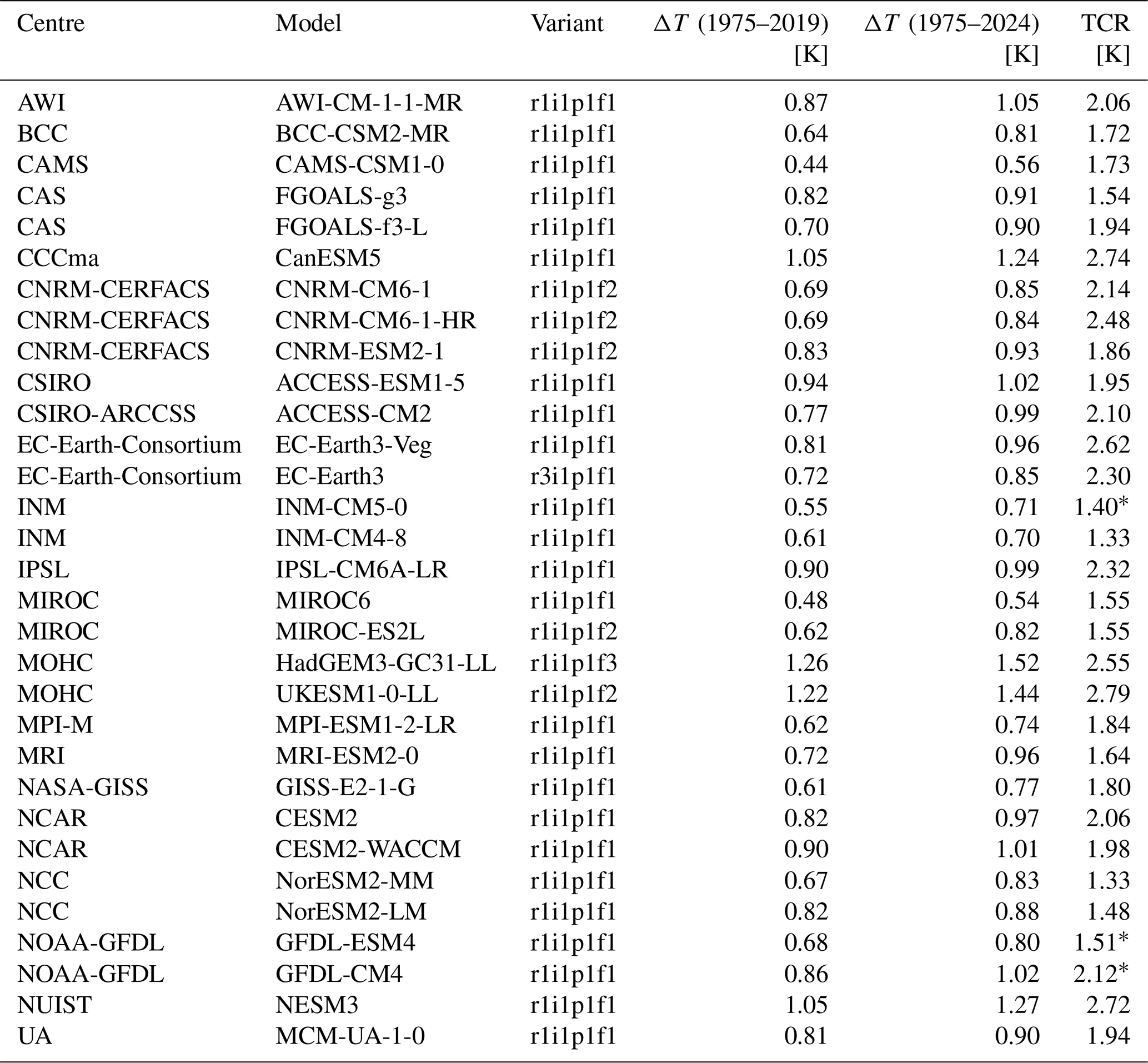
Table 1 List of CMIP6 ESMs used in this study. Models with an asterisk (^*) still met the criteria but did not have a TCR value given in the IPCC AR6 Chap. 7 appendix, and were therefore calculated directly using the piControl and 1pctCO2 experimental simulations.

There is ongoing debate about the validity of these high-sensitivity models. The emergent constraint technique aims to reduce such uncertainties by searching for an inter-ESM relationship between an aspect of future climate change and a measurable contemporary change in the real climate. Measurements of the current variable along with this regression can constrain the quantity associated with a future climate (Hall et al., 2019; Williamson et al., 2021). The TCR summary metric has proven more amenable to constraint than ECS, owing to its closer alignment with observed climate trends over the historical period, and because ECS by definition corresponds to a climate system in equilibrium, which is not presently the case. Studies that have constrained TCR using emergent constraint methods have consistently shown that high-sensitivity models are less consistent with historical warming (Jiménez-de-la Cuesta and Mauritsen, 2019; Tokarska et al., 2020; Nijsse et al., 2020). Nijsse et al. (2020) found that the most likely value of TCR is 1.7 ± 0.7 K (90 % confidence), which excludes the higher-sensitivity CMIP6 models. Tokarska et al. (2020) found a very similar estimate for TCR of 1.6 ± 0.4 K (66 % confidence), and went on to show that observationally-constrained warming projections tend to align more closely with the CMIP5 ensemble median than those from CMIP6 models.

In contrast, the true value of equilibrium climate sensitivity (ECS) remains a subject of active scientific debate. An assessment by Sherwood et al. (2020), which informed the ECS assessment in the IPCC AR6, constrained the range of effective climate sensitivity to between 2.3 and 4.5 K, with a best estimate near 3 K. This study found values below 2 K difficult to reconcile with historical observations, while, critically, values above 4.5 K were also considered unlikely (although not impossible). Paleoclimate studies examining past periods, such as the late Miocene, find evidence that is consistent with ECS values of around 4 K (Knutti et al., 2017; Sherwood et al., 2020; Brown et al., 2022). Constraints on ECS using observational records tend to be lower (Cox et al., 2018; Jiménez-de-la Cuesta and Mauritsen, 2019; Nijsse et al., 2020; Sherwood et al., 2020), with central estimates of ∼ 3 K. Future work that integrates overlapping ranges from multiple lines of evidence on the likely ECS could yield a more tightly constrained estimate of climate sensitivity (Sherwood et al., 2020).

Anthropogenic aerosol forcing continues to be a major source of uncertainty in climate sensitivity estimates. The net radiative effect of aerosols has been difficult to quantify due to their cooling effect and highly complex interactions with clouds. Models with strong aerosol cooling and high sensitivity can produce warming trajectories similar to those of models with weaker cooling and lower sensitivity (Andreae et al., 2005), making attribution challenging (Kiehl, 2007). Historically, global SO₂ aerosol emissions increased rapidly during the mid-20th century, peaking during the 1970s, before subsequently declining from 1980 onwards as a result of improved air quality regulations. This happened to coincide with rapid increases in greenhouse gas emissions, and this combined effect is thought to have contributed to the recent acceleration in observed warming (Samset et al., 2018; Hansen et al., 2025). Present-day estimates of aerosol effective radiative forcing lie between −1.6 and −0.6 W m⁻² (Bellouin et al., 2020), consistent with an inferred ECS of around 2.2 K (90 % range: 1.6–3.0 K), when accounting for pattern effects (Skeie et al., 2024). However, the influence of aerosols on cloud radiative feedback processes continue to be a major obstacle to constraining climate sensitivity. A recent study by Hansen et al. (2025) argues that the positive feedback associated with the albedo change suggests ECS values of 4.5 K, a level more consistent with paleoclimate based constraints rather than those constrained by observations over recent decades.

The recent observed warming has further emphasised the need to constrain estimates of climate sensitivity. The years 2023 and 2024 were the warmest on record, with 2024 marking the first time global temperatures exceeded 1.5 K above pre-industrial levels (HadCRUT5, NOAAGlobalTemp, ERA5, Berkeley Earth, Cannon (2025)). However, this short-term peak doesn't imply that the running mean of global warming has exceeded 1.5 K, as this surpassing coincided with a strong El Niño event during 2023 and 2024. It is suggested that such peaks due to ENSO may become more pronounced under climate change (Minobe et al., 2025). Nevertheless, the occurrence of these warm years, in addition to the larger TCR estimates from CMIP6 models in comparison to CMIP5, has raised questions regarding whether the Earth's climate sensitivity could in fact be greater than current estimates. This study uses updated observational data to refine the estimates of climate sensitivity produced by Nijsse et al. (2020), and to narrow the uncertainty in expected background levels of future warming for time-periods pertaining to the near future (2030), mid-century (2050) and late-century (2090) (Tokarska et al., 2020). We evaluate the extent to which the observed warming from 2020 to 2024 has influenced the likely ranges of TCR and future warming and compare these updated estimates with the likely ranges reported by the IPCC.

2 Methodology

To constrain TCR and future warming, we apply the emergent constraint procedure used by Nijsse et al. (2020) and Tokarska et al. (2020). The emergent constraint technique requires identifying an observable climate variable x that exhibits substantial variability within an ensemble of ESMs (such as CMIP6), and demonstrates a statistically significant relationship, f(x), with a target variable y. Since x is an observable quantity, it can be empirically determined from contemporary measurements. Consequently, f can be used to impose an observationally-informed constraint on y, based on the measurement of x. Such constraints are termed `emergent' because the relationship f arises from the collective behaviour of the model ensemble, and cannot be diagnosed from any individual climate model (Williamson et al., 2021). In this study, the climate observable x is defined as the change in a statistic of GMSAT relative to a specified baseline year, while the future climate variable y that we wish to constrain is either the TCR or projected future warming at a certain year.

Ideally, the emergent relationship between x and y should be supported by an underlying theoretical framework which characterises their association (Hall et al., 2019; Williamson et al., 2021). In this case, simple one- and two-box climate models (Gregory, 2000; Winton et al., 2010; Geoffroy et al., 2013; Caldeira and Myhrvold, 2013) provide a theoretical framework predicting a linear relationship between the change in GMSAT and both TCR and future warming (Jiménez-de-la Cuesta and Mauritsen, 2019; Nijsse et al., 2020; Tokarska et al., 2020). The relationship between TCR and the temperature anomaly ΔT is given by:

$$\begin{array}{}\text{(1)}& \text{TCR}=s\mathrm{\Delta }T+\mathit{\eta }\end{array}$$

where $s\equiv Q_{\mathrm{2}\times }/\mathrm{\Delta }Q$ is defined as the ratio of the radiative forcing associated with a doubling of CO₂, Q_2×, to the radiative forcing at the time of observation, ΔQ. For the purposes of model fitting, we include an intercept term η of the TCR axis to account for systematic biases, regression dilution and model misspecification.

Models that have demonstrated a stronger warming trend in the past are likely to simulate a greater warming in the future (Tokarska et al., 2020). Radiative forcing over the last 50 years has been dominated by the emission of greenhouse gases, and therefore, a similar linear relationship is also expected for future warming under the SSP scenarios:

$$\begin{array}{}\text{(2)}& \mathrm{\Delta }T\left(\text{Future}\right)=k\mathrm{\Delta }T\left(\text{Past}\right)+\mathit{\eta }.\end{array}$$

Here, k is the proportionality constant that relates past and future warming for each SSP scenario. For a period under which the warming rate is constant, the temperature difference over equal-length intervals should result in k=1. However, since ΔT is time dependent, we normalise ΔT(Past) per decade and use this as the observable. Thus, the ΔT(Future) is directly proportional to the $\mathrm{\Delta }T\left(\text{Past}\right)/\mathrm{10}\mathrm{yr}$, and the proportionality coefficient k will be scaled by 10yr, which can be interpreted as a decadal warming timescale.

2.1 Selection of ESM Simulations

We aimed to include as many CMIP6 ESMs as possible in the emergent constraint to maximise ensemble diversity. The selected models must include both a historical and at least one SSP simulation. Since the historical simulations end in 2014, the SSP simulations must fulfil the role of extending the historical run to the present day. As may be expected, we found that the ESM temperature projections exhibited only small differences between SSP scenarios during the 2015–2024 period, and therefore we adopted the SSP2-4.5 scenario by default for this interval. This selection is because the SSP2-4.5 scenario had the greatest number of ensemble members among the SSP scenarios. The final TCR prediction showed some variability depending on the choice of SSP scenario, with differences of approximately ± 0.04 K (see Supplementary Material, Sect. S2.2). For the analysis of future warming, the constraints were calculated individually for each SSP scenario. Therefore, our selected models needed a complete time series spanning the years 2015–2100 for the following four SSP scenarios: SSP1-2.6, SSP2-4.5, SSP3-7.0 and SSP5-8.5. While some models have explored additional scenarios (e.g., SSP1-1.9, SSP4-3.4), relatively few have simulated warming trends under these pathways. When possible, we chose the first ensemble member, labelled “r1ixpxfx”, which were available for 24 of the 31 models. As part of our robustness checks, 10 000 random permutations of ensemble members from all models were tested, and it was found that the final results remained largely invariant (Supplement Fig. S2).

2.2 Calculation of Warming Trend

Historical warming, the observable we used to constrain TCR and future warming from the SSP scenarios, is quantified as the difference in GMSAT between two smoothed periods, with each period averaged over a smoothing window to reduce the impact of internal variability. For example, the TCR constraint is based on the difference in GMSAT between 1975–1985 and 2014–2024. In order to constrain the future variables, the temperature trend between the two periods must exhibit a clear warming trend across all historical runs. The observational historical data show that global warming rose significantly from 1975; a trend captured by all runs across all models. A more rigorous analysis of the signal-to-noise ratio of the radiative forcing by Nijsse et al. (2020) (Fig. 5 in that paper) showed that it increased significantly from 1975, due to the increase in the forcing signal with no notable increase in noise. To assess the effect of the recent rapid warming observed since 2020 (most notably 2023 and 2024) on future variables, we extend the final year of the end period used by Nijsse et al. (2020) by 5 years, to include data up until 2024.

2.2.1 Accounting for Short-Term Internal Variability

To limit the effect of short-term (annual timescale) internal variability on the forced warming trend, we applied an equally-weighted, centred smoothing window to both ESM and observational GMSAT time-series. Varying the length of the smoothing window revealed that the final results remained largely unchanged for windows longer than 7 years (Supplement Fig. S1). Therefore following Nijsse et al. (2020), we chose an 11 year smoothing period so that our results were directly comparable. Tokarska et al. (2020) used a similar smoothing window of 10 years. This meant that the final data-point in the smoothed time series was centred around 2019 and spanned the 11-year period from 2014–2024. Although it might be expected that using a large smoothing window could obscure the influence of the exceptionally warm years of 2023 and 2024, it was found that reducing the window size to 5 years (with the final year being centred around 2022) did not result in a significant change in the final value of the TCR (Supplement Fig. S1).

Table 2 Emergent constraint of TCR comparison between non-extended and extended periods. Results from Tokarska et al. (2020) and Nijsse et al. (2020) are shown for comparison. Those results from Tokarska et al. (2020) and Nijsse et al. (2020), as well as this study, were extended using the SSP2-4.5 model runs. The distribution from the IPCC were obtained using the quoted likely ranges in Chap. 7 of IPCC AR6 (Forster et al., 2021).

Tokarska et al. (2020)Lee et al., 2021Lee et al., 2021

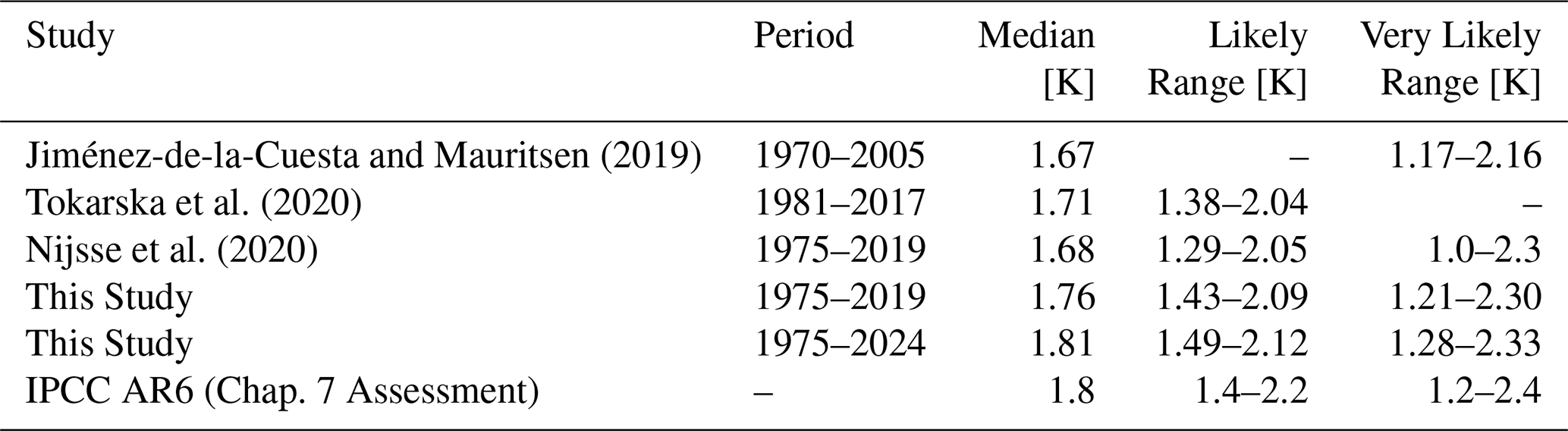
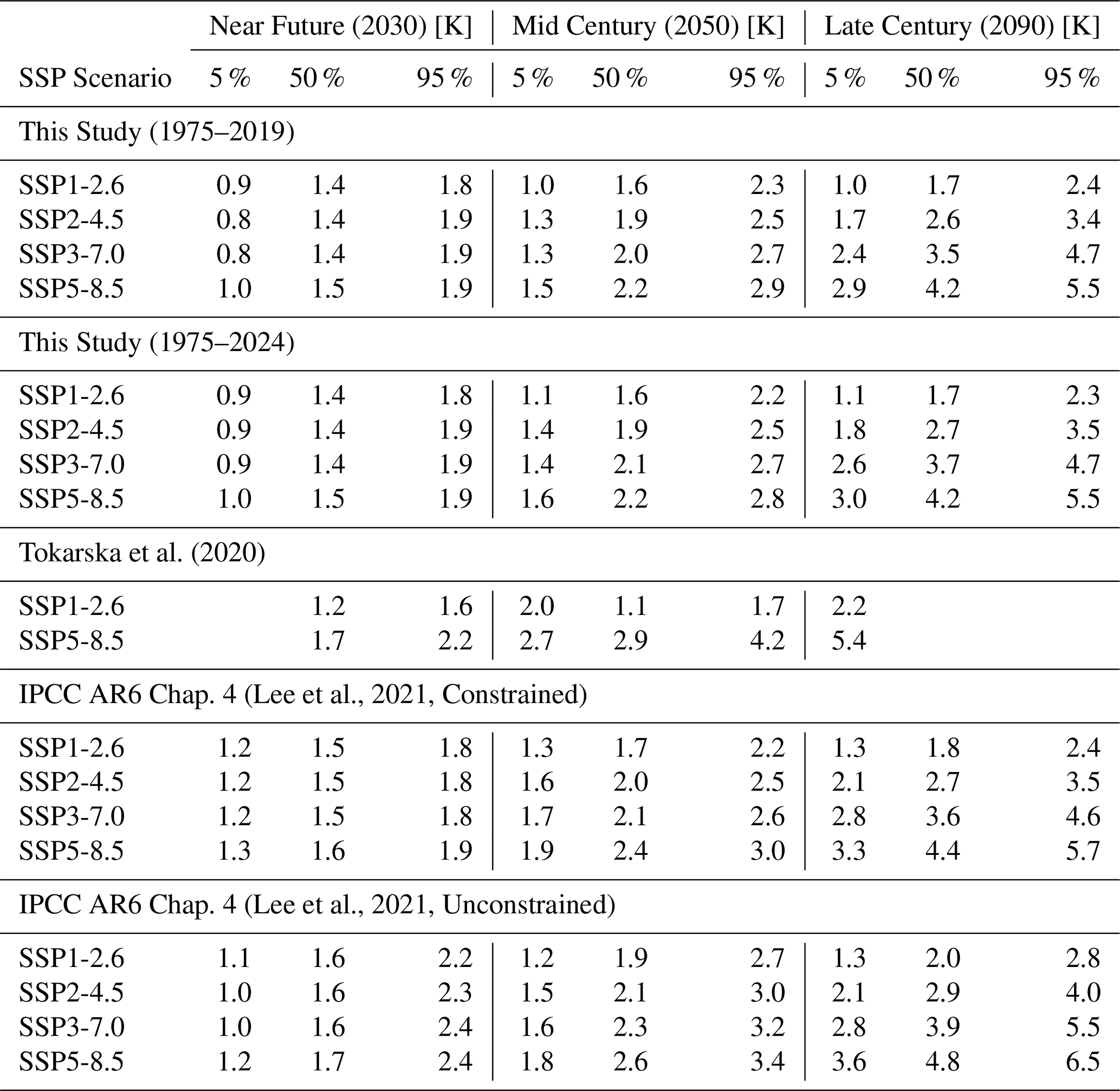
Table 3 Temperature anomaly estimates in the near future (centred 2030), mid-century (centred 2050) and late-century (centred 2090), constrained by the decadal warming rates from both 1975–2019, and 1975–2024. Anomalies are with respect to the pre-industrial mean (1850–1900). Shown are the central estimate and the 5 %–95 % confidence values. Near future, mid- and late-century anomalies from Tokarska et al. (2020) and the constrained and unconstrained estimates from the IPCC AR6 Chap. 4 (Lee et al., 2021, Tables 4.2 and 4.5) are shown.

2.2.2 Long-Term Internal Variability

Since we used the detrended historical runs to estimate the uncertainty in the forced warming trend, we exclude variability longer than the smoothing window. To assess the impact of this simplification, we examined GMSAT variability in unforced model control runs and compared it with that of the detrended historical runs (Supplement Sect. S3). For most ESMs, the estimates of internal variability are similar, although there is an expected tendency for GMSAT variability to be slightly larger in the un-detrended control runs. As a sensitivity test, we identified the largest fractional increase in GMSAT variability in the control runs and compared it with that of the detrended historical runs. This test was performed across the model ensemble and assessed the impact of variability on our emergent constraint on TCR. The uncertainty in the emergent constraint is dominated by the uncertainty in the emergent relationship, rather than the uncertainty in the observational constraint, and we therefore consider the latter to have a relatively small impact on our constrained ranges for TCR (see Sect. 4).

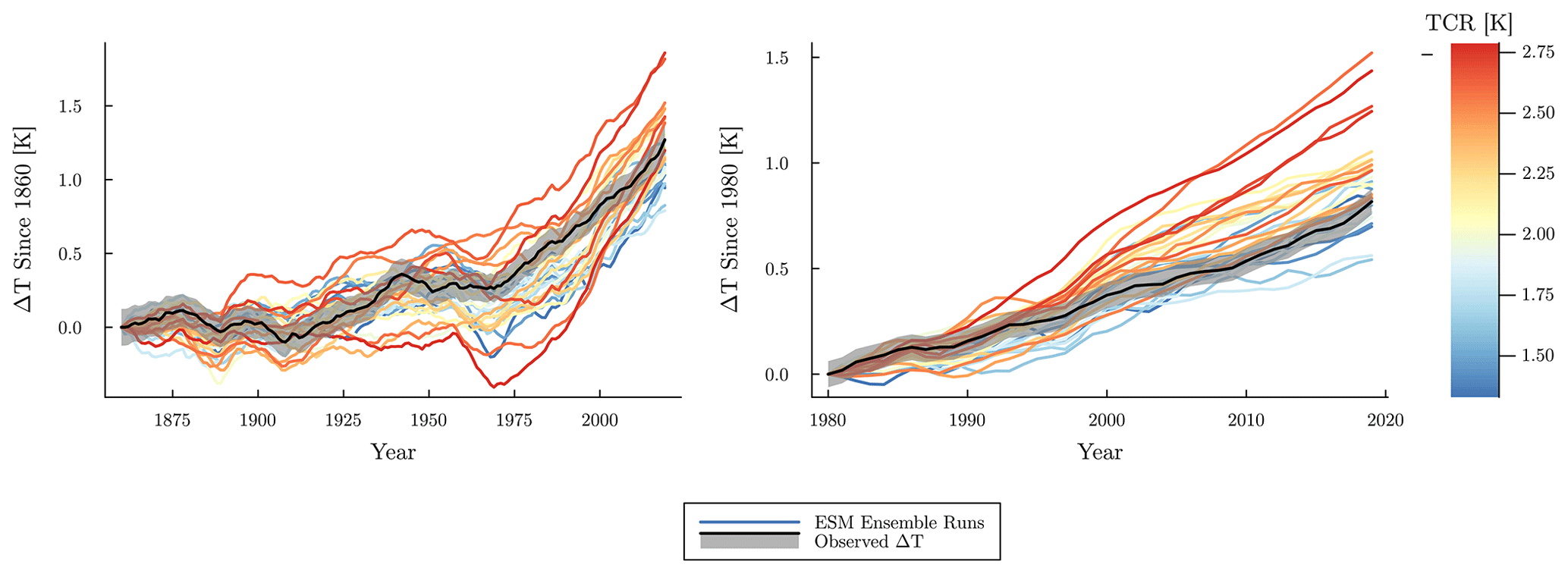
Figure 1 GMSAT anomaly time series of all available CMIP6 ESMs (n=31), with one ensemble member plotted per model. Years since 2014 have been extended using the SSP2-4.5 scenario. The models are coloured by their TCR value, with red indicating models with higher TCR and blue indicating lower TCR. The black dotted line in each case represents the observed warming averaged across all datasets over the same period, and the grey-shaded region represents the calculated observational uncertainty. All series are smoothed using a 11-year centred window. Left: Temperature Anomaly ΔT since the beginning of historical simulation period (1850), relative to the pre-industrial mean. Right: Temperature anomaly ΔT relative to the 1975–1985 mean.

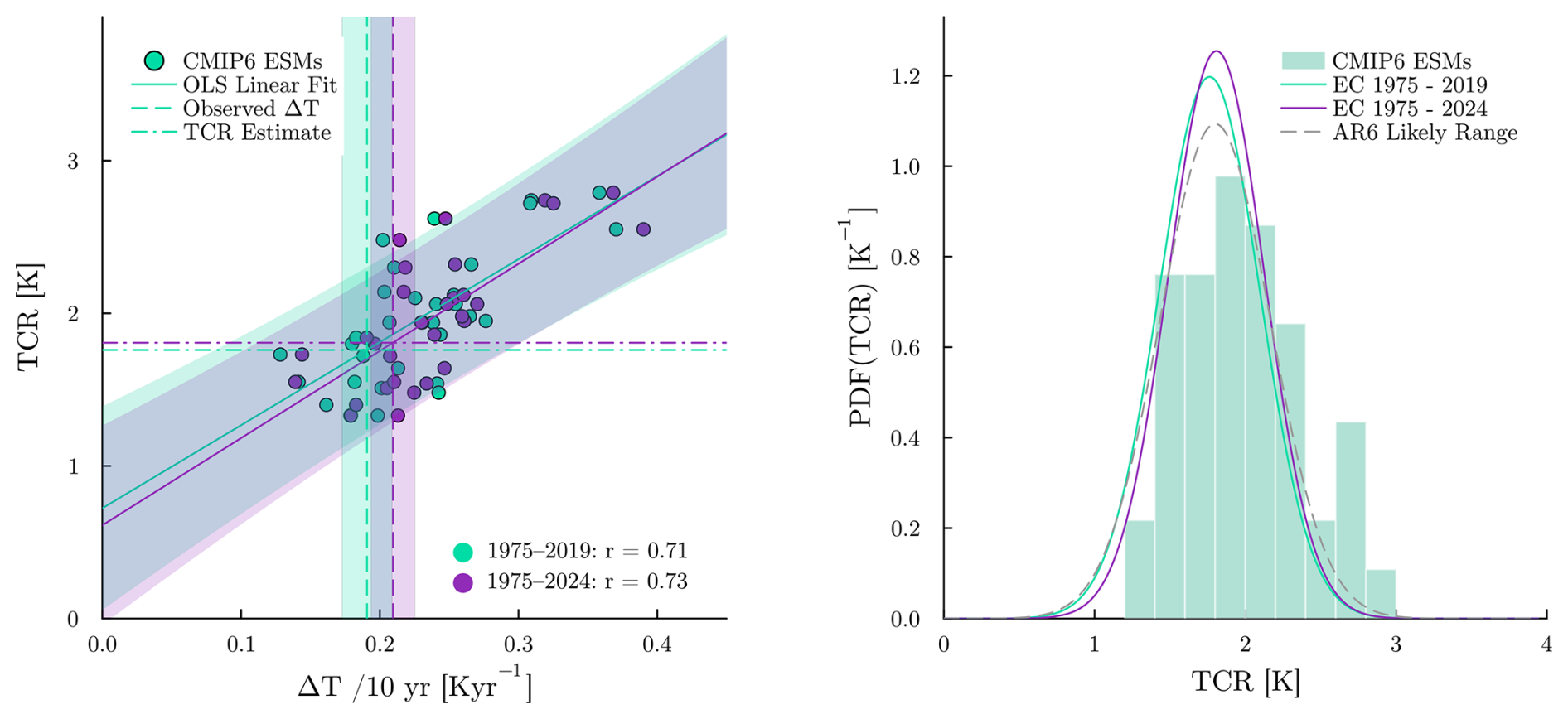
Figure 2 Left: Comparison between the emergent constraints on TCR against global warming, between the 2009 to 2019 end period (shown in green) and the 2014–2024 end period (shown in purple). The plotted quantity is the decadal warming rate, $\mathrm{\Delta }T/\mathrm{10}{\mathrm{yr}}^{-\mathrm{1}}$, which is calculated as the smoothed GMSAT using all years from 1975 to the respective end period, normalised by number of decades. OLS linear regression is performed using all available models (n=31). The shaded regions surrounding the regression lines indicate a 90 % prediction interval. The vertical dashed lines represent the mean value of the observations, with the shaded regions surrounding them representing the 95 % observational uncertainty (the uncertainty level quoted in the raw datasets). Right: Comparison of the PDFs for the TCR between the 2009–2019 end period and the 2014–2024 end period. These are shown in green and purple, respectively. For comparison, we provide the TCR estimate listed in Chapter 7 of the IPC6 AR6 (Forster et al., 2021). This PDF is based on the listed likely and very likely ranges, and is shown as a dotted line. Additionally, the raw CMIP6 model values are displayed as a histogram.

2.3 Calculation of Future Climate Variables

The variables we constrained in this analysis were TCR and ΔT in the future. We took TCR values from IPCC AR6 report as shown in Table 1. Additional values that were not reported, specifically for the models INM-CM5-0, GFDL-ESM4, and GFDL-CM4 (shown with an asterisk (^*) in Table 1), were also included in the analysis. These were calculated directly by evaluating the temperature difference between the control and 1pctCO2 simulations at the time when CO₂ has doubled from its initial concentration (approximately 70 years; Forster et al., 2021). For the calculation of ΔT in the future, we used the same method outlined in Sect. 2.2 to calculate the temperature difference between the start year and the end year. We selected a start year centred on 1980, and allowed the end year to be any point in the future. However, for comparison with both Tokarska et al. (2020) and the results in Chapter 4 of the IPCC AR6 (Lee et al., 2021), we chose 2030, 2050, and 2090 to represent the near-future, mid-century, and late-century years, respectively. To express all anomalies relative to the pre-industrial era, we applied an offset based on the temperature difference between the pre-industrial period (1850–1900) and the reference period (1975–1985). We note that the warming period used for the observable in the emergent constraint does not include the pre-industrial era, because, as discussed in Sect. 2.2, the assumption of a constant warming trend (and Eq. 2) is not valid over that interval. This definition is adopted only to ensure consistency with the IPCC.

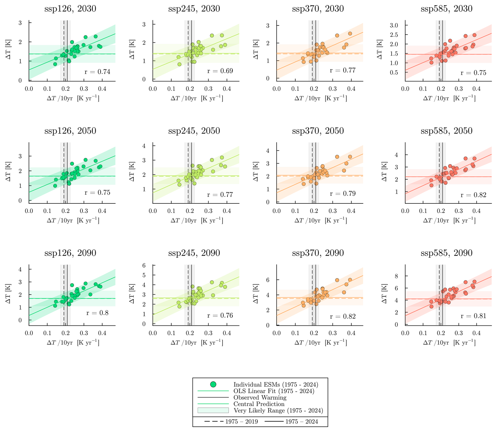
Figure 3 Emergent constraints on future warming using the observed decadal warming rate. Rows represent the three different end years, and columns represent the four available SSP scenarios (SSP1-2.6, SSP2-4.5, SSP3-7.0, SSP5-8.5). Future warming is with respect to the pre-industrial (1850–1900) baseline in all panels. The vertical lines in each panel represent the observed decadal warming, with the surrounding grey region showing the associated uncertainty. The horizontal lines show the central ΔT estimates using both the 1975–2019 and 1975–2024 warming rates as the constraint, and the surrounding shaded region indicates the very likely range for 1975–2024 constraint. In all cases, dashed lines represent the period 1975–2019, while solid lines represent 1975–2024. For clarity, only the ESM scatter points, linear fits, and likely range estimates for the 1975–2024 constraint are shown (a complete set of values is given in Table 3).

2.4 Constraining a Future Variable using Observational Data

2.4.1 Observational Data

This analysis used observational time series data from the following sources: HadCRUT5 (Met Office, Morice et al., 2021), Berkeley Earth (Berkeley, Rohde and Hausfather, 2020), GISSTemp (NASA, Lenssen et al., 2019), and GlobalTemp (NOAA, Huang et al., 2022). All anomalies in the raw dataset are relative to the pre-industrial mean (1850–1900). For estimates of TCR and future warming, we take an unweighted average of the anomaly at each year, across the four datasets. As with the time series from the ESMs, we apply an equivalent smoothing procedure, using an equally-weighted, centred smoothing window with an equivalent window length. The uncertainty of the forced warming signal in the observational datasets must also be included in the calculation of the emergent constraint. We include the uncertainty arising from two primary sources; the observational uncertainty in ΔT, and the short-term (annual) internal variability. The sources of observational uncertainty include incomplete spatial coverage and changes in measurement methods. The uncertainty associated with the short-term internal variability is estimated as the standard deviation of all points in time series (with respect to the smoothed series), divided by $\sqrt{n}$, where n is the number of points in the smoothing window. We also modify this to account for autocorrelation between adjacent years, which modifies n to an effective sample size, n_Eff, which decreases with increasing autocorrelation of the residual. The total uncertainty in the observations is calculated by taking the measurement and internal variability uncertainties in quadrature. For the chosen warming period of 1975–2024, the total observational uncertainty was found to be small relative to the spread across the ESMs.

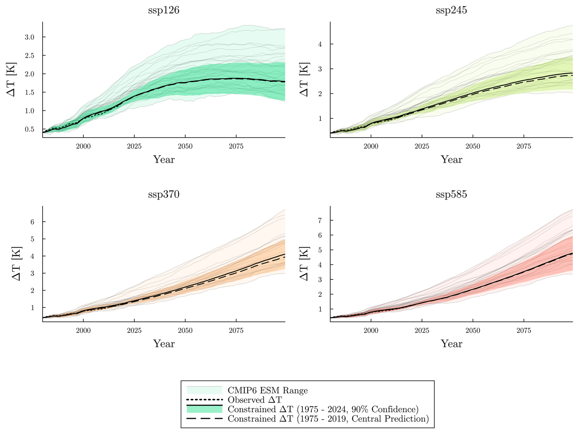
Figure 4 GMSAT anomaly time series under the four available SSP scenarios (SSP1-2.6, SSP2-4.5, SSP3-7.0, SSP5-8.5), relative to the pre-industrial (1850–1900) mean. Thin grey lines show individual ensemble runs; the light shaded area spans their full range. The dotted black line indicates the smoothed observed warming trend from 1975–2024. The darker shaded region shows the 90 % confidence range of constrained future warming using the period 1975–2024, while the solid black line shows this corresponding central prediction. For comparison, the dashed black line shows the central prediction obtained when the constraint is performed using the 1975–2019 warming trend; for clarity, only the central prediction is shown. All series are smoothed using a 11-year centred window.

2.4.2 Regression

To find our emergent relationship f(x), we used ordinary least squares (OLS) of the future variable y with the observable variable x. OLS was chosen for its simplicity, and because it has been found to lead to similar estimates to those obtained with more complex statistical approaches (Nijsse et al., 2020), Fig. 5. We combined this emergent relationship from the ESMs with the observed warming since 1975 to estimate TCR and future warming along with their uncertainty. The uncertainty is estimated using the approach given in the appendix of Cox et al. (2018), as well as in the Supplement (Sect. S1.2).

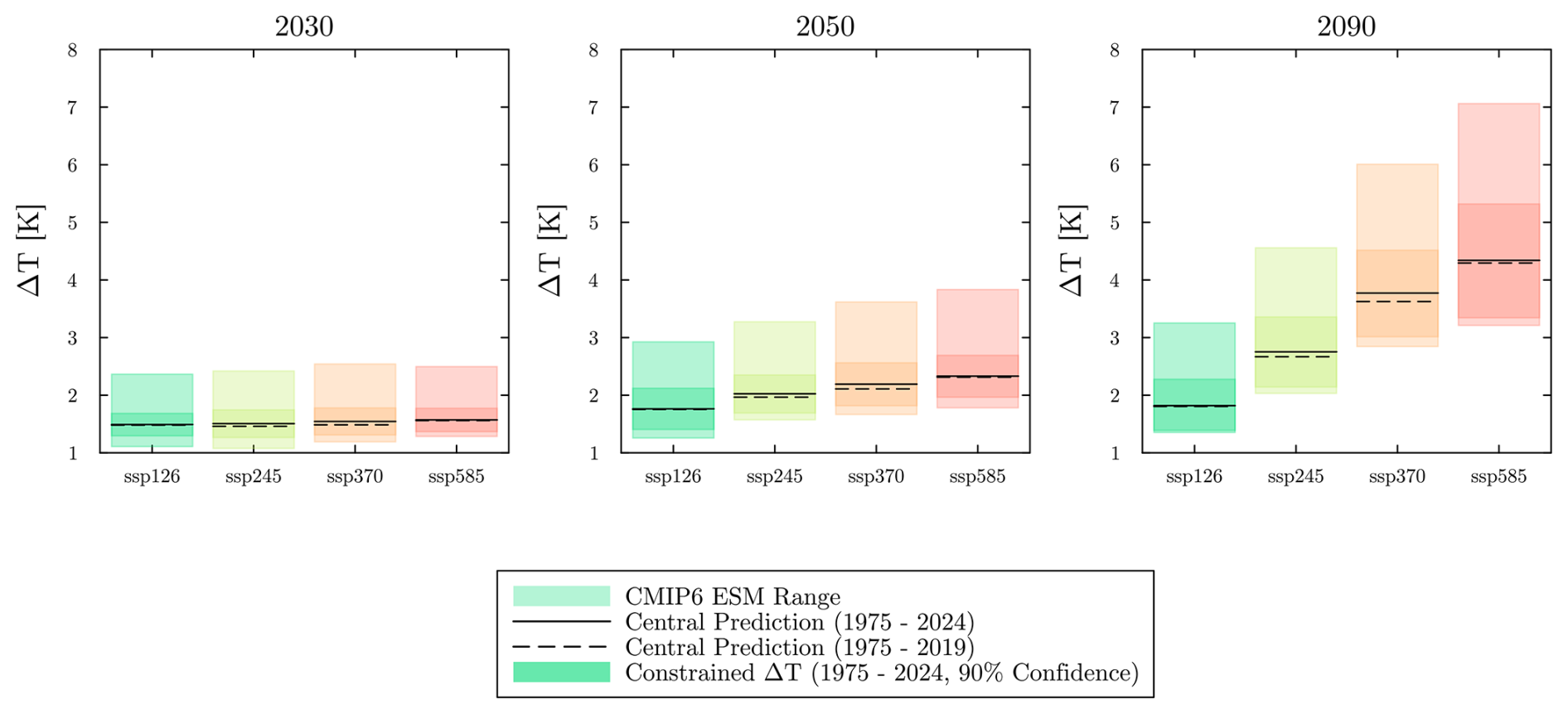
Figure 5 Comparison of the central estimates of the GMSAT prediction across the four available SSP scenarios (SSP1-2.6, SSP2-4.5, SSP3-7.0 and SSP5-8.5). The lighter coloured shaded regions represent the CMIP6 model ranges. The more saturated regions represent the constrained ranges at 90 % confidence, using the years from 1975–2024 as the constraint. Central predictions are shown as horizontal black lines; the solid line uses the 1975–2024 period as the constraint, while the dashed line uses the 1975–2019 period as the constraint. An 11-year smoothing period is used in all cases.

3 Results

3.1 TCR

We find a robust correlation between the predicted warming by individual ESMs and their TCR value. Figure 1 shows the average GMSAT anomaly of each model realisation. In total there were n=31 models that met the model selection criteria. As previously found by Nijsse et al. (2020), models with a high TCR value showed stronger than observed warming after 1975. Extending from 2019 to 2024 provides further verification of this correlation. Models with high TCR values (notably CanESM5, E3SM-1-0 and UKESM1-0-LL) show a strong warming in particular toward the end of the period.

Figure 2 compares the two PDFs of the TCR, based on the constraint derived from all CMIP6 ESMs (n=31), with and without the inclusion of the years 2020–2024. For comparison, the likely range quoted in the IPCC AR6 is also shown. All three distributions have very similar central estimates (all within < 0.05 K), with only a slight increase in the central prediction with the inclusion of the years 2020–2024. Additionally, there is a slight tightening of the distribution when the years 2020–2024 are included, likely due to the increased length of the warming period. The values of the TCR predictions along with the likely ranges are included in Table 2.

3.2 Constrained Future Warming in the SSP Scenarios

The high correlation between warming from ESMs and climate sensitivity provides a strong indication that observed past warming is correlated with future warming. Consistent with previous studies which used a similar methodology (Nijsse et al., 2020; Tokarska et al., 2020), we find a strong correlation between a model's warming from recent years, and the predicted future temperature in the various SSP scenarios.

We find a constraint on the projected temperature anomaly, ΔT, for mid-century and end-of-century values relative to the pre-industrial (1850–1900) baseline (y axis variable). The observable variable (x axis variable) for this emergent constraint is the decadal warming rate since 1975 (Tokarska et al., 2020).

Table 3 provides a summary of constrained temperature anomaly estimates for each SSP scenario in the near future, mid-century and late-century. Across all scenarios, our central estimates and very likely ranges remain close to that of the IPCC AR6. For instance, in the SSP5-8.5 scenario, the late-century central estimate is 4.3 K in this study, compared to 4.4 K in the IPCC AR6 constrained estimate. While the mid- and late-century projections are highly dependent on the SSP scenario, we find that near-future projections are consistent across scenarios.

Figure 3 is a graphical representation of Table 3's emergent constraint plots, stratified by both SSP scenario and year. The strength of the correlation varies according to the choice of SSP scenario and end year, with correlation coefficients varying from 0.66 to 0.81.

In Fig. 4 we show time-continuous emergent constraints on the likely ranges of warming in each of the SSP scenarios. These constraints use the warming trend over the years from 1975–2024 for the observable (as with the TCR constraint), with warming at some specified year in the future SSP scenario as the y axis variable.

Across all four SSP scenarios, the observationally-constrained central estimate lies within the low to mid region of the model range, which is in accordance with the observational trend line. An alternative representation of the same constraint is shown in the form of a bar plot in Fig. 5. This compares the constrained estimates across SSP scenarios for all three end years. This once again shows that all constraints lie within the low to mid region of the model range, and that the prediction in the near future (2030) is largely independent of the SSP scenario.

4 Discussion

The emergent constraint on the TCR produced in this analysis is largely in agreement with the central TCR estimate of the IPCC AR6 Chapt. 7, but is slightly larger (by ∼ 0.1 K) than that of Jiménez-de-la Cuesta and Mauritsen (2019), Nijsse et al. (2020) and Tokarska et al. (2020). The likely range in TCR in our analysis was narrower than that of both Nijsse et al. (2020) and Tokarska et al. (2020), and is very similar to that of Jiménez-de-la Cuesta and Mauritsen (2019) as well as the IPCC AR6 Chap. 7. The increase in the central estimate when evaluated using observational data from 1975 to 2019 and 1975 to 2024 is less than the difference between the central estimates in this study to both Nijsse et al. (2020) and Tokarska et al. (2020). The primary reason for this discrepancy is that the observational temperature anomaly datasets used in this study differ sufficiently to affect the calculation. As noted by Morice et al. (2021), the HadCRUT5 dataset includes upward revisions to temperature anomalies relative to its predecessor HadCRUT4, particularly after the start of the 21st century. These revisions lead to a increased observed warming trend in comparison to Nijsse et al. (2020) and Tokarska et al. (2020) and, consequently, a higher estimated TCR. Since HadCRUT4 has now been superseded by HadCRUT5, it was not used in this study. The differences between the two datasets are likely a result of using updated sea and land temperature measurement techniques, more sophisticated statistical methods to fill observational gaps, and a revised uncertainty evaluation for certain past years. This highlights a degree of sensitivity inherent to the emergent constraints approach, as it's highly dependent on robust observational data.

An additional reason for the discrepancy arises from the difference in the choice of model realisation compared to that of Nijsse et al. (2020). The approach in this study simply used one ensemble member run per model, the one which had a prescribed set (r1ixpxfx) of initialisation conditions (available in all ESMs with the exception of the EC-Earth3 model). The hierarchical Bayesian approach used in Nijsse et al. (2020) allowed different realisations to be combined into the overall fit. However, the same study showed that it gave nearly identical uncertainty ranges to the method using one ensemble member and OLS. A third source of the discrepancy arises from differences in the time periods used to derive the constraint. This study uses all years from 1975–2024 compared to those used in Nijsse et al. (2020) and Tokarska et al. (2020), which considered 1975–2019 and 1981–2017, respectively. Evaluating warming over a longer time period allows for a clearer trend to emerge, provided that the warming continues in a manner consistent with those previous years.

An additional source of uncertainty in our emergent constraints is the spatial pattern effects of sea surface temperatures (SST), whereby this effect potentially weakens the relationship between observed warming and climate sensitivity (and hence future warming) (Wills et al., 2022; Alessi and Rugenstein, 2023; Armour et al., 2024). However, studies have shown that the magnitude of emergent bias depends on the choice of SST dataset and the boundary conditions used to drive the forcing (Andrews et al., 2022; Modak and Mauritsen, 2023). Most analyses of the pattern effect have primarily focused on ECS (rather than TCR), which quantifies climate sensitivity under very long timescales.

As mentioned in Sect. 2.2.2, our comparison of the internal variability between the pre-industrial control runs and the detrended historical runs suggests that our estimate of internal variability in the detrended observational time series could be underestimated, by up to a maximum factor of ∼ 2.7 (Supplement Sect. S3, largest model ratio for CNRM-CM6). Multiplying our observational uncertainty due to internal variability by this factor causes a slight broadening of the likely TCR range. We find that our 90 % confidence range of TCR would change from 1.28–2.33 K to a maximum range of 1.18–2.42 K, for the model with this most extreme ratio of control to historical temperature variability. This small impact to such a large increase in the assumed uncertainty in the observed warming trend is because the uncertainty in the emergent constraint on TCR is predominantly due to the uncertainty in the emergent relationship across the models, rather than the uncertainty in the variability of the observed warming trend.

The emergent constraints on the future temperature anomalies since the pre-industrial era by mid-century and late-century are, unsurprisingly, largely in agreement with those of Tokarska et al. (2020) as well as that of Chap. 4 of the IPCC AR6 (Lee et al., 2021). The observable used to produce the emergent constraint in both this study and Tokarska et al. (2020) was the decadal warming rate, whereas that of IPCC AR6 was derived by combining scenario projections, observational constraints, and updated assessments of ECS and TCR. As shown in Fig. 4, the central estimate of the future warming projection is consistently within the low to mid part of the model range.

5 Conclusions

It is likely that the 1.5 °C warming level as set out by the 2015 Paris agreement will be exceeded within the next 10 years, given the recent warming trend (Cannon, 2025), and the failure to reduce global CO₂ emissions in line with the lower forcing scenarios SSP1-1.9 and SSP1-2.6 (Friedlingstein et al., 2025). However, our results show that, for both TCR and future warming, the record global warming of 2023 and 2024 does not justify upward-revision of likely ranges. Therefore, the constraints presented here suggest that avoiding 2 °C of global warming, although challenging, remains possible.