Quantifying resilience in non-autonomous and stochastic Earth system dynamics with application to glacial-interglacial cycles

Understanding Earth resilience – the capacity of the Earth system to absorb and regenerate from perturbations – is key to assessing risks from anthropogenic pressures and sustaining a safe operating space for humanity within planetary boundaries. Classical resilience indicators are designed for autonomous systems with fixed attractors, but the Earth system is fundamentally non-autonomous and out of equilibrium, calling for new ways of defining and quantifying resilience.

Here, we introduce a path-resilience approach that assesses how perturbations deviate from and return to a reference trajectory of a conceptual climate model replicating the glacial-interglacial cycles of the Late Pleistocene. We generate two types of perturbation ensembles: a stochastic ensemble and a pulse-perturbation ensemble, and compute two complementary metrics: the Reference Adherence Ratio, RAR(t), defined as the fraction of stochastic trajectories that remain within a narrow band around the unperturbed trajectory; and return time, defined as the time a single perturbed trajectory takes to return to the reference path. Together, these metrics reveal strong temporal variation in resilience across the glacial-interglacial cycles. We find that RAR(t) increases markedly during deglaciations and peaks in interglacial periods, while return times generally shorten as the system approaches interglacial conditions, indicating that certain phases of the cycles act as convergence zones along the forced trajectory. As the Earth system departs from such interglacial regimes under ongoing anthropogenic forcing, understanding the resilience of these trajectories, and what it may take to return to them, becomes increasingly important.

These results highlight that resilience in non-autonomous systems is inherently path-dependent and illustrate a promising first step toward its quantification. Further research is needed to develop more general resilience indicators suitable for complex, forced dynamical systems.

1 Introduction

Quantifying Earth system resilience is essential for evaluating the planet's capacity to withstand and regenerate from growing human-induced stresses, such as greenhouse gas emissions and land-use changes (Rockström et al., 2021; Anderies et al., 2023). As humanity continues to transform the climate system and the biosphere, understanding the processes that strengthen or undermine its stability becomes increasingly important (Yi et al., 2024). Such knowledge is crucial for developing strategies to regenerate and reinforce Earth system resilience, ultimately helping society return to a safe operating space within planetary boundaries (Richardson et al., 2023; Caesar et al., 2024; Folke et al., 2010).

The concept of resilience has been explored from multiple disciplinary perspectives, giving rise to diverse definitions. Two predominant forms have traditionally defined the field: engineering resilience (Holling, 1996), which concerns linear stability analysis and the rate of return to equilibrium after small perturbations, and ecological resilience, which addresses the resilience of nonlinear dynamical systems with multiple stable states and their capacity to maintain essential functions while transitioning between different regimes (Holling, 1973). Related terms such as stability, robustness, and persistence are often used interchangeably despite subtle differences, creating definitional diversity that has spread across social and natural sciences (Krakovská et al., 2024; Anderies et al., 2013). To navigate this complexity, the question of resilience of what to what? (Holling, 1973; Tamberg et al., 2022) has become a guiding framework – clarifying which system components are meant to be sustained, which properties are at risk, and which disturbances are relevant. Here, this question is interpreted as the resilience of the glacial-interglacial ice volume trajectory to perturbations, i.e., the capacity of the ice-climate-carbon system to remain close to its characteristic large-scale path in face of external shocks.

This framework gains particular relevance when examining Earth's climate history. Palaeoclimate variability during the Cenozoic offers important insights into the Earth system's changing stability and resilience, as there is evidence for alternative attractors (Westerhold et al., 2020) and resilience loss before major climate shifts and hyperthermal events in that period (Setty et al., 2023).

Building on this palaeoclimate context, the glacial-interglacial cycles of the Late Pleistocene offer a compelling test case for studying Earth system resilience, due to their regularity and sensitivity to external forcing (Milankovitch, 1920; Lisiecki and Raymo, 2005). These cycles involve transitions between long glacial periods with large continental ice sheets and shorter interglacials with reduced ice volume, paced by variations in Earth's orbital configuration – eccentricity, obliquity, and precession – which act faster than the system's internal adjustment times. The dominance of the ∼ 100 000-year cycle in the Late Pleistocene, despite weak direct insolation forcing at that frequency, poses a long-standing puzzle in palaeoclimate dynamics (Imbrie et al., 1993), with a variety of proposed solutions (e.g., Willeit et al., 2019; Abe-Ouchi et al., 2013). The Earth system can thus be viewed as a non-equilibrium, externally forced system, following a quasi-periodic trajectory shaped by the interplay between astronomical forcing and internal feedbacks.

Over the past 800 000 years, this glacial-interglacial rhythm has been remarkably persistent (Lisiecki and Raymo, 2005). However, model studies suggest that anthropogenic greenhouse gases already present in the atmosphere may delay the next glacial inception by over 100 000 years (Ganopolski et al., 2016), marking a significant departure from the quasi-periodic limit cycle that has dominated recent Earth history. Continued warming raises the risk of a further shift toward ”Hothouse Earth” conditions that last occurred millions of years ago, conditions that modern human societies would likely be unable to adapt to (Steffen et al., 2018; Kaufhold et al., 2025). The resilience of Holocene-like interglacial states, which define the safe operating space delineated in the planetary boundary framework (Rockström et al., 2024), must therefore be understood within a non-equilibrium framework, as such interglacial states naturally occur as part of a dynamically evolving glacial-interglacial cycle. Observational evidence already hints at systemic weakening, including reduced carbon sink capacity in land-systems (Ke et al., 2024) particularly in the Amazon (Brienen et al., 2015; Gatti et al., 2021), and amplified feedbacks in the ocean-atmosphere system and other tipping elements (Wunderling et al., 2024). While this study does not address such future scenarios directly, they underscore the need to understand Earth system resilience.

Classical resilience indicators – such as return time to equilibrium, eigenvalue-based stability measures, or potential well depth – are poorly suited for systems like the glacial-interglacial cycle. These metrics are typically developed for autonomous systems with fixed-point attractors and assess resilience as the rate of return to such a state after perturbation (Krakovská et al., 2024). The Earth system, by contrast, is fundamentally non-autonomous, driven by time-dependent forcings such as orbital variations and, more recently, anthropogenic influences. These drivers operate on shorter timescales than the system's intrinsic adjustment times, resulting in transient dynamics that do not converge to equilibrium. Consequently, conventional indicators fail to meaningfully characterise resilience in this context.

Related approaches have nevertheless been used to study transient stability in glacial-cycle dynamics, including finite-time Lyapunov exponents, potential analysis, and early-warning-signal methods (De Saedeleer et al., 2013; Mitsui and Crucifix, 2016; Livina et al., 2011; Dakos et al., 2008). These approaches provide complementary perspectives on transient stability. In this study, we use finite-time Lyapunov exponents as a comparison diagnostic (Fig. 3), while our main focus is on how finite perturbations deviate from and return to a time-dependent reference path under identical forcing.

Against this background, we adopt a path resilience perspective (Anderies et al., 2023). Rather than asking whether the system returns to a stable state, the focus here is on how perturbed trajectories deviate from – and eventually return to – a reference trajectory. In this framing, the path itself becomes the object of resilience analysis, making it more appropriate for externally forced, non-equilibrium systems. Returning to the “resilience of what to what?” framework, resilience is defined here as the resilience of the glacial-interglacial ice volume trajectory to perturbations in ice volume, with the “sustainant” being the historical reference trajectory, and the “disturbance” being imposed stochastic variability or pulse-like shocks, representing internal variability and external shocks respectively.

In this study, we employ a reduced-complexity climate model developed by Talento and Ganopolski (2021). The model captures essential large-scale feedbacks among global ice volume, atmospheric CO₂, and global mean temperature. Its low dimensionality makes it computationally efficient and particularly suitable for long-term ensemble simulations designed to explore dynamical behaviour under perturbations. Our goal is not to produce detailed predictions, but to develop and demonstrate a transparent methodology for measuring path-wise Earth system resilience that can be extended to more complex models.

We generate two perturbation ensembles: a stochastic ensemble with low-amplitude continuous noise, following the Hasselmann framework (Hasselmann, 1976), to represent unresolved fast processes; and a pulse-perturbation ensemble, in which the system is shocked once at a selected time point and then allowed to evolve deterministically. We apply two main diagnostics: the Reference Adherence Ratio, RAR(t), which measures how closely perturbed trajectories follow a reference path over time; and the return time, which quantifies how long it takes trajectories to rejoin and remain near the reference. In addition, we compare these path-resilience metrics with a finite-time Lyapunov exponent diagnostic following Mitsui and Crucifix (2016). Together, the two main diagnostics operationalise path resilience in a non-autonomous dynamical systems setting.

The paper is organised as follows: Sect. 2 describes the model setup and governing equations; Sect. 3 introduces the perturbation ensembles and resilience metrics, and presents the results; Sect. 4 discusses model limitations and their implications; and Sect. 5 summarises the main conclusions and outlines future directions.

2 Model setup

This section describes the reduced-complexity climate model of Talento and Ganopolski (2021) used to simulate glacial-interglacial dynamics on orbital timescales. The model represents the co-evolution of three globally averaged variables: ice volume anomaly v(t), atmospheric CO₂ concentration CO₂(t), and global mean temperature anomaly T(t). In our implementation, the model is treated as a differential-algebraic system: v(t) is the only prognostic variable, advanced by a single first-order integro-differential equation for ice-sheet evolution, while CO₂(t) and T(t) are diagnosed from algebraic closure relations at each time step.

The model is explicitly non-autonomous, with time-dependent orbital forcing as the sole external driver. Internal feedbacks include the ice-albedo effect, dynamic carbon cycle responses, and a memory term reflecting the persistence of ice sheets over multi-millennial timescales. These mechanisms jointly enable the model to reproduce key features of Quaternary glacial variability, such as the characteristic asymmetric ice volume cycles.

The model is governed by three coupled equations. The global ice volume evolution is described by:

$$\begin{array}{}\text{(1)}& {\displaystyle \frac{\mathrm{d}v}{\mathrm{d}t}}={\displaystyle \frac{b_{\mathrm{1}}v-b_{\mathrm{2}}{v}^{\mathrm{3}/\mathrm{2}}-b_{\mathrm{3}}(f-\stackrel{\mathrm{‾}}{f})-b_{\mathrm{4}}\log \left({\mathrm{CO}}_{\mathrm{2}}\right)}{\mathrm{1}-b_{\mathrm{5}}{M}_{\mathrm{v}}}}+b_{\mathrm{6}},\end{array}$$

where $f\left(t\right)-\stackrel{\mathrm{‾}}{f}$ is the anomaly of the time-dependent orbital forcing index relative to its long-term mean, log denotes the natural logarithm, and M_v(t) a memory term that accounts for the integrated ice volume over the past τ=30 kyr:

$$\begin{array}{}\text{(2)}& M_{\mathrm{v}}\left(t\right)=\left\{\begin{array}{ll}\frac{\mathrm{1}}{\mathit{\tau }}{\int }_{t-\mathit{\tau }}^{t}v\left(x\right)\mathrm{d}x& \text{if }\frac{\mathrm{d}v}{\mathrm{d}t}<\mathrm{0},\\ \mathrm{0}& \text{otherwise.}\end{array}\right.\end{array}$$

This term plays a key role in reproducing the asymmetric shape of the glacial cycles by accelerating ice volume collapse during deglaciations. The memory timescale τ=30 kyr, adopted from Talento and Ganopolski (2021), is consistent with the typical lithospheric adjustment time to ice sheet loading. Ice volume anomaly v is unitless and normalised to zero at pre-industrial levels and unity at the last glacial maximum.

Atmospheric CO₂ concentration (in units of ppm) is determined by:

$$\begin{array}{}\text{(3)}& {\mathrm{CO}}_{\mathrm{2}}=c_{\mathrm{1}}T+c_{\mathrm{2}}v+c_{\mathrm{3}}min\left({\displaystyle \frac{\mathrm{d}v}{\mathrm{d}t}},\mathrm{0}\right)+c_{\mathrm{4}}+{\mathrm{Anth}}_{{\mathrm{CO}}_{\mathrm{2}}},\end{array}$$

where c₄=278 ppm is fixed to represent pre-industrial CO₂ levels, and ${\mathrm{Anth}}_{{\mathrm{CO}}_{\mathrm{2}}}$ captures externally imposed anthropogenic emissions. In this study, we focus on natural dynamics and set ${\mathrm{Anth}}_{{\mathrm{CO}}_{\mathrm{2}}}=\mathrm{0}$.

Finally, global mean temperature anomaly (in units of K) is given by:

$$\begin{array}{}\text{(4)}& T=d_{\mathrm{1}}v+d_{\mathrm{2}}\log \left({\displaystyle \frac{{\mathrm{CO}}_{\mathrm{2}}}{\mathrm{278}}}\right),\end{array}$$

where the first term represents the ice-albedo effect, and the second captures the greenhouse effect of CO₂ approximated by its logarithmic dependence on concentration relative to the pre-industrial baseline.

Figure 1 compares the simulated ice-volume anomaly with the palaeo-reconstructed global ice-volume anomaly derived from the sea-level stack of Spratt and Lisiecki (2016), along with the imposed orbital forcing and frequency spectra. Using a model calibration as described in Sect. 2.2, the model captures both the amplitude and dominant periodicities of Quaternary glacial cycles reasonably well, making it a solid basis for the perturbation experiments in this study.

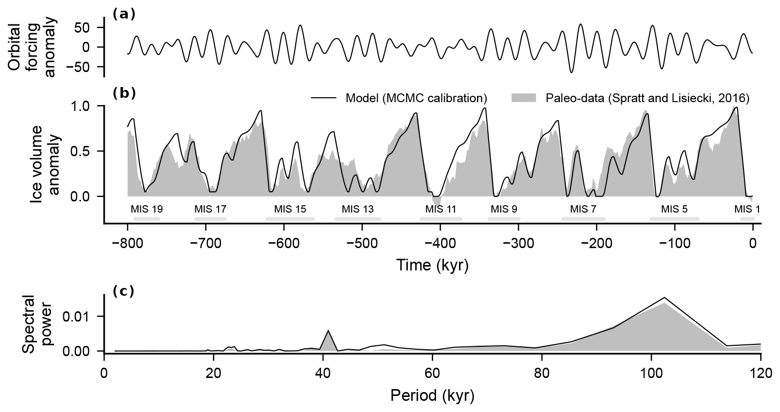
Figure 1 Model validation against a palaeo-reconstruction of global ice-volume anomaly over the past 800 kyr. (a) Anomaly of the orbital forcing index, $f\left(t\right)-\stackrel{\mathrm{‾}}{f}$, where f(t) is the Talento and Ganopolski 65° N summer-insolation proxy constructed from climatic precession and obliquity. (b) Simulated ice-volume anomaly compared to the global ice-volume anomaly reconstructed from the sea-level stack of Spratt and Lisiecki (2016), with Marine Isotope Stage (MIS) interglacial boundaries marked. (c) Frequency spectra of the simulated and reconstructed ice-volume anomalies.

In the model, f(t) is not direct summer-solstice insolation at 65° N, but the Talento and Ganopolski orbital forcing index: a 65° N summer-insolation proxy constructed from obliquity obl(t) and climatic precession pre(t) following Jackson and Broccoli (2003). Talento and Ganopolski decomposed the forcing into these two components and recombined them into a scaled linear combination:

$$\begin{array}{}\text{(5)}& f\left(t\right)=\mathrm{pre}\left(t\right)+\mathit{\gamma }\left(\mathrm{obl}\left(t\right)-\langle \mathrm{obl}\rangle \right),\end{array}$$

with γ=1.04 optimised to maximise the correlation with the critical CO₂ threshold. In our implementation, pre(t) and obl(t) are the forcing series provided in the Talento and Ganopolski data files smx_p.mat and smx_o.mat (Talento, 2021). These series are already on an insolation-like scale, so we use them without additional scaling or normalisation. The only preprocessing applied is the mean subtraction shown in Eq. (5), through the term $f\left(t\right)-\stackrel{\mathrm{‾}}{f}$. The mean orbital forcing $\stackrel{\mathrm{‾}}{f}$ entering the ice volume equation is computed over the full 2000 kyr forcing time series, i.e. the $[-\mathrm{1000},+\mathrm{1000}]$ kyr window.

2.1 Model constraints and limitations

Like all reduced-complexity models, this model employs simplifying assumptions and explicit constraints. These choices are detailed in the original study by Talento and Ganopolski (2021), but we briefly highlight two constraints that are important for this work.

The most important constraint for our resilience analysis is that global ice volume is constrained not to fall below its pre-industrial level (v≥0), reflecting the present-day as the zero anomaly baseline. This approach leads to interglacials being represented by extended periods of zero ice-volume anomaly, which does not fully capture the gradual transitions seen in palaeoclimate data. This artificial boundary may create an illusion of enhanced stability during interglacial periods, as perturbed trajectories cannot deviate below this constraint.

The model also imposes a constraint to simulate the mid-Brunhes transition, a shift around 400 kyr BP after which interglacials became notably stronger. This change is not well explained by orbital forcing alone and is likely linked to external factors not captured by the model. To approximate this behaviour, ice volume is not allowed to fall below 0.05 before 400 kyr BP. This, however, introduces a sharp drop from 0.05 to 0 at the time of the transition, which does not realistically reflect the gradual nature of the transition.

2.2 Numerical implementation

Talento and Ganopolski (2021) originally implemented the model in Matlab. We re-implemented it in Python and integrated it using a forward Euler scheme with a time step of Δt=1 kyr, consistent with the original study. At each time step, we first diagnose T(t) from the previous-step ice volume and atmospheric CO₂, then diagnose CO₂(t) from T(t), the previous-step ice volume, and a backward-difference estimate of $\mathrm{d}v/\mathrm{d}t$, and finally advance v(t) by one time step using the ice-volume equation. The memory term M_v(t) is calculated using a trapezoidal approximation of the integral over the past 30 kyr. This numerical setup provides sufficient accuracy to reproduce key features of glacial-interglacial cycles while remaining computationally efficient for ensemble experiments. To reduce the influence of initial transients before comparison with palaeo data, each simulation is extended by 200 kyr prior to the start of the observational window.

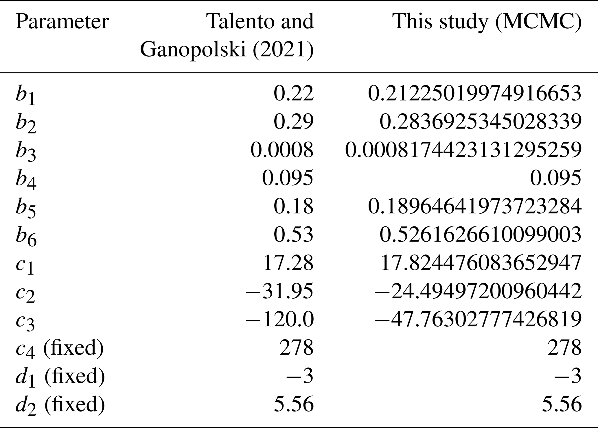
To calibrate the model's nine tuneable parameters, we employed a Metropolis-Hastings Markov Chain Monte Carlo (MCMC) approach. We follow the original calibration strategy and optimise the model ice volume output by comparing it against reconstructed ice volume anomalies from the Spratt and Lisiecki (2016) sea-level stack spanning the past 800 kyr, and obtain a Pearson correlation coefficient of 0.892 with the reconstruction. Notably, the parameters c₂ and c₃, which govern the sensitivity of CO₂ to ice volume and its rate of change (Eq. 3), differ substantially from the original values. This may reflect structural differences in implementation or sensitivity in the calibration process. Further details on the MCMC setup and likelihood function are provided in Appendix A.

3 Perturbation experiments and indicators of path resilience

3.1 Experiment I: Stochastic ensemble and Reference Adherence Ratio (RAR)

To investigate the resilience of the glacial-interglacial trajectory under persistent, small-scale disturbances (e.g. representing internal variability), we extend the model with a stochastic noise component and analyse its effect on an ensemble of simulations. Specifically, we generate 1000 ice volume trajectories subject to continuous Gaussian perturbations with standard deviation σ=0.001. This ensemble allows us to assess how closely the system remains aligned with its unperturbed reference path over time. To quantify this behaviour, we introduce the Reference Adherence Ratio, RAR(t), a non-autonomous resilience indicator that measures the fraction of ensemble members staying within a tolerance band of α_RAR=0.001 around the reference trajectory. In the following, we first describe the stochastic extension to the model, then introduce RAR(t), compare it with a finite-time Lyapunov exponent diagnostic, and present the results.

3.1.1 Stochastic extension to the model

We extend the model with a stochastic component following Hasselmann's approach to stochastic climate modelling (Hasselmann, 1976), where unresolved processes are modelled as noise. A general Stochastic Differential Equation (SDE) can be written as

$$\begin{array}{}\text{(6)}& \mathrm{d}{X}_t=\mathit{\mu }\left(X_t,t\right)\mathrm{d}t+\mathit{\sigma }\left(X_t,t\right)\mathrm{d}{W}_t,\end{array}$$

where X_t is the state variable at time t, μ is the deterministic drift term, σ is the diffusion term controlling the strength of random fluctuations, W_t denotes a Wiener process (Brownian motion), and dW_t its increment with independent Gaussian fluctuations of mean zero and variance proportional to the time step.

We apply this stochastic differential equation framework to the ice-volume equation, which is the only differential equation in our model. Millennial-scale oscillatory variability in the polar cryosphere is well documented, including Dansgaard-Oeschger events (Dansgaard et al., 1989) and Heinrich events (Heinrich, 1988), which may be driven by internal ice sheet mechanisms, shifts in ocean heat transport, and changes in atmospheric circulation or solar variability (Berger et al., 2016; Ghil and Lucarini, 2020).

Taking $\mathit{\mu }=\mathrm{d}v/\mathrm{d}t$, X_t=v(t) and σ=const, we obtain the following stochastic differential equation for ice volume:

$$\begin{array}{}\text{(7)}& \begin{array}{rl}\mathrm{d}v& =({\displaystyle \frac{b_{\mathrm{1}}v-b_{\mathrm{2}}{v}^{\mathrm{3}/\mathrm{2}}-b_{\mathrm{3}}(f-\stackrel{\mathrm{‾}}{f})-b_{\mathrm{4}}\log \left({\mathrm{CO}}_{\mathrm{2}}\right)}{\mathrm{1}-b_{\mathrm{5}}{M}_v}}+b_{\mathrm{6}})\mathrm{d}t\\ & +\mathit{\sigma }\mathrm{d}{W}_t.\end{array}\end{array}$$

We compute dW_t by sampling from a normal distribution with mean zero and standard deviation $\sqrt{\mathrm{\Delta }t}=\mathrm{1}$ (since Δt=1 kyr, the time step of the simulation), formally replacing the Explicit Euler Method with the Euler-Maruyama method (Maruyama, 1959). This enables us to run model ensembles with different noise realisations and investigate alternative ice volume trajectories and their statistics.

The amplitude of stochastic forcing, σ, is a key parameter controlling the strength of internal variability represented in the model. To find an appropriate value, we first consider the standard deviation of residuals between modelled and observed ice volume trajectories (σ≈0.1) as a physically motivated starting point. However, values of this order suppress the characteristic 100 kyr spectral peak, see Fig. 2. Figure 2 therefore compares four representative choices spanning weak to very strong noise. At the lowest level, σ=0.0001, the trajectories remain comparatively tightly clustered around the reference. At σ=0.01, the ensemble spread increases substantially and the characteristic 100 kyr peak disappears from the spectrum. At σ=0.1, which is close to the residual-based estimate, the trajectories become so dispersed that the glacial-interglacial structure is largely obscured. The intermediate choice, σ=0.001, provides a useful compromise: it preserves the key spectral features of the glacial-interglacial cycle while still allowing substantial stochastic deviations, particularly during glacial periods. We therefore use σ=0.001 for the subsequent resilience analyses.

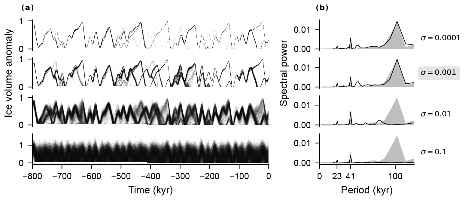
Figure 2 Impact of varying noise levels on stochastic ice volume trajectories and their frequency spectra. (a) 500 stochastic ice volume trajectories for four representative noise levels, $\mathit{\sigma }\in \mathit{\{}\mathrm{0.0001},\mathrm{0.001},\mathrm{0.01},\mathrm{0.1}\mathit{\}}$. The second row highlights the selected value, σ=0.001. (b) Associated ensemble-mean frequency spectra (black line) compared to palaeo data from Spratt and Lisiecki (2016) (grey shading). The x-axis shows period in kyr.

3.1.2 Reference Adherence Ratio (RAR)

To quantify how strongly the simulated ensemble trajectories cluster around the simulated reference path, we introduce the Reference Adherence Ratio, RAR(t). This time-dependent metric measures the fraction of ensemble members that remain within a tolerance band of width α_RAR around the deterministic reference trajectory at each time step:

$$\begin{array}{}\text{(8)}& \mathrm{RAR}\left(t\right)={\displaystyle \frac{\mathrm{1}}{N}}\sum _{k=\mathrm{1}}^N\mathbf{1}\left(\left|{\stackrel{\mathrm{̃}}{v}}_k\left(t\right)-v\left(t\right)\right|<{\mathit{\alpha }}_{\mathrm{RAR}}\right),\end{array}$$

where 1(⋅) is the indicator function, ${\stackrel{\mathrm{̃}}{v}}_k\left(t\right)$ is the ice volume of the kth stochastic realisation, and N is the ensemble size. In our path-resilience framework, a high RAR(t) indicates that a large fraction of perturbed trajectories remains close to the reference path, and is therefore interpreted as higher resilience to stochastic perturbations. Conversely, a low RAR(t) indicates greater divergence from the reference path and is interpreted as lower resilience.

We compute RAR(t) on an ensemble of 1000 stochastic trajectories using α_RAR=0.001, chosen to match the amplitude of the stochastic forcing while remaining sensitive to meaningful deviations.

Figure 3b shows the resulting RAR(t) time series for three representative tolerance values, alongside the unperturbed reference trajectory and stochastic ensemble shown in Fig. 3a. For the main choice α_RAR=0.001, RAR(t) varies substantially over time, typically falling to low values during glacial periods and rising sharply at deglaciations and into interglacials.

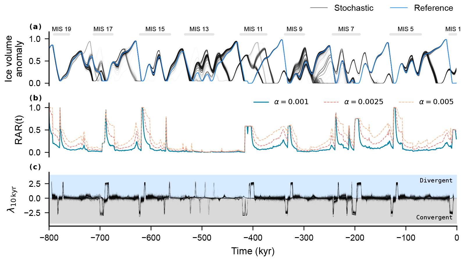
Figure 3 Stochastic ensemble path diagnostics: RAR and finite-time Lyapunov exponent (FTLE). (a) 1000 stochastic ice volume trajectories (black) and the simulated reference (deterministic) trajectory (blue). Interglacial periods are indicated above the panel. (b) RAR(t) computed for three tolerance values, ${\mathit{\alpha }}_{\mathrm{RAR}}\in \mathit{\{}\mathrm{0.001},\mathrm{0.0025},\mathrm{0.005}\mathit{\}}$. The solid curve marks the main choice made in this study, α_RAR=0.001, while the dashed curves show that increasing the tolerance changes the absolute magnitude of RAR(t) but preserves its main temporal pattern. (c) FTLE values λ_10 kyr(k,t) for the same stochastic realisations (black), plotted at the centre of each 10 kyr window. Positive values indicate local divergence over the window and negative values indicate local convergence.

The higher curves obtained for larger α_RAR show the expected increase in absolute adherence when the tolerance band is widened, but the overall timing of peaks and troughs remains similar across all three values. This indicates that the qualitative temporal pattern is not tied to a single threshold choice.

The elevated RAR(t) during interglacials suggests a higher capacity to absorb perturbations. However, this may be partly an artefact of the model's hard constraint that ice volume cannot drop below its pre-industrial value (v≥0). When active, this lower bound prevents downward excursions and can artificially boost RAR(t) by limiting the spread of perturbed trajectories. More indicative of path resilience in our sense are the increases in RAR(t) that occur during the deglaciation phases – periods of rapid ice loss – when the constraint is not yet active and the system is free to evolve. Here the convergence of ensemble members toward the reference trajectory indicates an attracting segment of the forced trajectory, rather than stability of a fixed climate state.

3.1.3 Finite-time Lyapunov exponent

Following Mitsui and Crucifix (2016), we also use a finite-time Lyapunov exponent (FTLE) as a comparison diagnostic for local transient divergence or convergence along the same simulated reference trajectory (Fig. 3). For the deterministic reference trajectory v(t) and the kth stochastic realisation ${\stackrel{\mathrm{̃}}{v}}_k\left(t\right)$, we define the FTLE over a time window of length τ starting at time t as

$$\begin{array}{}\text{(9)}& {\mathit{\lambda }}_{\mathit{\tau }}(k,t)={\displaystyle \frac{\mathrm{1}}{\mathit{\tau }}}\log \left({\displaystyle \frac{\left|{\stackrel{\mathrm{̃}}{v}}_k(t+\mathit{\tau })-v(t+\mathit{\tau })\right|+\mathit{ϵ}}{\left|{\stackrel{\mathrm{̃}}{v}}_k\left(t\right)-v\left(t\right)\right|+\mathit{ϵ}}}\right),\end{array}$$

where $\mathit{ϵ}={\mathrm{10}}^{-\mathrm{14}}$ regularises the ratio when the two trajectories become nearly identical. Positive values indicate local divergence over the chosen window, while negative values indicate local convergence. We use τ=10 kyr (not the memory timescale τ appearing in the ice-volume equation in Sect. 2), because this window is comparable to the timescale of a typical deglaciation and therefore probes transition-scale instability rather than whole-cycle variability.

Panel (c) of Fig. 3 shows the FTLE time series for the same stochastic realisations as in panel (a). The FTLE shows short-horizon intervals of local divergence and convergence that broadly align with the phases identified by RAR(t): deglaciations and interglacials tend to coincide with contraction toward the reference path, while divergence episodes occur more often in glacial phases and shortly after transitions. However, FTLE addresses a different question from RAR(t). It is a local linear diagnostic based on the growth of small separations over a fixed window, whereas RAR(t) measures the fraction of finite perturbations that remain within a prescribed tolerance α_RAR of the reference path under identical forcing.

We therefore retain RAR(t) as the primary path-resilience representation and use FTLE as a complementary comparison with earlier transient-stability studies.

3.2 Experiment II: Pulse-perturbation ensemble and return time

To complement the stochastic ensemble, we also assess the system's resilience to isolated, abrupt perturbations using a pulse-perturbation ensemble. This setup probes the system's ability to recover from discrete shocks applied at specific times along the reference trajectory, rather than from continuous background variability.

At each time step within the simulation window $t\in [-\mathrm{800},-\mathrm{1}]$ kyr, we generate an ensemble of 20 trajectories by applying a one-time perturbation to the ice volume variable, with an amplitude drawn uniformly from the interval $[-\mathrm{0.01},+\mathrm{0.01}]$, resulting in a total of 16 000 perturbed trajectories. The system then evolves deterministically from that point onward. This perturbation amplitude is an order of magnitude larger than the stochastic noise used in the previous experiment (σ=0.001), and is meant to represent more shock-like disturbances.

3.2.1 Return time

We denote the convergence tolerance for sustained return by α_RT, distinct from the adherence band α_RAR used for RAR(t). We define the return time T_R(t_p) as the smallest elapsed time after a perturbation at time t_p for which the perturbed trajectory re-enters a narrow band around the reference trajectory and stays within it for the remainder of the simulation:

$$\begin{array}{}\text{(10)}& T_R\left(t_{\mathrm{p}}\right)=inf\left\{s\ge \mathrm{0}:\forall u\ge s,\left|\stackrel{\mathrm{̃}}{v}(t_{\mathrm{p}}+u)-v(t_{\mathrm{p}}+u)\right|<{\mathit{\alpha }}_{\mathrm{RT}}\right\},\end{array}$$

where t_p is the perturbation time, s and u denote elapsed time after the perturbation, $\stackrel{\mathrm{̃}}{v}$ is the perturbed trajectory, v is the reference trajectory, and α_RT is a strict convergence threshold. We run each trajectory 1000 kyr beyond the perturbation to allow sufficient time for return. If the perturbation does not push the trajectory outside the α_RT-band initially, we assign T_R(t_p)=0.

Return time provides a temporal measure of path resilience, indicating how quickly the system recovers from an isolated shock. Short return times suggest high resilience; long return times indicate prolonged deviation. Conceptually, this aligns with classical engineering resilience metrics (Krakovská et al., 2024) but is applied here to recovery toward a reference trajectory, not a fixed point.

Our return criterion is deliberately strict: unlike exponential decay-based definitions (e.g., $\mathrm{1}/e$ recovery), it requires sustained convergence. This avoids falsely classifying temporary re-approaches as recovery – particularly important in a non-autonomous system where external forcing may later drive re-divergence.

We compute return times using ${\mathit{\alpha }}_{\mathrm{RT}}={\mathrm{10}}^{-\mathrm{6}}$, chosen to ensure persistent re-alignment of perturbed and reference trajectories. Figure 4 presents the results: Fig. 4a shows 16 000 perturbed trajectories (black) alongside the unperturbed reference trajectory, while Fig. 4b displays the distribution of return times for perturbations applied at each time step. The black line shows the median return time, and the shaded region marks the full range across all perturbations.

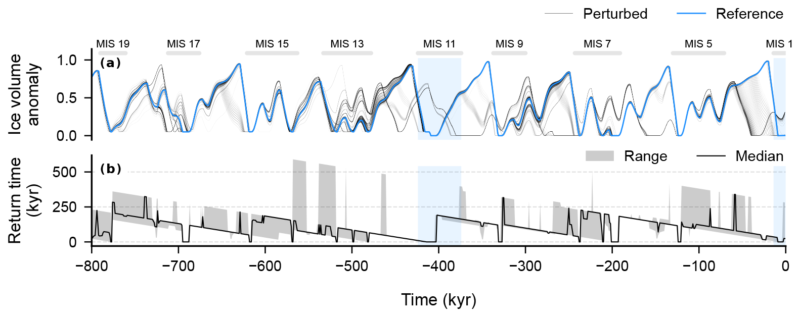
Figure 4 Return time to reference trajectory as a measure of Earth system resilience. (a) Ice volume trajectories from 16 000 pulse perturbations (black) and the unperturbed reference trajectory over the last 800 kyr. Interglacial periods are indicated above the panel. MIS1 (the Holocene) and MIS11, which appear as particularly strong convergence zones in the return-time analysis, are additionally highlighted by light blue shading. (b) Distribution of return times for perturbations applied at each time step. The black line shows the median return time, while the shaded region indicates the full range (minimum to maximum) of return times across all perturbations at each time. Shorter return times correspond to higher resilience. Return time is defined relative to ${\mathit{\alpha }}_{\mathrm{RT}}={\mathrm{10}}^{-\mathrm{6}}$. Each simulation is integrated for 1800 kyr in total, i.e. the 800 kyr analysis window plus an additional 1000 kyr extension.

Return times vary substantially over the glacial-interglacial cycle, generally decreasing as the system approaches interglacial conditions. In particular, MIS11 and the Holocene stand out as strong convergence zones, with many long excursions returning to the reference path. This suggests higher resilience during these periods. One likely explanation is their unusual length: both MIS11 and the Holocene are exceptionally long interglacials due to orbital forcing, providing extended windows for perturbed trajectories to realign (Berger et al., 2016).

Sensitivity tests using larger perturbation amplitudes and more ensemble members (up to 100 per time step) increased the spread of return times but did not change the overall temporal pattern. Likewise, moderately relaxing α_RT shifts absolute return times but preserves the key structure of the results. This confirms that our findings are robust to these parameter choices.

4 Discussion

In this study, we introduced a perturbation-based approach to exploring Earth System resilience, aiming to move beyond traditional attractor-based concepts. By analysing how perturbed trajectories deviate from and return to a reference path, we quantified the system's time-varying resilience over the last 800 kyr of glacial-interglacial dynamics. Our results reveal a strongly state-dependent pattern: during some periods, perturbed trajectories remain tightly clustered around the reference, while during others they diverge widely.

Our stochastic ensemble results align with previous findings by Mitsui and Crucifix (2016), who showed that the timing of stochastic forcing in conceptual climate models can influence the duration and nature of transient excursions. We build on this by explicitly quantifying such detours using resilience metrics, specifically the Reference Adherence Ratio, RAR(t), and return time, and by showing that sensitivity to perturbations depends systematically on the system's position along the glacial cycle. The FTLE comparison in Fig. 3 is broadly consistent with this picture, but it remains a local windowed diagnostic of small-separation growth rather than a direct measure of finite-perturbation recovery.

In particular, MIS11 and the Holocene stand out as strong convergence points where many trajectories recover. Their unusual length and stability, a feature also emphasised in model-based studies of glacial pacing dynamics (Ganopolski, 2024), may explain this exceptional behaviour. More generally, interglacial periods consistently show lower variance in the ensemble, with perturbed trajectories tending to cluster more tightly around the reference path compared to glacial periods, which aligns with palaeoclimate evidence showing that natural temperature variability was lower during interglacial conditions (Rehfeld et al., 2018). Taken together, these findings suggest that path resilience varies systematically across the glacial-interglacial cycle and is often elevated during interglacials and key transition periods, although some of this interglacial signal may reflect structural features of the model. We address these limitations in more detail below.

4.1 Model limitations

Several limitations of the model should be kept in mind when interpreting the results. Most importantly, the apparent resilience during interglacials may partly be an artefact of a hard lower bound imposed on ice volume (v≥0), which prevents trajectories from falling below pre-industrial levels. This constraint leads to extended periods of zero ice volume and artificially suppresses variability during interglacials, potentially inflating both RAR(t) and the apparent tendency toward shorter return times. Future work should compare results across models without such constraints to assess the extent of this effect.

A further limitation lies in the model's non-Markovian structure. It includes a memory term that integrates ice volume over the past 30 kyr, making it effectively infinite-dimensional and preventing the use of standard Jacobian-based stability analysis. This justifies our simulation-based approach, but also limits direct comparisons with studies that rely on linearised stability frameworks.

The present indicators should also be interpreted as simple illustrative diagnostics rather than universal resilience measures. Their role here is to demonstrate a path-resilience perspective in a controlled conceptual model, not to provide directly transferable tools for arbitrary systems or datasets. Relatedly, the tolerances α_RAR (for RAR(t)) and α_RT (for return time) should be viewed as proof-of-concept, model-specific choices. Future work could instead scale such thresholds relative to quantities such as the range, variance, or other characteristic amplitudes of the time series under study.

Another limitation is that our analysis assumes a single deterministic reference trajectory for a fixed parameter set. In systems with multiple coexisting deterministic trajectories, stronger initial-condition dependence, or chaotic but partially synchronised responses to forcing, the definition of a single reference path becomes less straightforward. In such cases one could define the reference trajectory conditionally on a chosen initial condition, or use an unperturbed ensemble mean or median together with an ensemble-based spread measure.

Finally, the model lacks self-sustained oscillations, which have been proposed as key ingredients in explaining the 100 000-year glacial pacing problem (Ganopolski, 2024). Our results therefore reflect the resilience of a purely forced system and may change in models that include internally driven oscillations. A natural next step is to validate the findings with a more complex model, but given the need for large ensembles, there are computational challenges. It may be possible using Earth system models of intermediate complexity like CLIMBER-X, which can simulate 10,000 simulation years per day on a node with 16 CPUs (Willeit et al., 2022, 2023). If run on a more powerful cluster, one could generate a single 1 million year simulation in around 20 d, but it becomes clear that large ensembles are limited. Fully integrated Earth system models would require computational resources that make comparable ensemble experiments currently impractical.

Despite these limitations, our approach connects to a broader shift in how resilience is conceptualised and operationalised in non-autonomous systems, as discussed next.

4.2 Relationship to existing research

Classical resilience indicators are designed for autonomous systems near equilibrium, where concepts like basins of attraction and return time to fixed points are well-defined. Several studies have highlighted the lack of tools for analysing resilience in forced, transient systems (Krakovská et al., 2024). Our approach addresses this gap by using ensemble perturbations to evaluate system stability over time, offering a first step toward quantifying resilience in non-autonomous systems.

We see this work as a practical example of path resilience thinking, applied to palaeoclimate dynamics. The concept of path resilience (Anderies et al., 2023) shifts the focus from return to equilibrium states to return to a reference trajectory – making it more appropriate for externally forced systems like the glacial-interglacial cycle.

This perspective complements, rather than replaces, several existing approaches. In studies of conceptual glacial-cycle models, finite-time Lyapunov exponents have been used to identify intervals of transient divergence and local instability of nearby trajectories (De Saedeleer et al., 2013; Mitsui and Crucifix, 2016). Potential analysis has been used to infer changes in effective climate states and basin structure from palaeoclimate time series (Livina et al., 2011), while early-warning-signal methods have sought signs of critical slowing down before abrupt climate transitions (Dakos et al., 2008). Our FTLE comparison in Fig. 3 follows this line of work and confirms that short-horizon local divergence and convergence vary strongly along the glacial cycle. There, FTLE (λ) and RAR(t) align in phase: convergent λ often precedes rising RAR(t), divergent λ when spreads widen – expected, since both follow the same path but FTLE uses local separation growth over the 10 kyr window while RAR(t) is the within-tolerance fraction.

Related work by Medeiros et al. (2023) uses time-varying Jacobians and eigenvectors to assess sensitivity in ecological communities. While powerful, their method assumes differentiable, Markovian dynamics. In contrast, our model includes a memory term – an integral over past ice volume – which makes standard Jacobian-based methods inapplicable. This motivates our use of a model-agnostic, simulation-based strategy that can handle non-Markovian dynamics.

Our approach builds on Hasselmann's programme for stochastic climate modelling (Hasselmann, 1976), where unresolved processes are treated as noise. This perspective laid the foundation for analysing climate variability through probabilistic ensemble dynamics and has recently been extended by Lucarini and Chekroun (2023) and others through operator-theoretic methods. In particular, transfer operator theory provides a systematic framework for describing the evolution of probability distributions in phase space and has been used to study mixing, regime transitions, and responses in high-dimensional systems. These methods offer conceptual and computational tools that could support more general resilience indicators – especially in systems with complex dynamics and non-equilibrium behaviour.

However, while transfer operator methods are well developed for autonomous, Markovian systems, they are not yet fully applicable to systems with memory (non-Markovian dynamics), and a general theoretical framework for analysing stability and resilience in non-autonomous systems – such as those driven by orbital forcing – remains underdeveloped (Froyland et al., 2010; Lucarini and Chekroun, 2023).

5 Conclusion

As humanity continues to push the Earth system toward new and potentially unstable modes of operation, understanding the resilience of both past and projected trajectories becomes increasingly critical. The approach developed here represents a step toward that goal by enabling resilience analysis in externally forced, non-autonomous systems that do not settle into traditional equilibrium states.

We introduced a simulation-based method to assess path-based Earth system resilience across glacial-interglacial cycles. By applying perturbations to a reduced-complexity climate model and analysing trajectory responses, we show that resilience varies markedly over time and depends on the system's state at the moment of disturbance.

Our findings reveal that resilience fluctuates throughout the glacial-interglacial cycle, reflecting the evolving dynamical landscape of the system. Interglacial periods – particularly MIS11 and the Holocene – consistently draw perturbed trajectories back toward the reference path, suggesting enhanced recovery capacity linked to their unusual duration. Deglaciation phases show similar behaviour, with trajectories reconverging even before interglacial conditions are reached. The Reference Adherence Ratio and return time provide useful, albeit preliminary and deliberately simple, indicators of resilience in non-autonomous systems, while the finite-time Lyapunov exponent offers a complementary comparison diagnostic for local transient divergence.

These results mark an initial proof of concept for quantifying resilience in settings where traditional equilibrium-based tools fall short. The path-resilience framework shifts focus from fixed-point attractors to the stability of entire trajectories – an essential perspective for assessing the resilience of transient climate states as the Earth system moves into uncharted territory under anthropogenic forcing (Summerhayes et al., 2024).

Several limitations must be acknowledged. The model's hard lower bound on ice volume may inflate apparent resilience during interglacials, and its non-Markovian structure prevents standard stability analysis. Moreover, the model lacks self-sustained oscillations that could influence glacial pacing. Despite these simplifications, the study demonstrates the potential of trajectory-based resilience assessment in externally forced systems.

Future work should test and extend this framework across other conceptual and intermediate-complexity models such as CLIMBER-X (Willeit et al., 2022, 2023) and LOVECLIM (Goosse et al., 2010). Developing more advanced resilience indicators for non-autonomous dynamics remains a key priority – promising directions include transfer operator theory, pullback attractors, and random dynamical systems.

This line of research aligns with Hasselmann's view of the climate as a stochastically forced dynamical system. Recent work by Lucarini and colleagues (Lucarini and Chekroun, 2023) has begun to formalise this perspective, paving the way for robust, operator-based resilience metrics. Advancing these ideas could deepen our understanding of Earth system resilience and support the development of general tools for resilience assessment.

Appendix A: Model calibration via Metropolis-Hastings MCMC

To recalibrate the model described by Talento and Ganopolski (2021), a Metropolis-Hastings Markov Chain Monte Carlo (MCMC) algorithm (Hastings, 1970) was implemented, targeting agreement between simulated and reconstructed ice volume anomalies over the past 800 kyr based on the sea-level stack from Spratt and Lisiecki (2016). The recalibration achieved a Pearson correlation coefficient of 0.892.

The algorithm proceeds as follows:

1. An initial model run m(p) is generated using the published parameter set p from Talento and Ganopolski (2021), as shown in Table A1.

2. One parameter p_i is randomly selected and perturbed by a small factor drawn from a normal distribution 𝒩(1,σ) with σ=0.05:

   $$\begin{array}{}\text{(A1)}& {\widehat{p}}_i=\mathcal{N}(\mathrm{1},\mathrm{0.05})\cdot p_i,\end{array}$$

   resulting in a new candidate parameter set $\widehat{\mathit{p}}$.

3. A model run $\widehat{\mathit{m}}\left(\widehat{\mathit{p}}\right)$ is performed using the perturbed parameters, and the likelihood of the resulting ice volume time series is computed as:

   $$\begin{array}{}\text{(A2)}& L=-\sum _{t=\mathrm{1}}^{t_{\mathrm{end}}}{\left[v_{\mathrm{model}}\left(t\right)-v_{\mathrm{palaeo}}\left(t\right)\right]}^{\mathrm{2}}-P_{\mathrm{LGM}}-P_{{\mathrm{CO}}_{\mathrm{2}}},\end{array}$$

   where P_LGM penalises poor agreement with the Last Glacial Maximum:

   $$\begin{array}{}\text{(A3)}& P_{\mathrm{LGM}}=\mathit{\alpha }{\left[\mathrm{1}-v\left(t_{\mathrm{LGM}}\right)\right]}^{\mathrm{2}}\text{with}\mathit{\alpha }=\mathrm{1000},\end{array}$$

   and $P_{{\mathrm{CO}}_{\mathrm{2}}}$ discourages solutions with unrealistically high CO₂ concentrations:

   $$\begin{array}{}\text{(A4)}& P_{{\mathrm{CO}}_{\mathrm{2}}}=\sum _{t=\mathrm{1}}^{t_{\mathrm{end}}}{\left(max\left[\mathrm{0},{\mathrm{CO}}_{\mathrm{2}}\left(t\right)-\mathrm{300}\right]\right)}^{\mathrm{2}}.\end{array}$$

4. The perturbed model is accepted with probability:

   $$\begin{array}{}\text{(A5)}& p_{\mathrm{accept}}=min\left(\mathrm{1},\exp (\widehat{L}-L)\right),\end{array}$$

   where $\widehat{L}$ is the likelihood of the candidate model. Otherwise, the previous model is retained.

5. Steps 2–4 are repeated for N=5000 iterations per chain.

To ensure robustness, the procedure was repeated for 1000 independent chains, each with a different random seed. The best-fitting model across all runs achieved a maximum correlation of 0.892, with the corresponding parameter values listed in Table A1. These calibrated parameters were used for all simulations in this study unless stated otherwise.

Table A1 Unrounded model parameters from Talento and Ganopolski (2021) and from the Metropolis-Hastings MCMC recalibration performed in this study. These parameters were used for all simulations unless stated otherwise.