Global hyper-resolution modeling of historical and future groundwater dynamics

The sustainable management of global groundwater resources is a key societal challenge and is central to the Sustainable Development Goals. The localized dynamics of groundwater abstraction, topography, and surface-water interactions, as well as the sensitivity of groundwater-dependent ecosystems, call for high-resolution information to support effective groundwater management. At the same time, groundwater observations are very limited and concentrated in a few regions, rendering large parts of groundwater resources ungauged. To address limited observations and coarse global models, we applied the global groundwater model GLOBGM (v1.1) to simulate past and future groundwater heads and water table depth at 30 arcsec (∼ 1 km) on a monthly time step. Model calibration improved mean bias in water table depth predictions from −4.8 to 3.6 m compared to GLOBGM v1.0, with depth-weighted bias reduced from 34.2 to 32.5 m across 34 800 observation wells. Groundwater dynamics are simulated for a historical reference period (1960–2019) to support model evaluation and attribution of observed impacts to climate variability and change. Baselines (1960–2014) and three combined socioeconomic-climate scenarios (2015–2100; SSP1-RCP2.6, SSP3-RCP7.0, SSP5-RCP8.5) are simulated with five global climate models, supporting detection and impact assessment of future change. Validation against monthly observations yielded skillful predictions (KGE-NP_skill) in approximately 60 % of deep wells (> 60 m) and 83 % of shallow to intermediate wells (0–60 m). When validated against annual observations, 66 % of deep wells (> 60 m) and 71 % of shallow to intermediate wells (0–60 m) were skillful. Simulations are further bias corrected using a machine learning approach. Historical trend analysis (1960–2019) accurately reproduced known groundwater depletion regions such as the U.S. High Plains, Arabian Peninsula, and Indo-Gangetic Plain, while also identifying rising water tables in northern latitudes and Arctic regions, which are linked to climate-driven recharge changes. Future scenario-based simulations suggest rising water tables for most continents in the next century, with Europe being a notable exception. However, known regions of groundwater depletion are expected to persist. Regions that disagree with observations or show reduced reliability are mapped, and quality assurance flags are provided to guide the appropriate use and interpretation of the results. The resulting data set offers high-resolution information to assess groundwater dynamics for the past and future, supporting improved global water resource management and climate impact assessments.

1 Introduction

Groundwater is the most abundant source of fresh liquid water; globally, 98 % of accessible fresh liquid water is in the form of groundwater (Döll et al., 2012; Gleeson et al., 2020). People increasingly rely on these resources to supplement surface water abstractions to meet total water demands (Custodio, 2010). Groundwater is vulnerable to overexploitation when abstraction rates persistently exceed natural groundwater recharge – the process by which surface water and precipitation infiltrate the soil to replenish aquifers. Driven by population growth and associated increases in water demand for agriculture, domestic, and industrial purposes, groundwater abstraction has increased significantly in recent decades, ultimately causing a decline in groundwater storage in many regions (Bierkens and Wada, 2019; Niazi et al., 2024; Wada and Bierkens, 2014; Kuang et al., 2024; Rodell et al., 2018; Döll et al., 2012; Leijnse et al., 2024). Besides anthropogenic pressures, groundwater is sensitive to decadal and annual climate variability and its influence on groundwater recharge (Taylor et al., 2013; Moeck et al., 2020b). These effects are complex, vary geographically, and are mediated by interactions between topography, vegetation, underlying geological properties, and surface water-groundwater exchange (Moeck et al., 2020b; Maples et al., 2019). For example, groundwater in deep confined aquifers with low permeability is relatively insensitive to changes in short-term recharge dynamics, whereas groundwater in highly permeable shallow aquifers with vegetation that facilitates exchanges across the land-atmosphere continuum is more tightly coupled to recharge variability (Ilstedt et al., 2016; West et al., 2022; Maples et al., 2019). Consequently, the future of groundwater storage depends on complex interactions among human water demands, climate, and ecosystems (Vörösmarty et al., 2000; Wada and Bierkens, 2014).

Overexploitation of groundwater causes water table depths to decline, a consequence of groundwater abstraction evident in many regions, especially in arid and dryland areas (Jasechko and Perrone, 2021; Jasechko et al., 2024). This reduces groundwater's reliability as a water source, given the physical and economic constraints associated with abstracting deeper reserves (Perrone and Jasechko, 2019). Since half of global river flows are groundwater-sustained, deepening water tables threaten downstream surface water supplies (de Graaf et al., 2024; Xie et al., 2024; Bierkens et al., 2021) and may increase vulnerability to hydrological drought (Wada et al., 2013; Vega-Briones et al., 2024). Reduced reserves also cause land subsidence, accelerate sea level rise, and degrade groundwater quality (Kuang et al., 2024; Bierkens and Wada, 2019). Deeper water table depths also influence the composition and functioning of groundwater-dependent ecosystems and the services they provide (Saccò et al., 2024; Fan et al., 2017; Otoo et al., 2025). Ultimately, groundwater forms an important component of global socio-ecological systems and the Earth system as a whole (Huggins et al., 2023).

Sustainable management of the world's remaining groundwater reserves is a key societal challenge and is cited in several Sustainable Development Goals (Garrick et al., 2017; UN Water, 2022). Policymakers must implement adaptation and mitigation strategies to secure water availability by maintaining groundwater levels within safe operating limits. However, this requires reliable estimates of current and future groundwater volumes. Relying solely on observed groundwater data is insufficient given the severe limitations in global spatial and temporal coverage (Condon et al., 2021; UN Water, 2022). For example, the current state-of-the-art dataset contains 180 000 groundwater time series from 41 countries, with over 90 % of these time series occurring in North America, Australia, or Europe (Bäthge et al., 2026). To overcome this challenge and provide global-scale information, water managers rely on physically based numerical global groundwater models (Condon et al., 2021). However, until now, most groundwater flow models have had limited spatial extent, allowing regional-scale analyses (≤ 1 000 000 km²) at most (Zamrsky et al., 2025).

Groundwater models of global extent were first formulated in the past decade (Fan et al., 2013), with more recent efforts enabling transient simulations (Reinecke et al., 2019; Costantini et al., 2023; de Graaf et al., 2019). However, these models provide information at spatial resolutions that are often too coarse to meet the demands of policymakers and stakeholders, who require finer-scaled information (Condon et al., 2021; Bierkens et al., 2015). To overcome this limitation, spatial resolution must be enhanced to make global models more locally relevant and actionable (Bierkens et al., 2015; Wood et al., 2011). To this end, hyper-resolution groundwater models have been highlighted for their potential to include climate, vegetation, and anthropogenic influences on groundwater at appropriate spatial resolutions for past and future (Bierkens et al., 2015). This is especially relevant, as hyper-resolution models can define current water scarcity hotspots, project future hotspots, and support the planning of adaptation strategies (Leijnse et al., 2024; Bierkens, 2015). Recent work demonstrates that global groundwater models at ∼ 1 km spatial resolution are possible with today's high performance computers (Verkaik et al., 2024; Kollet et al., 2026). This technical development offers the opportunity to generate global hyper-resolution estimates of past and future groundwater reserves at scales relevant to policymakers.

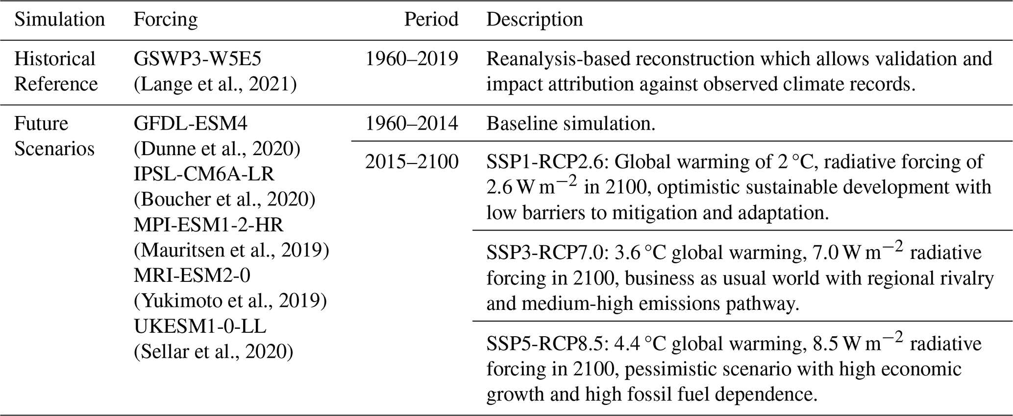
This study aims to produce the first hyper-resolution monthly estimates of global groundwater storage, incorporating the impacts of climate change and human activities across past and future periods. To this end, using scenarios and global climate models (GCMs) from the Inter-Sectoral Impact Model Intercomparison Project (ISIMIP), monthly groundwater heads and water table depths are simulated at 30 arcsec (∼ 1 km at the equator). We use the ISIMIP3a climate forcing to simulate groundwater reserves for the historical reference period (1960–2019), which can be used for detection and attribution of past climate and socioeconomic change impacts on groundwater reserves. To project future trends, we employ ISIMIP3b inputs from a suite of five GCMs, covering both the baseline (1960–2014) and future periods (2015–2100) under combined socioeconomic and climate change scenarios (SSP1-RCP2.6, SSP3-RCP7.0, and SSP5-RCP8.5). These simulations are analyzed by calculating long-term trends, providing a global initial assessment of historical shifts in the global groundwater system and how it may change in the future.

2 Methods

2.1 The GLOBGM v1.1 model

Monthly estimates of groundwater heads and water table depths were simulated using GLOBGM v1.1, a global 30 arcsec, two-layer transient, MODFLOW-based groundwater flow model. GLOBGM is the successor to the 5 arcmin version originally developed by de Graaf et al. (2017). For brevity, we refer to Verkaik et al. (2024) for a detailed description of model inputs, parametrization, and runtime configurations. Briefly, GLOBGM is based on a prototype version of MODFLOW6, which is parallelized using message-passing interface and makes use of unstructured grids. Independent unstructured grids are distributed over three continental-scale groundwater models – Afro-Eurasia, the Americas, Australia – and one remaining model for the islands (Fig. 1). Each of the four groundwater models is partitioned into non-overlapping sub-models that are coupled within the MODFLOW linear solver. The two-layer configuration represents unconfined, confining, or confined aquifer systems (Verkaik et al., 2024). For cells where a confining layer is present, the top model layer represents the confining layer, and the bottom layer is the confined aquifer; in regions where a confining layer is absent, the bottom model layer represents the unconfined aquifer. GLOBGM employs an offline coupling approach whereby 5 arcmin resolution local runoff, groundwater abstraction, and groundwater recharge from PCR-GLOBWB2 (Sutanudjaja et al., 2018) are resampled to match GLOBGM's 30 arcsec grid.

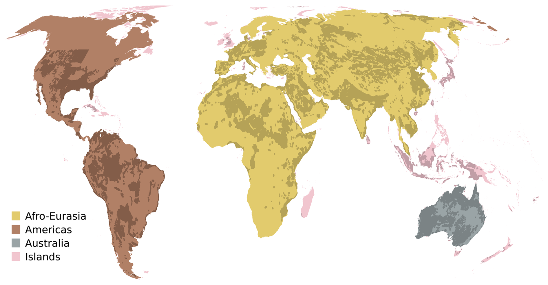
Figure 1 The four groundwater models that constitute GLOBGM, a global groundwater model. Dark overlays indicate the presence of a confining layer.

GLOBGM v1.1 builds upon GLOBGM v1.0 (Verkaik et al., 2024), and in contrast to GLOBGM v1.0, a dynamic drainage elevation routine was implemented to better represent permanent wetland areas and groundwater-surface water exchange. To address a major source of uncertainty in global modeling, the updated version also incorporates a new downscaling method for groundwater recharge using observed data (Reinecke et al., 2024; Gnann et al., 2023; Bierkens and Wada, 2019). The treatment of river discharge and abstraction is consistent with GLOBGM v1.0. River discharge from PCR-GLOBWB2 was converted to 30 arcsec by accumulating it through the 30 arcsec HydroSHEDS river drainage network (Lehner et al., 2008; Verkaik et al., 2024), which is then converted to surface water levels using Manning's equation. The 30 arcsec surface water levels thus obtained were subsequently used to parameterize the MODFLOW river and drainage boundary conditions; GLOBGM then computes groundwater-river exchange as a head-dependent flux based on simulated heads, stage, and conductance. Groundwater abstraction was resampled to 30 arcsec using a nearest neighbor algorithm.

2.1.1 Dynamic Drainage Elevation

In the dynamic drainage elevation routine, each cell's drain elevation adjusts based on soil saturation. As soils become wetter, the drainage elevation rises closer to the surface; as they dry, it lowers toward the base elevation. Discharge occurs only when the hydraulic head exceeds this dynamic drain level (Eq. 1). By coupling drain elevation to saturated area fractions, this approach maintains groundwater levels closer to the surface in wetland areas, thereby reducing unrealistic head fluctuations and highly intermittent discharge events. To simulate variations in the saturated area fraction, the improved ARNO scheme (Todini, 1996; Hagemann and Gates, 2003), an integral part of PCR-GLOBWB2, identifies areas subject to surface runoff.

$$\begin{array}{}\text{(1)}& f_{\mathrm{sat}}=\mathrm{1}-{\left({\displaystyle \frac{W_{max}-W}{W_{max}-W_{min}}}\right)}^{\frac{\mathit{\beta }}{\mathit{\beta }+\mathrm{1}}}\end{array}$$

where W_max is the maximum water storage, W_min is the minimum water storage, W is the actual water storage, and β is a dimensionless shape parameter in PCR-GLOBWB2.

2.1.2 Groundwater Recharge Downscaling

Accurately predicting groundwater recharge remains a challenge for current global hydrological models (Reinecke et al., 2024; Gnann et al., 2023; Bierkens and Wada, 2019). Previous studies have shown that PCR-GLOBWB2, to which GLOBGM is coupled, tends to underestimate recharge rates compared with observations (Berghuijs et al., 2024). The bias is most pronounced in arid or semi-arid regions where recharge rates are low, intermittent, and unpredictable (Berghuijs et al., 2024). Furthermore, GLOBGM v1.0 predicts groundwater heads that are generally lower than in situ observations and other large-scale groundwater models (Reinecke et al., 2024; Verkaik et al., 2024). To address these challenges, recharge supplied to GLOBGM v1.1 was downscaled and corrected using observed groundwater recharge data.

Moeck et al. (2020a)Zamrsky et al. (2024)Poggio et al. (2021)Brun et al. (2022b)Verkaik et al. (2024)Sutanudjaja (2024)

Table 1 Response and predictor variables used for groundwater recharge downscaling.

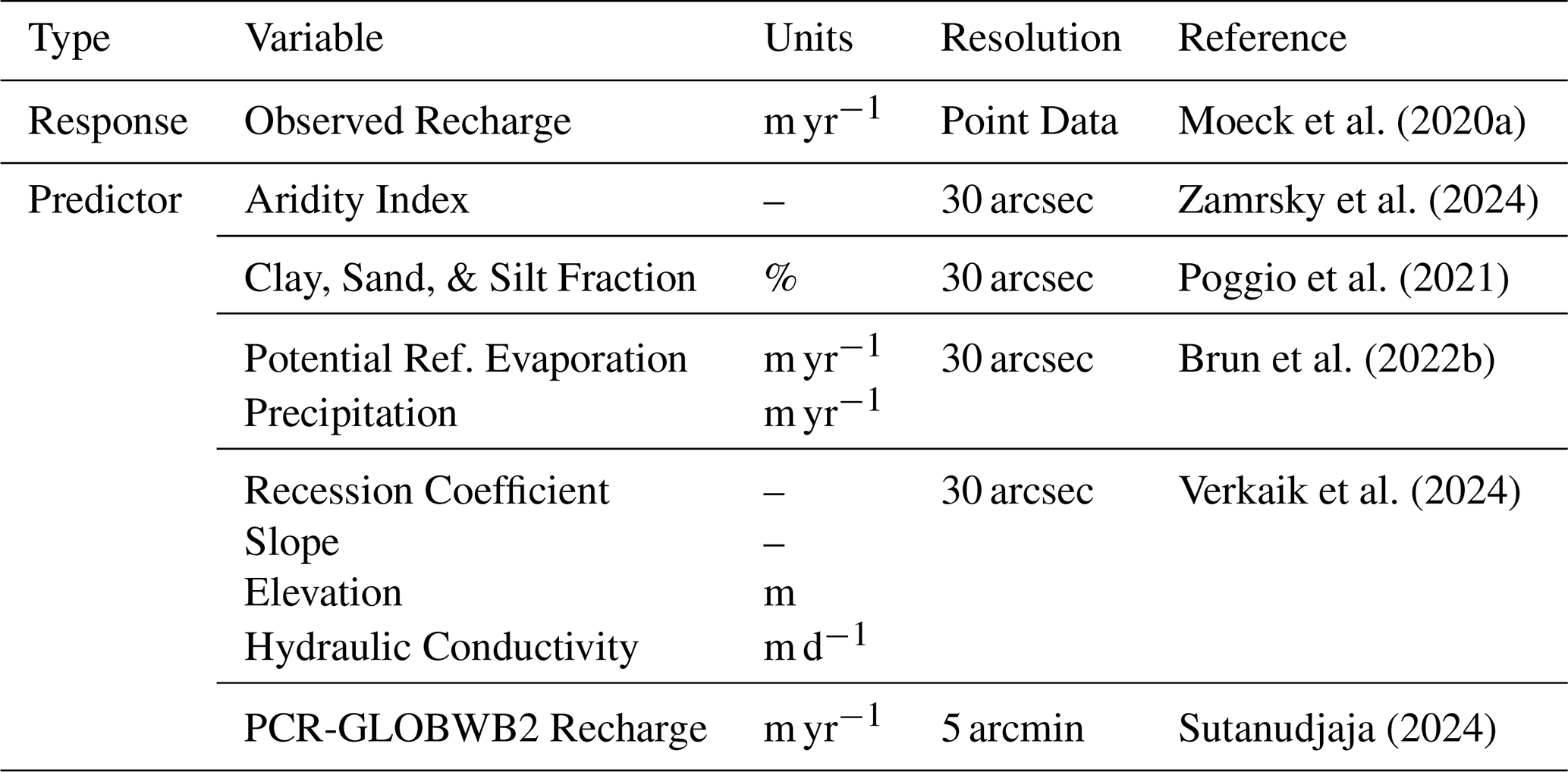
A Generalized Additive regression approach using pyGAM (Servén et al., 2018) was employed to produce a long-term average 30 arcsec recharge field (GWR_observed) from known drivers and covariates (Table 1). This approach has previously been applied in groundwater modeling contexts (Mohan et al., 2018; Zamrsky et al., 2025). In contrast to these studies, land cover was not explicitly included as a predictor here; instead, the 5 arcmin PCR-GLOBWB2 recharge was included to capture land cover-associated residuals by proxy. In Appendix A, we elaborate on the performance of the pyGAM model in predicting recharge. To prevent unrealistic recharge rates, GWR_observed was further processed to ensure it did not exceed local precipitation rates (Brun et al., 2022a, b). Finally, to calculate a correction factor (GWR_cf), GWR_observed was compared with PCR-GLOBWB2 5 arcmin recharge (bilinearly interpolated to 30 arcsec) from a GSWP3-W5E5 forced naturalized run (Eq. 2). For the steady-state simulation, the 5 arcmin PCR-GLOBWB2 recharge was interpolated to the 30 arcsec GLOBGM v1.1 grid via bicubic interpolation and corrected (Eq. 3). For the transient simulations, for each time step, PCR-GLOBWB2 was interpolated and corrected (Eq. 3) and, to avoid unrealistic estimates, recharge values were constrained by local precipitation rates (Eq. 4).

$$\begin{array}{}\text{(2)}& {\mathrm{GWR}}_{\mathrm{cf}}={\displaystyle \frac{{\mathrm{GWR}}_{\mathrm{observed}}}{{\mathrm{GWR}}_{\mathrm{5}{\mathrm{arc}}^{\prime }}}}\end{array}$$

where GWR_observed is the observed recharge field and ${\mathrm{GWR}}_{\mathrm{5}{\mathrm{arc}}^{\prime }}$ is the 5 arcmin recharge from PCR-GLOBWB2 interpolated to 30 arcsec.

$$\begin{array}{}\text{(3)}& {\mathrm{GWR}}_{\mathrm{corrected}}={\mathrm{GWR}}_{\mathrm{5}{\mathrm{arc}}^{\prime }}\times {\mathrm{GWR}}_{\mathrm{cf}}\end{array}$$

where GWR_cf is the correction field and ${\mathrm{GWR}}_{\mathrm{5}{\mathrm{arc}}^{\prime }}$ is the 5 arcmin recharge from PCR-GLOBWB2 interpolated to 30 arcsec.

$$\begin{array}{}\text{(4)}& \begin{array}{rl}& {\mathrm{GWR}}_{\mathrm{corrected}}=\\ & \left\{\begin{array}{ll}{P}_{\mathrm{month}}& \text{if }{\mathrm{GWR}}_{\mathrm{corrected}}>P_{\mathrm{month}}\\ {\mathrm{GWR}}_{\mathrm{corrected}}& \text{if }{\mathrm{GWR}}_{\mathrm{corrected}}\le P_{\mathrm{month}}\end{array}\right.\end{array}\end{array}$$

where GWR_corrected is the corrected recharge field and P_month is the local precipitation for the month.

A multiplicative correction factor was chosen to avoid negative recharge values. The multiplicative correction factor, fitted on long-term mean recharge estimates, produced unrealistically high recharge rates when applied directly at the monthly time step during the transient simulation, particularly during wet months. To prevent the numerical instabilities and convergence failures that arose from these excessive fluxes, an upper bound was imposed on the corrected monthly recharge. Monthly precipitation was selected as this constraint, implicitly assuming that precipitation excess can be transferred to recharge within a single monthly time step. This assumption holds in many climatic settings but is conservative in arid environments, where dry-month precipitation is negligible and the correction is suppressed. An annual precipitation bound would relax this suppression in dry months, but permit monthly recharge fluxes that exceed physically plausible rates which would redistribute recharge in time rather than correcting it. We chose the monthly constraint to preserve numerical stability and plausible monthly fluxes, at the cost of dry-month recharge in water-limited regions.

2.2 Calibration, spin-up and initial conditions

GLOBGM v1.0 was uncalibrated, and initial conditions were calculated using a method inherited from its predecessor, PCR-GLOBWB2 (Verkaik et al., 2024; de Graaf et al., 2019). This process involved simulating steady-state groundwater heads under naturalized conditions, followed by a transient spin-up period in which the first year of forcing was repeated back-to-back. However, uncalibrated models prove less accurate than calibrated counterparts, such as the CONUS groundwater and global-scale inverse models (Verkaik et al., 2024; Zell and Sanford, 2020; Fan et al., 2013). Furthermore, spurious trends were evident in GLOBGM v1.0 simulations (Verkaik et al., 2024). To address these limitations, GLOBGM v1.1 presented here was calibrated, and an alternative spin-up procedure was implemented.

2.2.1 Calibration

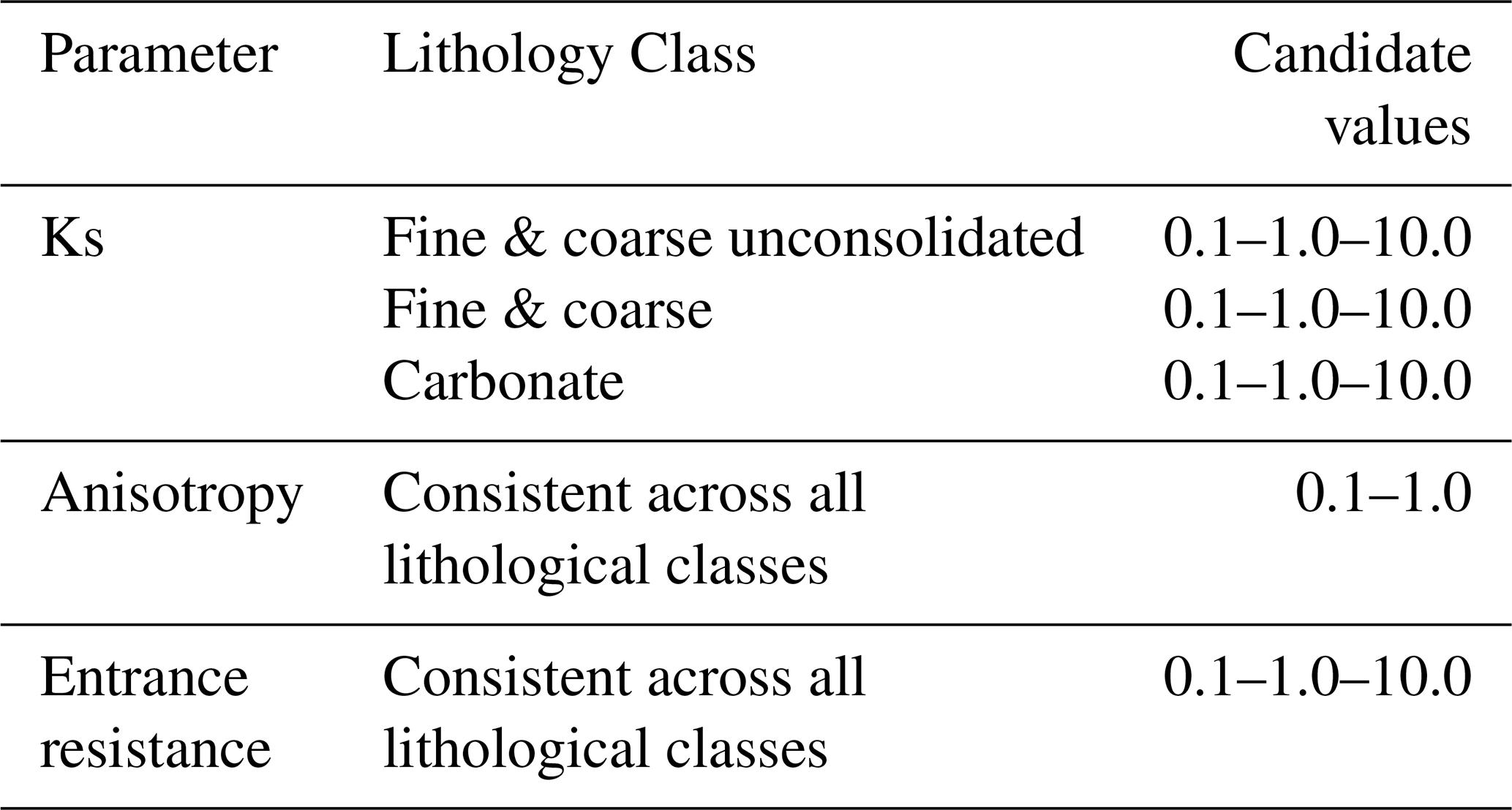
To improve the accuracy of groundwater heads and water table depths simulated by GLOBGM v1.1, hydraulic conductivity, anisotropy, and entrance resistance parameters were calibrated using the steady-state solution. For anisotropy and entrance resistance, a range of global prefactor adjustments was assessed (Table 2). While a broader range of prefactors was possible, adjustments were limited to within two orders of magnitude. This constraint prevented significant departures from the original model parameterization, which was necessary given the spatially concentrated distribution of observations. Previous calibration attempts on the 5 arcmin predecessor reported limited sensitivity to variations in hydraulic conductivity when applied as a global prefactor to the entire domain (Otoo et al., 2025). Therefore, to incorporate regional sensitivities to changes in hydraulic conductivity, different combinations of prefactors were assessed (Table 2), which varied by lithological class (Hartmann and Moosdorf, 2012). In total, 162 permutations were assessed.

Table 2 Parameters and prefactors used during calibration. Lithologies are from the GLiM dataset (Hartmann and Moosdorf, 2012).

Candidate calibration values were assessed by running the steady-state solution for the historical reference simulation (Sect. 2.3) under pristine natural conditions (i.e., unaltered by anthropogenic influence on surface water and groundwater dynamics). Note that updates regarding groundwater recharge downscaling and saturated area fraction adjustments were included prior to calibration (Sect. 2.1.1 & 2.1.2). To select optimal calibration settings, long-term averaged groundwater table depths from observations that overlapped with the forcing period (i.e., 1960–2019) were used, obtained from IGRAC's Global Groundwater Monitoring Network (IGRAC, 2024). Given that the steady-state solution of GLOBGM v1.1 was forced with data representative of the hydrological cycle in a pristine state, observations were filtered to exclude regions with substantial groundwater abstraction. Specifically, observations were filtered to exclude known hotspots for water scarcity (Leijnse et al., 2024), as these regions likely experience extensive groundwater abstraction. Including observations from groundwater abstraction hotspots would confound the effects of groundwater abstraction with model error and skew calibration toward correcting for depletion. Using the filtered dataset of 34 800 observation wells, calibration permutations were evaluated by the mean bias over all locations (Bias_WTD; Eq. 5).

$$\begin{array}{}\text{(5)}& {\mathrm{Bias}}_{\mathrm{WTD}}={\mathrm{WTD}}_{\mathrm{obs}}-{\mathrm{WTD}}_{\mathrm{sim}}\end{array}$$

where WTD_sim is the simulated water table depth and WTD_obs is the observed water table depths.

To enable a direct comparison between model simulations and observations, we used the water table depth outputs from GLOBGM v1.1, derived from heads and surface elevation. Note that due to this conversion and Eq. (5), a positive bias indicates that simulated water table depths are shallower than observed, whereas a negative bias indicates that they are deeper. For unconfined aquifers, where no confining layer is present, observations were assigned to the bottom model layer. Where a confining layer was present in the model, observations were assigned to the correct model layer based on the reported filter. If filter depth was not reported, model layers were assigned using an approach that evaluates the correlation between remotely sensed soil moisture data and simulated groundwater heads, as done by Verkaik et al. (2024). More specifically, if the observed groundwater time series, when expressed as groundwater heads, correlated well (> 0.5) with soil moisture (ESA CCI SM; Dorigo et al., 2017), it was assigned to the upper model layer (i.e., confining layer); if no correlation was found, it was assigned to the bottom model layer (i.e., confined aquifer).

We selected the optimal calibration set by prioritizing the accuracy of shallower estimates (< 60 m), as these reserves are more relevant for human use and for sustaining ecosystems through baseflow contributions to surface water bodies and groundwater-dependent ecosystems (de Graaf et al., 2019; Reinecke et al., 2024; Fan et al., 2013). Mean absolute bias per depth class (< 0, 0–5, 5–10, 10–20, 20–60, > 60 m) was calculated. The mean of the per-class absolute bias values was used as the overall performance score for each permutation. Calibration permutations were rank ordered by average depth weighted absolute bias, and the top ten were identified.

2.2.2 Spin-up and initial conditions

We aimed to derive a set of initial groundwater head states for the simulation start year (i.e., 1960), such that initial conditions resemble the observed data available for 1960. First, the steady-state estimates of groundwater heads under pristine natural conditions were obtained. These steady-state results served as the starting point for a transient simulation for the year 1960, without abstraction, for 75 iterations back-to-back. Subsequently, a second transient simulation for the year 1960, with abstraction activated, was conducted for 50 iterations, allowing simulated groundwater levels to approach observed levels. For this spin-up protocol, GLOBGM v1.1 was forced with data relevant to the historical reference simulation described in Sect. 2.3. Similar to the calibration methodology, observed water table depth data were obtained from IGRAC's Global Groundwater Monitoring Network. Observations were filtered for the year 1960 (375 observation wells). At the end of each iteration, Bias_WTD (Eq. 5) and percentage bias (PBIAS, Eq. 6) were calculated. Simulated and observed water table depths were assigned to the correct model layer as done in Sect. 2.2.1. Our goal was to minimize the difference between modeled and observed groundwater depths of the starting year (i.e., 1960), using the convergence of Bias_WTD and PBIAS as indicators of stability. To assess the evolution of head estimates over the model domain, the average groundwater head for each sub-model was calculated ($\stackrel{\mathrm{‾}}{\mathrm{HDS}}$; Eq. 7).

$$\begin{array}{}\text{(6)}& {\mathrm{PBIAS}}_{\mathrm{WTD}}={\displaystyle \frac{\sum ({\mathrm{WTD}}_{\mathrm{sim}}-{\mathrm{WTD}}_{\mathrm{obs}})}{\sum {\mathrm{WTD}}_{\mathrm{obs}}}}\times \mathrm{100}\end{array}$$

where WTD_sim and WTD_obs denote the simulated and observed water table depths, respectively.

$$\begin{array}{}\text{(7)}& \stackrel{\mathrm{‾}}{\mathrm{HDS}}={\displaystyle \frac{\mathrm{1}}{nm}}\sum _{i=\mathrm{1}}^n\sum _{j=\mathrm{1}}^m{\mathrm{HDS}}_{i,j}\end{array}$$

where HDS_i,j is the groundwater head at the grid cell in row i and column j, n and m are the numbers of rows and columns, respectively.

Achieving absolute dynamic equilibrium in a global groundwater model at the hyper-resolution is computationally prohibitive and would require thousands of iterations (Verkaik et al., 2024). Furthermore, given the significant structural uncertainties in global groundwater models, further refinement of the initialization is expected to provide negligible benefit (Reinecke et al., 2024). Therefore, groundwater heads estimated at the final iteration were used as initial conditions for all subsequent simulations presented herein. To account for potential spin-up issues in the final dataset, a procedure was developed to identify locations and time periods where the model is likely not in dynamic equilibrium. Focusing on the historical reference simulation, the valid month for each grid cell was identified, defined as the month after which the model is considered to be in a spun-up state. Non-equilibrium states were identified using a temporal correlation analysis. This approach relies on the fact that in areas affected by spin-up artifacts, hydraulic heads undergo a systematic adjustment that overpowers natural groundwater dynamics, and the magnitude of this adjustment decreases over time until the spin-up effect dissipates. To quantify this, the absolute difference in hydraulic heads between consecutive months was calculated (Eq. 8).

$$\begin{array}{}\text{(8)}& \mathrm{\Delta }{\mathrm{HDS}}_t=|{\mathrm{HDS}}_t-{\mathrm{HDS}}_{t-\mathrm{1}}|\end{array}$$

where HDS_t is the hydraulic head (in meters) at time step t, and ΔHDS_t represents the absolute month-to-month change in hydraulic head.

As a first pass, to filter out locations where groundwater heads are static, if the mean absolute difference of the entire simulation was less than 0.001 m, the cell was considered static and the entire simulation period was considered valid. For the remaining cells, a 12-month rolling window was applied to compute the mean difference and Pearson correlation coefficient between absolute differences and time (Eq. 9). A strong negative correlation indicates that the differences are decreasing, which signals incomplete spin-up. In contrast, a weak correlation suggests the model responds to dynamic forcing rather than initialization artifacts. The start valid date was determined by comparing the correlation coefficient, r_t, against a threshold of −0.2. If the correlation in the first window was greater than −0.2, the cell was marked as valid for the entire simulation. However, if the initial correlation indicated a strong negative trend, subsequent years were scanned to identify the first instance where r_t rose above −0.2, designating the valid simulation time step. To prevent false negatives caused by numerical noise, if the mean change $\left({\mathit{\mu }}_{\mathrm{HDS}}=\frac{{\mathit{\mu }}_{\mathrm{\Delta }{\mathrm{HDS}}_t}}{\mathit{\tau }}\right)$ in head within the window was less than 0.001 m (i.e., the convergence criterion), the window was also marked as valid regardless of the correlation value.

$$\begin{array}{}\text{(9)}& r_t={\displaystyle \frac{\mathrm{cov}(\mathrm{\Delta }\mathrm{HDS},T)}{{\mathit{\sigma }}_{\mathrm{\Delta }\mathrm{HDS}}\cdot {\mathit{\sigma }}_T}}\end{array}$$

where r_t is the Pearson correlation coefficient at time step t, T represents the vector of time indices within the rolling window, cov(ΔHDS,T) is the covariance between head differences and time, and σ_ΔHDS and σ_T denote the standard deviations of head differences and time indices, respectively.

2.3 Simulations

Groundwater abstraction, recharge, and river discharge from the HYPFLOWSCI6 (HYdrological Projection of Future gLObal Water States with CMIP6) dataset were used as forcing for the simulations presented here and processed for MODFLOW according to Sect. 2.1 (Sutanudjaja, 2024; Kuzma et al., 2023). The HYPFLOWSCI6 dataset represents the integration of PCR-GLOBWB2 with CMIP6 climate forcings to project future water stress under three combined socioeconomic-climate scenarios: SSP1-RCP2.6, SSP3-RCP7.0, and SSP5-RCP8.5 (Sutanudjaja, 2024; Kuzma et al., 2023). Following the HYPFLOWSCI6 simulation framework, simulations were divided into two parts: (1) historical reference simulation and (2) scenario-based simulations. For the historical reference simulation, GSWP3-W5E5 forcing was used for the period 1960–2019 (Lange et al., 2021). For the scenario-based simulations the baselines (1960–2014) and future periods (2015–2100) for three SSP-RCP scenarios and five bias corrected GCMs were used (Table 3; Lange and Büchner, 2021). The choice of the specific five GCMs ensures the computations are feasible while still representing the spread of the full CMIP6 ensemble (Reinecke et al., 2026).

(Lange et al., 2021)(Dunne et al., 2020)(Boucher et al., 2020)(Mauritsen et al., 2019)(Yukimoto et al., 2019)(Sellar et al., 2020)

Table 3 Climate forcing datasets and future scenarios for groundwater simulations with GLOBGM v1.1.

The simulations were initiated from the best-fit set of initial conditions as described in Sect. 2.2.2. These simulations include an additional spin-up year to avoid sudden jumps between initial conditions and the simulation start year. All simulations were conducted on Snellius, the Dutch national supercomputer. The MODFLOW6 prototype used in GLOBGM requires substantial pre-processing of the PCR-GLOBWB2 inputs into exactly one binary file per unstructured grid. In addition, post-processing is required to convert the binary outputs created by MODFLOW6 into data formats more commonly used by the community. To streamline the multi-model simulations, the pre-processing, MODFLOW6 simulation, and post-processing steps were collected into a single Snakemake workflow constructed to fit the HPC infrastructure on Snellius (Mölder et al., 2021). Satisfactory simulation times were achieved when running GLOBGM v1.0 on 12 compute nodes (Verkaik et al., 2024). For the historical reference simulation (1960–2019), the total run time was approximately 21 h. For a single GCM simulation, with its baseline (1960–2014) and three future runs (2015–2100), the total simulation time was approximately 106 h. These simulations in total required 530 h on 2304 AMD EPYC 9654 CPUs, and consumed 2.05 MWh. Based in the Netherlands, this has a carbon footprint of 767.01 kg CO₂e, which is equivalent to 1.3 flights from New York City to San Francisco (calculated using http://green-algorithms.org, last access: 29 May 2026; Lannelongue et al., 2021).

2.4 Quality Assurance, Validation and Bias Correction

2.4.1 Quality Assurance

The hydrogeological schematization in GLOBGM targets large sedimentary aquifer systems. In regions dominated by karst, permafrost, or mountainous terrain, the simulations have been shown to be relatively less accurate due to incomplete process representation (Verkaik et al., 2024; de Graaf et al., 2017; Gädeke et al., 2020). Therefore, a map of regions where predictions are likely less reliable or fall outside the range of applicability of GLOBGM v1.1 is provided. Regions dominated by karst aquifer systems were obtained from the World Karst Aquifer Map (WHYMAP WOKAM; Chen et al., 2017) and rasterized to match the grid resolution used in GLOBGM. The Global Permafrost Zonation Index Map was used to obtain regions dominated by permafrost, using a threshold value of 0.9, which corresponds to areas with permanent and continuous permafrost (Gruber, 2012; Ford and Frauenfeld, 2016). To identify mountainous regions, the standard deviation of slope within each GLOBGM grid cell was utilized. Grid cells within the top 1 % of topographic heterogeneity, characterized by slope standard deviation values exceeding 77 (dimensionless), were delineated as mountainous terrain.

2.4.2 Validation

The historical reference simulations (Sect. 2.3) were validated against observations obtained from IGRAC's Global Groundwater Monitoring Network (IGRAC, 2024). Observations were filtered to include only those wells covering 1965–2019 with a minimum of 8 years of data; observations prior to 1965 were excluded from validation to avoid spin-up artifacts (Sect. 2.2.2). To match the observed data to the correct model layer, the same procedure relying on correlations between soil moisture and simulated water table depths was used as in the calibration (Sect. 2.2.1) and initial conditions (Sect. 2.2.2) and if multiple wells were located within a single grid cell, the one with the most data was retained.

To assess the accuracy of the simulations, the non-parametric Kling-Gupta Efficiency (KGE-NP; Eq. 10; Pool et al., 2018) was calculated between observed and simulated groundwater heads. Validation focused on groundwater heads, not water table depth, to avoid numerical instability in the KGE-NP bias term caused by small denominators. KGE-NP values range from −∞ to 1.0.

$$\begin{array}{}\text{(10)}& \text{KGE-NP}=\mathrm{1}-\sqrt{(r_{\mathrm{s}}-\mathrm{1}{)}^{\mathrm{2}}+({\mathit{\alpha }}_{\mathrm{NP}}-\mathrm{1}{)}^{\mathrm{2}}+(\mathit{\beta }-\mathrm{1}{)}^{\mathrm{2}}}\end{array}$$

where r_s is the Spearman rank correlation between the simulated and observed time series; α_NP is the variability ratio, calculated from the relative flow duration curve as $\mathrm{1}-\mathrm{MAE}({\mathrm{FDC}}_{\mathrm{sim}},{\mathrm{FDC}}_{\mathrm{obs}})$, where FDC represents the normalized flow duration curves; and β is the bias ratio, defined as the ratio of the mean of simulations to the mean of observations.

Thereafter, KGE-NP scores were normalized into a skill score (KGE-NP_skill) following the approach of Knoben et al. (2019) (see Appendix B). A skill score greater than 0 indicates that the model outperforms the benchmark, while a score of 1 indicates perfect performance. This normalization is necessary because, unlike the standard KGE, the KGE-NP benchmark threshold is not a universal constant and depends on the variability of the observed time series. By normalizing to the skill score, we recover a threshold of zero that carries the same interpretation across all wells and is therefore suitable for global-scale evaluation and inter-model comparison.

$$\begin{array}{}\text{(11)}& {\text{KGE-NP}}_{\mathrm{skill}}={\displaystyle \frac{\text{KGE-NP}-{\text{KGE-NP}}_{\mathrm{bench}}}{\mathrm{1}-{\text{KGE-NP}}_{\mathrm{bench}}}}\end{array}$$

where KGE-NP_bench is the KGE-NP score obtained by the mean flow benchmark, where ${\mathrm{HDS}}_{\left(t\right)}={\stackrel{\mathrm{‾}}{\mathrm{HDS}}}_{\mathrm{obs}}$ for all time steps.

As groundwater observations are sparse and unevenly distributed, with most observations occurring in North America, Europe, and Australia (Fig. C1; Bäthge et al., 2026), we additionally use 0.25° GRACE/GRACE-FO total water storage anomalies (GRACE/GRACE-FO TWSA; Li and Kusche, 2026) as a coarse scale validation of the simulations presented here. We calculated monthly (5 arcmin) simulated total water storage by replacing the groundwater component of the 5 arcmin PCR-GLOBWB historical reference simulation outputs with GLOBGM estimates. GLOBGM groundwater storage was estimated from the hydraulic heads and storage coefficients (Verkaik et al., 2024). In order to match GRACE TWSA, simulated total water storage was converted to anomalies (GLOBGM TWSA) relative to the 2004–2009 mean and coarsened to 0.25°. Simulated and GRACE TWSA have been compared in several global model evaluations, most of which estimate trends separately and quantify agreement based on sign and magnitude agreement (Scanlon et al., 2018; Tiwari et al., 2025; Felfelani et al., 2017). However, this does not reveal whether the trends differ significantly (Gelman and Stern, 2006) or account for GRACE TWSA uncertainty.

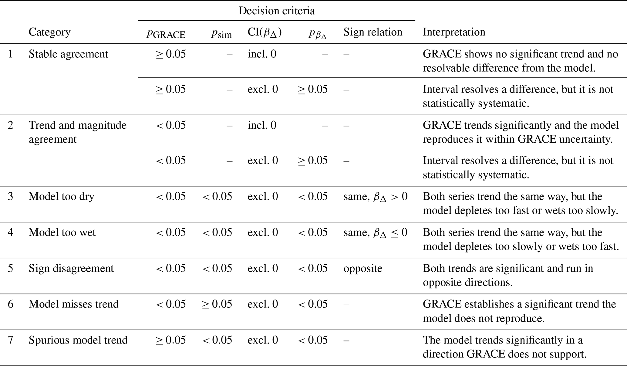
Therefore, to determine whether GLOBGM TWSA is significantly different from GRACE/GRACE-FO, we look at the difference time series (${\mathrm{\Delta }}_{\mathrm{TWSA}}={\mathrm{TWSA}}_{\mathrm{GRACE}}-{\mathrm{TWSA}}_{\mathrm{GLOBGM}}$) and calculate the trend using the Theil-Sen estimate (β_Δ) and significance ($p_{{\mathit{\beta }}_{\mathrm{\Delta }}}$) using the modified Mann-Kendall test (Hamed and Ramachandra Rao, 1998). The influence of GRACE/GRACE-FO uncertainty on β_Δ is incorporated through Monte Carlo sampling from which we calculate the 95 % confidence interval (CI(β_Δ)). In addition, we determine the significance of the GRACE/GRACE-FO TWSA Theil-Sen slope (p_GRACE). These statistics are then used to differentiate between regions which are stable and in agreement, trends and magnitudes agree, model too dry, model too wet, and sign disagreement (Table 4).

Table 4 Classification of grid-scale agreement between GRACE/GRACE-FO and GLOBGM terrestrial water storage trends. p_GRACE: significance of GRACE/GRACE-FO TWSA Theil-Sen slope. p_sim: significance of GLOBGM TWSA Theil-Sen slope. CI(β_Δ): 95 % confidence interval of the difference time-series Theil-Sen slope. $p_{{\mathit{\beta }}_{\mathrm{\Delta }}}$: significance of the difference time-series Theil-Sen slope.

2.4.3 Machine Learning Bias Correction

To correct for systematic bias in simulated water table depths, a machine learning-based bias (ML bias) correction approach was implemented. A Light Gradient-Boosting Machine model (Ke et al., 2017) was trained to predict mean annual bias (Eq. 12) in observed groundwater heads from historical reference simulations (see Sect. 2.3). Observations were obtained from IGRAC's Global Groundwater Monitoring Network (IGRAC, 2024) and included all available annual observation wells (96 799) that overlapped with the simulation period; if multiple wells were located within a single grid cell, the one with the most data was retained. As features, a select number of GLOBGM input parameters (steady-state water table depth, drain conductance, elevation, slope, model layer, recharge, abstraction) and Google's AlphaEarth Foundations geospatial embeddings (Brown et al., 2025) were used. In addition, absolute latitude was added as a proxy for aridity. Observations were split into training (80 %), validation (10 %), and test (10 %) sets using K-means clustering (n = 300) on normalized geographic coordinates, thereby ensuring spatial independence and preventing spatial autocorrelation from inflating performance metrics. Gain-based feature importance scores were calculated for each stage separately, and the importance scores were normalized to enable comparison between the stages.

$$\begin{array}{}\text{(12)}& {\stackrel{\mathrm{‾}}{\mathrm{Bias}}}_{\mathrm{HDS}}={\displaystyle \frac{\mathrm{1}}{n}}\sum _{i=\mathrm{1}}^n\left({\mathrm{HDS}}_{\mathrm{sim},i}-{\mathrm{HDS}}_{\mathrm{obs},i}\right)\end{array}$$

where HDS_sim is the simulated groundwater head and HDS_obs is the observed groundwater head.

We implemented a two-stage ensemble: (1) a binary classifier to predict whether bias is positive ($p_{\mathrm{sign}}=P({\stackrel{\mathrm{‾}}{\mathrm{Bias}}}_{\mathrm{HDS}}>\mathrm{0})$), and (2) a magnitude regressor to predict absolute bias magnitude. For the binary classifier, the bias target was converted into a binary classification target using the indicator function $y_{\mathrm{sign}}=\mathbb{I}({\stackrel{\mathrm{‾}}{\mathrm{Bias}}}_{\mathrm{HDS}}>\mathrm{0})$, and was trained using a binary log-loss metric. Although trained on the log-loss metric, performance is also reported in terms of the proportion of observations where the sign was correctly predicted. For the magnitude model, the target is the log-transformed absolute bias ($y_{\mathrm{mag}}=\log (\mathrm{1}+|{\stackrel{\mathrm{‾}}{\mathrm{Bias}}}_{\mathrm{HDS}}\left|\right)$) and is evaluated using RMSE. For the final bias prediction, the predictions of sign probability and magnitude were combined (Eq. 13). When the sign classifier is uncertain (p_sign(x)≈0.5), the coefficient s(x) approaches zero and the predicted bias is attenuated toward zero, so no full correction is applied where the direction of the bias is ambiguous.

$$\begin{array}{}\text{(13)}& \begin{array}{rl}\widehat{b}& =s\left(\mathit{x}\right)\cdot \widehat{m}\left(\mathit{x}\right)\\ & =\left[\mathrm{2}{p}_{\mathrm{sign}}\right(\mathit{x})-\mathrm{1}]\cdot \widehat{m}\left(\mathit{x}\right)\end{array}\end{array}$$

where s(x) is the prediction from the sign classifier (stage 1) and $\widehat{m}\left(\mathit{x}\right)$ is the prediction from the magnitude regressor.

The trained two-stage model was then used to predict the bias for all grid cells in the model domain, which was then applied to bias-correct GLOBGM v1.1 groundwater heads and water table depths described in Sect. 2.3. To prevent overcorrections and preserve original model physics, an asymmetric ramp-factor correction scheme is implemented (Eq. 14). This approach applies a damping ramp exclusively when the predicted correction would raise the simulated head toward the land surface. In cases where the correction lowers the simulated head, no physical land-surface boundary is at risk of being breached, and thus the full correction is applied without restriction. Finally, the correction was applied to the simulated heads and water table depths (Eqs. 15 & 16).

$$\begin{array}{}\text{(14)}& \begin{array}{rl}& \mathit{\omega }=\left\{\begin{array}{ll}\mathrm{0},& \text{if }min\left({\mathrm{WTD}}_{\mathrm{sim}}\right)\le d_{\mathrm{protect}},\\ \frac{min\left({\mathrm{WTD}}_{\mathrm{sim}}\right)-d_{\mathrm{protect}}}{w_{\mathrm{ramp}}},& \text{if }{d}_{\mathrm{protect}}<min\left({\mathrm{WTD}}_{\mathrm{sim}}\right)<w_{\mathrm{ramp}},\\ \mathrm{0.9},& \text{if }min\left({\mathrm{WTD}}_{\mathrm{sim}}\right)\ge w_{\mathrm{ramp}},\end{array}\right.\\ & \mathrm{\Delta }{d}_{\mathrm{correction}}=\left\{\begin{array}{ll}\widehat{b}\mathit{\omega },& \text{if }\widehat{b}<\mathrm{0},\\ \widehat{b},& \text{if }\widehat{b}\ge \mathrm{0}.\end{array}\right.\end{array}\end{array}$$

where d_protect is a protection depth below which no correction is applied (0.1 m) and w_ramp is the ramp width over which the correction scales from 0 to 0.9 (2 m).

$$\begin{array}{}\text{(15)}& {\displaystyle }{\mathrm{HDS}}_{\mathrm{corrected}}\left(t\right)={\mathrm{HDS}}_{\mathrm{sim}}\left(t\right)-\mathrm{\Delta }{d}_{\mathrm{correction}}\text{(16)}& {\displaystyle }{\mathrm{WTD}}_{\mathrm{corrected}}\left(t\right)={\mathrm{WTD}}_{\mathrm{sim}}\left(t\right)+\mathrm{\Delta }{d}_{\mathrm{correction}}\end{array}$$

2.5 GLOBGM v1.1 in comparison to previous modeling efforts

To assess model performance in relation to previous global modeling efforts, we benchmarked GLOBGM against existing global groundwater models. This allows us to assess the model skill relative to the current state-of-the-art and identify where improvements have been achieved. We compared the steady state GLOBGM v1.1 results with those of Fan et al. (2017), de Graaf et al. (2017), Reinecke et al. (2019) and Verkaik et al. (2024). For the transient simulation, GLOBGM v1.1 was compared to Verkaik et al. (2024) and de Graaf et al. (2017).

To compare inter-model performance for steady state estimates, we calculated the absolute bias between observations and simulated water table depth. However, for the transient simulations we used the KGE-NP_skill with reference to the mean flow benchmark. Given that the models used for comparison are at the 5 arcmin (de Graaf et al., 2017; Reinecke et al., 2019) and 30 arcsec resolution (Fan et al., 2017; Verkaik et al., 2024), to compare the models in a pragmatic manner, we calculated the validation metrics on the observations described in Sect. 2.4.2, which are geared towards the validation of a 30 arcsec grid. For these comparisons, GLOBGM v1.1 is represented by its raw uncorrected outputs and for transparency, we also report the optional ML-corrected product (ML-GLOBGM v1.1).

2.6 Analysis

To provide insights into the spatial distribution of groundwater at the 30 arcsec resolution and highlight the benefit of increased resolution the long-term average annual groundwater table depth was calculated at the global scale (Eq. 17). For visualization purposes, a “from ground level downwards” view of groundwater table depths is provided; for locations where a confining layer exists, only the top model layer is visualized.

$$\begin{array}{}\text{(17)}& {\stackrel{\mathrm{‾}}{\mathrm{WTD}}}_{i,j}={\displaystyle \frac{\mathrm{1}}{\mathrm{12}N}}\sum _{k=\mathrm{1}}^N\sum _{m=\mathrm{1}}^{\mathrm{12}}{\mathrm{WTD}}_{i,j,k,m}\end{array}$$

where ${\stackrel{\mathrm{‾}}{\mathrm{WTD}}}_{i,j}$ is the average WTD at grid point (i,j), N is the total number of years, m is the month index, and ${\mathrm{WTD}}_{i,j,k,m}$ is the WTD at grid point (i,j) in month m of year k.

To analyze how groundwater resources have changed in the past and may change in the future, we estimated trends in water table depth using the Theil-Sen estimator (Sen, 1968; Theil, 1950) so that the slope for each cell was calculated along the time dimension as the median of all pairwise slopes between distinct time points (Eq. 18). We tested the slopes for each grid cell using the Mann-Kendall test (Kendall, 1975). When presented as a raster, slopes less than 0.001 m yr⁻¹, not statistically significant at the 95 % confidence level, or both were masked. For visualization purposes, only the bottom layer of the model is presented, which represents fully unconfined aquifers or confined aquifers.

$$\begin{array}{}\text{(18)}& m_{i,j}=\mathrm{median}\left\{\left.{\displaystyle \frac{\mathrm{HDS}(t_l,i,j)-\mathrm{HDS}(t_k,i,j)}{t_l-t_k}}\right|\forall k<l\right\}\end{array}$$

where m_i,j is the median slope at grid point (i,j), $\mathrm{HDS}(t_k,i,j)$ is the value of HDS at time t_k and grid point (i,j). The median is taken over all pairs of time indices k<l.

In addition, we present the slopes of mean water table depth aggregated by spatial units. The spatial units are combined water provinces (Straatsma et al., 2020) and WHYMAP aquifer dataset (Chen et al., 2017). We first computed, for each spatial unit and each year, the area-weighted mean water table depth over all cells within that unit, and then applied Eq. (18) and the Mann-Kendall test to aggregated time series. For the spatially aggregated representation, slopes less than 0.001 m yr⁻¹, not statistically significant at the 95 % confidence level, or both were masked. To complement the trends, we calculated area-weighted mean water table depth anomalies, relative to 1965, over the simulation period aggregated by continent.

3 Results

3.1 Calibration, Spin-up and Initial Conditions

3.1.1 Calibration

GLOBGM proved sensitive to adjustments in hydraulic conductivity, anisotropy, and entrance resistance (Table 5 & Fig. 2e). Among the top ten calibration combinations, candidate 1 achieved the lowest mean absolute bias overall, for the 0–5 m and 10–20 m categories, and the second lowest in the 5–10 m category (Table 5). Consequently, a prefactor of 0.1 for all parameters was chosen as the best set. The selection of these prefactors correspond to the minimum values tested, which suggests that smaller prefactors may have provided better performance. However, the range of calibration factors was intentionally constrained within two orders of magnitude to avoid significant deviations from the original parameterization and prevent overfitting.

Table 5 Comparison of the top 3 calibration candidates (ordered by mean absolute depth-weighted bias) against the reference GLOBGM v1.0 benchmark. Parameter settings are dimensionless multipliers applied to the default values. Values in bold indicate the chosen calibration settings.

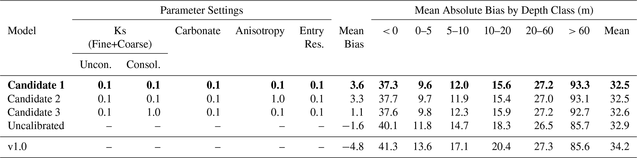
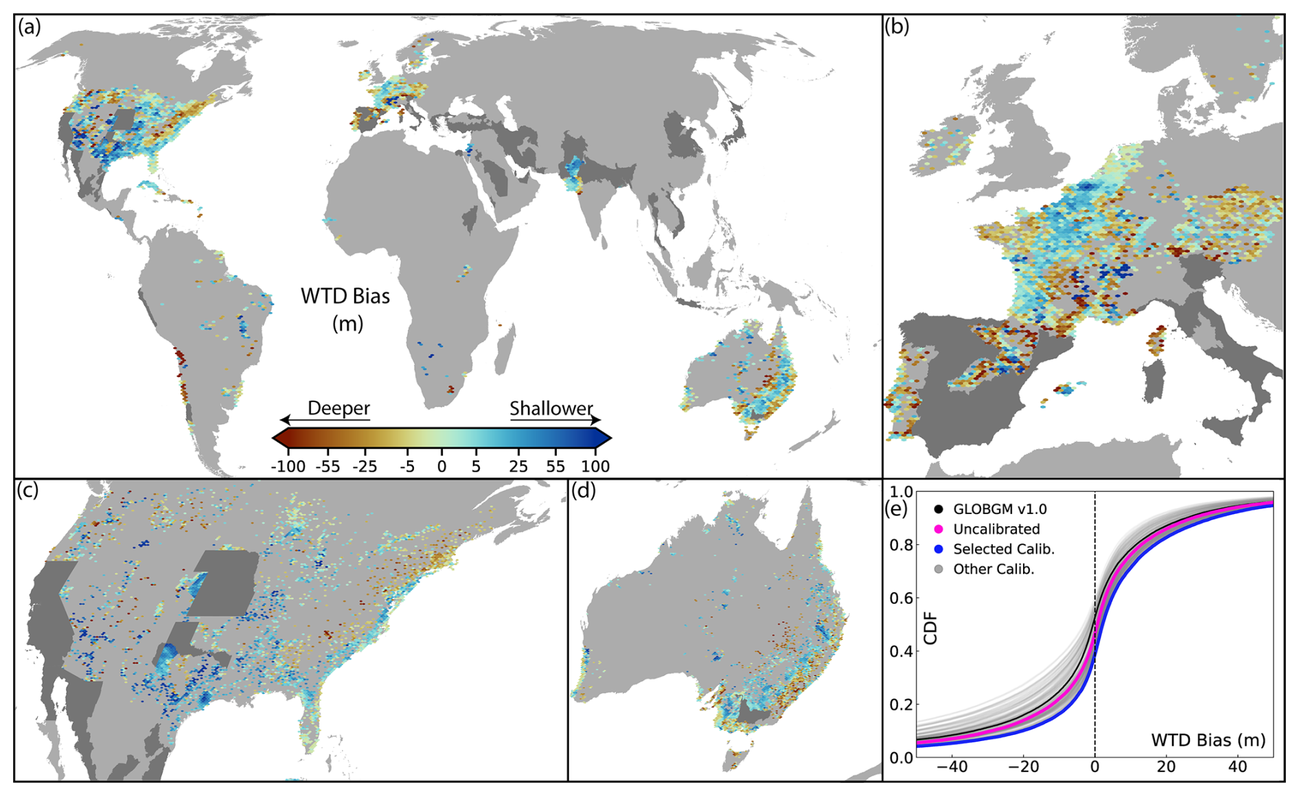
Figure 2 (a) Geographical variation of water table depth bias, for the chosen calibration setting, from 34 800 observation wells that were used to assess different calibration settings. Dark grey polygons indicate regions of known anthropogenic influence on the water system and were excluded from the calibration. With zoomed insets of (b) western Europe, (c) United States, (d) Australia. (e) Cumulative distribution function of the water table depth bias of the 162 calibration permutations.

Greater variance among permutations was observed for locations where simulated water table depths are deeper than observed. This suggests that calibration influenced over-estimated depths more significantly than under-estimated ones (Fig. 2e). Varying calibration prefactors tended to shift entire distributions rather than simultaneously correcting outliers at both ends (Fig. 2e). As a result, the chosen prefactor set improved the accuracy of over-estimated depths but increased the error for under-estimated depths. However, this set maintained the best overall bias, as gains at the negative end of the distribution were offset by penalties at the positive end (Table 5 & Fig. 2e). Compared to the previous uncalibrated GLOBGM v1.0 (Verkaik et al., 2024), the chosen calibration settings display marked reductions in overall depth weighted bias (Table 5). This is especially prevalent for shallower water table depths (< 20 m; Table 5). For wells between 20 and 60 m calibration has little effect, whereas for wells deeper than 60 m calibration increased bias (Table 5). In comparison to GLOBGM v1.0, unweighted bias shifts from a tendency to overestimate water table depths (−4.8 m) to underestimation when calibrated (3.6 m) (Table 5 & Fig. 2e). Comparing the uncalibrated GLOBGM v1.1 with v1.0 reveals how the dynamic elevation routine and groundwater recharge downscaling affect the model's accuracy. Compared to GLOBGM v1.0, the uncalibrated v1.1 predictions were closer to the ideal bias score of zero, by a magnitude of 1.6 m, again centered around improvements in simulations that were deeper than observed (Table 5 & Fig. 2e).

3.1.2 Spin-up and Initial Conditions

The objective of the first transient spin-up step was to achieve dynamic equilibrium for the year 1960, whereas the second step incorporated abstraction to reproduce expected water table depths. The key assumption is that initiating the simulation from a naturalized steady state solution and simulating 1960 iteratively, without abstraction, would yield water table depths which are shallower than observed; therefore, by activating abstraction in the second step, water table depths would approach observed values. During the first step, the change in average groundwater heads between successive iterations decreased – suggesting the model approached dynamic equilibrium. The correlation-based analysis aimed at detecting regions where the model was not properly spun up reveals that the majority of grid cells were correctly initiated at the start of the simulation. Regions that were incorrectly initiated were sparse and geographically confined. Most regions reached adequate spin-up within the first 5 years, with 99.7 % of the domain deemed valid after the first year, 99.8 % after the second year, 99.9 % thereafter, and 99.99 % by 1965 (Fig. 3b).

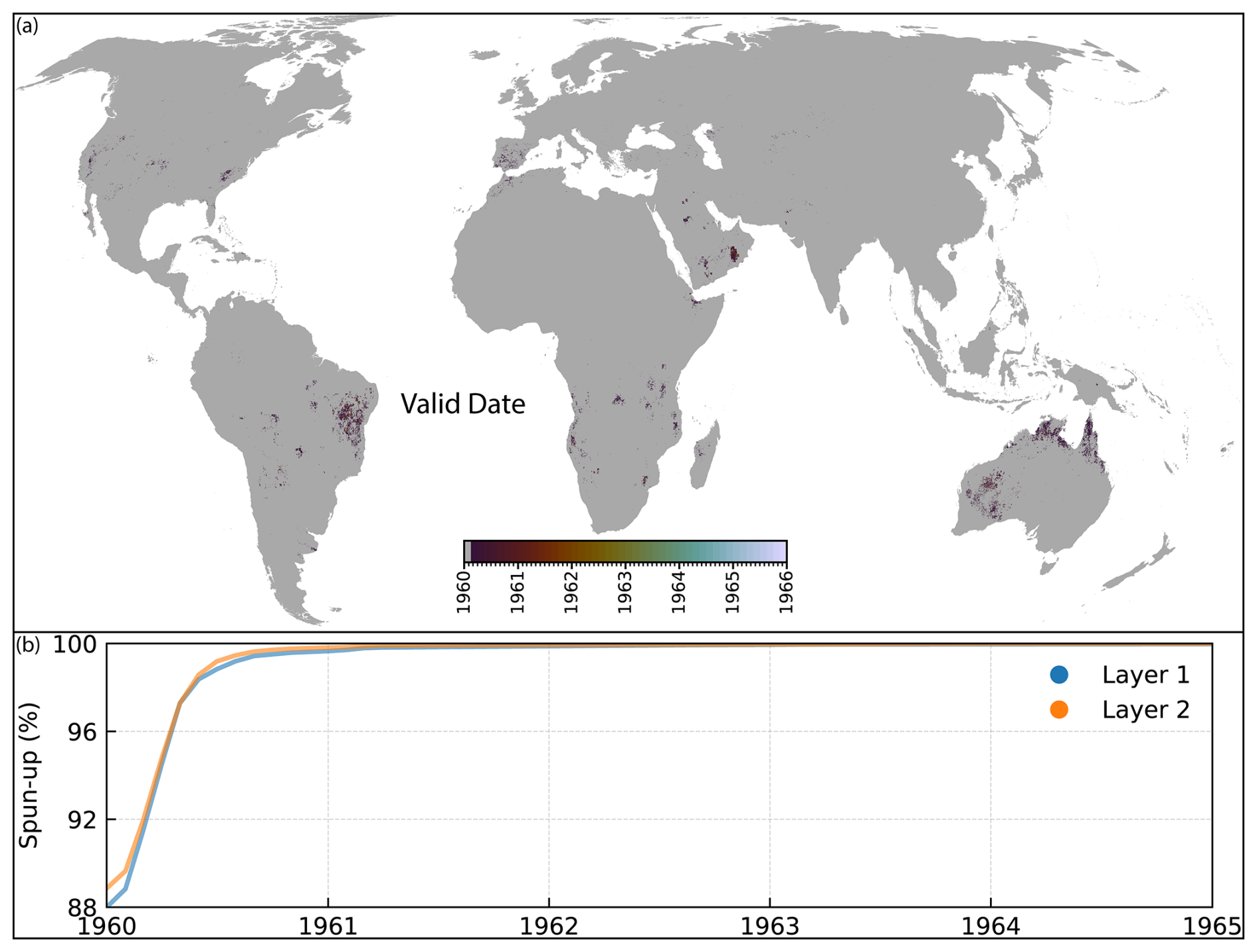
Figure 3 (a) Map showing the first year of valid simulation data per grid cell. (b) Percentage of grid cells in Layer 1 and Layer 2 that are free of spin-up artifacts between 1960 and 1965.

3.2 Quality Assurance, Validation and Bias Correction

3.2.1 Quality Assurance

Previous evaluations of the 5 arcmin predecessor of GLOBGM v1.1 have revealed that performance degrades in regions where geology is dominated by karst aquifers, permafrost, or mountainous terrain (Fig. 4) due to incomplete process representation. GLOBGM performs better in sedimentary than in karst basins, presumably because the Darcian flow assumption is questionable in karst settings (de Graaf et al., 2017; Verkaik et al., 2024). In mountainous regions, GLOBGM models groundwater heads within mountain blocks but does not parametrize water bodies in hillslopes and smaller alluvial mountain valleys, since the hydrogeological schematization is too coarse. Moreover, it is assumed that the secondary permeability of fractured hard rock in mountainous regions can also be represented by the principles of Darcian groundwater flow (Verkaik et al., 2024). Research into the applicability of PCR-GLOBWB2 to simulate the hydrology of permafrost regions shows that it does not capture the dynamics of permafrost with high fidelity due to its simplified representation of ice melt (i.e., degree-day-factor) and lack of dynamic permafrost schemes, which leads to underestimated discharge and, consequently, groundwater recharge (Gädeke et al., 2020). Moreover, it is challenging to define groundwater resources in areas where soil is frozen up to many tens of meters deep (Diak et al., 2023; Cochand et al., 2019). These masks are provided, together with the simulations, to inform users of regions where GLOBGM v1.1 predictions are likely less reliable.

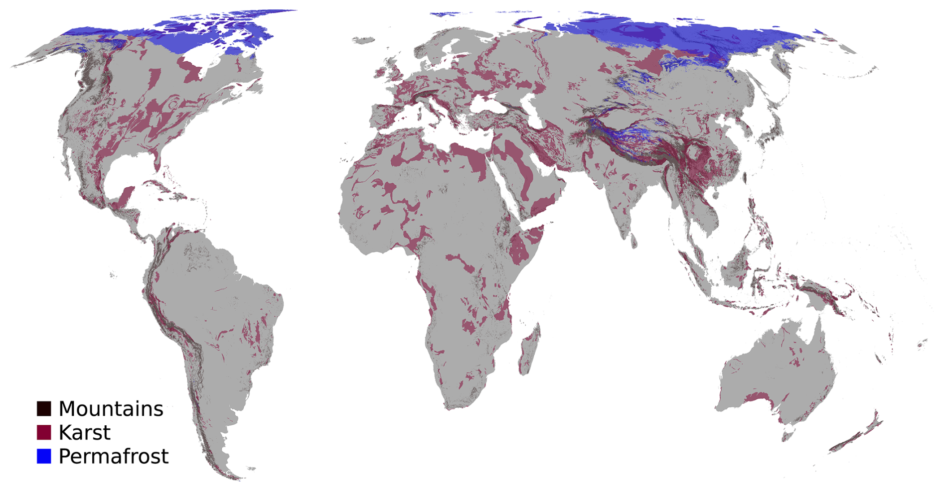
Figure 4 Regions where GLOBGM has process representation limitations due to practical and theoretical limitations; namely, karst aquifers, permafrost and mountainous regions.

3.2.2 Validation

When validating on the uncorrected simulations, monthly scores (74.7 % KGE-NP_skill>0) are generally higher than annual (67.0 % KGE-NP_skill>0) scores (Fig. 5a, e). This trend is also evident in the constituent components of KGE-NP, where correlations are generally higher when validated at monthly scales (Fig. 5c, g). Variability and bias show no difference between monthly and annual resolutions (Fig. 5d, e, h, i). The ability of GLOBGM to simulate groundwater heads varies predictably with water table depth. KGE-NP_skill scores grouped according to depth categories reveal that the deeper simulations (> 60 & 20–60 m) are the worst performing, with approximately 56 %–70 % displaying skillful predictions that improve upon the mean flow benchmark (Fig. 5b, f). Shallower observations (0–20 m) are better reproduced, with 68 %–80 % of locations showing skillful predictions (Fig. 5b, f). This depth-dependent pattern is also evident in correlation reproduction, where shallower values are more accurately predicted than deeper values (Fig. 5c, g). Groundwater heads tend to be underestimated for observations between 0–5 m (Fig. 5e, i). In contrast, groundwater heads are over-estimated for deeper water table depths (Fig. 5e, i). In contrast, the ability to reproduce variability shows no clear correlation with water table depth (Fig. 5d, h).

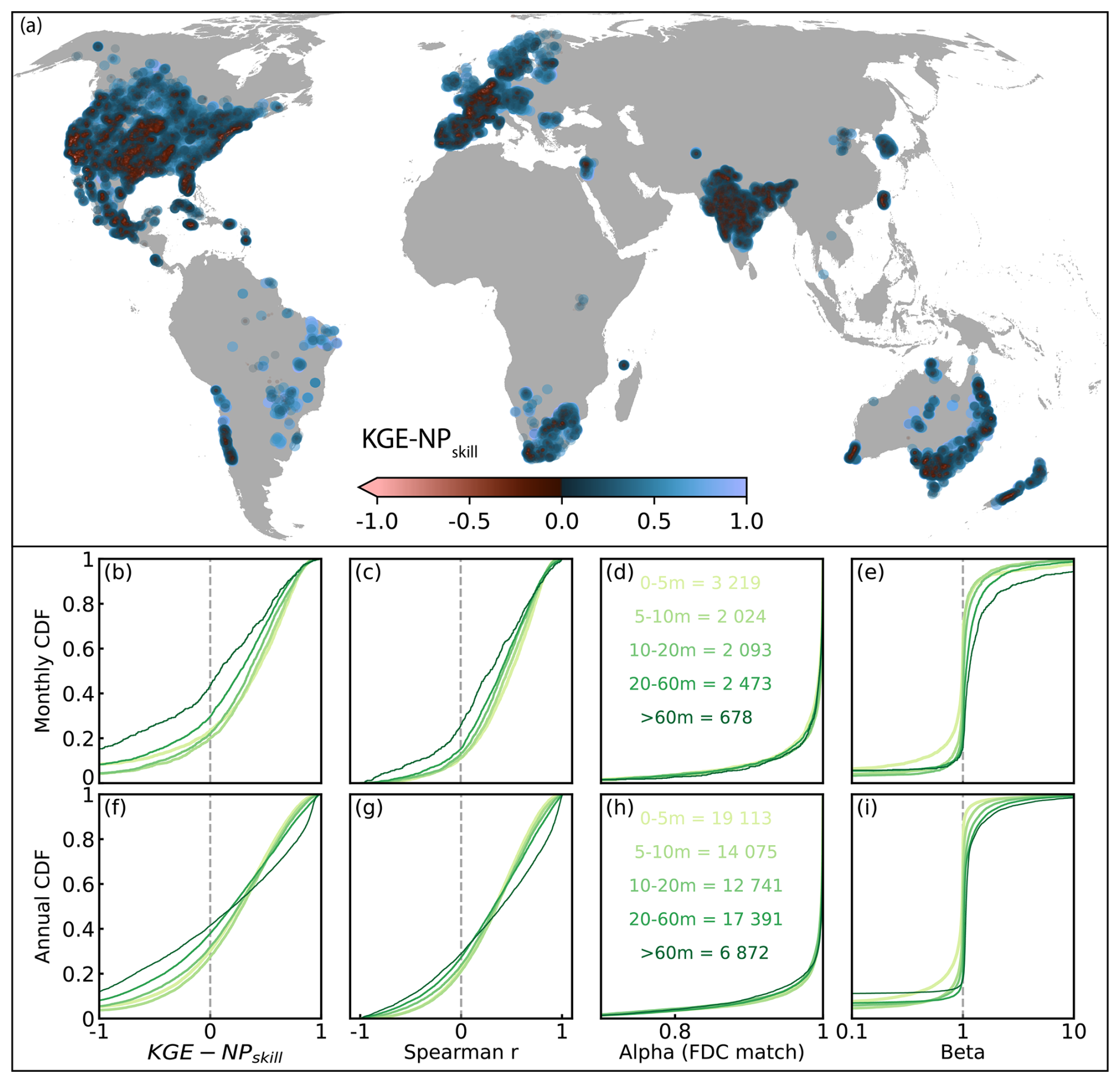
Figure 5 KGE-NP_skill spatial distribution (a) and CDF (b, f). Constituent components (c, g) correlation, (d, h) alpha, and (e, i) beta of KGE-NP for monthly and annual groundwater heads simulated by GLOBGM from 1965–2019, grouped by water table depth. Gray lines in panels (b) and (f) symbolize a KGE-NP_skill of 0 which is the threshold at which greater values indicate predictions that improve upon the mean flow benchmark. Gray lines in panels (c) and (g) indicate the point at which correlations are positive to the right and negative to the left. Gray lines in panels (e) and (i) separate over-estimation to the right and under-estimation to the left.

To determine whether low performance scores at specific locations reflect genuine physical discrepancies or arise from evaluation metrics artifacts and whether performance varies between stable or trending observed time series, we conducted a post-hoc analysis. Where trends are present (|Theil-Sen slope| > 0.01 m yr⁻¹) in the observed time series, 83 % (monthly) and 73 % (annual) of the locations are skillful, compared to 78 % (monthly) and 70 % (annual) where observed time series is considered stable (|Theil-Sen slope| ≤ 0.01 m yr⁻¹; Fig. D1). The overall KGE-NP_skill score is mainly impacted by small values in the denominator of the bias ratio (β), which is caused by small groundwater heads. Removing these cases (μHDS_obs<1.0 m) means 80 % of the monthly and 71 % of the annual scores are skillful, an improvement of 5 and 4 percentage points in the monthly and annual validations, respectively (Fig. D2).

The spatial variation in KGE-NP_skill score corroborates some of the conclusions derived from the cumulative distribution functions (Fig. 5a). For instance, lower scores are evident along regions where water table depths are expected to be deeper, such as arid regions and mountainous terrain (Fig. 5a). Furthermore, depth-dependency becomes evident when comparing relatively lower scores in the higher elevations of the Appalachian, Pyrenees, and Great Divide mountains to higher scores in the adjacent low lying regions (Fig. 5a). Similarly, the higher regions of the Indo-Gangetic Plain display lower KGE-NP_skill scores when compared to coastal regions (Fig. 5a). Figure 5a and the analyses shown in Fig. D3 show that the regions of poor performance do not line up well with the regions in Fig. 4 where GLOBGM is expected to provide less accurate results due to limitations in process representation. In addition, there are no significant differences in performance between locations outside or inside major abstraction areas (Fig. D3).

The spatial distribution of TWSA trends shows broad-scale agreement between GLOBGM and GRACE/GRACE-FO (Fig. E1a). GLOBGM matches GRACE/GRACE-FO in both trend direction and magnitude for 45.7 % of the world (Fig. E1a). The two agree in direction but disagree in magnitude over 16.6 %; GLOBGM is too wet over 9.8 % and too dry over 6.8 % (Fig. E1a). GRACE/GRACE-FO disagree in direction for only 7.1 % (Fig. E1a). Over 17.8 % GRACE/GRACE-FO indicates a significant trend where GLOBGM simulates no trend. Conversely, GLOBGM simulates a trend when GRACE/GRACE-FO indicates no trend over 12.8 % of the world. GLOBGM simulates the direction of TWSA trend in known regions of water storage decline, such as the south-western United States, northern India, and Pakistan, and the Middle East (Fig. E1). Lack of agreement aligns with karst, permafrost, and mountainous regions (Fig. E1); GLOBGM is expected to show reduced accuracy in these regions (Sect. 3.2.1). Notable examples include the Arctic, sub-Arctic regions North America and eastern Russia, where permafrost is present. Furthermore, disagreement is evident across prominent mountain ranges like the Andes and the Himalayas are evident (Fig. E1). Model disagreement is also evident in major karst landscapes. This is particularly evident across Mexico, Northern Africa, the Gulf of Guinea, and the Tibetan Plateau (Fig. E1). In addition, disagreement is prevalent in islands and around the world's major water bodies, such as the Great Lakes, Rift Valley Lakes, and Caspian Sea (Fig. E1).

3.2.3 Machine Learning Bias Correction

The machine learning based bias correction demonstrated adequate performance on the holdout set. The binary sign classifier was capable of correctly predicting bias direction in 80 % of the cases, which was comparable to the validation (80 %) and train (90 %; Table F1) sets. Similarly, the magnitude regressor achieved an RMSE of 37.4 in the train set, which was comparable to the validation (25.3) and test (36.7; Table F1) sets. The steady-state depth of the water table emerges as the most important feature (Fig. F1a, b). The ML-corrected GLOBGM estimates show a predominantly negative bias for central North America and Europe (Fig. 6a); whereas, the Indian subcontinent and semi-arid regions of southern Africa display a positive bias (Fig. 6a).

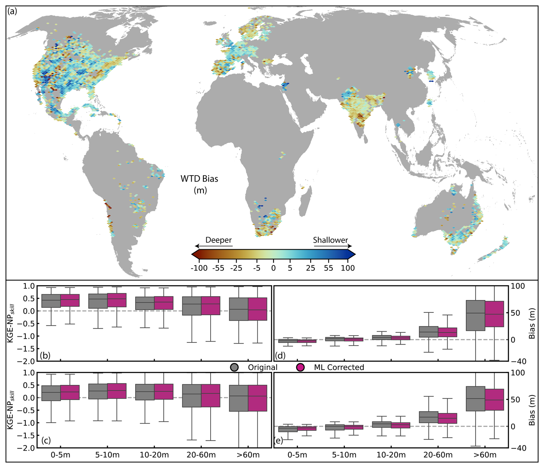
Figure 6 (a) Spatial distribution of ML-corrected mean water table depth bias (m). Original and ML-corrected (b) monthly and (c) annual KGE-NP_skill scores, calculated from heads, grouped by water table depth classes. Original and ML-corrected (d) monthly and (e) annual mean water table depth bias (m) across the same water table depth classes.

When grouped by depth classes, the original model showed a consistent pattern of over-estimation for shallower wells (0–10 m) and under-estimation for deeper wells (> 20 m; Fig. 6d, e). The ML correction reduced the median bias across all depth classes and improved the bias for the majority of the locations (Figs. 6d, e & F1c, d). After ML correction, the median bias shifted closer to zero in all categories and the interquartile range contracted (Fig. 6d, e). This reduction was particularly notable for the class > 60 m, where the original model showed the largest biases (Fig. 6d, e). The bias correction was more effective on the annual time scale compared to the monthly time scale, with a more pronounced reduction in bias (Fig. 6d, e). Post correction bias reductions translated into improved KGE-NP scores. For both the annual and monthly time scales, the ML-corrected simulations displayed higher median KGE-NP scores and reduced interquartile ranges across all depth classes (Fig. 6 b, c). These improvements led to a ∼ 0.3 %–1.7 % increase in the proportion of observations with skillful predictions (KGE-NP_skill>0; Fig. F1e).

3.3 GLOBGM v1.1 in comparison to previous modeling efforts

The raw steady-state GLOBGM v1.1 estimates are comparable to previous global 30 arcsec resolution efforts (GLOBGM v1.0 & Fan et al., 2017; Fig. 7a, b). Although Fan et al. (2017) achieves the lowest mean absolute bias overall (18.11 m), the CDFs intersect at approximately 20 m, indicating a lack of overall dominance. GLOBGM v1.0 and GLOBGM v1.1 exhibit a higher proportion of sites with absolute bias below 20 m, yet above this threshold Fan et al. (2017) provide more accurate estimations. This crossover suggests that Fan et al. (2017) achieves its lower mean absolute bias primarily through superior performance at locations with moderate-to-large errors, while GLOBGM v1.1 more effectively captures water table depth at the majority of locations (approximately 75 %) but at the cost of a heavier error tail (Fig. 7a, b). Applying the optional machine-learning bias correction (ML-GLOBGM v1.1) reduces the absolute bias further relative to observations (Fig. 7a, b).

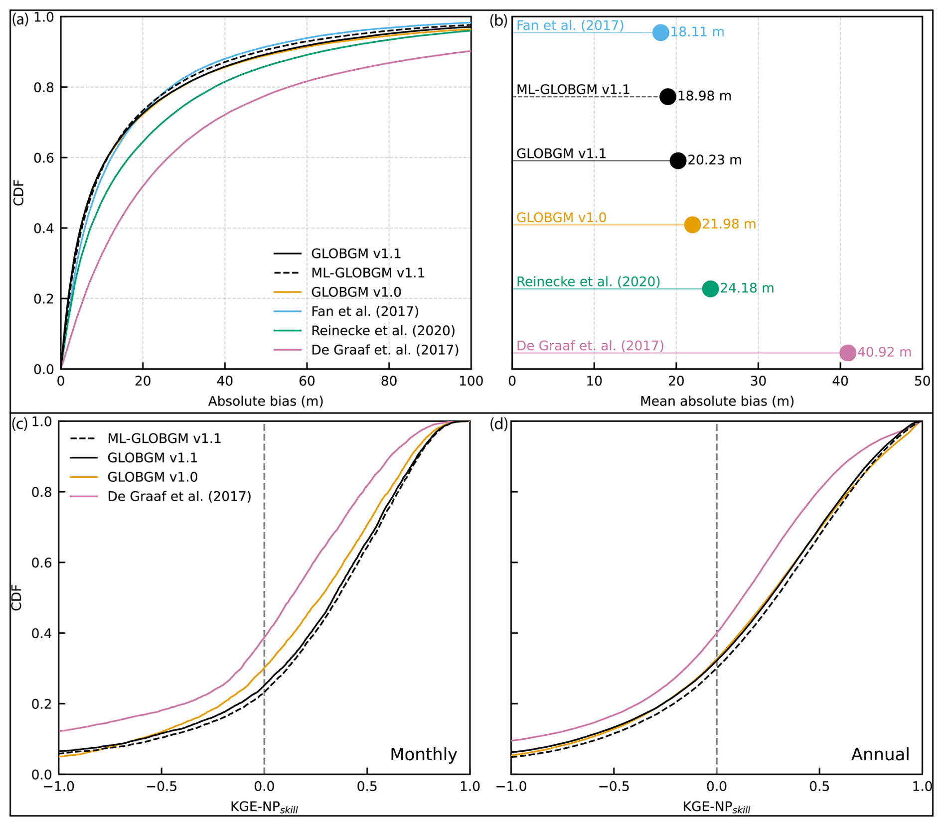
Figure 7 (a) CDF and (b) mean absolute bias in simulated steady-state water table depth validated against observations. (c) Monthly and (d) annual KGE-NP_skill scores for transient simulated hydraulic heads validated against observations.

Compared to the 5 arcmin counterparts (de Graaf et al., 2017) the 30 arcsec simulations show marked improvements (Fig. 7c, d). Collectively, different versions of GLOBGM display an approximately 19 and 15 percentage points increase in the number of locations that improve upon the mean benchmark (KGE-NP_skill>0), at the monthly and annual resolution respectively (Fig. 7c, d). The raw uncorrected GLOBGM v1.1 simulation represents an improvement over v1.0, particularly at the monthly resolution, 8 and 1 percentage points increase at the monthly and annual resolution, respectively (Fig. 7c, d). The ML-correction provides further improvement (Fig. 7c, d).

3.4 Historical Reference Simulation

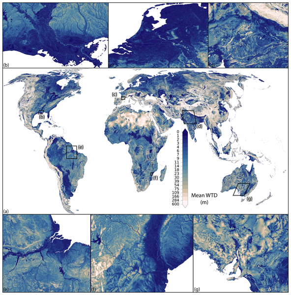
The hyper-resolution groundwater model reveals the added spatial detail in mean annual water table depth (Fig. 8a). Finer scale interactions between river systems and groundwater are evident at this hyper-resolution. For example, the shallow reaches of the Amazon and Mississippi rivers, with their respective deltas, are visible through shallow water tables (Fig. 8e, b). Other major deltas, like the Indus and Ganges-Brahmaputra (Fig. 8d), are also well resolved at this resolution and shallower water table depths along the coast compared to more interior regions are present (Fig. 8b–g). Average water table depths largely resemble our current broad understanding of groundwater dynamics and reflect the influences of precipitation, topography and geology on driving the distribution of groundwater reserves.

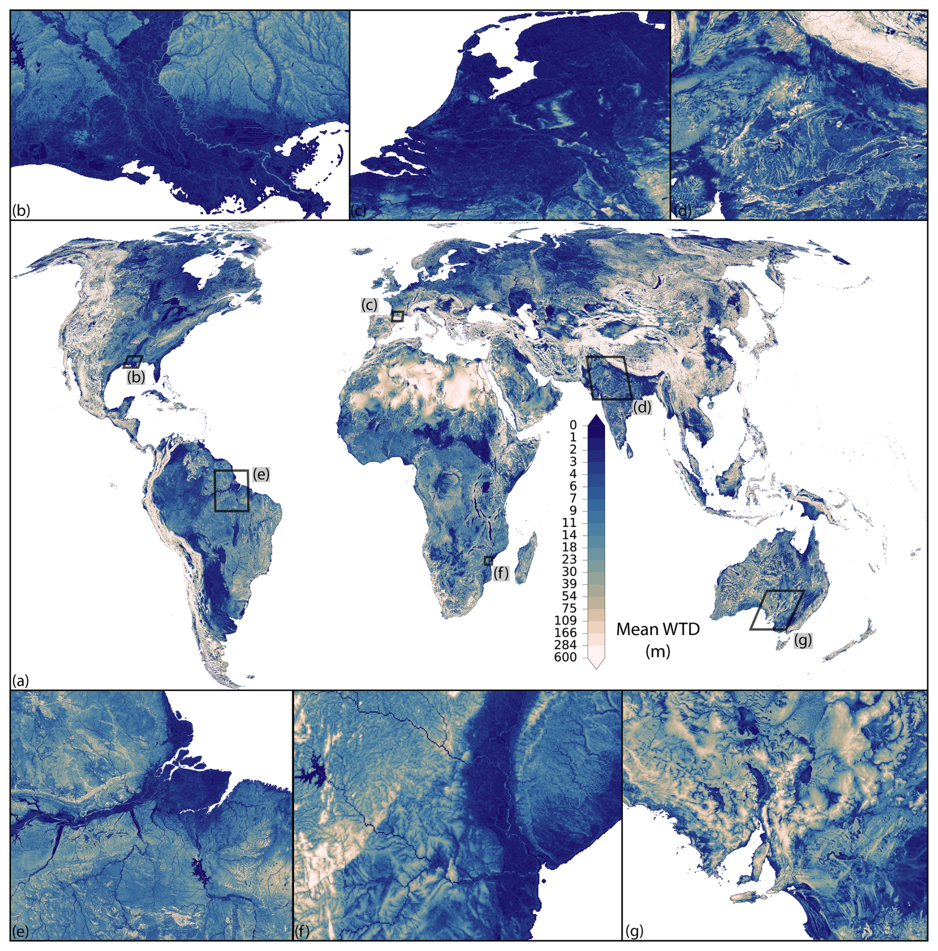
Figure 8 (a) Mean annual water table depth (1965–2019) simulated by GLOBGM. With zoomed insets providing more detail over (b) the Mississippi delta, (c) Netherlands, (d) Indo-Gangetic Plain, and (e) the Amazon basin, (f) Zambezi delta and (g) Southern Australia. In areas where a confining layer is present, only the uppermost model layer is depicted, thus providing a perspective from the ground surface downward.

Water table depths are seen to be deeper in the arid regions and shallower in humid areas, reflecting the difference in groundwater recharge rates which are driven by large-scale precipitation patterns (Reinecke et al., 2024). More mountainous regions exhibit deeper water table depths which is expected given the relatively lower infiltration rates, lower permeability, and tendency for water to move down slope by streams towards lower lying ground under the influence of gravity (Somers and McKenzie, 2020). GLOBGM reproduces deepening water table depths in regions where groundwater depletion is known to occur, such as the southern and central High Plains in the United States (Figs. 9 & G1), Iran (Figs. 9 & G1), Indo-Gangetic Plain (Figs. 9 & G1; Jasechko et al., 2024). Interestingly, GLOBGM identifies a number of regions where water table depths have risen, the majority of which are located in the northern latitudes and Arctic Circle, such as Northern Scandinavia and the Russian Far North. This could conceivably be due to climate change enhancing precipitation and groundwater recharge dynamics; however these trends align with permafrost regions where GLOBGM has been shown to be less reliable (McKenzie et al., 2021). In addition, simulated rising water tables match regions that have been shown to display increases in groundwater reserves such as the Guarani aquifer in South America, the northern Great Plains in North America, and the Karoo Basin in South Africa (Figs. 9 & G1; Jasechko et al., 2024; Taylor et al., 2013).

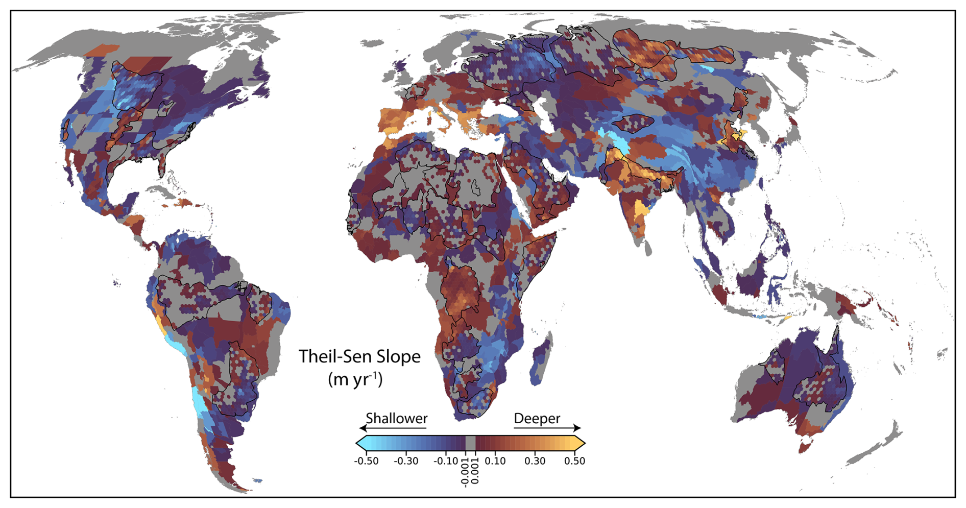
Figure 9 Theil-Sen slope of annual water table depth (1965–2019) simulated by GLOBGM. Gray pixels indicate regions where slopes are either insignificant, less than 0.001 m yr⁻¹, or both. Note that this figure represents the lower model layer which is representative of unconfined and confined aquifers.

3.5 Ensemble-mean Scenario Simulations

The trends in water table depths between 2015 and 2100 show that the different SSP-RCP scenarios do indeed suggest alternative futures for groundwater reserves (Figs. 10 & G2). At the global scale, more regions exhibit rising than declining water table depths (Figs. 10 & G2). The intensity of change and the proportion of areas projected to undergo change differ among the three SSP-RCP scenarios. More specifically, SSP1-RCP2.6 shows the lowest projected rate of change in water table depths, followed by SSP3-RCP7.0, whilst SSP5-RCP8.5 displays the largest projected rate of change (Figs. 10 & G2).

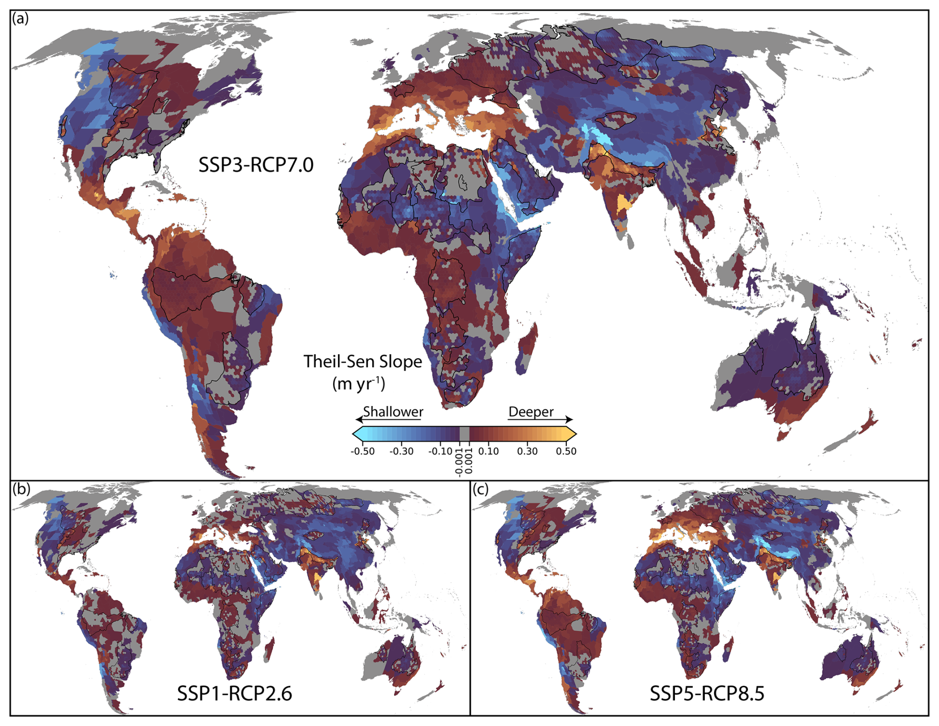
Figure 10 Theil-Sen slope of annual water table depth (2015–2100) simulated by GLOBGM under three SSP-RCP scenarios. Gray pixels indicate regions where slopes are either insignificant, less than 0.001 m yr⁻¹, or both. Note that this figure represents the lower model layer which is representative of unconfined and confined aquifers.

Many regions show consistent directions of change across all three scenarios; however, some differences are evident. The regions in which water table depths are projected to rise are the Sahel, Horn of Africa, North America's Pacific Coast, Tibetan Plateau, Northern Polar regions and Arabian Peninsula (Figs. 10 & G2). In contrast, water table depths are projected to decline in the Mediterranean, south eastern Australia, and the African and South American tropics (Figs. 10 & G2). The Alps and the Amazon are some of the few regions that show divergence in the direction of change. A declining water table depth is projected for the Amazon under SSP3-RCP7.0 and SSP5-RCP8.5, in contrast to a projected stable water table depth under SSP1-RCP2.6. Water table depth in the Alps is projected to rise under SSP1-RCP2.6 and decline under SSP3-RCP7.0 and SSP5-RCP8.5 scenarios (Figs. 10 & G2). Projected trends indicate that water tables will rise across the majority of continents in the coming century (Fig. 11). This rise is persistent in Africa and North America, accelerating under higher emission scenarios (Fig. 11b, d). In Asia, the water table remains relatively stable until the 2010s before beginning to rise, again intensifying with higher emissions (Fig. 11c). Australasia follows a similar upward trajectory before stabilizing around 2050, with minimal variation between scenarios (Fig. 11g). Conversely, Central and South America exhibit early increases followed by a divergence: SSP1-RCP2.6 leads to stability, while the other scenarios result in deepening water tables (Fig. 11e). Small islands show an initial rise until 2010 followed by a decline, with no discernible difference between the scenarios (Fig. 11f). Europe is the distinct outlier; it is the only region where the water table markedly deepens, particularly under higher emission scenarios, while SSP1-RCP2.6 maintains relative stability (Fig. 11a).

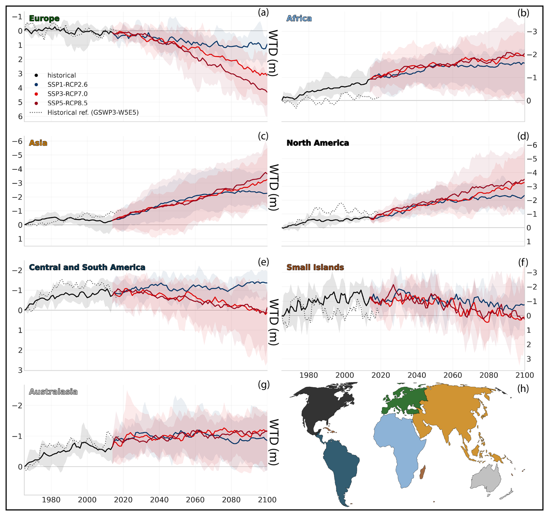
Figure 11 Time series of regional mean WTD (m) anomalies relative to 1965 for the historical-reference, historical and three Shared Socioeconomic Pathways: SSP1-RCP2.6, SSP3-RCP7.0, and SSP5-RCP8.5. Shaded bands depict the spread of the models (min–max). The map in panel (h) defines the aggregation regions.

4 Discussion

4.1 Model Development and Methodological Advances

Compared to its predecessor, GLOBGM v1.1 incorporates four methodological changes: calibration, recharge downscaling, a dynamic elevation routine and an improved spin-up procedure. In addition to the raw model outputs, we also provided a dataset which was bias corrected using a machine learning based method.

The contributions of the dynamic elevation routine and the recharge downscaling routine yielded increased accuracy when compared to the uncalibrated GLOBGM v1.0 and v1.1. Nevertheless, accurate estimation of groundwater recharge remains a challenge in global hydrological modeling, with its estimates varying widely across models due to limited observational data and high spatial heterogeneity of recharge processes (Reinecke et al., 2024; Berghuijs et al., 2024). Working within these limitations, we demonstrate that introducing a relatively simple statistical estimate of recharge at the hyper-resolution yields improved groundwater head estimates. In agreement, recent work has demonstrated that machine learning approaches are capable of predicting recharge fields at the global scale (Jung et al., 2024).

GLOBGM v1.1, calibrated through lithology-specific parameter adjustments, produces simulations with reduced bias and improved spatial agreement with observed water table depths, consistent with findings from regional and global studies reporting performance gains from calibrations (Fan et al., 2013; Zell and Sanford, 2020). However, applying prefactors at the global-scale, or even based on lithological class as done here, shifts the entire distribution. Ideally, calibration would cause the upper and lower tails of the bias distribution to converge toward zero. Using global objective functions and calibration factors that influence large regions with very different hydrological characteristics inherently prevents incorporation of needed regional sensitivity; this is compounded by uncertainties in the datasets used to define lithological groupings and the uneven distribution of observations. Efforts focused on the collection and dissemination of observed groundwater data to broaden the scope and coverage of the current geographically constrained (Fig. C1) large sample datasets are central to achieving realistic parameter estimates through calibration (Jasechko and Perrone, 2021; Bäthge et al., 2026). Future studies should investigate whether alternative calibration techniques such as sequential calibration (Béraud et al., 2024) or data assimilation approaches that incorporate observed data (Béraud et al., 2024; White, 2018) may aid in realizing locally specific calibration sensitivities. Similarly, regionalization and regularization methods have been shown to improve calibration of global hydrological models (Kupzig et al., 2024; Doherty, 2003).

The approach used to estimate initial groundwater heads resulted in a more accurate estimation of initial states than what would have been accomplished had the traditional approach been used (i.e., steady state simulation followed by transient sub-model without abstraction for 20 iterations). Nonetheless, results also suggest room for improvement. Ideally, the model would display strict dynamic equilibrium for all locations; however, this would require a disproportionate amount of computational power to achieve relatively small changes in initial groundwater head estimates. The estimation of accurate and representative initial states is an often cited problem for global groundwater models (Reinecke et al., 2024; de Graaf et al., 2017) and Earth system models in general (Werndl, 2019). Opportunities exist to improve this by using advances in initial condition estimation algorithms, such as those based on sequence acceleration (Khatiwala, 2024) or by making use of artificial intelligence surrogate models where repetitive iterations can be simulated at a faster rate (Asher et al., 2015; Bennett et al., 2024; Pawusch et al., 2025; Triplett et al., 2025). Similar to the importance of regional sensitivities during calibration, future studies should aim to develop initial condition estimation frameworks that explicitly incorporate regional responses.

The two-stage bias correction method demonstrates that systematic errors in GLOBGM can be reduced using machine-learning-based methods, analogous to recent physics-guided ML groundwater digital twins (Ma et al., 2026b, a). The high importance of water table depth suggests that errors are linked to limitations in representing groundwater at different depths. This correction does not enforce mass conservation; the corrected water table depths nonetheless benefit studies of groundwater-dependent ecosystems (Otoo et al., 2025).

4.2 GLOBGM v1.1 Validation, Performance, Historical Reference Simulation

The majority of the point-based observations (75 %–67 %) can be considered skillful, and when accounting for locations where poor performance is a result of metric artifacts, this increases to 80 % and 71 % of locations for the monthly and annual scales. Monthly validation reveals depth-dependent performance, with ∼ 80 % skillful predictions for shallow-intermediate wells (0–20 m) versus 56 % for deep wells (> 60 m). In contrast, depth-dependent performance is less apparent at the annual resolution (∼ 80 % skillful). This, combined with the overall lower accuracy at annual versus monthly timescales, suggests that the model captures seasonal variability more reliably than interannual variation. Reduced accuracy for deeper wells may partly be attributed to the delays that occur in deeper unsaturated zones that are not modeled in our approach.

GLOBGM and GRACE/GRACE-FO TWSA trends agree in direction for 62.3 % of the world and agree on direction and magnitude for 45.7 %. Sign disagreement is present over 7.1 % of land surface area. This is in line with other global hydrological models (Scanlon et al., 2018; Tiwari et al., 2025). Disagreement is prevalent in the higher latitudes where permafrost is present, and in mountainous and karst dominated regions (Sect. 3.2.1). Apart from limitations in representation of hydrogeology, the disagreement in high latitude and mountainous areas may also be due to trends in glacier and permafrost melt not included in our models. Disagreement over the Sahara and Sahel is consistent with poor meteorological forcing (Liu et al., 2024). Besides these regions, disagreement is prevalent in regions where recharge is governed by indirect, focused, and threshold driven processes (Cuthbert et al., 2019). A related limitation applies along the equatorial band, where models do not capture recharge generated by high-intensity precipitation (Jasechko and Taylor, 2015); this is especially relevant for East Africa (Taylor et al., 2013). Disagreement around large water bodies can be attributed to improper surface water dynamics within PCR-GLOBWB, which are especially sensitive to small errors in rainfall and evaporation in endorheic basins, and as such is not indicative of GLOBGM performance. Sign disagreement is also disproportionately common across small islands and archipelagos, including Indonesia, the Philippines, and the Caribbean. GRACE/GRACE-FO trends in these settings are subject to land-ocean leakage, in which gravity signals from ocean mass change contaminate the retrieval over adjacent narrow or fragmented land areas (Pfeffer et al., 2023). The comparison in these regions is then unreliable regardless of how GLOBGM performs.

GLOBGM v1.1 achieves sufficient skill for global-scale groundwater analysis and demonstrates clear progress against the current state of the art. At 30 arcsec resolution, GLOBGM v1.1 and its bias-corrected counterpart (ML-GLOBGM v1.1) perform comparably to Fan et al. (2017) and improve on GLOBGM v1.0. The two models trade off differently: Fan et al. (2017) achieves a lower mean absolute bias overall, but GLOBGM v1.1 captures water table depth more accurately at the majority of locations (∼ 75 %), while Fan et al. (2017)'s lower mean error comes from stronger performance specifically at sites with moderate-to-large biases. Against the coarser-resolution (de Graaf et al., 2017) (5 arcmin), the 30 arcsec GLOBGM simulations improve on the mean benchmark by approximately 19 and 15 percentage points at monthly and annual resolutions, respectively. Within the GLOBGM lineage, v1.1 improves on v1.0 most at the monthly resolution, with a more modest gain annually, consistent with the model's stronger seasonal than interannual performance noted above.

Results are broadly consistent with the outputs of other global and regional groundwater models, though important model differences must be acknowledged. A key distinction is that GLOBGM explicitly incorporates human groundwater abstraction, a feature shared by some models but absent from others. Despite this structural difference, agreement across models is strong for well-documented depletion hotspots (de Graaf et al., 2017; Döll et al., 2014; Yang et al., 2025) such as declining trends in the High Plains Aquifer, California's Central Valley, Indo-Gangetic Plain, and North China Plain. Spatial agreement is strongest in sedimentary basins, which is where the majority of global groundwater use occurs (de Graaf et al., 2017). The relatively homogeneous subsurface structure is well suited to the parameterization approaches common across these models. Overall, confidence in GLOBGM simulations is highest in sedimentary basins (Verkaik et al., 2024; de Graaf et al., 2017). By contrast, performance in topographically complex terrain and mountainous regions remains uncertain in GLOBGM v1.1, which is the case for most global groundwater models. This limits the use of the results for assessing biodiversity, ecosystem functioning, and other non-consumptive uses of groundwater that depend on baseflow and shallow water table dynamics in these regions. Addressing this uncertainty represents an important frontier for the next generation of global groundwater models (Reinecke et al., 2024).

4.3 Scenario Based Simulations

When considering the future of global groundwater resources as simulated by GLOBGM v1.1, there is a tendency toward intensification of change in groundwater reserves in the coming century. Overall, more regions are projected to experience an increase in groundwater reserves. This finding aligns well with CMIP6 based studies showing an intensification of the hydrological cycle and is in congruence with previous regional studies (Eccles et al., 2025; Berghuijs et al., 2024). For example, there is broad agreement between scenarios in terms of direction in the Sahel, Arabian Peninsula, Indus, and the Mediterranean. Stable water tables are projected for the Amazon, western Europe, and central Africa under SSP1-RCP2.6, yet under SSP3-RCP7.0 and SSP5-RCP8.5 water tables are projected to decline. These regional differences in direction and magnitude show the importance of uncertainty-based climate mitigation efforts as they can lead to divergent groundwater futures in certain regions.

GLOBGM differs from previous assessments of groundwater reserves by incorporating transient CMIP6 precipitation and temperature forcing, and its inclusion of groundwater abstraction to meet human water demand. Where recharge dominates the groundwater balance, GLOBGM broadly agrees with earlier projections; where abstraction is intensive, it diverges. GLOBGM projects a deepening water table over southern Europe, the Amazon, the California Central Valley, the central and southern High Plains Aquifer, and the Senegalo-Mauritanian Basin, and rising water tables over the Taoudeni-Tanezrouft Basin, the Lake Chad Basin, the Ogaden-Juba Basins, Iullemeden-Irhazer Aquifer System and Guarani Aquifer System. These patterns of rising and deepening are corroborated by a previous CMIP6-based water table depth study (Costantini et al., 2023) and recharge projections. Recharge is expected to decrease over the coming century in southern Europe, the Amazon, the California Central Valley, the central and southern High Plains Aquifer, and the Senegalo-Mauritanian Basin (Meixner et al., 2016; Berghuijs et al., 2024; Kumar et al., 2025; Hirata et al., 2025). In contrast, the Taoudeni-Tanezrouft Basin, the Lake Chad Basin, the Ogaden-Juba Basins, Iullemeden-Irhazer Aquifer System and Guarani Aquifer System are expected to receive increased recharge (Berghuijs et al., 2024). Over the United Kingdom, GLOBGM shows no consistent signal, in line with the current consensus that climate-change effects on UK groundwater will be modest (Jackson et al., 2015; Parry et al., 2024).

In several heavily pumped regions projections diverge. Over the Indus, Costantini et al. (2023) project a rising water table, in line with projected recharge increases (Berghuijs et al., 2024) and total water storage anomalies (Wu et al., 2020). Likewise, Costantini et al. (2023) projected rising water tables over Germany, where recharge is expected to remain stable (Kumar et al., 2025; Berghuijs et al., 2024), while GLOBGM projects a deepening water table depth. Because neither Costantini et al. (2023) nor Wu et al. (2020) represent groundwater abstraction, they likely underestimate depletion in these regions. Our simulated decline is consistent with a national scale, observation based, study which projects declining groundwater levels across most of Germany (Wunsch et al., 2022). Condon et al. (2020) isolated the effect of warming on water table depths over the western US, by holding precipitation constant and omitting anthropogenic water use and projected deepening water table depths in regions where groundwater is shallow and connected to the root zone, while in already water limited arid regions little change is projected. GLOBGM simulates a more heterogeneous response with deepening over the California Central Valley and High Plains, where groundwater abstraction for irrigation is common, and rising water tables over the rest of the western US.

Taken together, this comparison shows that GLOBGM largely reproduces the sign of change projected by earlier climate-driven studies, whereas in heavily abstracted regions it projected deeper water tables. This reiterates that anthropogenic alteration of the water cycle is an important process to include in groundwater simulations (Galelli et al., 2025).

4.4 Synthesis

Because the data follow the ISIMIP framework, the same framework guides how they can be used. The historical reference simulation supports model evaluation against observations, as done here, and uncertainty studies that compare models (Reinecke et al., 2024, 2026). Future projections can be used to support studies that aim to investigate the climate-related risks to groundwater reserves under varying levels of climate change and socioeconomic conditions. Future users are especially encouraged to use the existing Earth systems datasets to relate groundwater dynamics to other Earth system components, as suggested in the review by Huggins et al. (2023). Besides the advantages provided by the high spatial and temporal resolution estimates of groundwater reserves presented here, the inclusion of multiple climate models across three combined climate and socioeconomic projections allows for the incorporation of uncertainty and enhances the robustness of results derived from future studies. For example, water table depth is a critical parameter when assessing the ecological impacts of groundwater depletion (Otoo et al., 2025). By analyzing these impacts using multiple models, it becomes possible to quantify uncertainty and improve confidence in projections. A pertinent case is southern Africa, a region identified here as potentially facing divergent groundwater futures depending on the trajectory of climate change (Sect. 3.5), highlighting the value of multi-GCM assessments in regions with high climatic and hydrological variability. As stated by Reinecke et al. (2026) in the proposed ISIMIP groundwater sector framework, multi-model groundwater heads and water table depth data may facilitate cross-sectoral research on the impact of changing groundwater reserves on social, economic, and ecological systems. Ultimately, the results presented here may serve as a baseline for future studies aimed at exploring the role of adaptation and mitigation strategies.

5 Conclusions

This study provides the first hyper-resolution (∼ 1 km) monthly estimates of global groundwater heads and water table depths for past and future periods. Using the global groundwater model GLOBGM in combination with CMIP6 climate projections for baseline and future periods, the simulated groundwater levels offer a valuable resource to enhance understanding of global groundwater at unexplored spatial and temporal scales. By incorporating dynamic drainage elevation, recharge downscaling, calibration, a novel spin-up procedure, and bias correction, simulations yield predictions that are skillful for 71 %–80 % of observations. Moreover, this work identifies opportunities for the research community to improve future modeling efforts, including the development of more efficient spin-up procedures and refined initial condition estimations and multi-groundwater model estimates and projections. By integrating anthropogenic and climatic influences on groundwater, this study provides a basis for assessing how global change affects groundwater availability and for evaluating groundwater dynamics within the broader Earth system.

Appendix A: Performance of the GAM in predicting groundwater recharge

The predictive skill of the Generalized Additive Model used for groundwater recharge was assessed by leave-one-out cross validation (Sect. 2.1.2). For each of the 5188 observations, the model was refit on the remaining 5187 and subsequently used to predict the single recharge point which was held out. These predictions were pooled and model performance was evaluated using the coefficient of determination R², root-mean-square-error (RMSE), and the mean absolute error (MAE).

The fitted GAM demonstrated satisfactory predictive skill across the leave-one-out cross validation, achieving an R² of 0.7, RMSE of 0.2 m yr⁻¹ and a MAE of 0.1 m yr⁻¹. The spatial distribution of the leave-one-out cross validation shows that for the majority of regions residuals are centered around zero (Fig. A1).

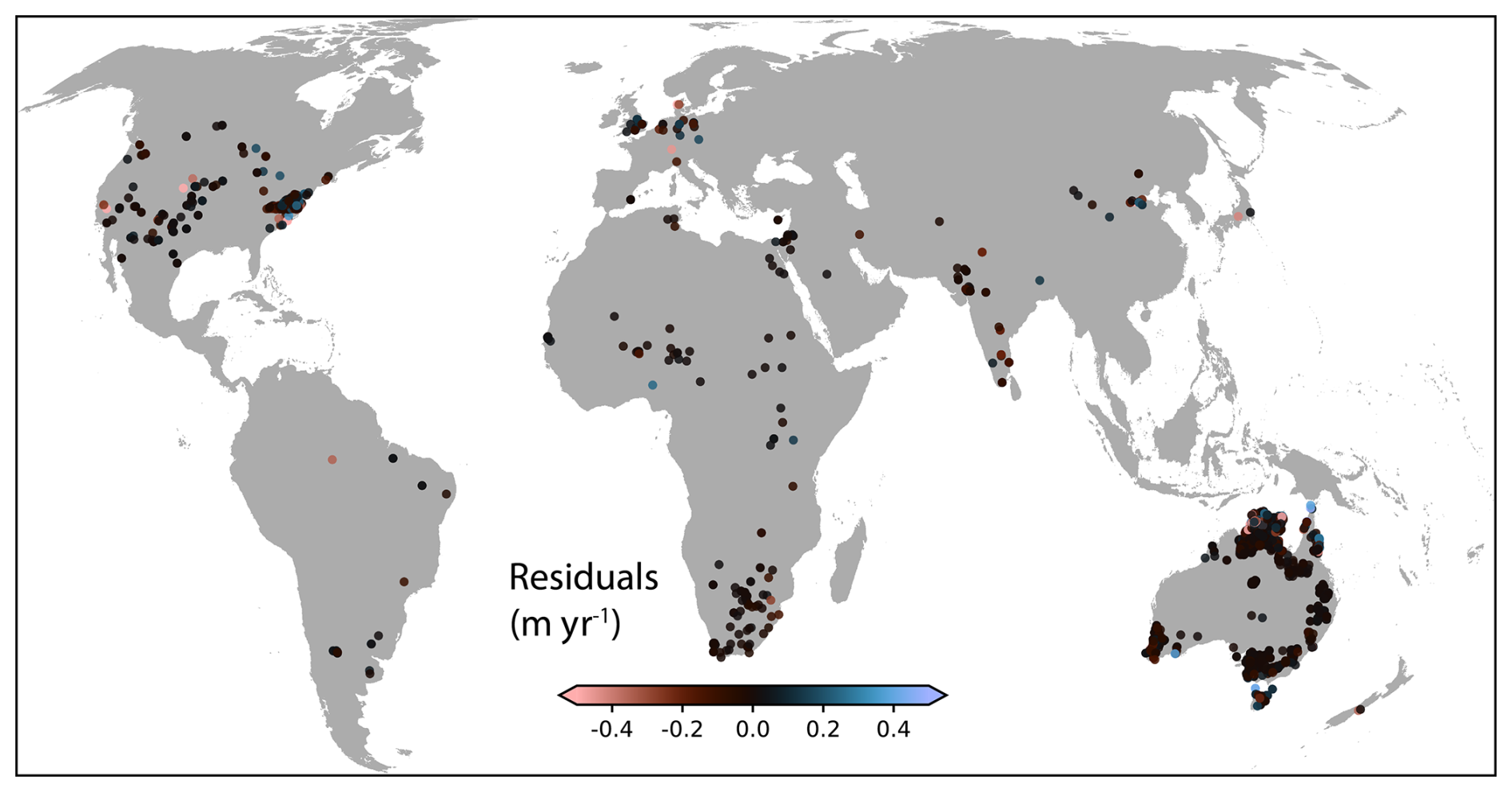
Figure A1 Global distribution of leave-one-out cross-validation residuals for the Generalized Additive Model (GAM) of groundwater recharge.

Appendix B: Derivation of the KGE-NP Mean Flow Benchmark Threshold and Skill Score Normalization

Knoben et al. (2019) define a benchmark as the mean flow simulation, defined as ${\mathrm{Sim}}_{\left(t\right)}=\stackrel{\mathrm{‾}}{\mathrm{Obs}}$ for all time steps t. Under this benchmark, β=1: since ${\mathit{\mu }}_{\mathrm{sim}}=\stackrel{\mathrm{‾}}{\mathrm{Obs}}={\mathit{\mu }}_{\mathrm{obs}}$ by definition, α=0: since the simulated time series is constant, σ_sim=0 and r=0: since a constant series has no temporal variation, the linear correlation with observations is formally undefined; following Knoben et al. (2019), it is assigned a value of zero, as there is no relationship between the fluctuations of the two series. Substituting these values into the standard KGE equation:

$$\begin{array}{}\text{(B1)}& \begin{array}{rl}{\mathrm{KGE}}_{\mathrm{bench}}& =\mathrm{1}-\sqrt{(\mathrm{0}-\mathrm{1}{)}^{\mathrm{2}}+(\mathrm{0}-\mathrm{1}{)}^{\mathrm{2}}+(\mathrm{1}-\mathrm{1}{)}^{\mathrm{2}}}\\ & =\mathrm{1}-\sqrt{\mathrm{2}}\approx -\mathrm{0.41}\end{array}\end{array}$$

Critically, the threshold of −0.41 holds for any observation time series, making it a universal benchmark for the standard KGE. The non-parametric KGE (KGE-NP; Pool et al., 2018) replaces the parametric components of the standard KGE with rank-based and distribution-free analogues:

$$\begin{array}{}\text{(B2)}& \text{KGE-NP}=\mathrm{1}-\sqrt{(r_{\mathrm{s}}-\mathrm{1}{)}^{\mathrm{2}}+({\mathit{\alpha }}_{\mathrm{NP}}-\mathrm{1}{)}^{\mathrm{2}}+(\mathit{\beta }-\mathrm{1}{)}^{\mathrm{2}}}\end{array}$$

where r_s is the Spearman rank correlation between simulated and observed, ${\mathit{\alpha }}_{\mathrm{NP}}=\mathrm{1}-\mathrm{MAE}({\mathrm{FDC}}_{\mathrm{sim}},{\mathrm{FDC}}_{\mathrm{obs}})$ is a non-parametric variability ratio derived from the mean absolute error between the normalized flow duration curves (FDCs) of simulated and observed, and $\mathit{\beta }={\mathit{\mu }}_{\mathrm{sim}}/{\mathit{\mu }}_{\mathrm{obs}}$ is the bias ratio, unchanged from the standard KGE.

Applying the same mean flow benchmark ($\mathrm{Sim}\left(t\right)=\stackrel{\mathrm{‾}}{\mathrm{Obs}}$ for all t) to the KGE-NP formulation: β=1, r=0. However for α_NP the following applies:

$$\begin{array}{}\text{(B3)}& {\displaystyle }{\mathit{\alpha }}_{\mathrm{NP}}& {\displaystyle }=\mathrm{1}-\mathrm{MAE}({\mathrm{FDC}}_{\mathrm{sim}},{\mathrm{FDC}}_{\mathrm{obs}})\text{(B4)}& {\displaystyle }& {\displaystyle }=\mathrm{1}-{\displaystyle \frac{\mathrm{1}}{n\stackrel{\mathrm{‾}}{\mathrm{Obs}}}}\sum _{i=\mathrm{1}}^n\left|{\mathrm{Obs}}_i^{\mathrm{sorted}}-{\stackrel{\mathrm{‾}}{\mathrm{Obs}}}_{\mathrm{obs}}\right|\text{(B5)}& {\displaystyle }& {\displaystyle }=\mathrm{1}-{\displaystyle \frac{{\mathrm{MAD}}_{\mathrm{obs}}}{{\mathit{\mu }}_{\mathrm{obs}}}}\end{array}$$

Substituting all three terms of the mean flow benchmark into the KGE-NP equation:

$$\begin{array}{}\text{(B6)}& \begin{array}{rl}& {\text{KGE-NP}}_{\mathrm{bench}}\\ & =\mathrm{1}-\sqrt{(\mathrm{0}-\mathrm{1}{)}^{\mathrm{2}}+{\left(-{\displaystyle \frac{{\mathrm{MAD}}_{\mathrm{obs}}}{{\mathit{\mu }}_{\mathrm{obs}}}}\right)}^{\mathrm{2}}+(\mathrm{1}-\mathrm{1}{)}^{\mathrm{2}}}\\ & =\mathrm{1}-\sqrt{\mathrm{1}+{\left({\displaystyle \frac{{\mathrm{MAD}}_{\mathrm{obs}}}{{\mathit{\mu }}_{\mathrm{obs}}}}\right)}^{\mathrm{2}}}\end{array}\end{array}$$

Therefore, unlike the standard KGE, the KGE-NP benchmark threshold is not universal since it depends on ${\mathrm{MAD}}_{\mathrm{obs}}/{\mathit{\mu }}_{\mathrm{obs}}$, the coefficient of mean absolute deviation of the observed record. As a result, a single fixed KGE-NP threshold analogous to −0.41 cannot be defined. To recover a universal metric suitable for global-scale evaluation and multi-model comparison, KGE-NP scores were normalized into a skill score following Knoben et al. (2019):

$$\begin{array}{}\text{(B7)}& {\text{KGE-NP}}_{\mathrm{skill}}={\displaystyle \frac{{\text{KGE-NP}}_{\mathrm{model}}-{\text{KGE-NP}}_{\mathrm{bench}}}{\mathrm{1}-{\text{KGE-NP}}_{\mathrm{bench}}}}\end{array}$$

A KGE-NP_skill<0 indicates that a model is worse than the mean flow benchmark, KGE-NP_skill=0 indicates that a model is equal to the mean flow benchmark, and KGE-NP_skill>0 indicates that a model is better than the mean flow benchmark. The benchmark KGE-NP_bench is computed individually for each well from its observed record and places all wells on a common scale, where zero universally denotes the boundary between a model that adds value over the mean flow benchmark and one that does not.

Appendix C: Spatio-temporal Distribution in observations of groundwater head

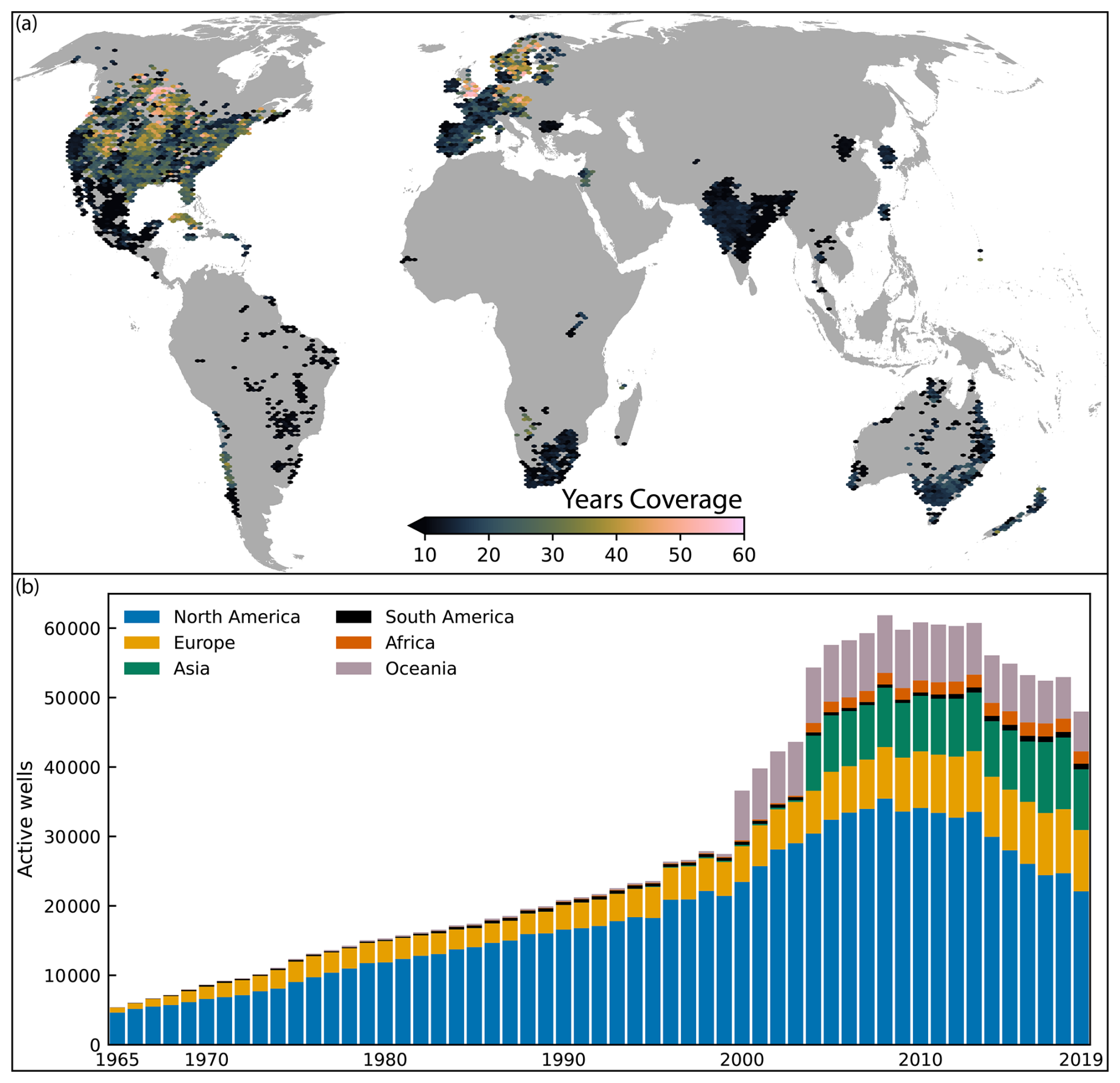
Figure C1 Global distribution and temporal coverage of groundwater observations. (a) Spatial distribution of active groundwater monitoring wells worldwide, colored by the number of years of available data. (b) Number of active groundwater monitoring wells by continent from 1965 to 2019.

Appendix D: KGE-NP_skill Post-hoc Analysis

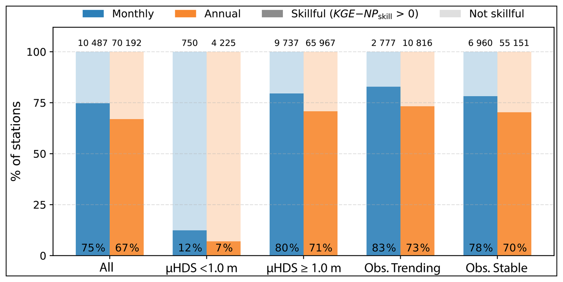
Figure D1 Grouped stacked bar charts showing the percentage of skillful validations, defined as KGE-NP_skill>0. Annotations at the top of each bar indicate the total number of observation wells. The percentages at the bottom of show the proportion of observation wells classified as skillful. Wells are split into trending/stable by thier absolute Theil-Sen slope using a threshold of 0.01 m yr⁻¹. We choose this threshold instead of the 0.1 m yr⁻¹ of Jasechko et al. (2024) because this is more conservative in defining a trends within the stable class.

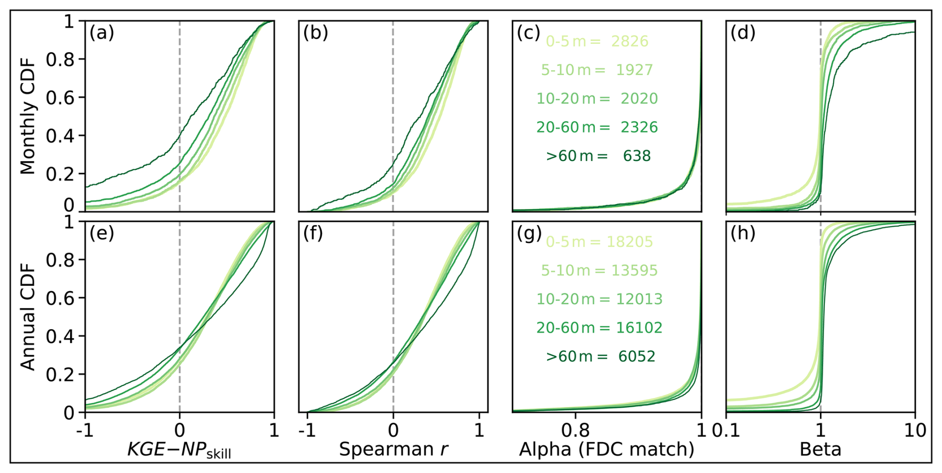
Figure D2 (a, e) KGE-NP_skill CDF filtered for locations where statistical artifacts result in poor performance. Constituent components (b, f) correlation, (c, g) alpha, and (d, h) beta of KGE-NP for monthly and annual groundwater heads simulated by GLOBGM from 1965–2019, grouped by water table depth. Gray lines in panels (a) and (e) symbolize a KGE-NP_skill of 0 which is the threshold at which greater values indicate predictions that improve upon the mean flow benchmark. Gray lines in panels (b) and (f) indicate the point at which correlations are positive to the right and negative to the left. Gray lines in panels (d) and (h) separate over-estimation to the right and underestimation to the left.

Figure D3 (a, e) Boxplots comparing KGE-NP_skill inside and outside quality assurance regions (QA, Sect. 3.2.1) and abstraction regions, for monthly (a–d) and annual (e–h) and its constituent components (b, f) correlation, (c, g) alpha, and (d, h) beta.

Appendix E: GRACE/GRACE-FO Comparison

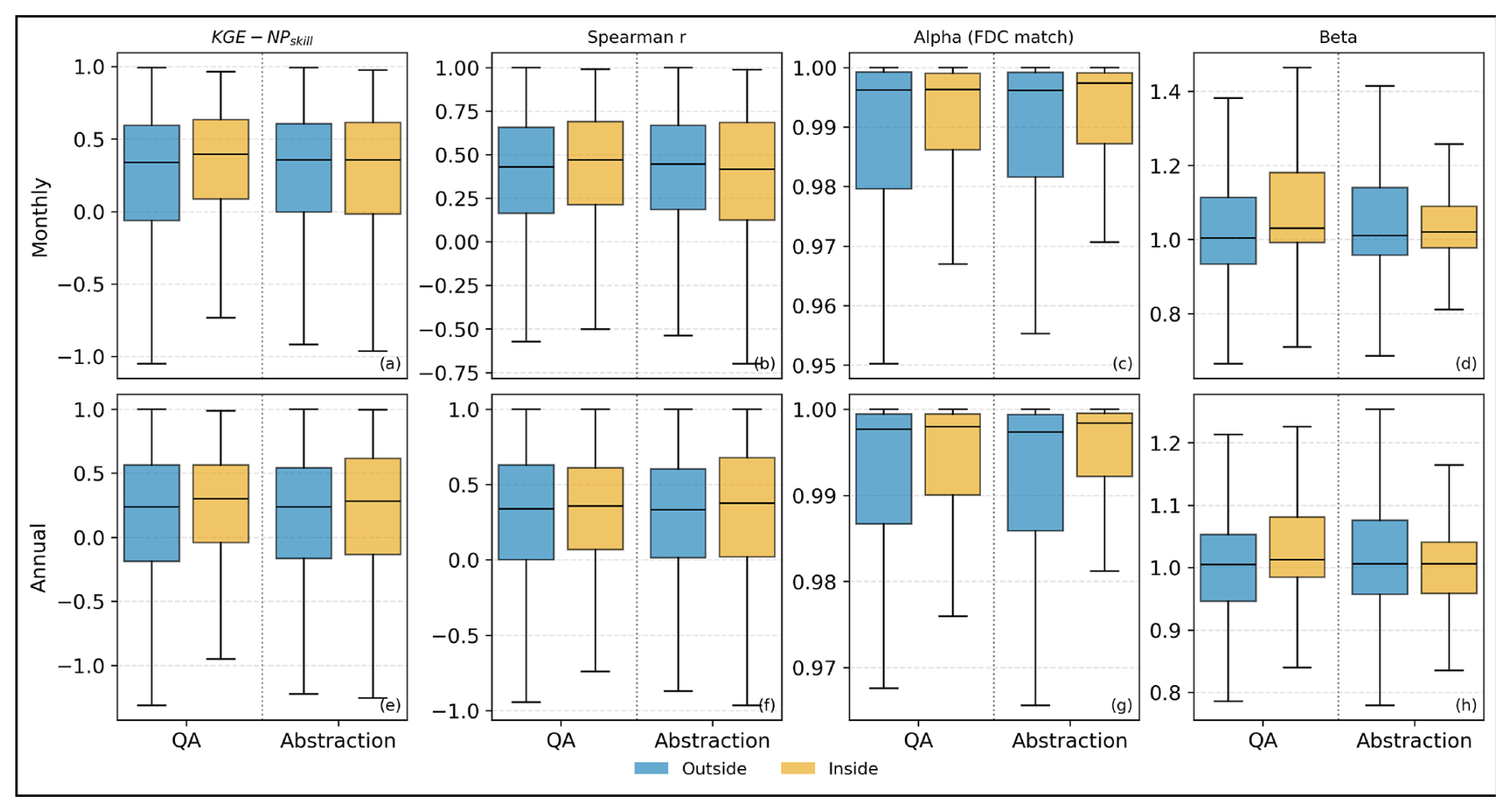
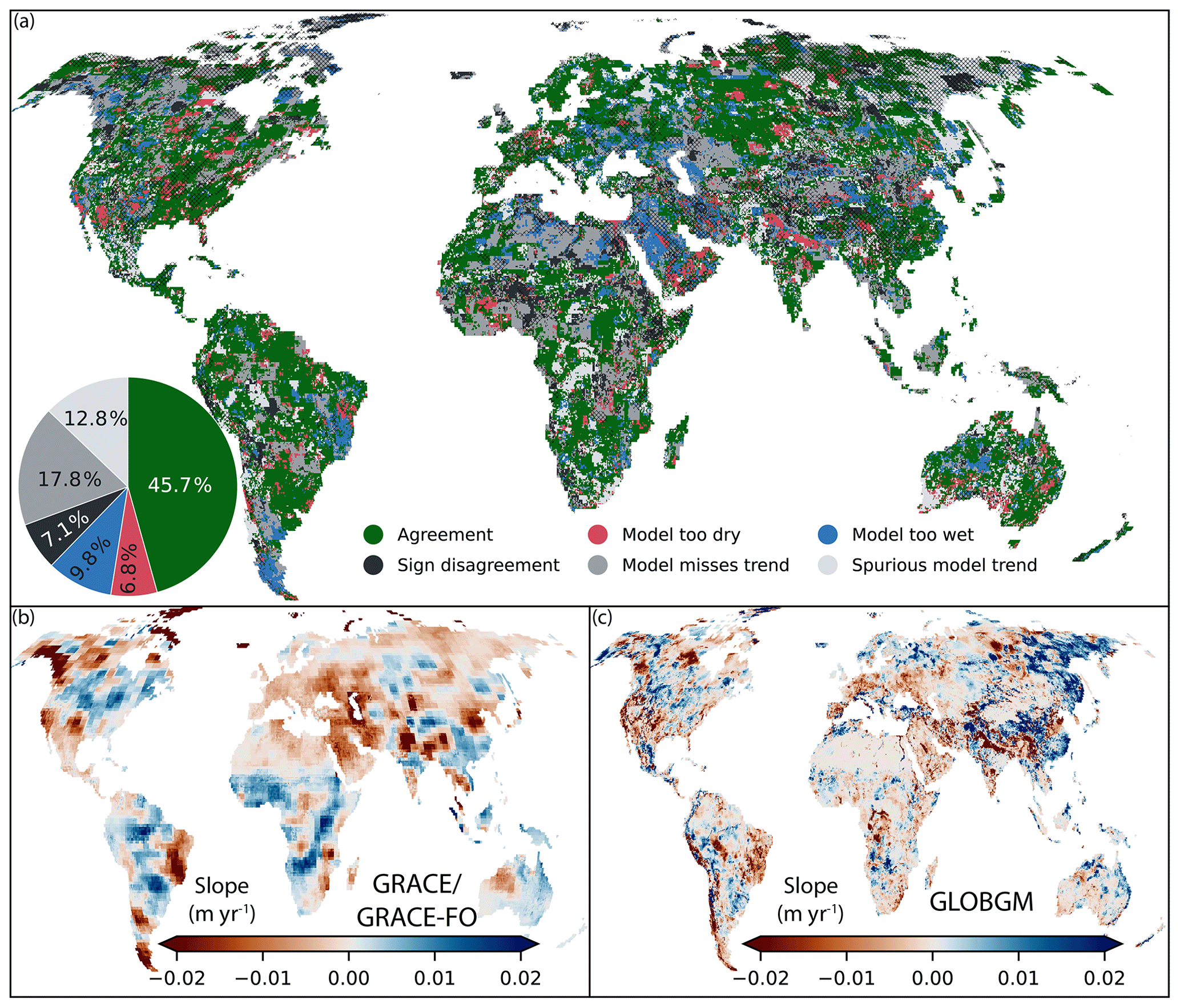
Figure E1 (a) Agreement between GRACE/GRACE-FO and GLOBGM Total Water Storage Anomalies with the inset showing the proportion of land area per agreement class and hatching indicates cells where more than half the underlying 30 arcsec area carries a model quality flag (mountainous terrain, karst, or permafrost). Theil-Sen trends in deseasonalised Total Water Storage Anomalies (2002–2019) from (b) GRACE/GRACE-FO and (c) GLOBGM.

Appendix F: Machine Learning Bias Correction

Table F1 Performance metrics of the two-stage correction ML model for the training, validation, and holdout test sets.

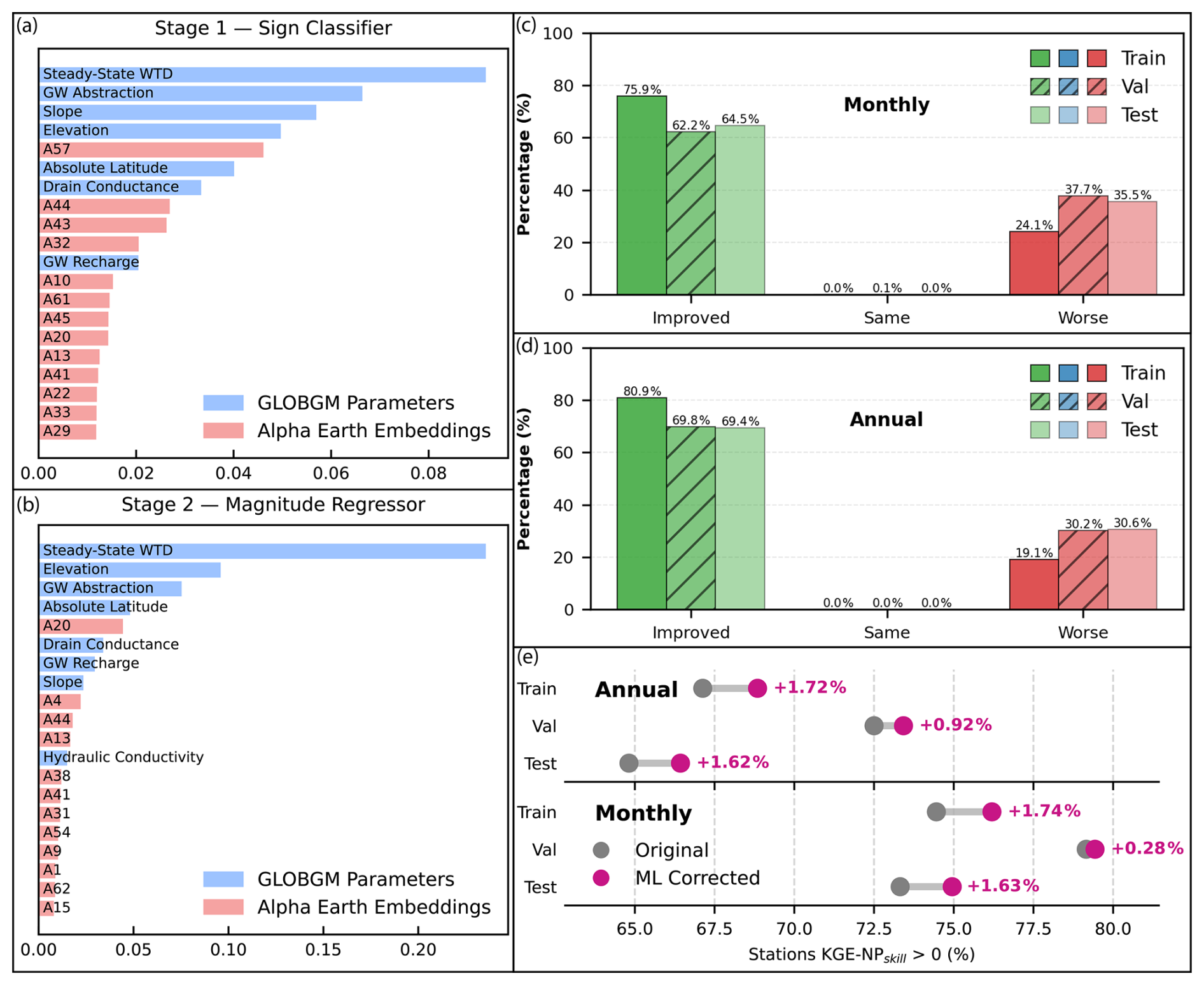
Figure F1 Feature importance of predictors of the (a) binary classifier and (b) magnitude regressor LightGBM models. Percentage of observation wells where bias improved, stayed the same, or worsened at the monthly (c) and annual (d) resolution, separated by train, validation, and test sets. (e) Percentage of observations where KGE-NP_skill>0 before and after bias correction.

Appendix G: Unaggregated Annual Theil-Sen Trends

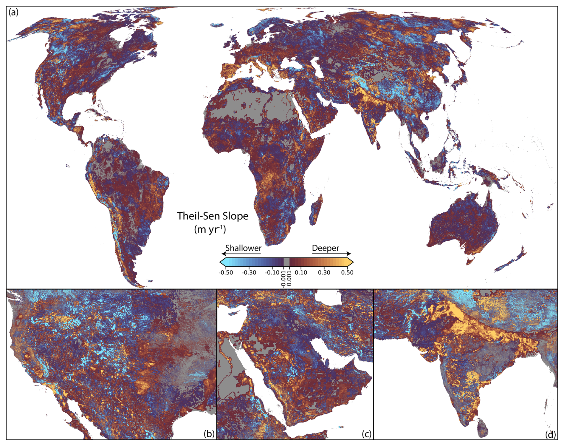
Figure G1 (a) Theil-Sen slope of annual water table depth (1965–2019) simulated by GLOBGM. Gray pixels indicate regions where slopes are either insignificant, less than 0.001 m yr⁻¹, or both. Note that this figure represents the lower model layer which is representative of unconfined and confined aquifers. Zoomed insets provide more detail over (b) United States, (c) the Arabian Peninsula, and (d) the Indo-Gangetic Plain.

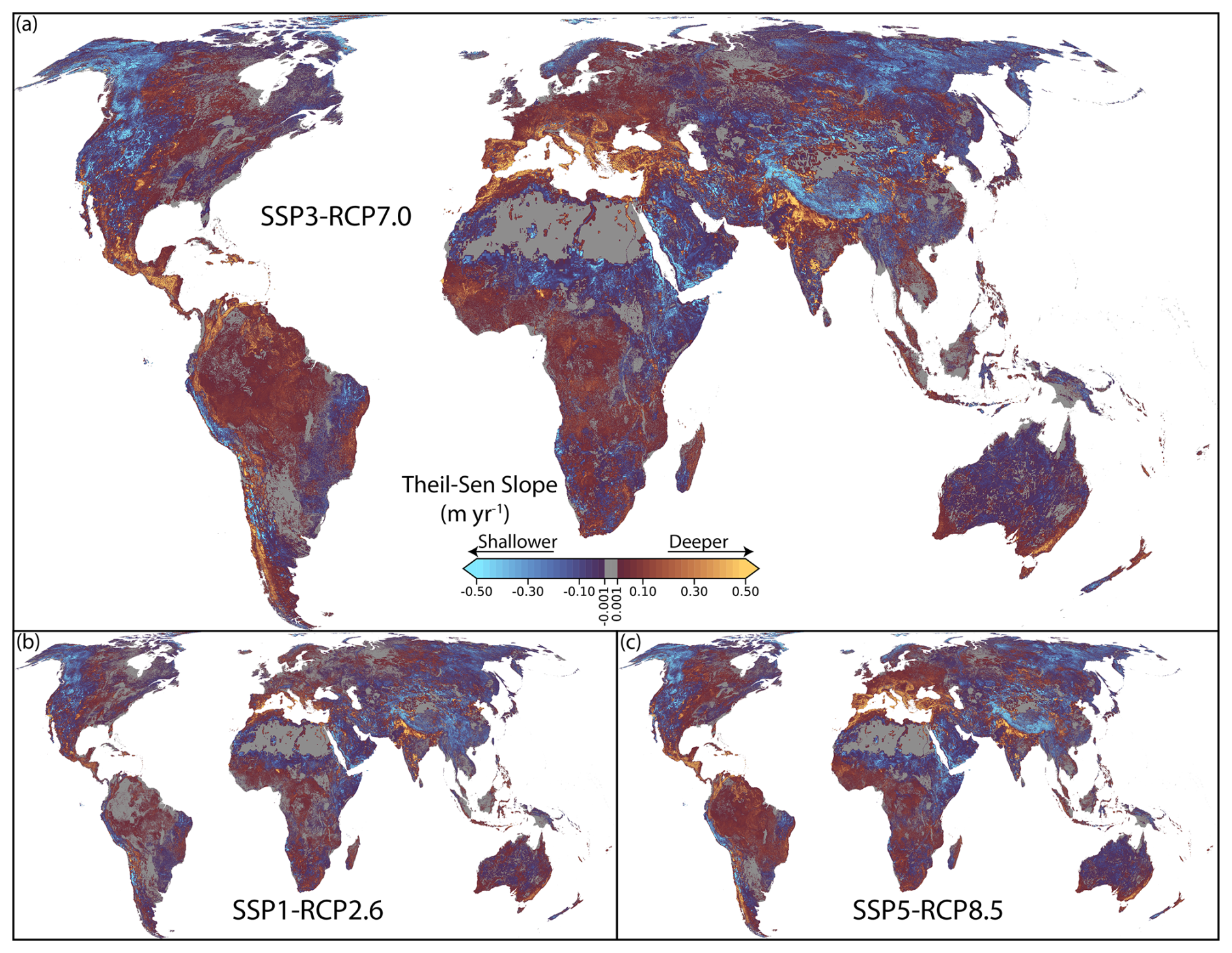
Figure G2 Theil-Sen slope of annual water table depth (2015–2100) simulated by GLOBGM under three SSP-RCP scenarios. Gray pixels indicate regions where slopes are either insignificant, less than 0.001 m yr⁻¹, or both. Note that this figure represents the lower model layer which is representative of unconfined and confined aquifers.