Constraining uncertainty in projected precipitation over land with causal discovery

Accurately projecting future precipitation patterns over land is crucial for understanding climate change and developing effective mitigation and adaptation strategies. However, projections of precipitation changes in state-of-the-art climate models still exhibit considerable uncertainty, in particular over vulnerable and populated land areas. This study aims to address this challenge by introducing a novel methodology for constraining climate model precipitation projections with causal discovery. Our approach involves a multistep procedure that integrates dimension reduction, causal network estimation, causal network evaluation, and a causal weighting scheme which is based on the historical performance (the distance of the causal network of a model to the causal network of a reanalysis dataset) and the interdependence of Coupled Model Intercomparison Project Phase 6 (CMIP6) models (the distance of the causal network of a model to the causal network of other climate models). To uncover the significant causal pathways crucial for understanding dynamical interactions in the climate models and reanalysis datasets, we estimate the time-lagged causal relationships using the Peter–Clark momentary conditional independence (PCMCI) causal discovery algorithm. In the last step, a novel causal weighting scheme is introduced, assigning weights based on the performance and interdependence of the CMIP6 models' causal networks. For the end-of-century period, 2081–2100, our method reduces the very likely ranges (5th–95th percentile) of projected precipitation changes over land between 10 % and 16 % relative to the unweighted ranges across three global warming scenarios (SSP2-4.5, SSP3-7.0, and SSP5-8.5). The sizes of the likely ranges (17th–83rd percentile) are further reduced between 16 % and 41 %. This methodology is not limited to precipitation over land and can be applied to other climate variables, supporting better mitigation and adaptation strategies to tackle climate change.

1 Introduction

Global mean precipitation and evaporation are expected to rise with warming by approximately 2 % °C⁻¹–3 % °C⁻¹, driven by increased atmospheric water vapor according to thermodynamics (Allan et al., 2020). Although recent observations have struggled to detect a response of global precipitation to the current warming level, new research has demonstrated that precipitation variability has already increased globally over the past century (Zhang et al., 2024). The Coupled Model Intercomparison Project Phase 6 (CMIP6) models represent the latest generation of climate models used to simulate past, present, and future climate conditions, providing vital projections to inform policy and adaptation strategies (Eyring et al., 2016). However, a significant challenge associated with these models is the large uncertainty range in land precipitation projections, reflecting the complex nature of precipitation processes and their representation in climate models (Tebaldi et al., 2021). Studies have shown that uncertainty in climate projections can be attributed to multiple factors, including, e.g., model structure, parameterization, and internal variability (Hawkins and Sutton, 2009). Model uncertainty is commonly assessed as the range of values projected by different climate models for a given future scenario (also known as intermodel spread). According to the Intergovernmental Panel on Climate Change (IPCC) Sixth Assessment Report (Douville et al., 2021), the average projected precipitation rate over land increases by 2.4 % in the low-emission scenario by 2081–2100 (with the 17th–83rd percentile range varying from −0.2 % to +4.7 %) relative to the period 1995–2014. In comparison, the very high-emission scenario shows a more substantial increase of 8.3 % (with the 17th–83rd percentile range varying from 0.9 % to 12.9 %) by 2081–2100. Reducing intermodel spread in precipitation projections is crucial for enhancing the reliability of climate projections.

These changes in future precipitation patterns have profound implications for various sectors, including natural and human systems (IPCC; Seneviratne et al., 2021). Kotz et al. (2022) discuss the extensive economic impacts associated with precipitation shifts, emphasizing the need for precise and reliable projections. The economic consequences of climate change, particularly in regions vulnerable to precipitation changes, underscore the urgency of reducing the uncertainty in these projections. Accurate projections are therefore critical for developing effective adaptation and mitigation strategies to minimize these negative impacts and enhance resilience.

To reduce the intermodel spread of future climate projections, a common method is the usage of an emergent constraint (Hall and Qu, 2006; Eyring et al., 2019). An emergent constraint identifies a statistically significant relationship between a constrained observable and a future climate variable. This observable can be a trend or variation observed during the historical period and includes metrics such as temperature variability (Cox et al., 2018) and shortwave low-cloud feedback (Qu et al., 2018). The future climate variable often relates to key climate sensitivity metrics such as equilibrium climate sensitivity (ECS) and transient climate response (TCR) (Nijsse et al., 2020; Schlund et al., 2020b). By establishing a robust statistical relationship and combining it with observed data, the probability distribution of ECS and TCR can be constrained, leading to a narrower range in future climate projections.

However, when it comes to global precipitation and precipitation over land, the emergent constraints tend to be weaker compared to those for TCR or ECS (Ferguglia et al., 2023). Previous studies attribute this to the complexity of precipitation processes, model parameterizations, and observational constraints (Ferguglia et al., 2023). For example, complex atmospheric processes affecting precipitation, including aerosol impacts on cloud microphysics (Allen and Ingram, 2002; Beydoun and Hoose, 2019), convection, and large-scale circulation, are challenging to model accurately, leading to larger uncertainties. Furthermore, climate models use different parameterizations for subgrid-scale processes such as cloud formation, contributing to the spread. In addition, precipitation observations are often limited and carry substantial uncertainties (Trenberth and Zhang, 2018), weakening the relationships between historical predictors and future projections. The robustness of emergent constraints also depends on the specific ensemble of models used. For example, the constraints identified in the previous generation of models, CMIP5, may not hold in CMIP6 (Pendergrass, 2020; Schlund et al., 2020b). Building on this understanding, Shiogama et al. (2022) investigated emergent constraints related to future global precipitation changes using past temperature and precipitation trends. They revised the upper bound (95th percentile) of global precipitation change for 2051–2100 under a medium-greenhouse-gas-concentration scenario from a 6.2 % change to a range of 5.2 %–5.7 %. Additionally, other studies have also explored constraining future precipitation projections using observational data and past warming trends. Thackeray et al. (2022) developed an emergent constraint to reduce the uncertainty in projections of future heavy-rainfall occurrence. Dai et al. (2024) proposed an emergent constraint that utilizes past observational warming trends to constrain future projections of mean and extreme precipitation on both global and regional scales. They constrained the projected globally averaged mean precipitation fractional changes under the high-emission scenario for the 2081–2100 period relative to 1981–2014, reducing the average estimate from 6.9 % to 5.2 % and narrowing the 5 %–95 % range from 3.0 %–10.9 % to 1.9 %–8.5 %.

Other methods have been developed to constrain future climate projections. For instance, Schlund et al. (2020a) employed a machine learning regression approach known as a gradient-boosted regression tree (GBRT) on historical climate data to reduce the uncertainty range of future projections of gross primary production (GPP). Another key method to address the intermodel spread is multimodel weighting based on model performance and interdependence. This addresses the issues in the commonly used “model democracy” approach, used in the IPCC Sixth Assessment Report (IPCC; Lee et al., 2021), where each climate model is given equal weight regardless of its performance and interdependence with other models. Equal weighting can lead to significant issues, such as overrepresenting similar models and ignoring differences in model performance (IPCC; Doblas-Reyes et al., 2021). The methodology introduced by Knutti et al. (2017) and further explored by Brunner et al. (2020) evaluates the historical model performance and interdependence based on several diagnostics and applies weights to combine the model outputs. This technique refines ensemble projections by prioritizing models that more accurately simulate historical climate conditions and accounts for redundancy among models.

These previous studies highlight the importance of using advanced statistical techniques and observational data. Notably, Nowack et al. (2020) introduced a causal model evaluation framework which assesses models based on their ability to capture cause-and-effect relationships within the system. In particular, Nowack et al. (2020) applied a causal discovery algorithm to sea level pressure (SLP) data from CMIP5 simulations and meteorological reanalyses. They constructed causal networks, referred to as fingerprints, to conduct a process-oriented evaluation of the models. Interestingly, models with fingerprints closer to observations better reproduced precipitation patterns over various regions, including South Asia, Africa, East Asia, Europe, and North America. These findings highlight the potential of causal model evaluation to address uncertainties in climate projections but have not yet been applied as such.

Nowack et al. (2020) also underscore the role of using SLP components as proxies for modes of variability to better understand precipitation patterns. Furthermore, we emphasize the strong connection between dynamical interactions imprinted in SLP fields and precipitation patterns. Numerous studies (e.g., Lavers et al., 2013; Thompson and Green, 2004; Müller-Plath et al., 2022) revealed how large-scale pressure variations, such as the North Atlantic Oscillation (NAO), the Azores High, the Arctic Oscillation, and the North Sea–Caspian Pattern, can influence precipitation variability across Europe and the Mediterranean basin. Dia-Diop et al. (2021) have shown that SLP anomalies over specific areas such as the Azores and St. Helena highs are interconnected with monthly mean precipitation in West Africa, indicating a relationship between SLP and rainfall. Furthermore, Benestad et al. (2007) demonstrated the importance of statistical models that use SLP to predict interannual variations in rainfall, revealing the connection between these variables. Costa-Cabral et al. (2016) confirmed the importance of large-scale climate indices, particularly the North Pacific High (NPH) wintertime anomaly, in predicting precipitation variability in northern California. These studies support the broader applicability of SLP indices to understand precipitation patterns.

A research gap lies in the need to explore new methods, such as causal model evaluation, to more accurately assess the performance of climate models. Combining these advanced evaluation techniques with multimodel weighting schemes promises to reduce the uncertainty in climate projections. The goal of this study is to explore causal discovery for evaluating climate models and reducing the uncertainty in their projections, particularly for precipitation over land. We further demonstrate the application of causal approaches in capturing complex climate dynamics. Additionally, we address the practical challenges of integrating causal model evaluation with multimodel weighting. As such, this research will ultimately help to improve projections of precipitation change over land, enhancing our ability to anticipate and respond to the consequences of climate change in populated and vulnerable areas. This is essential for water resource management, agriculture, infrastructure planning, and overall climate resilience efforts (IPCC, 2021).

To constrain precipitation change projections over land, our methodology involves a multistep process that integrates data preprocessing, dimension reduction, causal relationship estimation, causal network evaluation, and model weighting. Our study utilizes CMIP6 historical simulations of sea level pressure (SLP) complemented by reanalysis datasets which serve as references. Future projections based on shared socioeconomic pathways (SSPs; O'Neill et al., 2014) are employed to calibrate the weighting scheme and project precipitation changes. To address the high dimensionality of the data, principal component analysis (PCA; Shaffer, 2002; Ramsay and Silverman, 2005) with varimax rotation (Rohe and Zeng, 2023; Kaiser, 1958) is utilized, extracting 60 components that capture the essential modes of variability. We estimate the time-lagged causal relationships using the PCMCI (Peter–Clark momentary conditional independence; Runge et al., 2019b) causal discovery algorithm to uncover the significant causal pathways crucial for understanding dynamical interactions in the climate models. The identified causal networks are evaluated against the reference networks derived from the reanalysis data using the F₁ score and its complement 1−F₁. The causal networks of the climate models are also compared with one another with the F₁ score to measure their similarities. This quantitative approach provides insights into the relative performance and uniqueness of each model's representation of dynamical processes. In the last step, a novel causal weighting scheme is introduced, assigning weights based on the performance and interdependence metrics of the causal networks. This scheme prioritizes models closely matching the reference causal network and exhibiting distinctive causal structures. The resulting weights inform the computation of the multimodel-weighted means and ranges of precipitation changes over land.

Section 2 provides an overview of the materials and methods used in this study. The results are detailed in Sect. 3. We summarize and discuss our findings in Sect. 4.

2 Materials and methods

Here we introduce the data and methodology used in this study. Section 2.1 describes the CMIP6 and reanalysis data that we integrate. Section 2.2 explains the preprocessing of the data and its relevance in this study. Section 2.3–2.6, respectively, introduce our multistep methodology consisting of dimension reduction, causal network estimation, causal network evaluation, and causal weighting of climate models. Figure 1 presents the different steps of our framework.

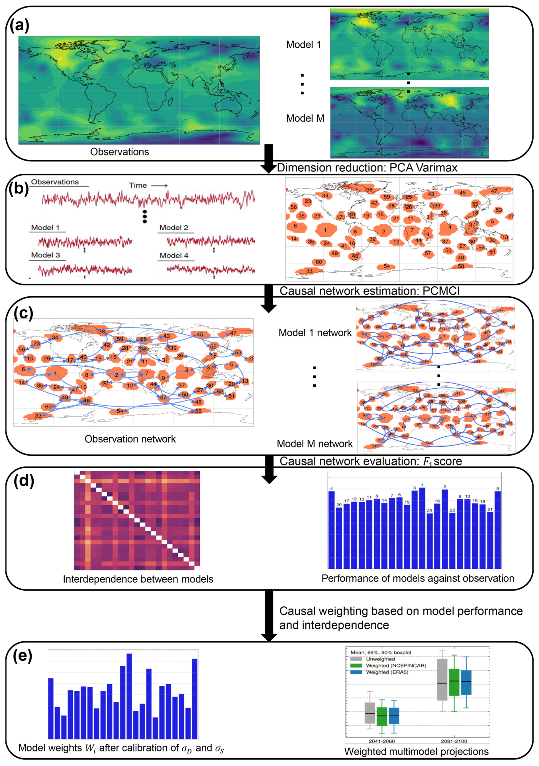
Figure 1 Overview of the causal weighting framework. (a) Daily SLP data from NCEP–NCAR and ERA5 reanalyses are reduced using PCA–varimax to yield (b) regionally confined climate modes for each meteorological season and climate model. PCMCI estimates lagged causal relationships, resulting in (c) dataset-specific causal networks for reanalysis and climate models. These networks enable (d) causal model evaluation via network similarity and (e) causal model weighting, which informs the multimodel-weighted precipitation projections over land.

2.1 Data

This study utilizes CMIP6 historical simulations of SLP spanning 1979 to 2014, with daily time resolution. These simulations, derived from 23 different climate models, each with 2 to 10 ensemble members, are used to estimate the historical causal networks. This results in a total of 154 ensemble members. The daily resolution of the SLP data provides a robust foundation for analyzing the climate models and evaluating their performance in simulating SLP patterns. In addition to the historical simulations of CMIP6, the study employs ERA5 reanalysis datasets (Hersbach et al., 2020) and NCEP–NCAR (Kalnay et al., 1996), covering the period 1979–2014 with daily resolution. These reanalysis datasets serve as a reference for estimating the causal networks of SLP, providing a benchmark against which the performance of the climate models could be assessed. In addition to the SLP datasets, future climate projections of precipitation of the same climate models are incorporated using simulations based on three shared socioeconomic pathways (SSPs; O'Neill et al., 2014) – the medium-emission SSP2-4.5 scenario (101 total members), the high-emission SSP3-7.0 scenario (96 total members), and the very high-emission SSP5-8.5 scenario (107 total members) – for the period 2015–2100, focusing on precipitation over land with yearly time resolution. These simulations are used to calibrate the model performance parameter σ_D of the weighting scheme. They are also used for the projections of precipitation changes over land. A complete list of included models and members for the SLP historical simulations and precipitation SSP simulations is available in Table S1 in the Supplement.

2.2 Data preprocessing

The preprocessing of the SLP data involved several crucial steps to ensure consistency and enhance the quality of the analysis. Firstly, all datasets (including the ERA5 dataset) are linearly interpolated to the 2.5° latitude × 2.5° longitude grid of NCEP–NCAR. Subsequently, the daily data are detrended on a grid-cell basis to remove small trends and ensure robust causal discovery. Anomalies are then calculated using a long-term daily climatology by subtracting each day's mean and dividing by its standard deviation. While SLP data are largely stationary even under historical forcing (Nowack et al., 2020), these steps improve the stationarity of the time series, which is essential for the effective application of the PCMCI causal discovery algorithm (Runge et al., 2023a). Additionally, the data are separated to isolate winter (DJF: December, January, February), spring (MAM: March, April, May), summer (JJA: June, July, August), and autumn (SON: September, October, November), as different causal dependencies are expected for each meteorological season.

2.3 Dimension reduction (Step 1)

As in Nowack et al. (2020), a PCA with varimax rotation is used to extract the main modes of variability and to manage the high dimensionality of the SLP dataset. This dimension reduction step is crucial to represent the processes of interest.

PCA serves as a dimension reduction technique, preserving as much information as possible while reducing the number of dimensions (Shaffer, 2002; Ramsay and Silverman, 2005). This is accomplished by identifying orthogonal linear combinations (known as principal components) from the original spatial data. These initial components often lack straightforward interpretation. Varimax rotation's role is to enhance interpretability by transforming the principal components. Varimax rotation achieves this by maximizing the variance of loadings on each component (Rohe and Zeng, 2023; Kaiser, 1958). The loadings become more localized on specific variables, making them distinct and easier to interpret.

The PCA–varimax transformation is derived from the reference reanalysis datasets individually for each season and subsequently applied to the datasets of all climate models. For the final analysis, the first 60 components are selected that capture the essential characteristics of the variability in SLP data. In the remainder of the study, we use the terms components and modes interchangeably to refer to the PCA–varimax components.

2.4 Causal network estimation (Step 2)

The next step is the estimation of time-lagged causal relationships within the reduced datasets. As correlation alone does not establish causation, we choose to apply causal discovery methods, which come with certain assumptions. Here, the assumptions are that all the relevant variables are included in the analysis (causal sufficiency), the causal relationships and the distributions of the variables remain consistent in the sample data (stationarity), and the statistical dependencies and independencies are a true reflection of the underlying causal structure (faithfulness and Markov condition) (Runge et al., 2023a). We underscore that not all of these assumptions are strictly verified in this study. For instance, causal sufficiency is not fully met, as our analysis is restricted to SLP causal networks. However, these assumptions are less critical in our case because our main goal is to derive a metric of the data rather than to determine the exact causal relevance of each link. The rationale behind using causal discovery is that it offers a more precise estimation of dynamical interactions compared to correlation networks, thanks to its ability to filter out spurious relationships.

Given this last assumption, we choose to implement the PCMCI causal discovery algorithm, which is well suited for time series data with no contemporaneous effects (Runge et al., 2019b). PCMCI aims to uncover causal relationships among variables by assessing conditional dependencies over different time lags. PCMCI builds on the PC algorithm – a constraint-based causal discovery method – by incorporating momentary conditional independence (MCI) tests. These tests help identify causal links even when variables exhibit high autocorrelations, which is common with climate time series (Runge et al., 2019a). During the MCI step, the PCMCI algorithm tests for conditional independence among variables. A causal link is only considered significant if the p value of the test is less than or equal to a significance level α_MCI set by the user.

In this study, the PCMCI algorithm is applied to the principal component time series of each dataset (one dataset per member and season), which are derived from the previous dimension reduction step. The PCMCI algorithm outputs a causal network, enabling the identification of causal pathways between the SLP modes of individual climate datasets or reanalysis datasets. This step identifies significant causal relationships, which is crucial for understanding the dynamical interactions between the SLP modes.

2.5 Causal network evaluation (Step 3)

Following the identification of causal relationships, the resulting causal networks are evaluated using similarity and distance metrics. Given the relatively large size, consisting of 60 variables and a maximum time lag of 20 d, it is challenging to discern patterns. This complexity underscores the necessity of employing a similarity metric to facilitate the comparison of causal networks. The similarity is quantified using the F₁ score introduced in Nowack et al. (2020), while its complement 1−F₁ score serves as a measure of distance. The F₁ score is defined as the harmonic mean between precision and recall, where $\text{precision}=\frac{\text{TP}}{\text{TP}+\text{FP}},\text{recall}=\frac{\text{TP}}{\text{TP}+\text{FN}}$ and $F_{\mathrm{1}}=\frac{\mathrm{2}\cdot \text{precision}\cdot \text{recall}}{\text{precision}+\text{recall}}$.

Compared to a reference network, FP represents the count of falsely identified links, FN is the count of undetected links, and TP denotes the number of correctly identified links. Like Nowack et al. (2020), we adjusted the traditional F₁ score definition to account for the sign of the dependencies and integrated a relaxation of the time lags of identified links. Specifically, if a link exists in reference network A and corresponds to a link in network B with the same causal direction within a time range of ±τ_Diff time lags, we consider it a correctly identified link (TP).

The performance of each climate model's causal network is assessed against a reference causal network derived from observational data, with the distance to this reference network serving as the performance metric. Furthermore, the interdependence among the causal networks of the climate models is quantified, reflecting the degree of similarity or divergence among the networks. Smaller distance values indicate greater similarity, in terms of both performance relative to the reference and dependence among the models. These measures are averaged over separate causal networks obtained for the four meteorological seasons for each model and reanalysis dataset. The results provide insights into the relative performance and distinctiveness of each model's representation of atmospheric dynamical processes.

2.6 Causal weighting scheme based on performance and interdependence (Step 4)

In this study, we develop a new weighting scheme called causal weighting, which is based on the performance and interdependence of the model causal networks. Specifically, we measure performance and assess interdependence between the networks using the complements of the F₁ scores, calculated as 1−F₁ score. These scores are then normalized by the median score across all models. The causal weighting scheme aims to assign higher weights to models that closely match the reference causal network (indicating high performance) and exhibit unique causal structures (indicating high independence). The scheme is formulated as

$$\begin{array}{}\text{(1)}& {\displaystyle }{\displaystyle }{w}_i\propto {\displaystyle \frac{{\mathrm{e}}^{\frac{-{\left(\mathrm{1}-F_{\mathrm{1}}^i\right)}^{\mathrm{2}}}{{\mathit{\sigma }}_D^{\mathrm{2}}}}}{\mathrm{1}+{\sum }_{j\ne i}^M{\mathrm{e}}^{\frac{-{\left(\mathrm{1}-F_{\mathrm{1}}^{ij}\right)}^{\mathrm{2}}}{{\mathit{\sigma }}_S^{\mathrm{2}}}}}}.\end{array}$$

In Eq. (1), M indicates the number of models in the ensemble, $\mathrm{1}-F_{\mathrm{1}}^i$ is the normalized “distance” of model i relative to observations or reanalyses, and $\mathrm{1}-F_{\mathrm{1}}^{ij}$ is the normalized “distance” of model i relative to model j. Weights are normalized to sum to 1. The causal weighting is inspired by the scheme introduced in Knutti et al. (2017) and further explored in several follow-up studies (Brunner et al., 2020). In the original scheme, the performance and interdependence are measured with root-mean-square differences (RMSDs).

The parameters σ_D and σ_S determine the balance between model performance and interdependence. The calibration of the interdependence shape parameter σ_S is performed first. In the original weighting scheme, different options are available to calibrate σ_S as reported in Merrifield et al. (2020). We choose one of the more robust options. Namely, we identify an interdependence shape parameter larger than the typical distances between members of the same model but smaller than the typical intermodel distances. More independent models are given smaller denominators, resulting in larger weights.

The other weighting parameter is the performance shape parameter σ_D. Large σ_D values result in equal weighting across models, whereas small σ_D values cause aggressive weighting, with high-performance models receiving the majority of the weights. After calibrating σ_S, a perfect model test is used to estimate the performance shape parameter σ_D by evaluating climate models based on their historical performance without being overconfident (Karpechko et al., 2013; Abramowitz and Bishop, 2015; Wenzel et al., 2016; Sanderson et al., 2017; Knutti et al., 2017; Brunner et al., 2020). In the perfect model test approach, each model is sequentially treated as the “truth”, while the other models are weighted to project the future target response of the perfect model. After testing σ_D values between 0.1 and 2.0, the calibration selects the smallest σ_D value for which the projection is not overconfident, i.e., when 80 % of these “perfect models” fall within the 10th–90th percentile range of the weighted distribution in the target period. To prioritize performance over interdependence in the weighting trade-off, we reduce this proportion to 70 %. In this study, the target to predict is the precipitation over land for different SSPs and periods (2041–2060 and 2081–2100), resulting in different calibrated values.

Once the two shape parameters have been calibrated, the weights are computed to obtain multimodel-weighted means and ranges of future climate projections. The weighting scheme and associated figures were developed using the Earth System Model Evaluation Tool (ESMValTool) version 2 (Eyring et al., 2020; Righi et al., 2020; Lauer et al., 2020; Brunner et al., 2020; Schlund et al., 2023).

2.7 Technical details

Both the observational data and the climate model simulations contain internal variability, which can introduce noise and potentially bias the comparison between models and observations. To mitigate its influence, multiple ensemble members for each model were processed, with causal networks derived independently for each. The final F₁ scores represent an ensemble average, which reduces the variability effects by smoothing out member-specific results. Recognizing that reanalysis datasets themselves are subject to internal variability and measurement uncertainties, we have analyzed multiple reanalysis products (ERA5 and NCEP–NCAR).

In the dimension reduction step, we keep the first 60 components of the 100 obtained from the PCA–varimax analysis. Some tests are also performed with only the first 50 components. Components with unresolved frequency spectra or dipolar patterns are discarded similarly to the methodology used in Nowack et al. (2020). This selection ensures that only the most significant and stable modes of variability are considered, enhancing the quality of the following steps in our methodology.

Time-lagged dependencies within the data are estimated using the PCMCI algorithm, with a minimum time lag τ_min of 1 d and with a maximum time lag τ_max set to 20 d, though trials with a maximum time lag of 10 d are also tested. PCMCI outputs a time series directed acyclic graph (DAG; Runge et al., 2023a), where the nodes represent variables, the directed edges indicate lagged causal relationships, and there are no cycles in the graph. We assume that the causal dependencies are linear and with additive Gaussian noise. Under such assumptions, we employ the partial correlation conditional independence tests within PCMCI to detect these dependencies. The hyperparameter α_MCI, which controls the significance threshold for the PCMCI algorithm's MCI step, is set to 10⁻⁵ in the results presented in the main text. We briefly investigate the sensitivity of the causal model evaluation to larger values of this parameter in Appendix D1.

The causal network evaluation employs the F₁ score, which is “relaxed” by counting links as true positives even if they occur at slightly different time lags than the reference. We set this window at 2 d (τ_Diff=2 d).

3 Results

In this section, we present the findings for each step of our methodology as applied to the CMIP6 model datasets.

3.1 Dimension reduction and causal network estimation (Steps 1 and 2)

Results of the dimension reduction step are shown in Figs. A1 and A2 in the Appendix. In our analysis, we chose to retain the first 60 components from the 1979–2014 data to better cover the Northern Hemisphere, particularly during the JJA season. Using SLP data from 1948 to 2017, Nowack et al. (2020) truncated and kept a selection of 50 components, discarding additional components due to unphysical time series, such as sudden jumps observed in 1979 when entering the satellite era. We do not encounter these jumps in the time series that start in 1979. We also perform tests with 50 components to investigate the stability of the methodology. Components retrieved from NCEP–NCAR were used across all climate models to obtain reduced datasets. Additionally, components derived from ERA5 were used as an alternative reference for all models.

Discussed in more detail in Appendix B, our findings indicate that the causal network estimation step identifies physically meaningful dependencies between the SLP modes for both reanalysis datasets.

3.2 Causal network evaluation (Step 3)

Figure 2 compares climate models' causal networks' F₁ scores relative to NCEP–NCAR and ERA5 reference datasets. Higher F₁ scores indicate greater similarity between model networks and the references, averaged across all members and seasons. Interestingly, the F₁ scores are consistently higher when compared to ERA5 than to NCEP–NCAR, indicating that the models' dynamical SLP patterns generally match ERA5 more closely. A more detailed analysis of the consistency between the model performance across reanalysis datasets and meteorological seasons is given in Appendix C.

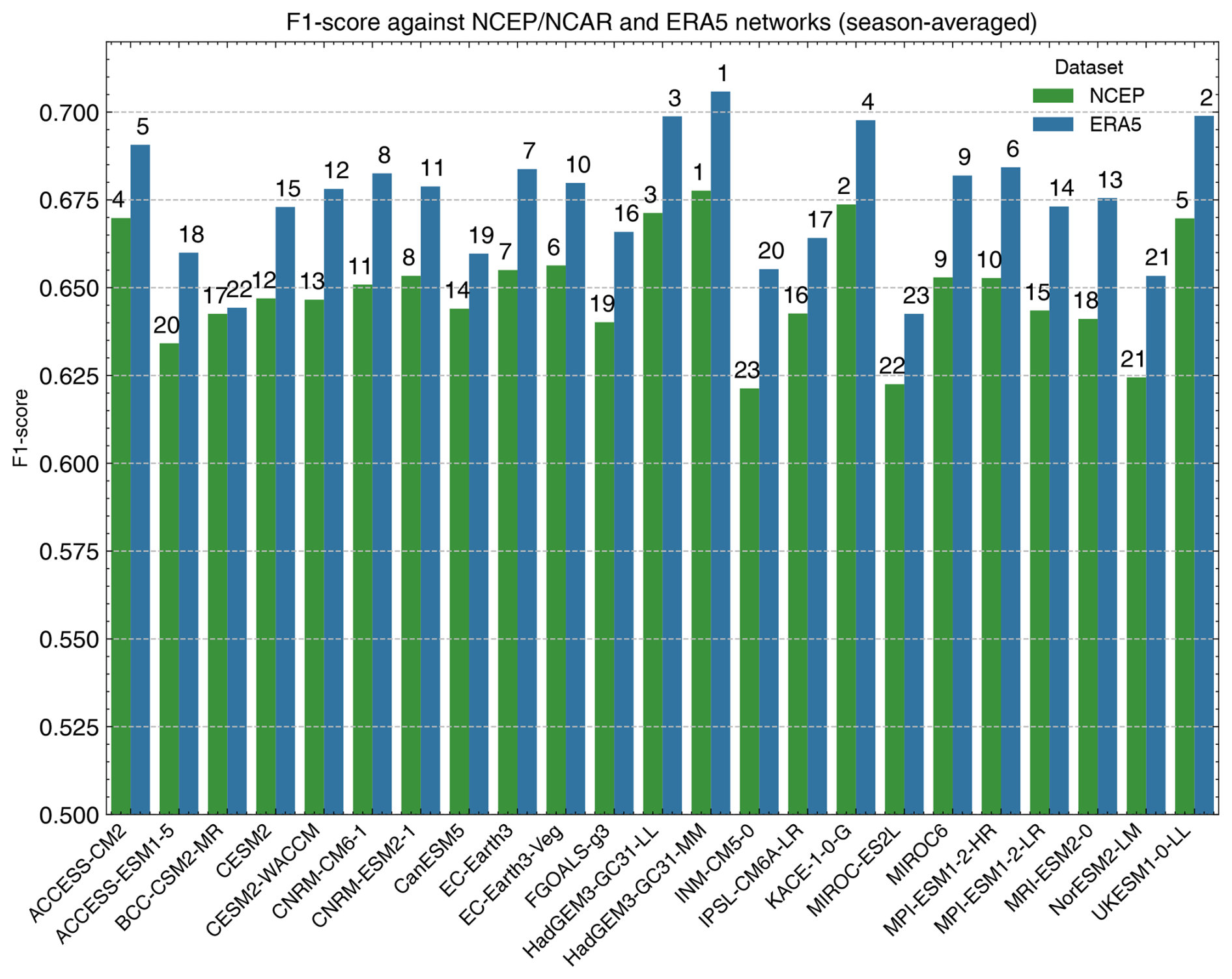
Figure 2 Comparison of the climate models' causal networks' F₁ scores with NCEP–NCAR (green) and ERA5 (blue) as reference. This figure illustrates the similarity between climate models' causal networks and those of the reference reanalysis datasets, averaged across all available members and seasons, using the F₁ score. Higher F₁ scores indicate greater similarity. The rank of each model's similarity is denoted on top of each bar.

Sensitivity tests for the significance level α_MCI, the maximum time lag parameter in PCMCI, and the number of components retained during the dimension reduction step are provided in Appendix D.

In Fig. 3, models with shared developmental features exhibit higher causal network similarity, likely due to their comparable dynamical representations. For example, the ACCESS, UKESM, HadGEM, and K-ACE models share more similar causal networks as measured by the F₁ scores. As reported in the genealogy tree of CMIP6 models in Kuma et al. (2023), the HadGEM2 model was an ancestor of the aforementioned models. Additionally, climate models developed by the same institute (such as the CNRM-CM6-1 and CNRM-ESM2-1) exhibit more similar causal networks, as indicated by the F₁ scores. This finding confirms that the evaluation of the SLP causal networks can identify models with similar physical cores and, consequently, similar dynamical sea level pressure processes. This result is consistent with previous literature, as Nowack et al. (2020) showed that CMIP5 models with shared development and atmospheric models also exhibited more similar causal networks.

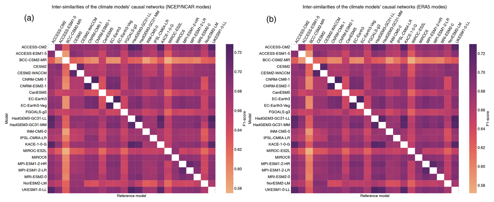
Figure 3 Similarities of the climate models' causal networks when the modes are obtained from (a) NCEP–NCAR and (b) ERA5. This figure illustrates the similarity between the causal networks of different climate models. Similarity is quantified using the F₁ scores between two models. Higher values denote greater similarity or lower independence. The causal networks of one climate model (row) are compared against the causal networks of other climate models used as reference (columns). The values are averaged across the members of each climate model and over all seasons.

Figure 4 shows the relationship between the F₁ scores of the CMIP6 climate models' causal network and the changes in precipitation over land for the SSP2-4.5, SSP3-7.0, and SSP5-8.5 scenarios. The shape indicates an approximately parabolic relationship over the space of opportunities covered by CMIP6 models between the F₁ scores and the precipitation changes. Statistically significant parabolic relationships (polynomial of degree 2) with p values of less than 0.05 (except for a p value of 0.06 for SSP3-7.0 and ERA5 reference) are found. Significant parabolic relationships are found for all SSPs and the two different references, underscoring the robustness of this relationship for different global warming scenarios and reference reanalysis datasets. Notably, climate models with higher F₁ scores, indicating better representations of observed dynamical sea level pressure patterns, tend to cluster around the center of the parabola. These models project precipitation changes in the mid-range compared to other CMIP6 models. In contrast, climate models with lower F₁ scores, indicating lower representations of observed dynamical sea level pressure patterns, tend to either overestimate or underestimate precipitation changes over land. Nowack et al. (2020) previously reported a significant parabolic relationship between precipitation changes under the RCP8.5 scenario and F₁ scores of CMIP5 models. Our findings extend this relationship to CMIP6 models using daily data, compared to the 3 d resolution in Nowack et al. (2020), suggesting that F₁ scores may serve as a robust constraint for projecting precipitation changes over land.

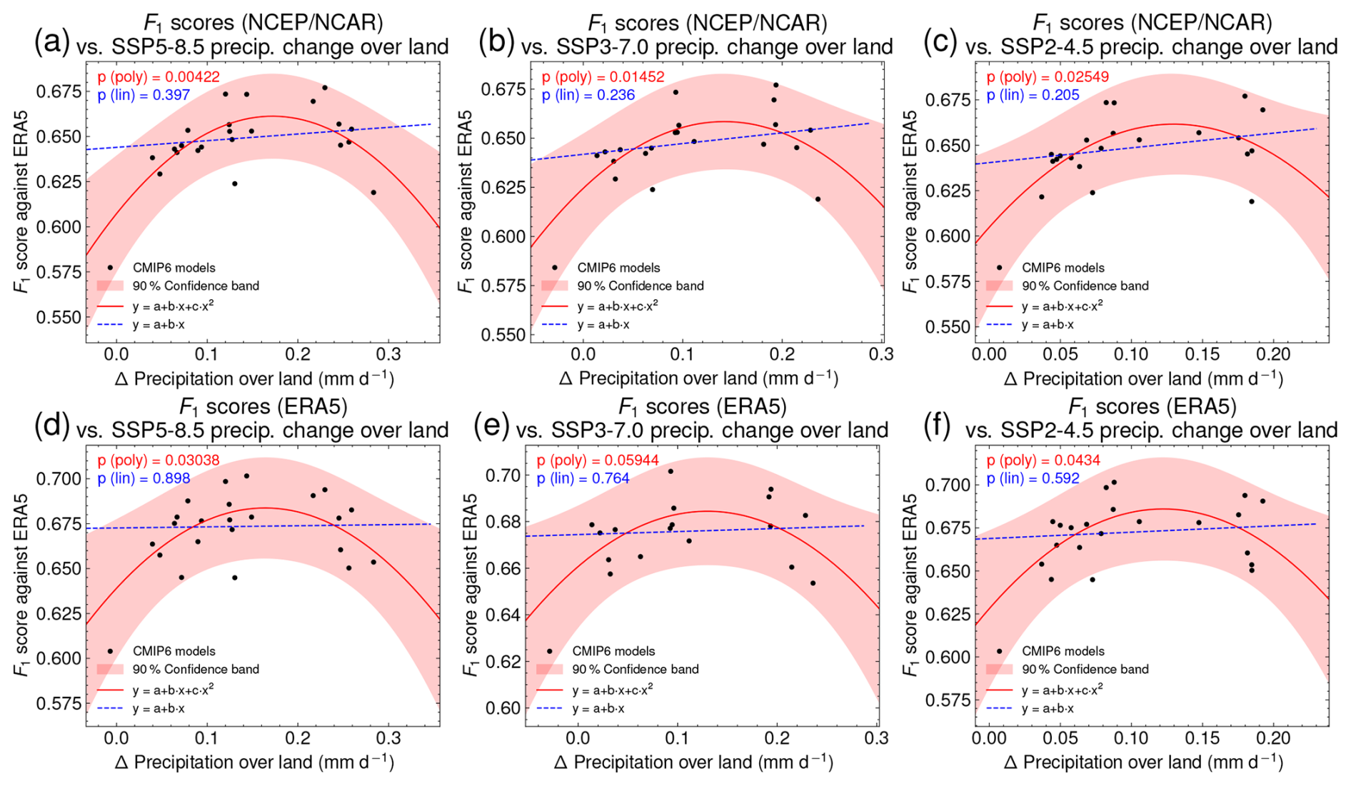
Figure 4 Relationship between precipitation change over land under SSP2-4.5 (c, f), SSP3-7.0 (b, e), and SSP5-8.5 (a, d) scenarios and F₁ scores, using NCEP–NCAR (a–c) and ERA5 (d–f) causal networks as references. The x axis shows precipitation changes between 1850–1900 and 2050–2099, while the y axis represents F₁ scores of climate model causal networks relative to the reference. F₁ scores are averaged across all seasons and available members of a model. The solid red line shows a polynomial fit, and the red-filled area depicts the 90 % confidence band based on a two-tailed t test. The dashed blue line corresponds to the linear fit.

Unlike emergent constraints, which typically display linear relationships, we present a different approach. On the x axis in Fig. 4, we consider a metric which is an observable (the causal network) relative to the observed values (the reference causal network), rather than the observable itself. As a result, the relationship is not linear but rather a concave function with a peak, here an approximately parabolic relationship between the F₁ scores and the precipitation changes.

3.3 Causal weighting scheme based on performance and interdependence (Step 4)

Our previous findings suggest that leveraging the climate models' causal networks' similarity to reference reanalysis causal networks and the intermodel similarities can be promising to constrain precipitation changes over land. We found that models sharing atmospheric characteristics exhibit higher causal network similarity, highlighting the ability of the methodology in capturing sea level pressure (SLP) dynamics accurately. Furthermore, the parabolic relationship between F₁ scores – measuring a model's ability to replicate observed SLP dynamics – and its projection of precipitation changes over land support the use of the F₁ scores as a diagnostic to weight climate projections of precipitation based on their SLP representation skill.

Using the notation of Eq. (1), the complement of the F₁ score serves to measure the distance of models to a chosen reference reanalysis dataset and to evaluate the interdependence among the different models. These distances are separately normalized by the median over all models. After this normalization, the distances can range from 0 to values greater than 1.

The interdependence shape parameter σ_S is calibrated first. We calculate the average distance between members of the same model and the average distance between members of different models. A robust choice for σ_S should lie between these typical distances. These distances are presented in Fig. E1, leading to a calibrated σ_S value of 0.9.

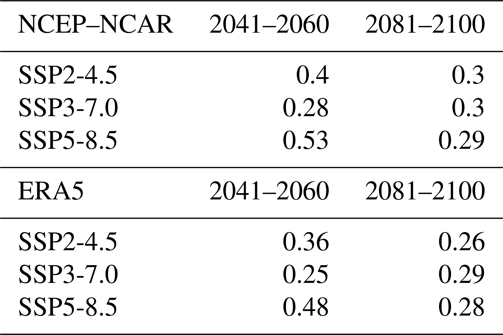
The model performance parameter σ_D is then calibrated using the perfect model test described in Sect. 2.6. A specific σ_D value was calibrated for each SSP (SSP5-8.5, SSP3-7.0, SSP2-4.5), target period (2041–2060 and 2081–2100), and reference dataset (NCEP–NCAR and ERA5). The calibration results, reported in Table 1, range from 0.25 to 0.53.

Table 1 Calibrated performance shape parameters σ_D for different target periods (columns), SSPs (rows), and reference reanalysis datasets (sub-tables).

3.4 Weighted projections of land precipitation changes

Using the calibrated shape parameters, the weights for each combination of SSP, target period, and reference dataset are derived by applying Eq. (1). These weights are used to calculate the weighted projections for a medium- (SSP2-4.5), high- (SSP3-7.0), and very high-emission (SSP5-8.5) scenario.

The weighted and unweighted projections are shown in Fig. 5. The boxplot indicates the mean and the likely (17th–83rd percentile) and very likely (5th–95th percentile) ranges of projected precipitation changes over land relative to 1995–2014. In general, we observed narrower ranges for the weighted projections. Across all scenarios and reference datasets, the weighted means of precipitation over land do not significantly differ from the unweighted mean. However, the likely and very likely weighted ranges are generally reduced compared to the unweighted ranges, except for those based on the SSP2-4.5 scenario in the 2041–2060 period. The reduction in uncertainty is consistently higher when ERA5 is used in the dimension reduction and causal model evaluation steps compared to NCEP–NCAR. In particular, the upper bounds of the weighted ranges (83rd percentiles for the likely range, 95th percentiles for the very likely range) are consistently shifted downward, indicating that ensembles with larger projected precipitation changes over land are less probable. The most substantial reductions in uncertainty ranges occur for the SSP5-8.5 scenario during the 2081–2100 period. This reduction in the weighted upper bound aligns with previous studies that constrained global (not only land) mean precipitation, which also reported lower upper bounds of projections for various SSPs and target periods (Shiogama et al., 2022; Dai et al., 2024). In contrast, no consistent trend is observed for the lower bounds of the weighted ranges across the SSPs and target periods. For the period 2081–2100, the very likely range in the weighted ERA5 projections is narrowed compared to raw CMIP6 projections. Under SSP5-8.5, the range is reduced from 0.099–0.321 to 0.113–0.299 mm d⁻¹. Similarly, under SSP3-7.0, the range decreases from 0.070–0.244 to 0.060–0.216 mm d⁻¹, and under SSP2-4.5, it is reduced from 0.055–0.205 to 0.057–0.188 mm d⁻¹. This represents a decrease from 10 % to 16 % in range sizes relative to the unweighted ranges and across the different SSP scenarios. The reduction is even more pronounced for the likely ranges, decreasing substantially by 16 % to 41 % relative to the unweighted ranges and across the different SSP scenarios. These findings highlight the effectiveness of the weighting method in narrowing the projection uncertainty in precipitation over land.

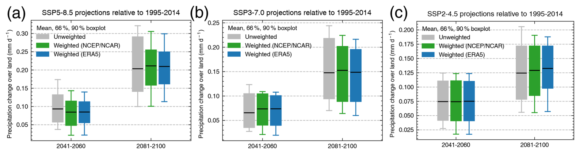
Figure 5 Boxplots of weighted and unweighted projections of precipitation over land relative to 1995–2014 for (a) the SSP5-8.5, (b) SSP3-7.0, and (c) SSP2-4.5 scenarios. The gray boxplots represent unweighted projections, the green boxplots represent projections weighted using NCEP–NCAR as a reference, and the blue boxplots represent projections weighted using ERA5 as a reference. Each boxplot displays the mean (solid black line), likely ranges (17th–83rd percentile), and very likely ranges (5th–95th percentile). The y axis indicates the precipitation change over land, while the x axis indicates the target period.

Given that the causal weighting accounts for models that better represent the dynamical pattern of SLP globally, we also examine the spatial pattern of precipitation change over land under global warming. Figure 6a–c show the spatial distribution of the causally weighted projections of mean precipitation changes for three SSP scenarios (SSP2-4.5, SSP3-7.0, and SSP5-8.5) for the period 2081–2100 relative to 1995–2014. ERA5 was used as a reference for the causal weighting. The projections indicate substantial regional variability across all scenarios. Significant increases in mean precipitation are projected in northern Europe, northern Asia, and parts of North America, as well as in East and South Asia and central and eastern Africa. These regions could see increases of up to 1.2 mm d⁻¹ under the SSP5-8.5 scenario. Conversely, decreases in precipitation are projected for the Mediterranean basin, Central America, and northern South America, with reductions reaching up to $-\mathrm{1.2}\mathrm{mm}{\mathrm{d}}^{-\mathrm{1}}$. These trends are consistent across all three SSP scenarios, though the intensity varies, with the most pronounced changes observed under the SSP5-8.5 scenario.

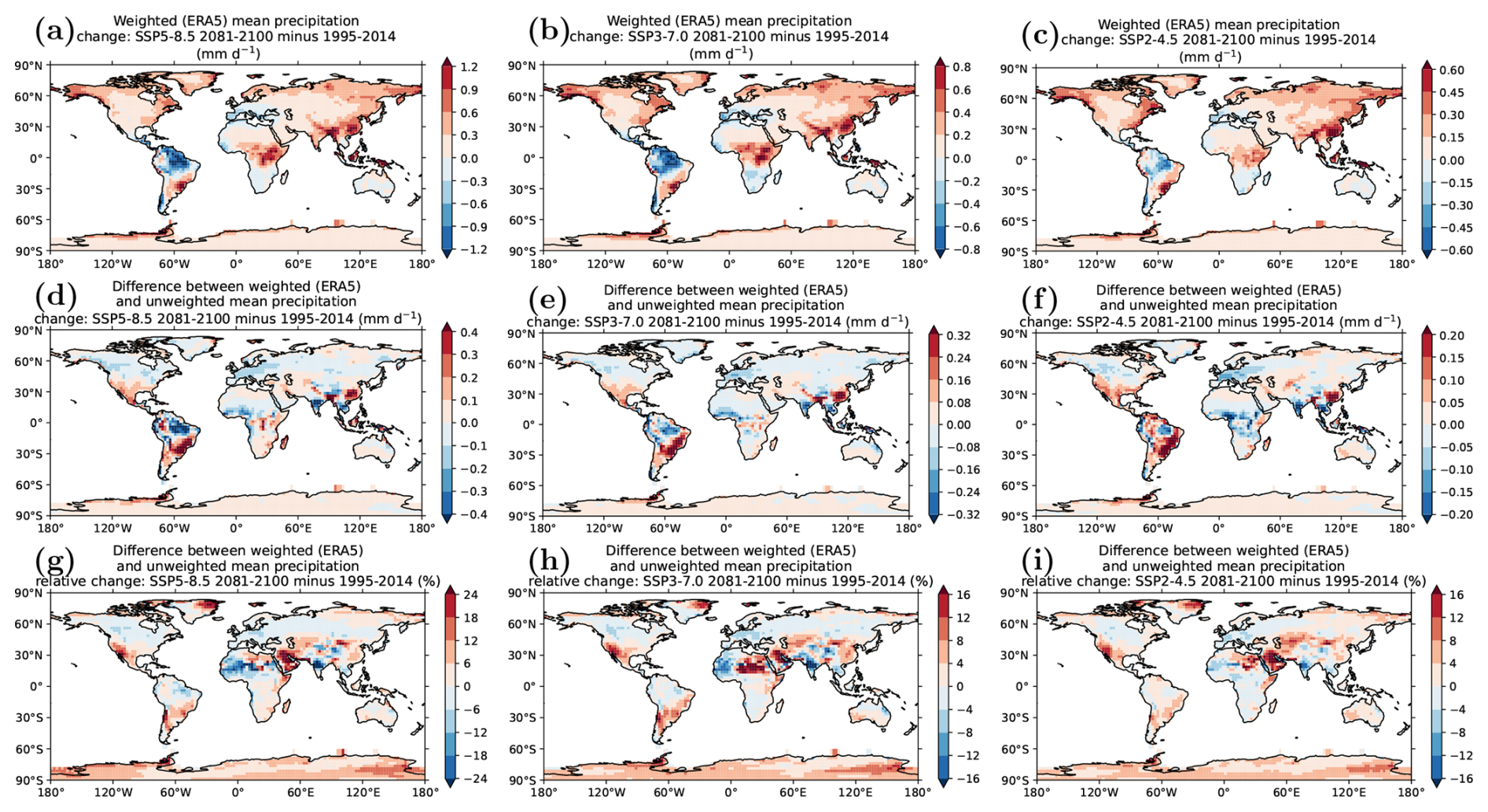
Figure 6 Patterns of causally weighted projections of mean precipitation change over land for the period 2081–2100 relative to 1995–2014 for the (a) SSP5-8.5, (b) SSP3-7.0, and (c) SSP2-4.5 scenarios. The differences between the weighted and unweighted mean precipitation change are shown in (d) for SSP5-8.5, (e) for SSP3-7.0, and (f) for SSP2-4.5. The differences between the weighted and unweighted mean precipitation relative change are shown in (g) for SSP5-8.5, (h) for SSP3-7.0, and (i) for SSP2-4.5. ERA5 was used as a reference for the causal weighting.

Figure 6d–f present the difference between the absolute changes in the causally weighted and unweighted mean for the period 2081–2100 relative to 1995–2014, while Fig. 6g–i depict the difference between the relative changes in the causally weighted and unweighted mean. Despite the spatially averaged weighted projections of precipitation change over land showing no significant deviation from the unweighted averages (refer to Fig. 5), Fig. 6d–i highlight that the weighted patterns exhibit notable spatial variations compared to the unweighted mean precipitation absolute change. Regions with positive absolute differences indicate areas where the weighted projections forecast greater increases in precipitation relative to the unweighted mean. Conversely, negative absolute differences denote areas where the weighted projections give smaller increases or larger decreases in precipitation than the unweighted mean. In particular, South America demonstrates the most significant variations in the weighted projections, with absolute differences reaching up to $\pm \mathrm{0.4}\mathrm{mm}{\mathrm{d}}^{-\mathrm{1}}$. However, the map of differences between the relative changes in the weighted and unweighted mean precipitation suggests that these absolute changes are not the largest relative changes globally. The regions of the Sahara, the Arabian Peninsula, southwestern South America and North America, and northeastern Greenland exhibit more pronounced relative changes, with values reaching up to 20 %.

A figure comparable to Fig. 6 is presented in Fig. F1 of the Appendix, illustrating the projected changes for the period 2041–2060. The observed trends for 2081–2100 remain consistent for this earlier period.

4 Summary and discussion

Climate projections derived from an ensemble of multiple climate models participating in the Coupled Model Intercomparison Project Phase 6 (CMIP6; Eyring et al., 2016) continue to have large uncertainties for precipitation (Tebaldi et al., 2021). This hinders the delivery of accurate information for mitigation and adaptation. Eyring et al. (2019) argue that advanced methods for model weighting are needed to distill more credible information on regional climate changes, pointing out the importance of considering both model performances and interdependencies in model weighting studies as for example presented by Knutti et al. (2017) and Brunner et al. (2020). Machine learning can play an important role in pushing the frontiers of climate model analysis (Eyring et al., 2024a), including approaches to weight multimodel projections (Schlund et al., 2020a). Here we build on a previous study that evaluates the performance of a CMIP ensemble with causal networks (Nowack et al., 2020) and expand this concept to a weighting scheme for precipitation projections with causal discovery.

We first demonstrate that causal model evaluation of CMIP6 models can effectively identify specific causal fingerprints of sea level pressure (SLP) that influence precipitation patterns and their projections. Notably, we identify a parabolic relationship between the ability of climate models to represent observed dynamical SLP patterns in causal networks, quantified by the networks' F₁ scores, and the projected precipitation changes over land by the end of the century. CMIP6 models that better represent reference dynamical interactions in their causal networks produce projections within the middle range of the CMIP6 ensemble, while models with lower skill either overestimate or underestimate the mean projections. This pattern is consistent across various global warming scenarios (SSP2-4.5, SSP3-7.0, and SSP5-8.5) and reference reanalysis datasets (NCEP–NCAR and ERA5). Similar findings were reported by Nowack et al. (2020) for the RCP8.5 simulations of CMIP5 models.

Additionally, our study reveals that CMIP6 models with shared development, such as those with a common ancestor model or the same atmospheric model, exhibit more similar causal pathways. This result underscores the ability of the causal model evaluation to effectively identify interdependencies of the CMIP6 models.

Building on these findings, the study introduces a causal weighting scheme for climate projections based on the performance and interdependence of their causal networks. By combining causal model evaluation with multimodel weighting, this approach offers a convincing alternative to traditional weighting based on metrics such as root-mean-square error or trend analysis (Knutti et al., 2017; Brunner et al., 2020; Liang et al., 2020; Tokarska et al., 2020).

The implementation of this causal weighting scheme for projecting precipitation over land significantly reduces the uncertainty range of the climate projections. While the weighted mean projections are closely aligned with the unweighted means, the likely (17th–83rd percentile) and very likely (5th–95th percentile) weighted ranges were notably narrower, and the spatial patterns revealed regional differences in precipitation. For the end-of-century period, 2081–2100, the sizes of the very likely weighted ranges under SSP2-4.5, SSP3-7.0, and SSP5-8.5 are reduced by 10 % to 16 %, while the likely ranges show an even greater reduction, ranging from 16 % to 41 %, when ERA5 was used as a reference.

For future research, we consider several areas to be particularly promising. One potential direction is the development of multi-diagnostic weighting (Schlund et al., 2020a), which involves integrating multiple metrics alongside the SLP causal network distance metric into the weighting process. This multi-diagnostic approach could improve precipitation projections further by addressing model differences more comprehensively. By considering additional diagnostics, such as temperature trends, weighted projections may further reduce the uncertainty in projected precipitation over land. Another promising direction is the regional weighting of precipitation change. This approach would focus the weighting scheme specifically on regional precipitation projections, incorporating both global and region-specific diagnostics. Tailoring multimodel weighting to specific regions could prove especially effective. Exploring alternative similarity measures is also a key area for future investigation. Currently, F₁ scores are used to measure the similarity between causal networks, but alternative measures that better discriminate between causal networks or that consider causal effects could provide new insights.

Finally, we want to emphasize that our methodology is not limited to projecting precipitation changes over land. Its applicability could extend to any target variable, provided that pertinent variables and diagnostics exhibiting a robust and consistent relationship (e.g., a parabolic relationship) with the target variable are selected. Our results highlight the importance of integrating advanced evaluation methods and weighting schemes to reduce the uncertainty ranges of climate projections (Nowack and Watson-Parris, 2025). Alongside the development of improved hybrid Earth system models with machine learning with demonstrated reduction in long-standing systematic errors (Eyring et al., 2024a, b), this research provides a novel methodology to constrain uncertainties in multimodel climate projections towards more robust climate change information and more effective mitigation and adaptation strategies.

Appendix A: Maps of sea level pressure components

In Figs. A1 and A2, we show the centers of the first 60 PCA–varimax components. By comparing the spatial patterns for each season between ERA5 and NCEP–NCAR, we can observe similarities and differences in the distribution of components. Generally, we see similar large-scale patterns since both datasets are reanalyses of atmospheric variables. However, differences arise due to variations in data assimilation methods and model physics. PCA–varimax identifies major modes of variability for all seasons and datasets, as reported in Vejmelka et al. (2015) and Nowack et al. (2020). The components explaining the most variance are located in the tropics (for example the El Niño region), influencing atmospheric circulation globally.

A1 NCEP–NCAR components

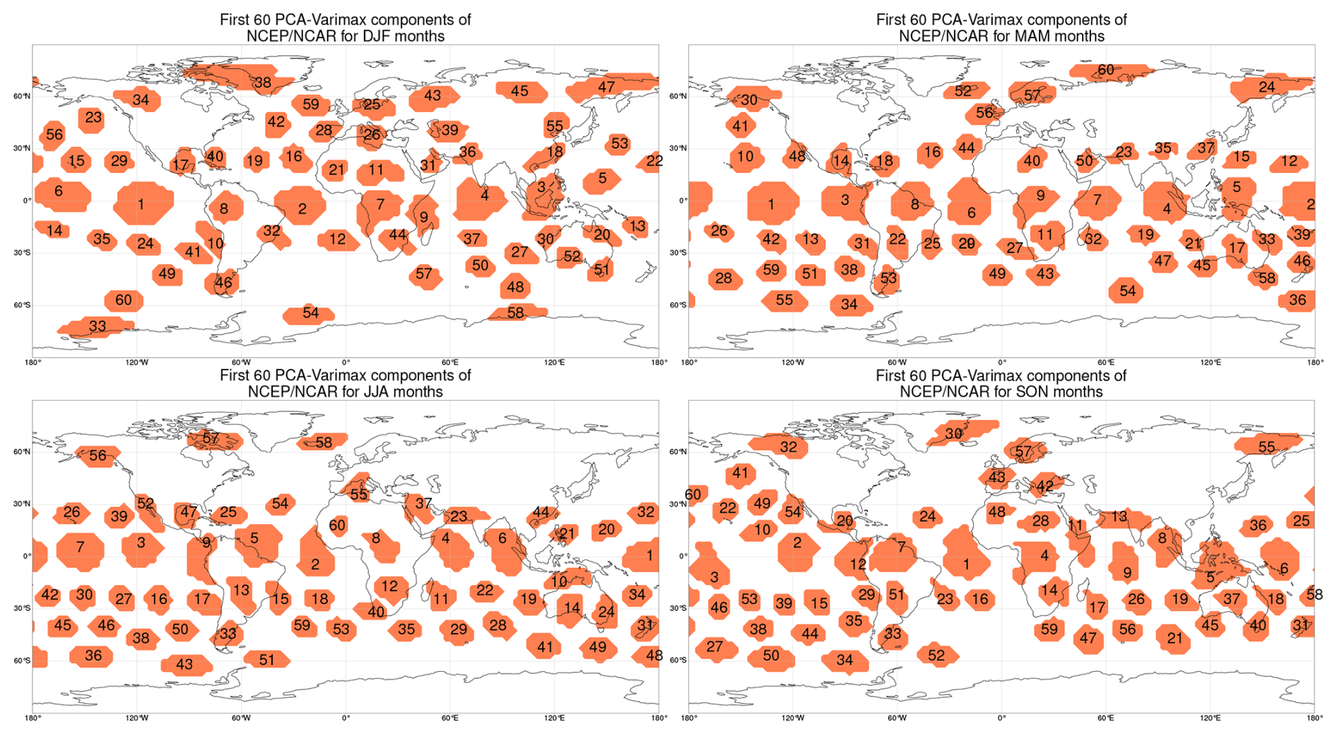
Figure A1 Principal component analysis (PCA) with varimax rotation for the NCEP–NCAR dataset during DJF (December, January, February), MAM (March, April, May), JJA (June, July, August), and SON (September, October, December). Here, each component is represented by its core, which consists of loadings greater than 80 % of the maximum loading.

A2 ERA5 components

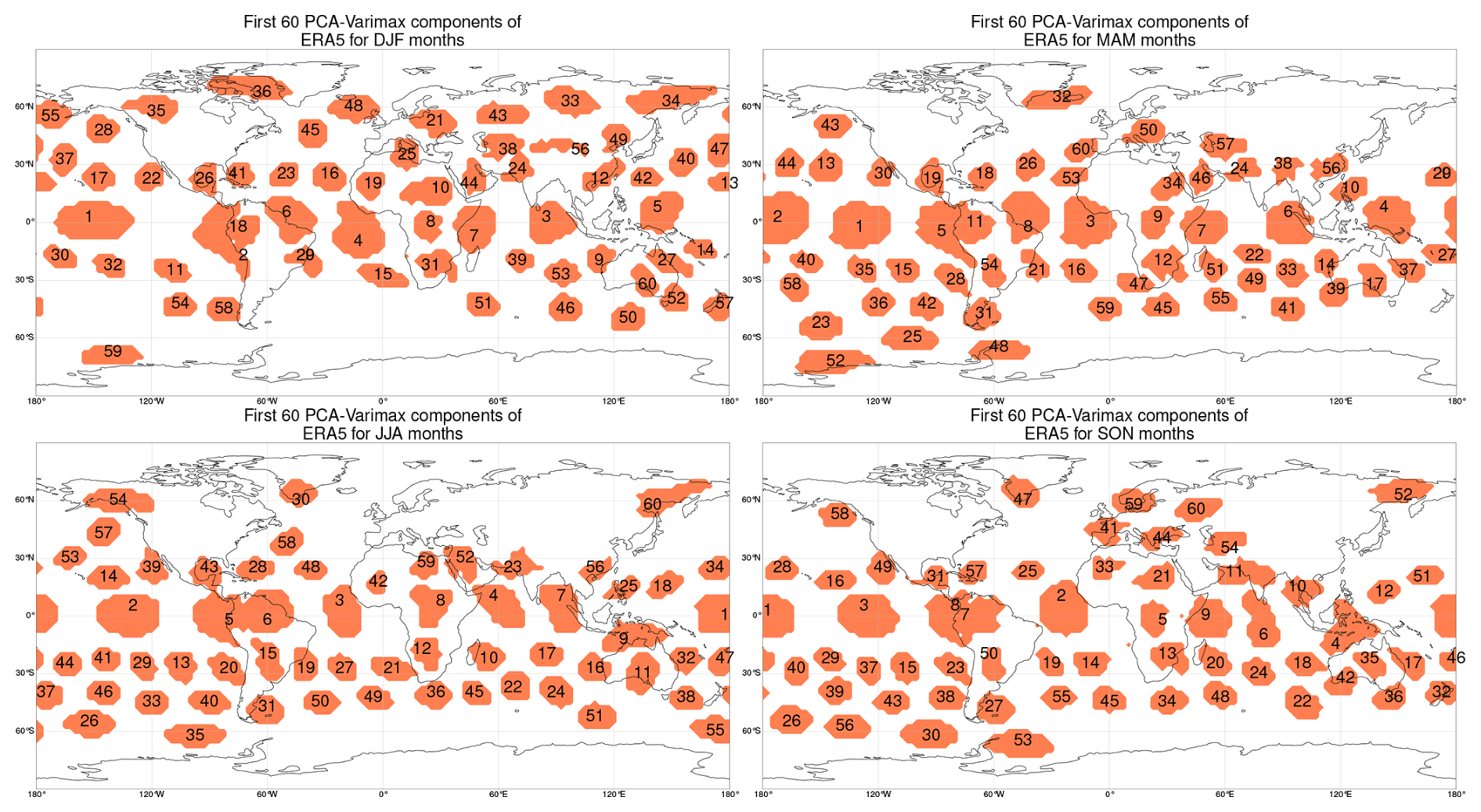
Figure A2 Principal component analysis (PCA) with varimax rotation for the ERA5 dataset during DJF (December, January, February), MAM (March, April, May), JJA (June, July, August), and SON (September, October, December). Here, each component is represented by its core, which consists of loadings greater than 80 % of the maximum loading.

Appendix B: Causal network estimation results

Although a maximum time lag of 20 d was set for PCMCI, 99.9 % of the dependencies were found within the first 10 d. The causal networks are too complex to visualize, with an average of 18 causal dependencies per mode for NCEP–NCAR and 20 for ERA5. For this reason, we choose to inspect only the most significant causal dependencies of each mode. Figure B1 displays the most significant causal dependencies for each mode in the two reanalysis datasets during the winter months (DJF). Despite the lack of spatial information provided to the PCMCI causal discovery algorithm, the most significant dependencies predominantly originate from neighboring modes, indicating that the causal network estimation step identifies physically meaningful dependencies between the SLP modes for both reanalysis datasets.

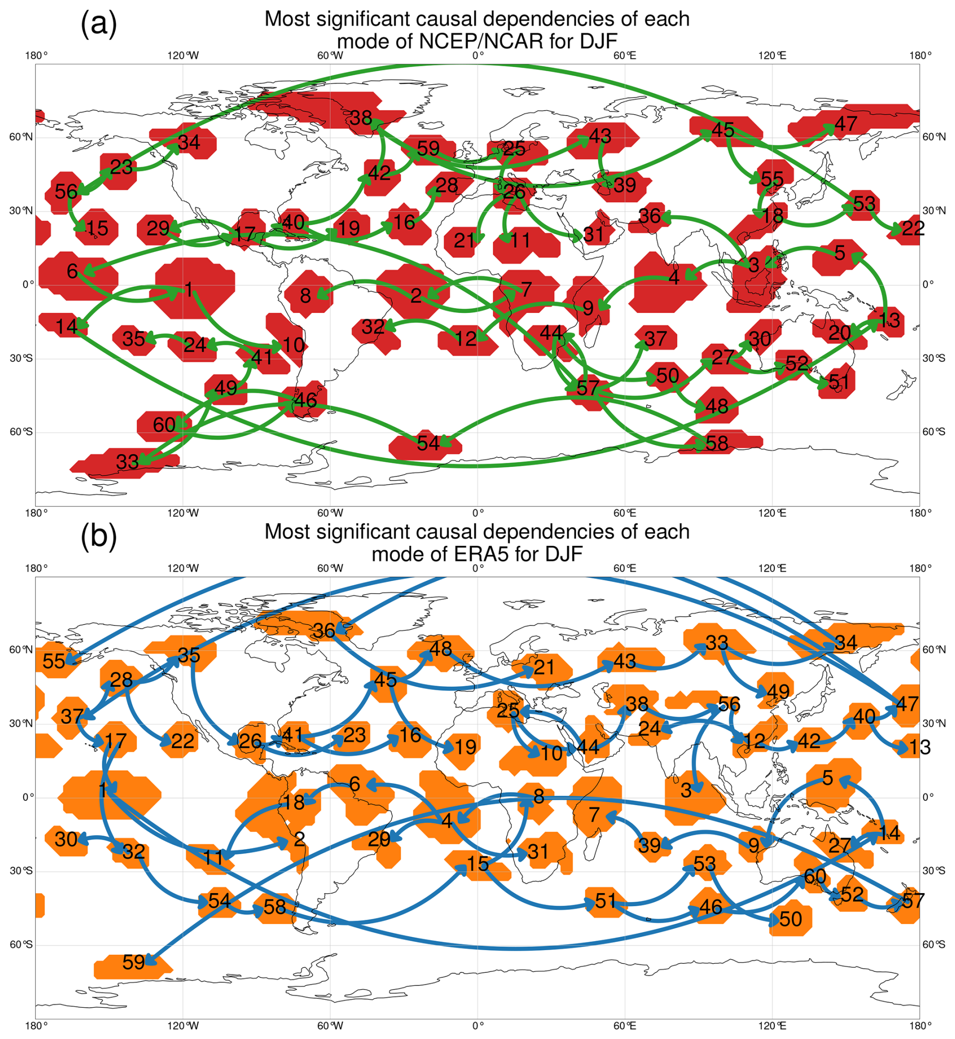
Figure B1 Most significant causal dependencies of each mode in DJF (December, January, February) for the (a) NCEP–NCAR or (b) ERA5 dataset. The PCMCI causal discovery algorithm identifies physically meaningful links. Despite the lack of spatial information provided to the algorithm, the most significant dependency for a mode generally originates from a neighboring mode. Each mode has, on average, 18 or 20 causal dependencies for NCEP–NCAR or ERA5, respectively, with time lags ranging from 1 to 20 d. Notably, 99.9 % of these dependencies are found with a time lag of less than 10 d.

Appendix C: Causal network evaluation results

For Fig. 2, the Spearman rank correlation coefficient is calculated between the rankings of climate models to assess variation in rankings across the different reference datasets (NCEP–NCAR and ERA5), yielding a coefficient of 0.91. This confirms a strong consistency between the climate model rankings with the NCEP–NCAR and ERA5 references. The obtained p value from the Student t test is $\mathrm{1.1}\times {\mathrm{10}}^{-\mathrm{9}}$, rejecting the null hypothesis of no ordinal correlation between the rankings of models with NCEP–NCAR or ERA5 taken as reference. In Fig. C1, we compare the climate models' causal networks' F₁ scores relative to the NCEP–NCAR and ERA5 reference datasets across different seasons (DJF, MAM, JJA, and SON). Although the structure of the causal networks exhibits substantial seasonal variation, the comparison of F₁ scores consistently highlights similar performance patterns across seasons. This consistency reinforces the validity of using season-averaged F₁ scores in the rest of this study.

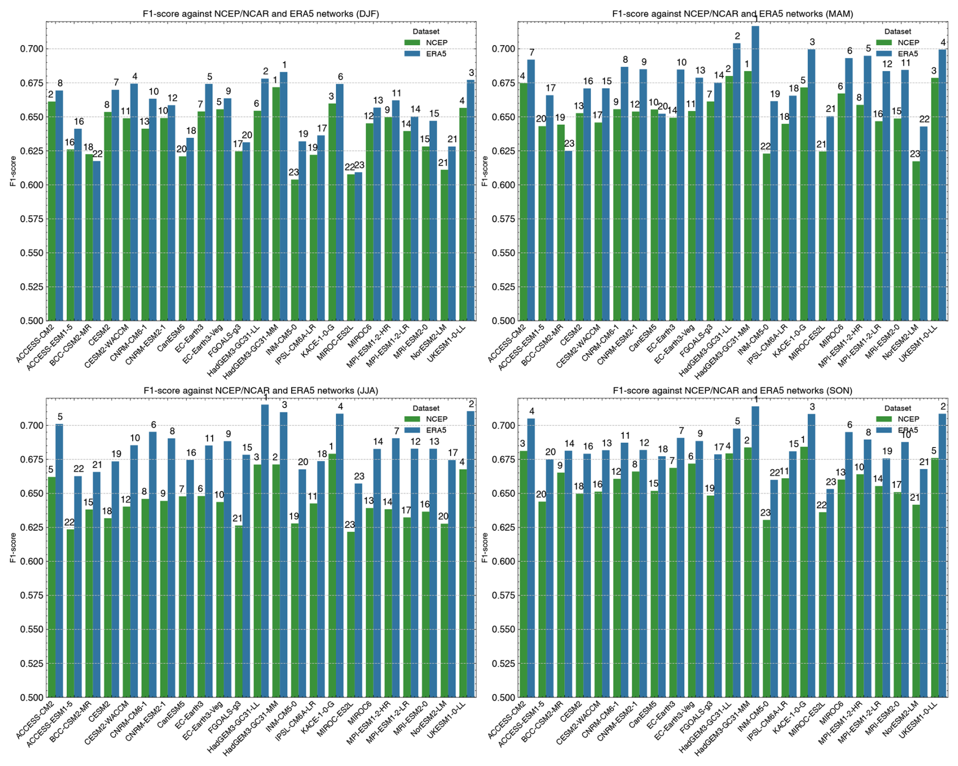
Figure C1 Comparison of the climate models' causal networks' F₁ scores with NCEP–NCAR (green) and ERA5 (blue) as reference for the four meteorological seasons. This figure illustrates the similarity between climate models' causal networks and those of the reference reanalysis datasets, averaged across all available members, using the F₁ score. Higher F₁ scores indicate greater similarity. The rank of each model's similarity is denoted on top of each bar.

Appendix D: Impact of the number of modes, maximum time lag of PCMCI, and α_MCI

In Fig. D1, we vary the significance level α_MCI of PCMCI from 10⁻⁵ to 10⁻⁴ and 10⁻³. Figure D2 demonstrates the effects of reducing the number of modes in the networks from 60 to 50 and decreasing the maximum time lag in the PCMCI algorithm from 20 to 10 d. While these variations affected the F₁ score values moderately, they had a minimal influence on the rankings of the climate models. This was evaluated by calculating the Spearman rank correlation coefficient for the modified experiments against the baseline experiment presented in the main text (Fig. 2a), which used the NCEP–NCAR reference with 60 modes and ${\mathit{\alpha }}_{\text{MCI}}={\mathrm{10}}^{-\mathrm{5}}$. The correlation coefficients were close to 1, ranging from 0.95 to 0.98, confirming a strong ordinal correlation between the rankings of models in the different experiments. The p values, all smaller than 10⁻¹¹, rejected the null hypothesis of no ordinal correlation between the alternative experiments and the baseline experiment.

D1 Impact of α_MCI on the causal model evaluation step

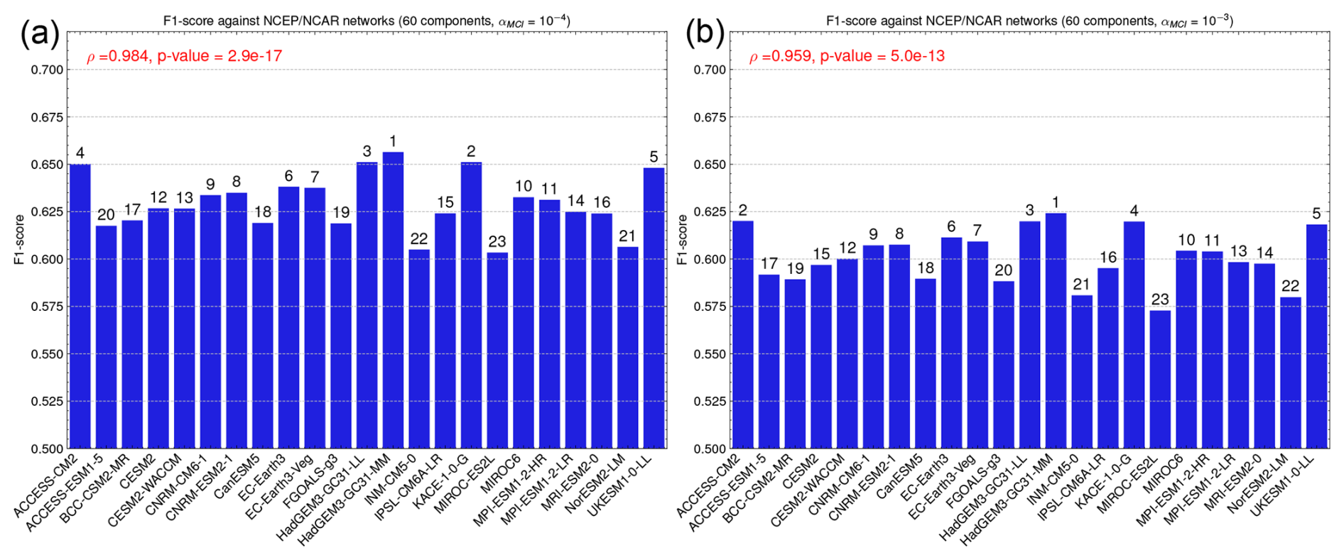
Figure D1 Impact of α_MCI on climate models' causal networks' F₁ scores with NCEP–NCAR as reference. The causal networks, composed of 60 modes, were constructed using varying levels of α_MCI. Specifically, α_MCI is varied from (a) 10⁻⁴ to (b) 10⁻³, whereas ${\mathit{\alpha }}_{\text{MCI}}={\mathrm{10}}^{-\mathrm{5}}$ is used in the main text. α_MCI represents the significance level for the MCI step in PCMCI. A causal link is established if the MCI test value is equal to or smaller than α_MCI. The Spearman rank correlation coefficient was calculated to compare the variation in model rankings relative to the main text results in Fig. 2a. The resulting Spearman rank correlation coefficient and the associated p value from a Student t test, testing the null hypothesis of no ordinal correlation between the rankings, are displayed in red.

D2 Impact of the number of modes and maximum time lag on the causal model evaluation step

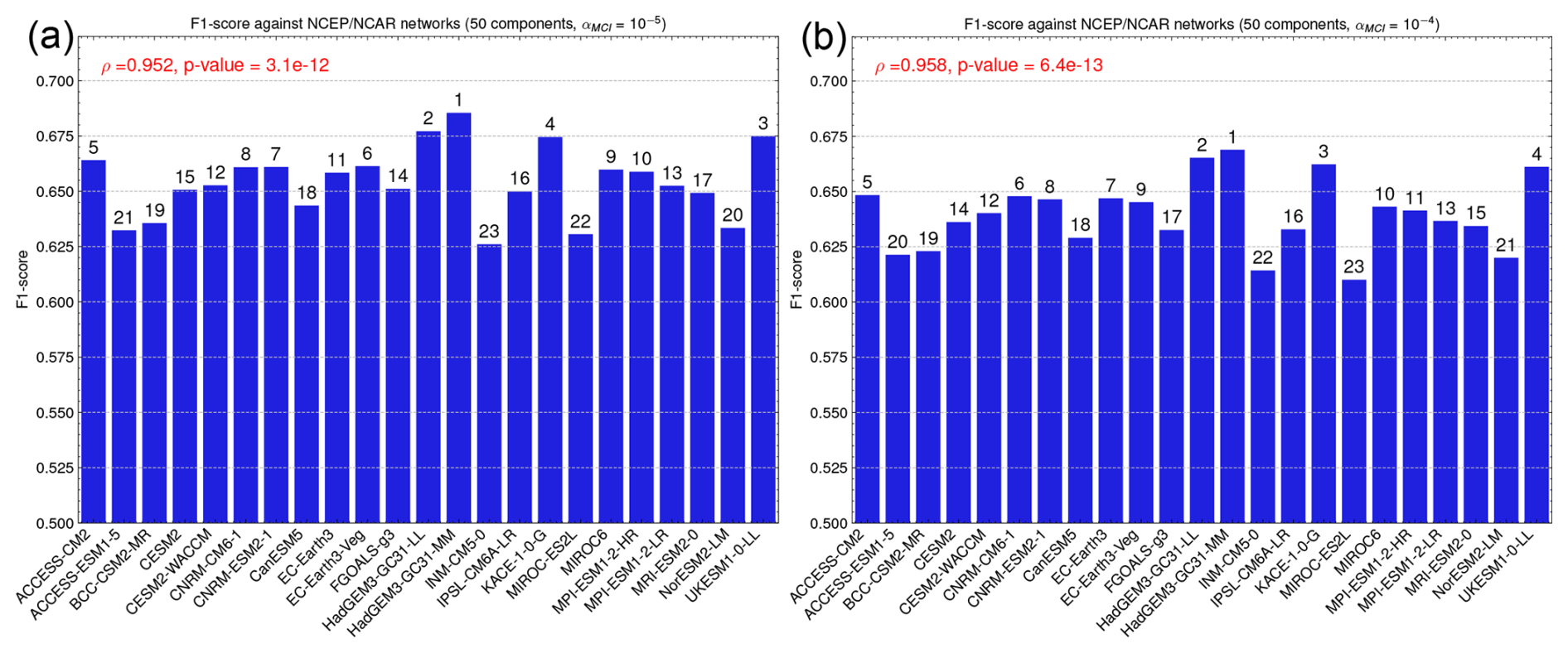
Figure D2 Impact of the number of PCA–varimax modes on climate models' causal networks' F₁ scores with NCEP–NCAR as reference. The causal networks are composed of 50 modes, in contrast to the 60 modes used in the main text. Additionally, the maximum time lag in PCMCI is set to 10 d instead of 20 d. The parameter α_MCI of PCMCI is also varied from (a) 10⁻⁵ to (b) 10⁻⁴. The Spearman rank correlation coefficient was calculated to compare the variation in model rankings relative to the main text results in Fig. 2a. The resulting Spearman rank correlation coefficient and the associated p value from a Student t test, which tests the null hypothesis of no ordinal correlation between the rankings, are displayed in red at the top of each subfigure.

Appendix E: Calibration of interdependence shape parameter σ_S

In Fig. E1, we note that internal variability itself offers opportunities to learn about the robustness of our method. Specifically, we have found differences between the causal networks of the models, which were shown to be larger than the differences between the causal networks across ensemble members of individual models. This supports the idea that the differences we capture are meaningful and not purely due to internal variability. This finding aligns with results from previous work (Nowack et al., 2020), where this was demonstrated clearly.

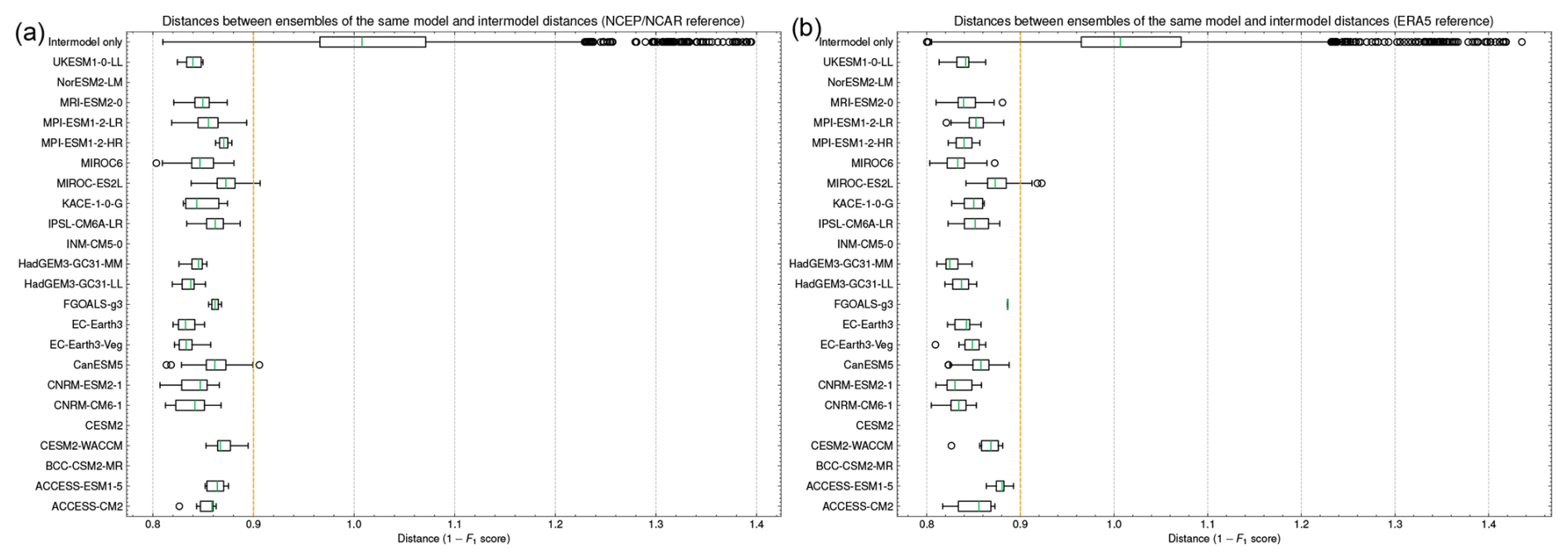
Figure E1 Distances between ensembles of the same model and intermodel distances for (a) NCEP–NCAR and (b) ERA5 taken as reference. The distances are calculated using the complement of the F₁ scores normalized by the median across all models. σ_S is set to 0.9 (dashed orange line), which separates most of the intermodel distances and the intramodel distances.

Appendix F: Weighted projections of land precipitation changes

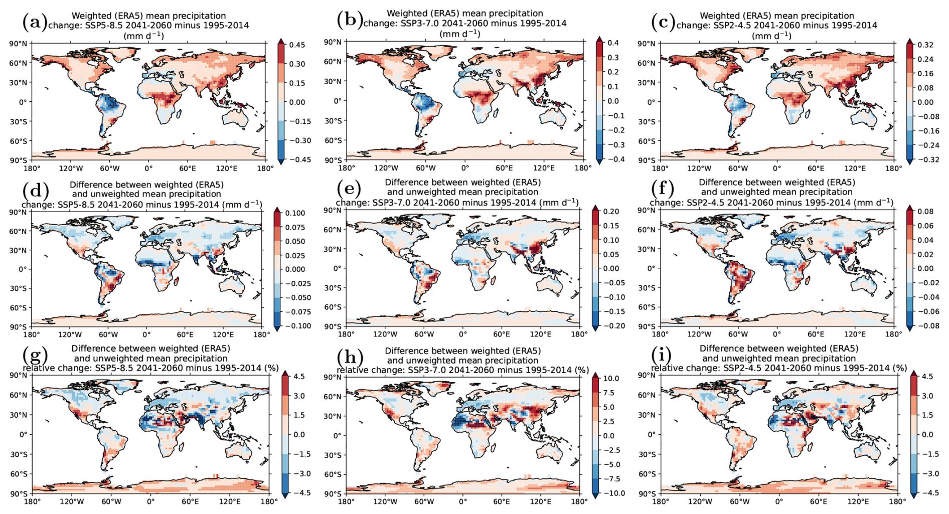
Figure F1 Patterns of causally weighted projections of mean precipitation change over land in the period 2041–2060 relative to 1995–2014 for the (a) SSP5-8.5, (b) SSP3-7.0, and (c) SSP2-4.5 scenarios. The differences between the weighted and unweighted mean precipitation change are shown in (d) for SSP5-8.5, (e) for SSP3-7.0, and (f) for SSP2-4.5. The differences between the weighted and unweighted mean precipitation relative change are shown in (g) for SSP5-8.5, (h) for SSP3-7.0, and (i) for SSP2-4.5. ERA5 was used as a reference for the causal weighting.