the Creative Commons Attribution 4.0 License.
the Creative Commons Attribution 4.0 License.
 | 13 Mar 2024
Hemispherically symmetric strategies for stratospheric aerosol injection
Yan Zhang
Douglas G. MacMartin
Daniele Visioni
Ewa M. Bednarz
Ben Kravitz
Stratospheric aerosol injection (SAI) comes with a wide range of possible design choices, such as the location and timing of the injection. Different stratospheric aerosol injection strategies can yield different climate responses; therefore, understanding the range of possible climate outcomes is crucial to making informed future decisions on SAI, along with the consideration of other factors. Yet, to date, there has been no systematic exploration of a broad range of SAI strategies. This limits the ability to determine which effects are robust across different strategies and which depend on specific injection choices. This study systematically explores how the choice of SAI strategy affects climate responses in one climate model. Here, we introduce four hemispherically symmetric injection strategies, all of which are designed to maintain the same global mean surface temperature: an annual injection at the Equator (EQ), an annual injection of equal amounts of SO2 at 15° N and 15° S (15N+15S), an annual injection of equal amounts of SO2 at 30° N and 30° S (30N+30S), and a polar injection strategy that injects equal amounts of SO2 at 60° N and 60° S only during spring in each hemisphere (60N+60S). We compare these four hemispherically symmetric SAI strategies with a more complex injection strategy that injects different quantities of SO2 at 30° N, 15° N, 15° S, and 30° S in order to maintain not only the global mean surface temperature but also its large-scale horizontal gradients. All five strategies are simulated using version 2 of the Community Earth System Model with the middle atmosphere version of the Whole Atmosphere Community Climate model, version 6, as the atmospheric component, CESM2(WACCM6-MA), with the global warming scenario, Shared Socioeconomic Pathway (SSP)2-4.5. We find that the choice of SAI strategy affects the spatial distribution of aerosol optical depths, injection efficiency, and various surface climate responses. In addition, injecting in the subtropics produces more global cooling per unit injection, with the EQ and the 60N+60S cases requiring, respectively, 59 % and 50 % more injection than the 30N+30S case to meet the same global mean temperature target. Injecting at higher latitudes results in larger Equator-to-pole temperature gradients. While all five strategies restore Arctic September sea ice, the high-latitude injection strategy is more effective due to the SAI-induced cooling occurring preferentially at higher latitudes. These results suggest trade-offs wherein different strategies appear better or worse, depending on which metrics are deemed important.
- Article
(2961 KB) - Full-text XML
- Companion paper
-
Supplement
(1755 KB) - BibTeX
- EndNote


Current climate projections suggest that under most emission scenarios, the 1.5 °C threshold of global mean temperature increase above pre-industrial levels set by the Paris Agreement is likely to be exceeded by 2040 or earlier (IPCC, 2021; Tebaldi et al., 2021; Dvorak et al., 2022). Meinshausen et al. (2022) showed that implementing all conditional and unconditional Paris Agreement pledges on time may limit global warming to just below 2 °C. With the uncertainties in the implementation of carbon emission reductions, estimates of climate sensitivity, and severity of the impacts of climate change, only relying on carbon emission reduction is likely insufficient to reduce the possibility of severe adverse climate impacts in the foreseeable future (Rogelj et al., 2016; Bamber et al., 2019; Anderson et al., 2020; Sherwood et al., 2020; Bjordal et al., 2020; MacMartin et al., 2022). This leads to the suggestion that stratospheric aerosol injection (SAI) could be an option at some point to reduce severe adverse impacts on climate and society. Such an approach would consist of injecting aerosols, or their precursors, in the lower stratosphere to reflect a small fraction of the incoming solar radiation back to space, lowering the global mean temperature as a result. In this study, we focus only on SO2 injections.
To inform future decisions on SAI deployment, it is important to have a sufficient understanding of the range of possible climate responses under SAI; these would depend on both the scenario and strategy. However, most existing SAI studies looking at surface impacts consider only a single scenario (i.e., a particular choice of background emission scenario, deployment start date, and desired temperature target to be achieved with SAI) and only look at a single SAI strategy (i.e., a particular choice of injection latitude(s) and season(s)) (Kravitz et al., 2019; Visioni et al., 2020b; Tilmes et al., 2018; Irvine et al., 2019). Recently, MacMartin et al. (2022) and Visioni et al. (2023b) explored a set of specific scenario choices that cover a range of plausible futures, all with a single strategy. Here we consider and compare a set of different SAI strategies under the same scenario. Collectively, MacMartin et al. (2022) and this study capture two key dimensions of the range of possible climate responses to SAI.
Different SAI strategies could result in the same level of global cooling but affect the regional surface climate differently (Visioni et al., 2020b; Kravitz et al., 2019; Lee et al., 2020, 2021; Zhang et al., 2022). Injecting SO2 at the Equator would overcool the tropical region and undercool the high-latitude regions (Kravitz et al., 2019); this was a key motivation for developing a multi-objective strategy in Kravitz et al. (2017) that injects at multiple latitudes to balance not just global mean temperature but also interhemispheric and Equator-to-pole temperature gradients. This multi-objective strategy was used in the Geoengineering Large Ensemble Project (GLENS; Tilmes et al., 2018) and more recent studies (MacMartin et al., 2022; Richter et al., 2022). Injecting at 60° N would primarily cool the Northern Hemisphere (Lee et al., 2023a). Injecting SO2 in the same latitude but in different seasons may also result in slightly different regional climate responses (Visioni et al., 2020b). Knowing the dependence of various climate responses on the choice of SAI strategies is crucial for comparing the benefits and risks of different SAI strategies. In addition, SAI will not bring the climate back to the same state as lowering the CO2 concentration; instead, it will create a novel climate (Bala et al., 2010; Niemeier and Timmreck, 2015; Kravitz et al., 2017; Tilmes et al., 2018; Irvine et al., 2019). Knowing the range of possible climates and how close we can bring the climate to a reference state by SAI will enable us to evaluate the limits of SAI and the trade-offs between achieving different climate goals.
In this study, we simulate four hemispherically symmetric injection strategies in order to explore the range of possible climate responses. These four strategies are the annual injection of SO2 at the Equator (EQ), annual injection of equal amounts of SO2 at 15° N and 15° S (15N+15S), annual injection of equal amounts of SO2 at 30° N and 30° S (30N+30S), and spring injection of equal amounts of SO2 at 60° N and 60° S (60N+60S; it is referred to as POLAR in Bednarz et al., 2023a, and Polar+1.0 in Goddard et al., 2023), all designed to maintain a targeted global mean temperature. We assess a broad range of differences between these strategies to illustrate trade-offs between them; this understanding can lay the foundation for future work to develop better strategies and motivate the design of future multi-model intercomparisons. Section 2 describes the climate model used herein. Section 3 explains how this set of strategies is chosen and describes the simulation setup. Section 4 describes the simulation results of the four new strategies and compares them to the multi-objective strategy developed in Kravitz et al. (2017) and simulated in MacMartin et al. (2022) (see also the companion paper Bednarz et al., 2023a, that compares the stratospheric response for these strategies).
All SAI strategies are simulated using version 2 of the Community Earth System Model with the middle atmosphere version of the Whole Atmosphere Community Climate model, version 6, as the atmospheric component, CESM2(WACCM6-MA) (Danabasoglu et al., 2020; Gettelman et al., 2019; Davis et al., 2023). CESM2(WACCM6-MA) is a fully coupled Earth system model which includes atmosphere, ocean, land, and sea ice components. The middle atmosphere (MA) version of WACCM6 uses chemistry mechanisms relevant for the stratosphere and mesosphere with a reduced set of tropospheric reactions (Davis et al., 2023), similar to the chemistry configuration in CESM1(WACCM). The ocean component is based on the Parallel Ocean Program Version 2 (POP2), the land component is Community Land Model Version 5 (CLM5), and the sea ice component is CICE5 (Danabasoglu et al., 2020). The horizontal resolution of CESM2(WACCM6-MA) is 0.95° in latitude and 1.25° in longitude, with 70 vertical layers extending from the Earth's surface to about 140 km in altitude, the same as in CESM1(WACCM) (Mills et al., 2017). The stratospheric aerosol distribution in this model reasonably matches observations after the 1991 eruption of Mount Pinatubo (Mills et al., 2017).
While different SAI strategies would not result in the same surface climate, the differences in surface climate responses between some SAI strategies would be much easier to detect than between others. The detectability of the differences in surface climate responses between SAI strategies depends on, among other factors, the level of global cooling and natural variability. Zhang et al. (2022) estimated based on Community Earth System Model (CESM1) simulations that for a SAI-induced global cooling of 1–1.5 °C, there are only six to eight injection choices that would produce detectably different surface climate responses, where two injection choices are considered detectably different if the difference in temperature or precipitation responses are detectable at a 95 % confidence level over a 20-year period on more than 5 % of the Earth's area. Although the estimate of six to eight distinct injection choices was made using CESM1(WACCM) simulations, the conclusion is expected to hold relatively well in CESM2(WACCM), due to similarities in the stratospheric circulation and aerosol microphysics between the two model versions. This is demonstrated by the results of a set of fixed-amount single-latitude injection simulations (Fig. S1 in the Supplement). For a global cooling level of 1–1.5 °C, a reasonable choice of seven latitudes of injection with patterns of aerosol optical depth (AOD) that would yield detectably different surface climate responses is 60° N, 30° N, 15° N, the Equator, 15° S, 30° S, and 60° S (Zhang et al., 2022). These seven latitudes could be combined in different ways to form a set of seven linearly independent injection strategies that span the same AOD design space. The outcomes of other strategies can be estimated by a linear combination of these seven injection strategies, assuming linearity (MacMartin et al., 2017, 2019; Zhang et al., 2022).
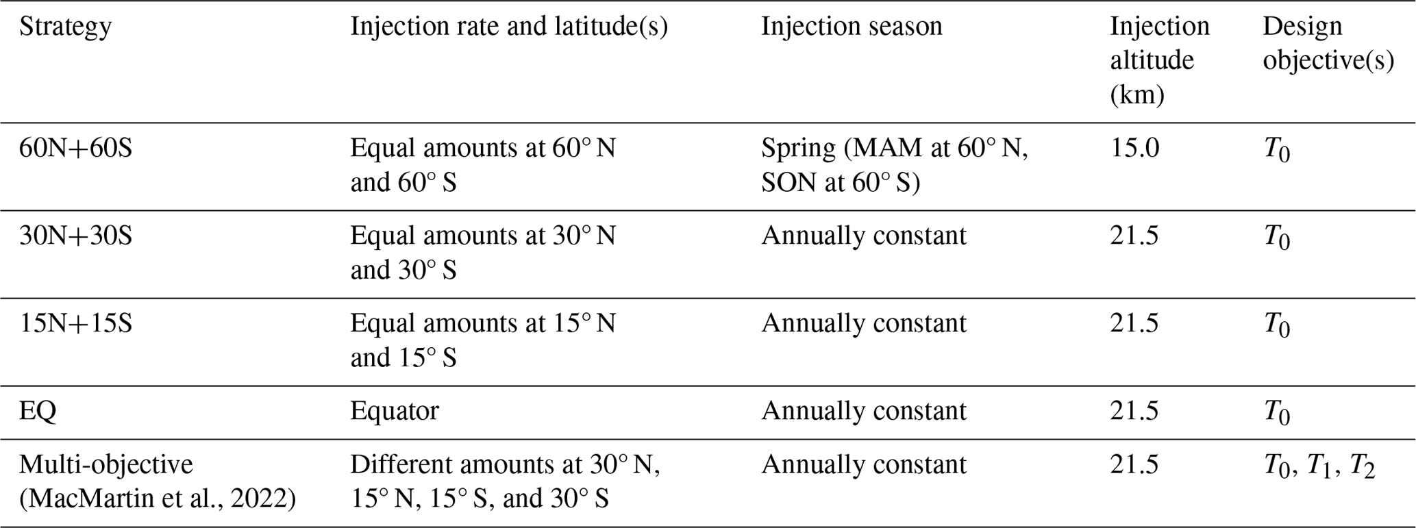
Here, we simulate and compare four hemispherically symmetric injection strategies that collectively cover the seven latitudes mentioned above, with the consideration of ensuring hemispheric equality in the deployment of SAI. These four injection strategies are injecting solely at the Equator (EQ), injecting the same amount at 15° N and 15° S (15N+15S), injecting the same amount at 30° N and 30° S (30N+30S), and injecting the same amount at 60° N and 60° S in springtime only in each hemisphere (60N+60S) (Table 1). These new strategies are designed to maintain the same global mean surface temperature (T0). The global mean surface temperature is the metric used by the United Nations Framework Convention on Climate Change (UNFCCC) to operationalize climate change goals in the Paris Agreement (UNFCCC, 2015) and is thus a reasonable metric to consider a target for SAI (MacMartin et al., 2022). In addition, we compare the new strategies simulated herein with a multi-objective strategy simulated in MacMartin et al. (2022) that maintains not only T0 but also the interhemispheric temperature gradient (T1) and Equator-to-pole temperature gradient (T2).
The multi-objective strategy adjusts the SO2 injection rates at 30° N, 15° N, 15° S, and 30° S to maintain T0, T1, and T2. Managing the interhemispheric temperature gradient is motivated by the desire to reduce shifts in tropical precipitation; however, the specific injection rates have been shown to vary even in different versions of the same Earth system model (Fasullo and Richter, 2023). While the radiative forcing from CO2 is roughly hemispherically symmetric, other effects such as rapid cloud responses to elevated CO2 levels and changes in the Atlantic meridional overturning circulation (AMOC) lead to changes in T1 that require asymmetric injection to compensate. These effects are model dependent; for example, in CESM1(WACCM), more injection is needed in the Northern Hemisphere (NH) to compensate T1, but in CESM2(WACCM6), more injection is needed in the Southern Hemisphere (SH) (Fasullo and Richter, 2023). Because the sign of the hemispheric asymmetry in injection rates that is needed to maintain T1 varies among different climate models, here we focus on hemispherically symmetric strategies that maintain only T0 (Table 1). While we do not expect these to fully balance the interhemispheric temperature gradient T1 in CESM2(WACCM6), these strategies are simpler to implement in other climate models, as the injection rate could be adjusted to meet the only objective (T0) by hand. Simultaneously tuning multiple variables is more challenging without explicitly coding a feedback control algorithm.
In addition to the multi-objective strategy and the four hemispherically symmetric strategies, a complete set of strategies spanning the space of the seven injection choices described by Zhang et al. (2022) would also include two other strategies, such as a spring injection at 60° N (Lee et al., 2023a) and an annually constant injection at 30° N (Bednarz et al., 2022). However, injecting outside of the tropics but in a single hemisphere would primarily cool that hemisphere, which would result in a significant perturbation of the interhemispheric temperature gradient and the associated location of tropical precipitation (Haywood et al., 2013). Thus, these or any other extratropical single-latitude injections are already known to not be an appropriate strategy for targeting global mean temperature and as such are not included in the analysis discussed here.
All of the strategies considered herein are simulated under the same scenario (i.e., the same background greenhouse gas emissions, start date for SAI deployment, and global mean temperature target). The background emission scenario used here is the Shared Socioeconomic Pathway (SSP) 2-4.5 (Meinshausen et al., 2020), a middle-of-the-road pathway in which the world is facing medium challenges to mitigation and adaptation (IPCC, 2021). This background emission scenario is roughly consistent with the Paris Agreement's Nationally Determined Contributions (Burgess et al., 2021; UNEP, 2021). All of these injection strategies are simulated from the beginning of 2035 to the end of 2069. The average over 2020–2039 in the model is chosen to be representative of when future climate might reach 1.5 °C above pre-industrial levels (MacMartin et al., 2022). Here, to increase the ability to distinguish between effects of different strategies, we choose an additional 0.5 °C cooling relative to the 1.5 °C target from the Paris Agreement. This new temperature target of 1.0 °C above pre-industrial levels corresponds to the average global mean temperature over 2008–2027 in CESM2(WACCM6), which we will use as the reference period for comparison. All simulations herein aim to ultimately cool the planet to this 1.0 °C target, but as the model temperature in 2035 (i.e., at the start of SAI deployment) is already roughly at 1.5 °C above pre-industrial levels, the cooling target gradually ramps down to the desired 1.0 °C target over the first 10 years of simulation and then stays the same for the following years. This corresponds to the SSP2-4.5:1.0 scenario in MacMartin et al. (2022).
We choose the injection altitude as 21.5 km for injection latitudes from 30° N to 30° S, as in MacMartin et al. (2022), consistent with plausible estimates of engineering feasibility, and choose 15 km for injecting at 60° N and 60° S, where the tropopause is lower, as in Lee et al. (2023a). The altitude of injection will affect the aerosol lifetime and thus the injection rate needed to achieve a desired cooling (Lee et al., 2023b).
(MacMartin et al., 2022)Table 1SAI strategies evaluated in this study. All simulations start in January 2035 and end in December 2069. Spring season is March, April, and May (MAM) for the Northern Hemisphere and September, October, and November (SON) for the Southern Hemisphere.
Injection rates are determined by a controller, which has a feed-forward component and a feedback component. At the start of each model year, the controller takes the output values from the previous year and calculates the injection rate for the forthcoming year. The feed-forward component estimates the required global mean AOD based on a simple quasi-static linear model, using the rate of warming in the SSP2-4.5 scenario (0.0273 °C yr−1) and the sensitivity of global mean temperature to global mean AOD, . The sensitivity of global mean temperature to global mean AOD is estimated from 10-year single-latitude fixed-injection-rate simulations in Visioni et al. (2023a), giving 3.9, 4.4, 5.4, and 8.3 °C for EQ, 15N+15S, 30N+30S, and 60N+60S, respectively. In the feedback component, a proportional integral (PI) controller is designed to correct the estimated global mean AOD based on the measured difference between actual and reference values of global mean temperature from the previous model year as follows (MacMartin et al., 2014; Kravitz et al., 2017):
where Tt denotes the global mean temperature in the year of simulation that was just completed, Tref denotes the targeted global mean temperature, and and denote the estimated global mean AOD that is needed to compensate for the global mean temperature in the forthcoming year before and after correction by the feedback algorithm. The kp and ki are the proportional and integral gains. These are set to be equal in the PI controller for each SAI strategy as described in Kravitz et al. (2016, 2017) and are scaled from the values used in MacMartin et al. (2022), based on the relative sensitivity of temperature to AOD obtained from the 10-year simulations in Visioni et al. (2023a), giving 0.0206, 0.0183, 0.0149, and 0.0097 for EQ, 15N+15S, 30N+30S and 60N+60S, respectively. With the estimated global mean AOD required to meet the desired temperature target, the injection rates for the forthcoming year are chosen based on , where α is again estimated from 10-year simulations, as 59.30, 60.00, 63.77, and 117.66 Tg yr−1 for EQ, 15N+15S, 30N+30S, and 60N+60S, respectively.
The SSP2-4.5 and all SAI cases consist of three ensemble members each. The surface climate responses are evaluated based on the 20-year average over the period of 2050–2069. With three ensemble members, the 20-year average of each evaluated climate variable is calculated based on 60 annual mean values. Taking into account temporal autocorrelation, the effective sample size is still comparable to the suggested number of independent data points (20–40) in Pausata et al. (2015). This effective sample size is also comparable to the suggested sample size (7–40) in another relevant study focusing on discerning NH polar vortex change from internal variability (Bittner et al., 2016). As this study focuses on the long-term impacts of continuous injection, rather than the impacts of a pulse volcanic eruption in the single year following the eruption (as in, e.g., Pausata et al., 2015; Bittner et al., 2016), data from three ensemble members are likely sufficient to distinguish a signal over a 20-year period from internal variability.
Here we present the injection rates and stratospheric AOD values, as well as global and regional surface climate responses under the four hemispherically symmetric SAI strategies and the multi-objective strategy. All of these five injection strategies are designed to maintain the same global mean surface temperature. The evaluated climate responses to these five strategies are estimated based on the annual mean values over the period of 2050–2069; thus, 60 data points are collected for each evaluated climate variable under each injection strategy. When calculating statistical significance in Figs. 8–10 and Figs. S5–S6 in the Supplement, we adjust the degrees of freedom to account for temporal autocorrelation, where we assume that a first-order autoregressive (AR(1)) model is an adequate approximation to estimate the effective sample size (Wilks, 2019). We also perform multiple testing correction to account for spatial correlation using the false discovery rate (FDR) method, where we choose αFDR=0.1 for achieving a global significance level of 0.05, based on the conclusion in Wilks (2016). We use t tests to estimate significance, which assume that variability is approximately normal; this is a reasonable approximation for annual mean climate variables.
4.1 Large-scale global climate responses
Figure 1a shows the time evolution of the global mean surface temperature in all simulations. In the last 20 years of injection, T0 in all SAI strategies considered here is maintained within 1 standard deviation ( °C) from the target value; this corresponds to approximately 1.4 °C global cooling compared to the SSP2-4.5 case without SAI. As discussed in Sect. 2, the multi-objective strategy is the only SAI strategy discussed here that is also designed to maintain the interhemispheric temperature gradient (T1) and the Equator-to-pole temperature gradient (T2) in addition to T0. T1 and T2 are defined as the linear and quadratic meridional dependence of the zonal mean temperature (Kravitz et al., 2016):
where ψ is the latitude in radians, T(ψ) is the zonal mean temperature at latitude ψ, and A is the surface area of the Earth. A positive value of T1 means that the Northern Hemisphere (NH) is warmer than the Southern Hemisphere (SH). T2 is always negative because the polar regions are colder than the tropics; an increase in the temperature difference between the Equator and poles will decrease T2.
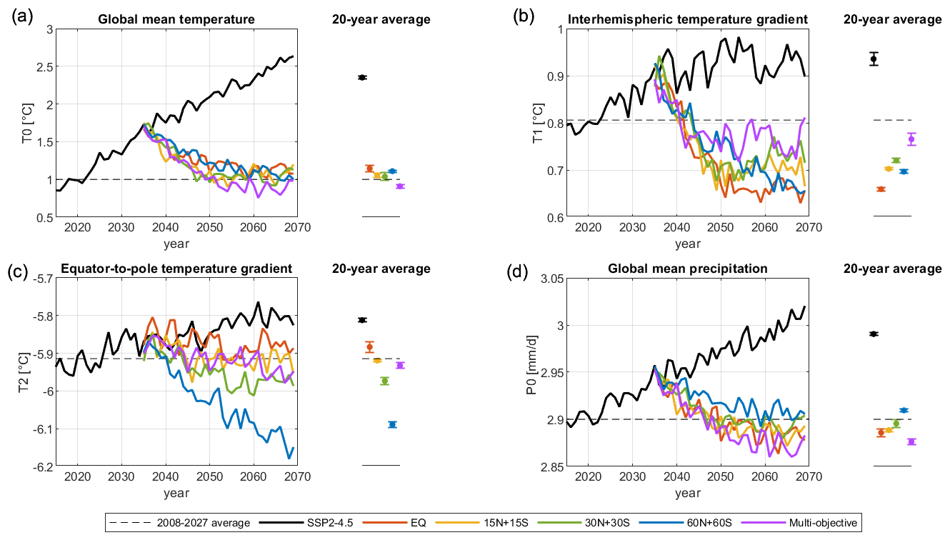
Figure 1Time evolution of (a) global mean surface temperature relative to the pre-industrial level (T0), (b) interhemispheric temperature gradient (T1), (c) Equator-to-pole temperature gradient (T2), and (d) global mean precipitation (P0). Each solid line represents the ensemble mean of each injection strategy. The dashed line represents the 20-year average during the reference period (2008–2027). The dots on the right of each panel represent the 20-year average over 2050–2069; the uncertainties in the calculated 20-year averages are estimated by ±1 standard error and represented by the error bars.
Without SAI, T1 increases over time under climate change (Fig. 1b) due to various reasons, such as differences in land cover, tropospheric aerosol, and heat capacity between the two hemispheres (Chiang and Friedman, 2012). We find that all SAI strategies considered here overcompensate T1, which corresponds to a reduction in temperature gradient between the NH and SH compared to the reference period (this includes the multi-objective case that targets T1, although that case has the smallest overcompensation). The overcompensation of T1 is likely linked to the reduction in cloud cover in the SH subtropics due to the strong cloud response to elevated CO2 levels in the SH in CESM2(WACCM6) (Fasullo and Richter, 2023). As a result, greater radiative heating needs to be mitigated in the SH. The same SAI strategies do not overcompensate T1 in other models. For example, in CESM1(WACCM), the equatorial injection, which yields slightly larger AOD in the NH than the SH, roughly maintained T1, as described in Kravitz et al. (2019). With greater radiative heating needed to be mitigated in the SH in CESM2(WACCM6) compared to CESM1(WACCM), the equatorial injection ends up overcompensating T1 in this model.
Figure 1c shows the evolution of the Equator-to-pole temperature gradient. T2 increases over time under SSP2-4.5 as the result of the warming being much faster in the Arctic than in the mid- and low latitudes. All SAI strategies considered here reduce T2 compared to the SSP2-4.5 simulation. The strategies injecting further poleward i.e., 30N+30S and 60N+60S, overcompensate T2 compared to the reference period, while the equatorial case undercompensates it. Some intuition for this is based on the observation that the radiative forcing from CO2 is roughly uniform with latitude, while insolation is higher in the tropics than towards the poles. Thus, one would expect a spatially uniform AOD to overcool the tropics relative to high latitudes, overcompensating T2. Injecting further poleward increases AOD further poleward, and in this model, injecting at 15N and 15S is roughly sufficient to balance the mismatch between the spatial distribution of radiative forcing from CO2 and that of sunlight, and thus to simultaneously balance T0 and T2 – essentially giving the latter for free, while only directly controlling for T0. A more complete description would depend on other factors, including details of the stratospheric circulation, and the rapid cloud adjustment to CO2 forcing noted in Fasullo and Richter (2023); as a result, the specific injection latitudes that would simultaneously balance both T0 and T2 will be model dependent.
Figure 1d shows the evolution of global mean precipitation. With increasing greenhouse gas (GHG) forcing, global mean precipitation increases over time in the SSP2-4.5 simulation. This response has been observed under rising GHG levels across climate models (IPCC, 2021) and arises because global mean precipitation is governed by the availability of energy (Allen and Ingram, 2002; O'Gorman et al., 2012). With the added SAI forcing, the global mean precipitation is reduced, consistent with the associated decrease in global mean temperature and is overcompensated relative to the global mean precipitation in the reference period (P0=2.9 mm d−1), except for the 60N+60S case. This overcompensation in precipitation relative to the associated decrease in temperature was observed in many previous studies using either solar reduction (Bala et al., 2008; Tilmes et al., 2013) or stratospheric aerosols (Niemeier et al., 2013; Lee et al., 2020).
To understand what factors affect the overcompensation of global mean precipitation, we use the precipitation and temperature data from the five SAI strategies, as well as SSP2-4.5, to calculate the hydrological sensitivity (the slope between global mean precipitation and global mean surface air temperature) under different SAI strategies. The results in Fig. 2 show that the hydrological sensitivity is dependent on the injection latitude; injecting SO2 at lower latitudes yields a stronger reduction in the global mean precipitation per unit of reduction in global mean temperature, as shown in Fig. 2a. EQ has the strongest reduction in precipitation per unit of global cooling, followed by 15N+15S, multi-objective, and 30N+30S; the 60N+60S strategy has the least reduction in precipitation per unit of global cooling. This dependence on the injection latitude is also observed in the tropical region; injecting at lower latitudes yields a stronger reduction in the tropical mean precipitation per unit of reduction in tropical mean temperature (Fig. 2b). It is likely that tropical cooling has a comparatively larger impact on global mean precipitation compared to the surface cooling that occurs outside the tropics, so the strategies with stronger tropical cooling yield stronger overcompensation in global mean precipitation (Fig. 2). In addition, the increase in tropospheric static stability as the result of aerosol-induced lower-stratospheric heating can also contribute to the reduction in the global mean precipitation (Simpson et al., 2019).
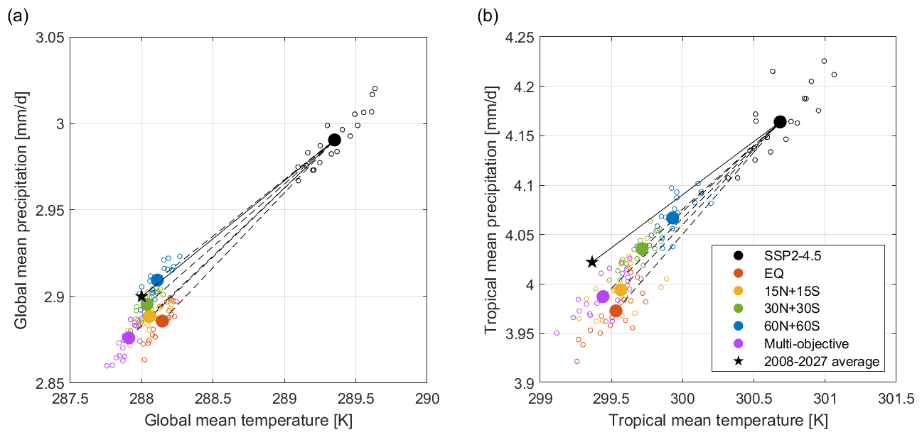
Figure 2A comparison (a) between the global mean temperature and global mean precipitation and (b) between the tropical mean temperature and tropical mean precipitation. The tropical means are calculated over the region between 20° N and 20° S. All data shown here are ensemble means. Small hollow dots represent the annual means from 2050–2069 under SSP2-4.5 or a given SAI strategy, and large solid dots represent the 20-year average over 2050–2069. The black star represents the 20-year average of temperature and precipitation from the reference period (2008–2027). The slope of the solid lines represents the increase in precipitation per unit of warming under GHG forcing. The slope of the dashed lines represents the precipitation reduction per unit of cooling under SAI forcing. The change in precipitation shows a strong dependence on injection latitude; injecting at lower latitudes yields a stronger reduction in the global mean precipitation per unit of global cooling and a stronger reduction in the tropical mean precipitation per unit of tropical cooling.
4.2 Injection rates and AOD
Figure 3 shows the evolution of the total SO2 injection rate in each SAI strategy (Fig. 3a) and the 20-year (2050–2069) average injection rates (Fig. 3b). Even though all five injection strategies aim to maintain the global mean surface temperatures at the same levels, different amounts of SO2 injections are required in each case to achieve this. Among the five strategies, the 30N+30S strategy requires the least amount of injection, and the EQ and 60N+60S strategies require the largest amount of injection, which are, respectively, 59 % and 50 % more than the injection required by the 30N+30S strategy. The multi-objective strategy injects the majority (nearly two-thirds) of the SO2 in the Southern Hemisphere (Fig. 3b); the average injection rate during 2050–2069 at 30° S, 15° S, 15° N, and 30° N is 2.4, 8.8, 5.1, and 0.7 Tg yr−1, respectively. This hemispheric asymmetry in the distribution of SO2 injections is not due to the Brewer–Dobson circulation, as the interhemispheric imbalance for zonal mean AOD, ℓ1, under the hemispherically symmetric strategies is much smaller than the value of ℓ1 that is needed by the multi-objective strategy to compensate for T1. It is likely due to the rapid cloud responses to elevated CO2 levels in CESM2(WACCM6), which results in greater radiative heating that needs to be mitigated in the SH (Fasullo and Richter, 2023).
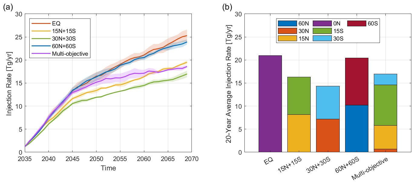
Figure 3(a) Total amount of SO2 injected into the stratosphere per year (Tg yr−1), and (b) annual injection of SO2 (Tg yr−1) at each latitude averaged over the last 20 years (2050–2069) for each SAI strategy. The solid lines in panel (a) represent the mean injection rate of each strategy, which is averaged over three ensemble members; the width of the shading represents the standard error in the injection rates across ensemble members for each SAI strategy. The 20-year (2050–2069) average injection rates of EQ, 15N+15S, 30N+30S, 60N+60S, and multi-objective strategies are 21, 16, 14, 20, and 17 Tg yr−1, respectively.
The efficiency of AOD and of global mean surface cooling per unit injection for these five strategies is shown in Fig. 4a and c, respectively. These results indicate that it is more efficient in terms of cooling per unit injection to inject SO2 in mid-latitudes than in the tropics or high latitudes. The low efficiency in the equatorial injection is partially due to larger aerosol particles being formed near the tropics, as the aerosols are relatively confined inside the tropical pipe and, hence, more prone to coagulation and condensation (Fig. 5b; see also Visioni et al., 2017; Kravitz et al., 2019). The relatively larger aerosol effective radius in the equatorial injection case notably reduces the AOD per unit mass of sulfate and also slightly reduces the aerosol lifetime in the stratosphere due to increased sedimentation. This results in the strongest increase in stratospheric water vapor which, as a greenhouse gas, offsets some of the direct aerosol cooling (Visioni et al., 2021; Bednarz et al., 2023c); this effect thus requires increased SO2 injection rates to compensate.
The notably lower efficiency of AOD per unit of injection in the 60N+60S strategy is because aerosols injected at high latitudes have a much shorter lifetime due to the proximity to the downward branch of the stratospheric Brewer–Dobson circulation and stratosphere–troposphere exchange areas, thus resulting in faster transport to the troposphere where they are removed (Butchart, 2014; Lee et al., 2021; Visioni et al., 2023a). The average lifetime of the injected stratospheric aerosol (calculated as the ratio of stratospheric SO2 burden to injection rate) is 1.36 ± 0.009, 1.39 ± 0.011, 1.26 ± 0.010, and 0.58 ± 0.004 years for the strategies EQ, 15N+15S, 30N+30S, and 60N+60S, respectively. Although 60N+60S has the lowest efficiency of AOD per unit injection, it yields the highest efficiency of global cooling per unit of global mean AOD (Figs. 4a–b, 5a), due to its strong effectiveness in offsetting Arctic amplification (Zhao et al., 2021; see also Sect. 4.1), as the initial cooling from high-latitude AOD is amplified by the high-latitude feedbacks (Holland and Bitz, 2003; Serreze and Barry, 2011; Hahn et al., 2021; Previdi et al., 2021). Figure 4b also indicates that the efficiency of global cooling per unit AOD increases with latitude.
Nonlinearity is observed in the efficiency of AOD per unit injection, which is more notable in the low- and mid-latitude injections (Fig. 5a). Higher concentration of SO2 in the stratosphere results in larger aerosol particles which in turn sediment out faster, thus leading to smaller AOD per unit mass of sulfate (Niemeier and Timmreck, 2015; Kleinschmitt et al., 2018; Visioni et al., 2020a). Compared to high-latitude injection, low- and mid-latitude injections result in larger aerosol effective radius (Fig. 5b).
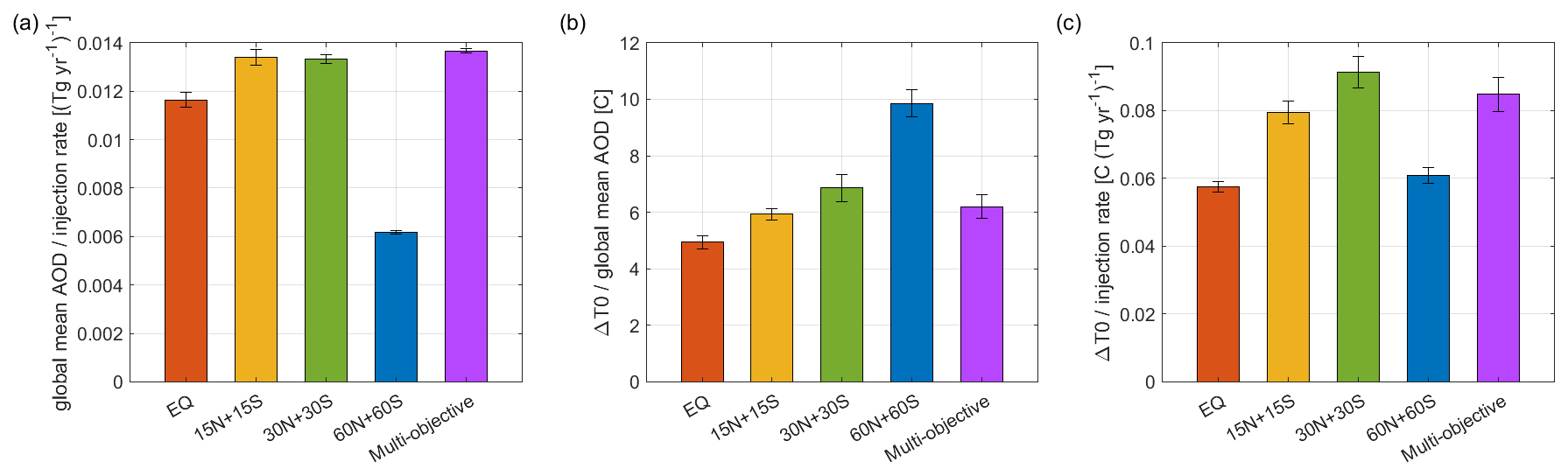
Figure 4(a) Global mean AOD per unit of the injection rate (), (b) global cooling per unit of global mean AOD (C), and (c) global cooling per unit of injection rate () calculated over the 20-year period of 2050–2069. Error bars represent the standard error of the mean.
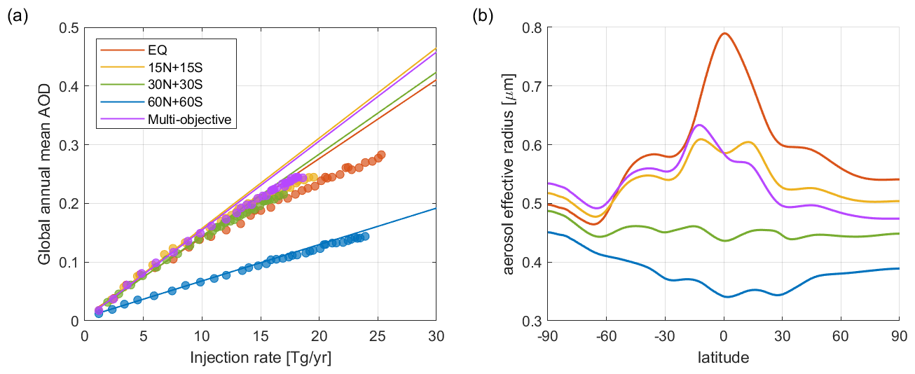
Figure 5(a) The relationship between the injection rate and corresponding global mean AOD in each year of each simulation and (b) the latitudinal distribution of concentration-weighted aerosol effective radius in the stratosphere, averaged over the last 20 years (2050–2069). The lines in panel (a) are linear fits under low injection rates (i.e., when the injection rate is lower than 10 Tg yr−1).
Figure 6 shows the latitudinal distributions of the zonal mean AOD and zonal mean temperature changes for different SAI strategies, averaged over the last 20 years of the simulations (2050–2069). Injecting in the tropics yields an asymmetrical AOD distribution between hemispheres, with higher AOD in the NH and lower AOD in the SH. This asymmetry arises as the Northern Hemisphere has a stronger Brewer–Dobson circulation than the Southern Hemisphere (Butchart, 2014). In contrast, injecting in the extratropics results in a relatively hemispherically symmetric distribution of AOD. With the multi-objective strategy, AOD in the SH is notably higher than the NH, consistent with the largest injection rates at 15° S (Richter et al., 2022) that are required to minimize changes in the interhemispheric surface temperature gradient (Fig. 6b). Although the hemispherically symmetric strategies yield similar levels of AOD at high latitudes in both hemispheres, the cooling in the Arctic is much larger than in the Antarctic (Fig. 6b–c), due to polar amplification asymmetry (Salzmann, 2017).
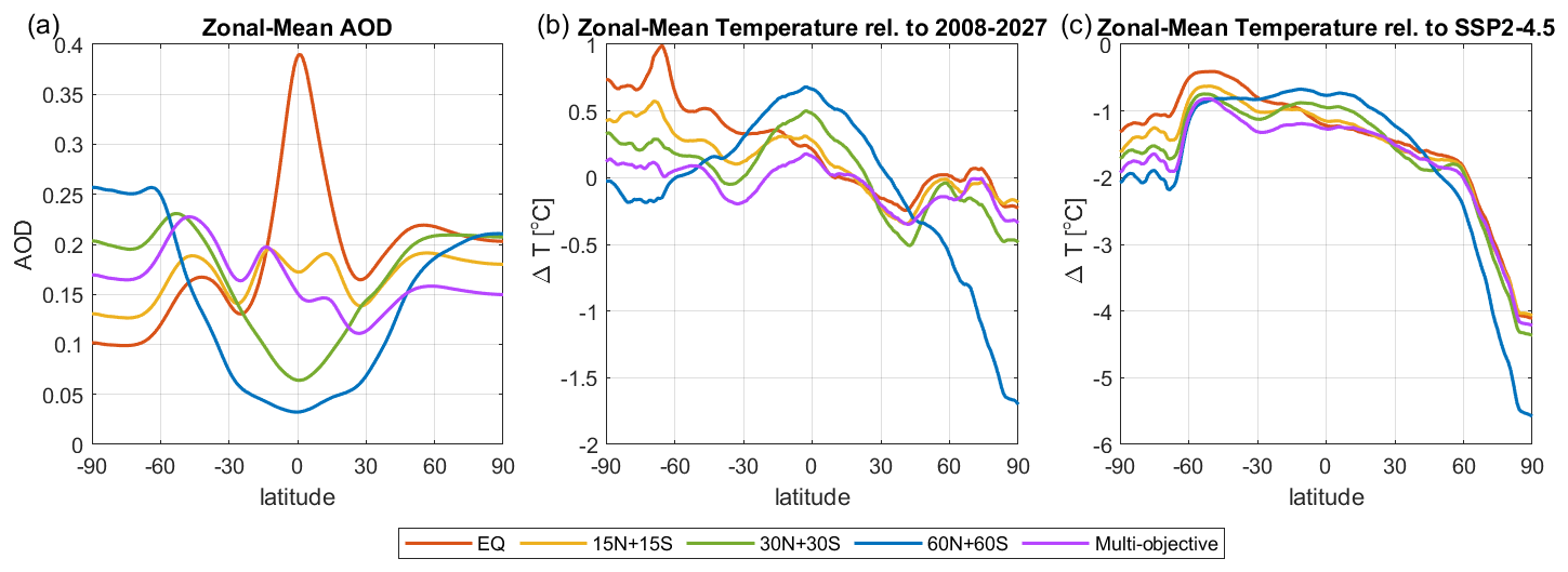
Figure 6Latitudinal distribution of (a) zonal mean AOD per degree Celsius of global cooling, (b) zonal mean surface air temperature response relative to the 20-year average of the reference period, 2008–2027, and (c) zonal mean surface air temperature response relative to the same 20-year period (2050–2069) under the SSP2-4.5 scenario.
Figure 7 shows the spatiotemporal distribution of stratospheric AOD for all five SAI strategies. We normalize the values of AOD by the associated amount of global mean cooling under each SAI strategy. The simulated distribution of AOD depends on the latitudinal transport of air toward the poles, which is affected by both the seasonality in the Brewer–Dobson circulation and the strength of the stratospheric polar vortex (Visioni et al., 2020a). The distribution of AOD in the annual injection cases exhibits a marked seasonal cycle, with extratropical AOD maximizing in winter and spring at each hemisphere, due to seasonality in the strength of the stratospheric transport. In the case of the high-latitude seasonal injections, AOD maximizes in the mid- and high latitudes in the season following the season of SO2 injections because it takes about 1 month for injected SO2 to oxidize into aerosols (Lee et al., 2021).
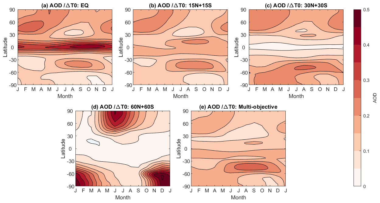
Figure 7Simulated seasonal cycle of AOD at each latitude for 1 °C of global mean cooling under each SAI injection strategy.
4.3 Surface air temperature, precipitation, and P−E
Section 4.1–4.2 focused on the large-scale global responses to different SAI strategies; we now evaluate the corresponding changes in regional surface climate over the whole Earth surface. We average the annual mean surface air temperatures, precipitation, and precipitation minus evaporation (P−E) over the 2050–2069 period and all three ensemble members and calculate the changes relative to the reference period (2008–2027). We perform Welch's t test on the ensemble mean of the annual mean temperature, precipitation, and P−E during the year 2050–2069 to evaluate whether these regional changes are statistically significant. Since this test assumes that sampled data are independent, we perform the t tests using the estimated effective sample size by assuming that temperatures, precipitation, and P−E all follow a first-order autoregressive (AR(1)) process (Wilks, 2019) and perform multiple testing correction on the t test results to account for spatial correlation using the FDR method. We also evaluate how well these strategies compensate for the regional changes under climate change by comparing the area-weighted root mean square (rms) change.
Figure 8 shows the simulated changes in surface air temperatures. In SSP2-4.5, most areas on the Earth are warmer than the reference period, with the largest warming found in the Arctic region due to Arctic amplification. Overall, the temperature increase over land is higher than over the ocean (Fig. 8a). The exception to the overall warming trend is a region in the North Atlantic Ocean, which shows a cooling pattern (so-called North Atlantic warming hole) that is related to the weakening of Atlantic meridional overturning circulation (AMOC) (see Tilmes et al., 2020 and Fasullo and Richter, 2023; see also Fig. 16). The North Atlantic warming hole has also shown up in simulations in other climate models (Chemke et al., 2020; Keil et al., 2020), as well as in the RCP8.5 scenario simulated in CESM1(WACCM) (Tilmes et al., 2017). In addition to the reduced northward heat transport due to the weakening of AMOC, the formation of the warming hole has been shown to be also driven by increased ocean heat transport from the warming hole to higher latitudes and a shortwave cloud feedback (Keil et al., 2020).
Figure 8b–f show that all SAI strategies effectively counteract the large-scale surface warming, as illustrated by the large fraction of surface area showing no statistically significant temperature difference relative to the reference climate. With SAI, the percentage of area with no statistically significant change ranges from 71 % to 84 %, while only 15 % of total area has no statistically significant difference without SAI. Despite similar magnitudes of global mean cooling (Fig. 1a), different SAI strategies yield different regional temperature responses. The EQ strategy undercools the Southern Hemisphere, which is due to greater radiative heating that needs to be mitigated in SH in CESM2(WACCM6) (Fasullo and Richter, 2023). In contrast, the 60N+60S strategy overcools the Arctic and undercools the tropics because the injections are focused at higher latitudes and the resulting aerosols are rapidly transported poleward and downward by the Brewer–Dobson circulation.
In all simulations (Fig. 8), the surface air temperature in a region in the North Atlantic Ocean is lower than the reference period, similar to the response found in the SSP2-4.5 simulation. This phenomenon is caused by the weakening of AMOC, which is discussed above and in more detail in Sect. 4.8. We also find consistent temperature changes over the Pacific Ocean across all SAI simulations and the SSP2-4.5 simulation, with relative warming in the eastern Pacific in both its equatorial and northern regions compared to the reference period, albeit differing in the strength and horizontal extent of the anomalous equatorial Pacific warming. The pattern is similar to the pattern associated with the positive phase of the El Niño–Southern Oscillation (ENSO; e.g., McGregor et al., 2022) and, as such, projects on changes in the ENSO index. This is associated with changes in the strength and the position of the Walker circulation (Bednarz et al., 2023a), contributing to the precipitation changes simulated in the Amazon region (Sect. 4.4). As pointed out in Visioni et al. (2023b), such changes are also dependent on the choices of the reference period against which we are comparing and are in part driven by an undercompensation of GHG warming.
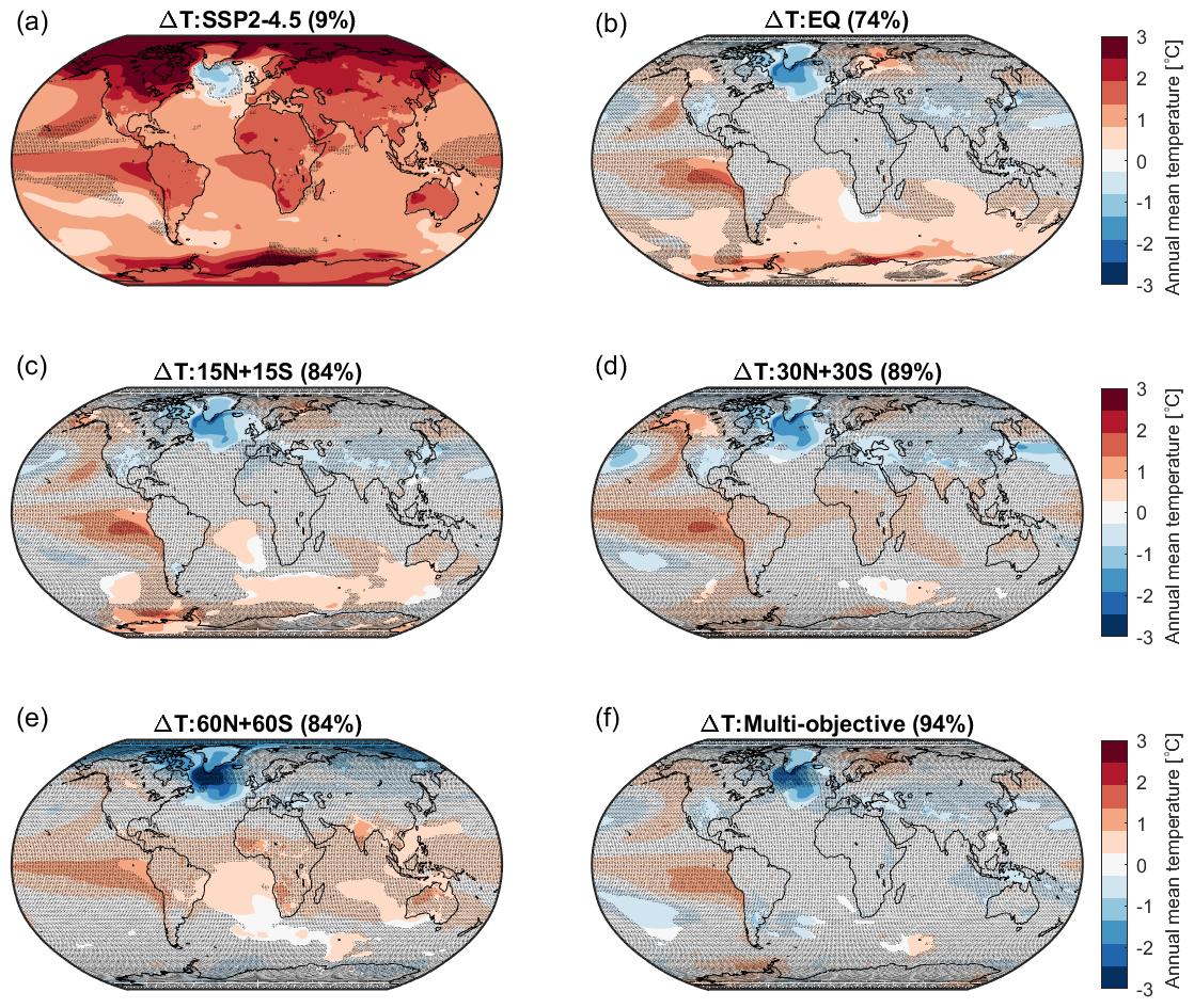
Figure 8Changes in surface air temperature, averaged over 2050–2069, compared to the reference period (2008–2027) for (a) SSP2-4.5 and (b–f) different SAI injection strategies. Shaded areas indicate where the change relative to the reference period is not statistically significant, based on a two-tailed Welch's t test, with a confidence level of 95 %. The percentage of area with no statistically significant change in surface air temperature is listed in the title of each map.
Figure 9 shows the simulated changes in precipitation. Under the SSP2-4.5 scenario, about 43 % of the area has a statistically significant change in precipitation compared to the reference period (Fig. 9a). While the percentage of area with statistically significant change in precipitation (27 %–38 %) is slightly reduced by SAI, SSP2-4.5 and SAI scenarios share similar spatial patterns of changes in precipitation. In particular, among SSP2-4.5 and all SAI cases, the most significant change occurs in the equatorial Pacific Ocean and follows a similar pattern – i.e., precipitation decreases in the northern region and increases in the southern region. This corresponds to the Intertropical Convergence Zone (ITCZ) shifts discussed in Sect. 4.5 and the fact that none of the SAI strategies manages to fully offset the southward ITCZ shift simulated in SSP2-4.5.
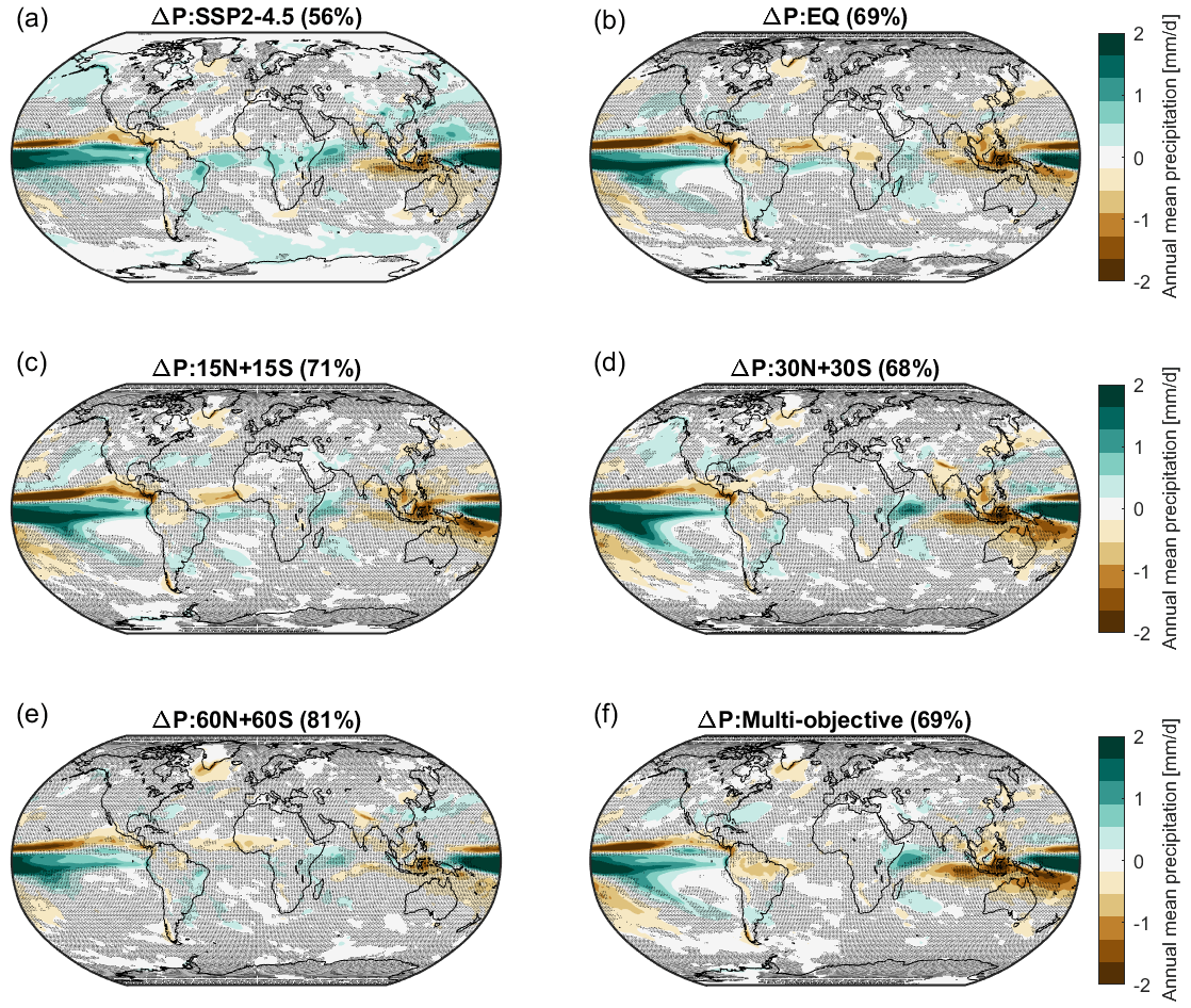
Figure 9Changes in precipitation averaged over 2050–2069, compared to the reference period (2008–2027) for (a) SSP2-4.5 and (b–f) different SAI injection strategies. Shaded areas indicate where the response is not statistically significant based on a two-tailed Welch's t test with a confidence level of 95 %. The percentage of area with no statistically significant change in precipitation is listed in the title of each map.
The net flux of water from the atmosphere to the Earth's surface is described by precipitation minus evaporation (P−E). Figure 10 shows the simulated changes in P−E over land. Under the SSP2-4.5 scenario, 33 % of the land area has a statistically significant change in P−E compared to the reference period (Fig. 10a) and the percentage of land area with statistically significant change in P−E is slightly reduced by SAI (Fig. 10b–f). While the SAI scenarios have roughly the same percentage of the land area with statistically significant change in P−E (20 %–27 %), the regional changes in P−E vary between the different SAI strategies, as well as the SSP2-4.5 run (Fig. 10). For example, the EQ strategy makes central Africa drier, while the P−E response in central Africa is not statistically significant under other SAI strategies. Also, the reduction in P−E over north India is statistically significant under 30N+30S and 60N+60S strategies but not statistically significant under the other strategies.
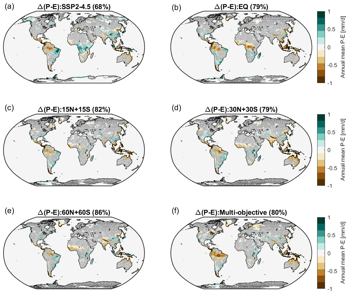
Figure 10Changes in precipitation minus evaporation (P−E) over land averaged over 2050–2069, compared to the reference period (2008–2027) for (a) SSP2-4.5 and (b–f) different SAI injection strategies. Shaded areas indicate where the response is not statistically significant based on a two-tailed Welch's t test with a confidence level of 95 %. The percentage of land area with no statistically significant change in P−E is listed in the title of each map.
To evaluate how well these strategies compensate for the change in regional temperature, precipitation, and P−E over land under climate change, we calculate an ensemble mean area-weighted rms change comparing the 2050–2069 average to the reference period (Fig. 11a). We also calculate the rms change due to natural variability alone. This is done by first detrending the annual mean over 2008–2027 at each grid box in the three ensemble members and then calculating the area-weighted rms standard error of the processed data, assuming an AR(1) autocorrelation process. If an SAI strategy fully compensates the GHG-induced regional changes, then on average the rms response will be similar to the rms change due to natural variability alone. However, we find that in all SAI strategies, the rms temperature change is larger than the rms temperature change that one would expect due to natural variability alone (i.e., 0.15 °C, represented by the dashed line in Fig. 11a), indicating imperfect compensation of the pattern of warming under climate change. Among the SAI strategies considered here, the multi-objective strategy best minimizes the spatial rms of temperature changes, as indicated by the lowest rms temperature change (rms T=0.38 °C). The 60N+60S strategy results in an uneven cooling with the highest rms temperature change (rms T=0.57 °C) but still much smaller than the rms temperature change in SSP2-4.5 without SAI (rms T=1.53 °C). All SAI strategies give rise to mean rms precipitation and P−E responses that are larger than those from natural variability alone (which are estimated as approximately 0.16 and 0.10 mm d−1 for precipitation and P−E changes, respectively; Fig. 11b–c). The difference in the spatial rms of precipitation and P−E responses between SAI simulations and the SSP2-4.5 simulation is notably smaller than the difference in rms temperature responses, indicating a poorer compensation of these metrics than temperature. When comparing any SAI strategy with the SSP2-4.5 case, the difference in rms precipitation response is no more than 30 % (Fig. 11b), and the difference in rms P−E response over land is no more than 12 % (Fig. 11c).
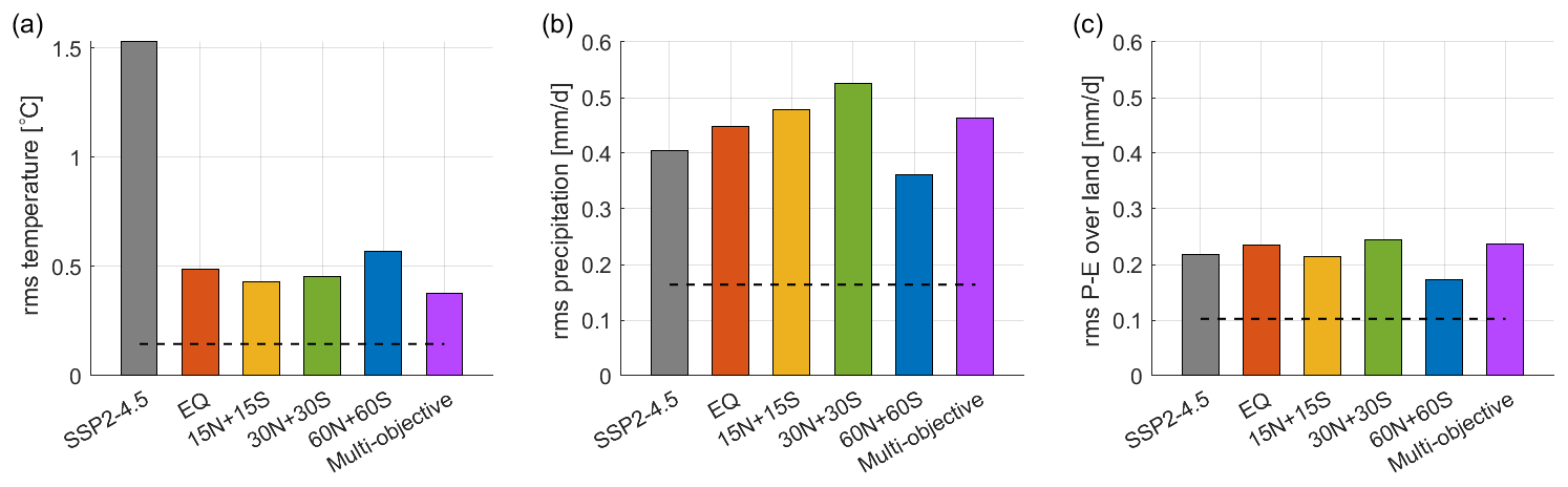
Figure 11Area-weighted root mean square deviation between the (a) temperature, (b) precipitation, and (c) P−E over land averaged over 2050–2069 and the reference period (2008–2027). The dashed lines represent the area-weighted root mean square of each quantity due to natural variability alone.
4.4 Precipitation change in Amazon and Congo basins
In this section, we focus on the Amazon and Congo basins in particular to show that different strategies have different impacts on regional precipitation. For the Amazon Basin, we average precipitation over the region between 5° N–15° S and 50° W–78° W (a total land area of 7.2×10⁶ km2). For the Congo Basin, we average temperature over the region between 8° N–10° S and 12–31° E (a total land area of 4.6×10⁶ km2). Precipitation changes in these tropical river basins have direct effects on local ecosystems. Rainforests in both regions act as carbon sinks and are thus of great importance to global climate. It is well studied that El Niño–Southern Oscillation (ENSO) is one of the main drivers of interannual variability in convective precipitation over the Amazon Basin (Marengo and Espinoza, 2016; Jiménez-Muñoz et al., 2016). Precipitation over the Amazon Basin is suppressed during El Niño events and enhanced during La Niña events (Marengo and Espinoza, 2016; Jiménez-Muñoz et al., 2016).
In the Amazon Basin, the 20-year average (2050–2069) under SSP2-4.5 is similar to the reference level (Fig. 12a), though with regional variations within the basin; the central region becomes drier, while the southeastern area gets wetter (see precipitation maps in Fig. S5). All SAI strategies result in a reduction in the mean precipitation, except for the 60N+60S case (which is not statistically significantly different from either the reference or the SSP2-4.5 case). The multi-objective strategy yields the strongest precipitation reduction. The hemispherically symmetric strategies show a dependence of the precipitation reduction on the latitude of injection, with the largest decrease in the Amazon Basin precipitation in EQ and no statistically significant decrease in 60N+60S. This pattern of precipitation changes is likely related to the corresponding changes in the intensity of the tropospheric Walker circulation and thus ENSO response, as also discussed in Bednarz et al. (2023a). We approximate the ENSO changes by calculating the ENSO index as a difference in near-surface air temperature between the Niño 3.4 region (5° N–5° S, 120–170° W) and all tropical oceans (20° N–20° S), based on the method described in van Oldenborgh et al. (2021). The strength of the Walker circulation is approximated by the difference in sea level pressure between the east Pacific Ocean (5° N–5° S, 80–160° W) and the Indian Ocean (5° N–5° S, 80–160° E), based on the method described in Kang et al. (2020). Figure S7 shows that changes in the Niño 3.4 index and the strength of Walker circulation both contribute to and partly explain the precipitation responses simulated across the different SAI strategies and the SSP2-4.5 simulation in the Amazon Basin, with the coefficient of determination (R2) of the best-fit linear regression functions equal to 0.62 and 0.66, respectively.
In the Congo Basin, the average precipitation in the SSP2-4.5 scenario increases over time (Fig. 12b), likely as the result of the intensification of the global hydrological cycle under increasing surface temperatures (Sect. 4.1). In contrast, all SAI strategies result in a reduction in the mean precipitation in the Congo Basin compared to the SSP2-4.5 case, as the global mean surface temperatures are reduced to around the reference level (Fig. 1a). While the multi-objective strategy brings the 20-year average (2050–2069) mean precipitation back to the reference level, other strategies either undercompensate or overcompensate the precipitation. The equatorial and 15N+15S injection strategies result in a statistically significant undercompensation of the Congo Basin precipitation compared to the reference period, while 30N+30S and 60N+60S result in a small overcompensation. The dependence of the precipitation reduction in the Congo Basin on the latitude of aerosol injection is partly indicative of the corresponding impacts from the intensity change in the tropospheric Hadley circulation. As shown in Bednarz et al. (2023a), Hadley circulation weakens significantly under EQ and 15N+15S strategies but stays unchanged for 30N+30S and 60N+60S; these tropospheric circulation changes could thus contribute to and partially explain the precipitation changes simulated in the Congo Basin across the strategies.
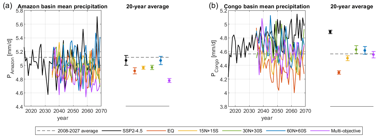
Figure 12Time evolution of mean precipitation in (a) Amazon Basin and (b) Congo Basin. Each solid line represents the ensemble mean of each injection strategy. The dashed line represents the 20-year average during the reference period (2008–2027). The dots on the right of each panel represent the 20-year average over 2050–2069; the uncertainties in the calculated 20-year averages are estimated by ±1 standard error and represented by the error bars.
4.5 Intertropical convergence zone
The Intertropical Convergence Zone (ITCZ) is a region of heavy precipitation near the Equator, where the northeast and southeast trade winds collide (Byrne et al., 2018). Different metrics have been used in previous studies to define the ITCZ location, such those based on the precipitation centroid (e.g., Frierson and Hwang, 2012; Donohoe et al., 2013; Byrne et al., 2018; Lee et al., 2020) or based on atmospheric mass circulation (e.g., Hari et al., 2020; Cheng et al., 2022). Here, we define the ITCZ location as the latitude near the Equator, where the zonal mean meridional streamfunction at 500 hPa changes sign. The streamfunction at each latitude is calculated using the following equation:
where [v] is the zonal mean meridional velocity, a is the Earth's radius, ϕ is latitude, and p is 500 hPa. The ITCZ location is approximated using a linear interpolation of the centers of two consecutive grid cells that have meridional circulations of opposite directions.
Under GHG forcing alone, the latitude of ITCZ shifts southward from its location in the reference period (Fig. 13a). All hemispherically symmetric SAI injection strategies shift the latitude of the ITCZ further south, consistent with the stronger associated cooling in the NH than in the SH (Fig. 6b–c). The difference in the shift in the ITCZ between the hemispherically symmetric injection cases is modest, generally within 1 standard error. The multi-objective strategy, on the other hand, shifts the latitude of ITCZ northward from that due to GHGs alone, but it is still south of the ITCZ position in the reference period. The multi-objective strategy is the only one that explicitly targets hemispheric asymmetry; while T1 is an imperfect proxy for managing ITCZ, it does result in improved compensation relative to the hemispherically symmetric strategies, indicating the value of including an objective associated with asymmetric compensation.
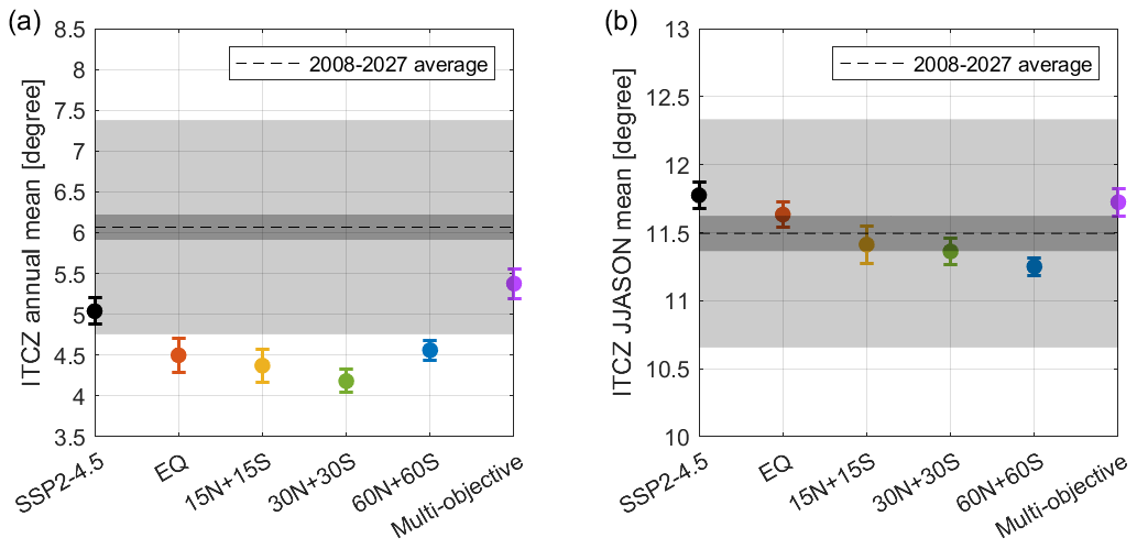
Figure 13The 20-year (2050–2069) average (dots) and standard error (vertical bars) of the (a) annual mean and (b) seasonal mean (June through November, JJASON) latitude of ITCZ for SSP2-4.5 and the different SAI strategies. The dashed horizontal line represents the mean latitude of ITCZ during the reference period (2008–2027), and the shaded areas represent the corresponding standard error (dark gray) and standard deviation (light gray).
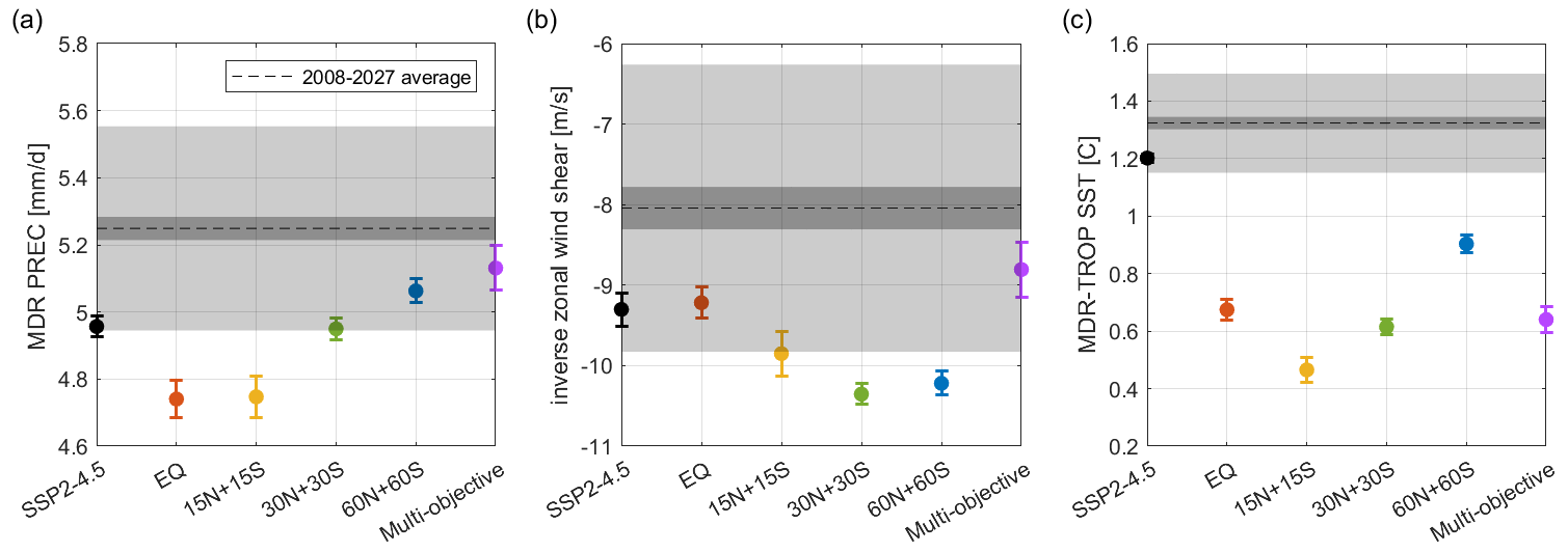
4.6 Tropical cyclone frequency
Existing studies show that climate change will decrease the overall tropical cyclone (TC) frequency but increase the frequency of the most intense ones (Bengtsson et al., 2007; Knutson et al., 2010; Camargo, 2013). Figure 14 evaluates the North Atlantic TC activity based on three TC indices that are described in Dunstone et al. (2013) and Jones et al. (2017). These TC indices evaluate the average precipitation in the main development region (MDR; defined as 5–20° N and 15–85° W), the inverse vertical zonal wind shear between 850 and 250 hPa in the MDR, and the sea surface temperature (SST) difference between the MDR and the tropics as a whole. All three indices are calculated for the hurricane season in the North Atlantic, which is June–November (JJASON). An increase in MDR precipitation, inverse vertical zonal wind shear, or the relative SST indicates an increase in TC frequency.
We find that all three TC indices show reduction in TC frequency under SSP2-4.5 (Fig. 14), in agreement with the existing literature (Bengtsson et al., 2007; Knutson et al., 2010; Camargo, 2013). TC frequency also decreases with SAI deployment, but the magnitude of the reduction in TC frequency under different SAI strategies varies among the different TC metrics. In general, lower-latitude injections tend to have a larger reduction in the average MDR precipitation (Fig. 9), which yields a larger reduction in TC frequency compared to SSP2-4.5 or the higher-latitude injections (Fig. 14a). However, Fig. 14b shows that lower-latitude injections result in a smaller increase in the zonal wind shear, which yields a smaller reduction in TC frequency compared to higher-latitude injections. The relative change in the inverse zonal wind shear between different SAI strategies is generally consistent with the relative change in ITCZ location in JJASON (Fig. 13b), as a southward shift in the ITCZ is related to an increase in zonal wind shear over the MDR (Dunstone et al., 2013). For the SST-based TC metric, we find that all SAI strategies result in substantially stronger reduction in TC frequency than those caused by climate change alone (Fig. 14c). The magnitude of the SST-based TC response in the geoengineering runs is smallest for the 60N+60S SAI strategy.
4.7 Arctic sea ice
The Arctic sea ice extent is expected to decrease in response to increasing global warming. If the current emissions of 40 Gt yr−1 CO2 continue without reduction, the Arctic Ocean is very likely to become ice-free during summer before mid-century (Notz and Stroeve, 2018). The effectiveness of restoring Arctic sea ice through stratospheric aerosol injection is evaluated through comparing the predicted Arctic September sea ice extent (SSI) under SAI strategies and the SSP2-4.5 scenario. Figure 15a shows that all these five SAI strategies increase SSI to at least the reference period level by the year 2069. After around the year 2050, SSI starts to stabilize around the reference period level in the low- and mid-latitude injection cases, while SSI continues increasing in the high-latitude injection case; the latter is consistent with the associated surface temperature changes (Fig. 8) and their Equator-to-pole gradients (Fig. 1c). The 60N+60S strategy increases SSI by the highest amount; the 20-year (2050–2069) average of SSI is about 5×10⁶ km2, which is 1.4×10⁶ km2 more than the reference period level. The overcompensation of SSI in the 60N+60S strategy is mainly because of the largest fraction of aerosols found in the polar region.
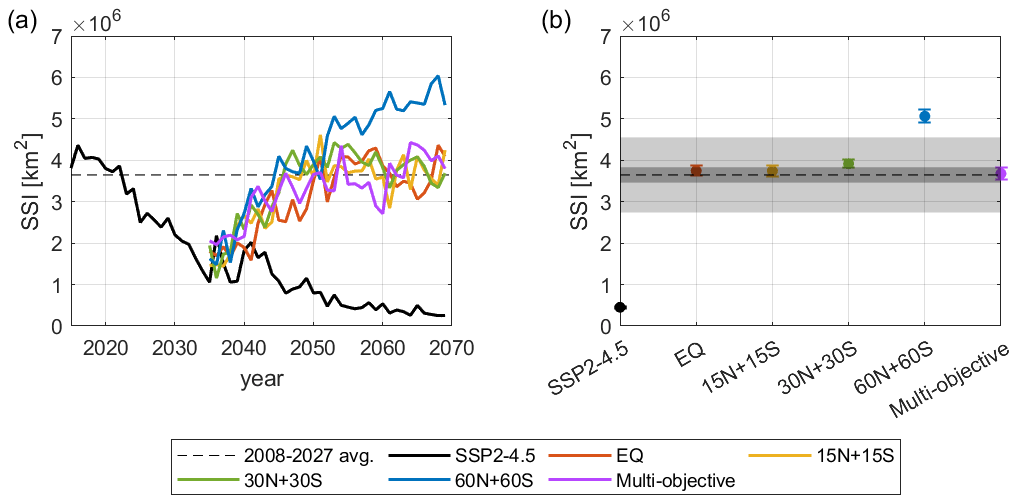
Figure 15(a) Time evolution of Arctic September sea ice extent (SSI) for SSP2-4.5 and the different SAI strategies. (b) The 20-year (2050–2069) average (dots) and standard error (vertical bars) of SSI for SSP2-4.5 and the different SAI strategies. The dashed horizontal line represents the average SSI during the reference period (2008–2027) and the shaded areas represent the corresponding standard error (dark gray) and standard deviation (light gray).
4.8 Atlantic meridional overturning circulation
Section 4.3 and Fig. 8 show that all simulations yield a region in the North Atlantic Ocean that is cooler than the reference period. Accordingly, Fig. 16a shows that in CESM2(WACCM6), AMOC continues to weaken over the 21st century under SSP2-4.5, which is consistent with the predictions from other climate models (Chemke et al., 2020; Keil et al., 2020; IPCC, 2021). AMOC moves warm water northward at the surface from the tropics and cold water southward at the bottom of the ocean from the North Atlantic (Rahmstorf, 2002). As AMOC weakens, less heat is transported northward to the North Atlantic, which causes the decrease in the surface air temperature over that region (Danabasoglu, 2008).
We find that low- and mid-latitude injections are better at recovering AMOC than the high-latitude injections. While the low- and mid-latitude injections do not restore AMOC back to the reference period, they do prevent further weakening of AMOC and keep AMOC at a strength similar to that in the year 2035 when injections are started. In comparison, AMOC continues weakening under the high-latitude SAI strategy but at a much lower rate compared to the SSP2-4.5 case. The weakening of AMOC relative to the reference period is likely the main cause of the consistent cooling pattern over the North Atlantic in every strategy in Fig. 8.
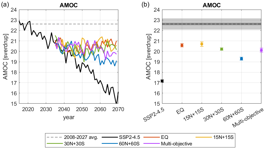
Figure 16(a) Time evolution of the strength of the Atlantic meridional overturning circulation (AMOC) under different SAI injection strategies over the period of 2035–2069, calculated as the maximum over the depth and latitude of the meridional streamfunction in the North Atlantic. (b) As in Fig. 11b but for the strength of the AMOC.
The question of whether to deploy SAI requires not just one simple answer but a series of deliberate decisions, including decisions on how much cooling to provide, what other climate objectives to achieve, and how to achieve them. Understanding the differences in surface climate responses between different injection strategies is crucial for making informed decisions.
In this work, we have considered a set of five SAI strategies under the same climate and SAI scenario to explore the range of possible climate responses in one climate model. These include four hemispherically symmetric injection strategies designed to maintain global mean temperature and one multi-objective strategy designed to maintain not only the global mean temperature but also the large-scale horizontal temperature gradients. The four hemispherically symmetric strategies are SO2 injection at the Equator, and injections of equal SO2 amounts at 15° N and 15° S, at 30° N and 30° S, and at 60° N and 60° S, with the latter only during spring in each hemisphere.
The choice of SAI strategies notably affects the spatiotemporal distribution of aerosol optical depths (AODs) and injection efficiencies and ultimately various surface climate responses. Injecting SO2 in the mid-latitudes provides more cooling per unit of injection than injecting in either the tropics or high latitudes. The low efficiency in the equatorial injection is primarily due to larger sizes of aerosols formed. The low efficiency in the high-latitude injection case is due to the aerosols having a much shorter lifetime. On the other hand, the 60N+60S case yields the highest global cooling per unit of global mean AOD.
We find that while all of these five SAI strategies maintain the global mean temperature at the reference level, they also overcompensate the interhemispheric temperature gradient. The amount of reduction in the Equator-to-pole temperature gradient depends on the choice of SAI strategy, with the high-latitude strategy yielding most reduction. In addition, all strategies overcompensate global mean precipitation, except the 60N+60S case. This is because injecting at lower latitudes results in stronger tropical cooling and more stratospheric heating, both of which lead to more reduction in precipitation.
Compared to the SSP2-4.5 case, all SAI strategies effectively reduce the percentage of area with statistically significant changes in temperature relative to the quasi present-day reference period, as well as the area-weighted root mean square (rms) change in regional temperature. In contrast, SAI strategies do not consistently reduce the rms change in precipitation minus evaporation (P−E) over land or the rms precipitation changes; the 15N+15S and 60N+60S strategies decrease the rms P−E change over land, while the other strategies slightly increase it.
The results show that while all SAI simulations reduce the weakening of the Atlantic meridional overturning circulation that is otherwise found for SSP2-4.5, they also fail to restore it back to the reference period level. Regarding the Arctic September sea ice extent (SSI), all SAI strategies restore SSI back to the reference period level, except the high-latitude injection strategy, which overcompensates SSI. The responses in the location of intertropical convergence zone and tropical cyclone frequencies vary among different SAI strategies.
Assessing the possible outcomes of SAI requires a good understanding of the possible impact from both the scenario and the choice of injection strategy. MacMartin et al. (2022) and Visioni et al. (2023b) have explored how different scenarios affect the climate responses to the same SAI strategy. In this work, we have demonstrated that different SAI strategies with similar objectives and under the same scenario would also affect the surface climate differently, with different distributions of outcomes. The study of these two different dimensions in the SAI design space lays the foundation for understanding the fundamental limits of SAI. Future research will explore combinations of these strategies, along with additional single-latitude cases (Visioni et al., 2023a; Lee et al., 2023a) to identify an optimal strategy for a given set of climate goals, and assess the underlying trade-offs between different climate goals, as well as to conduct similar analyses in other climate models. Knowing the range of possible climate outcomes and the trade-offs will help in making informed decisions on future policy on SAI deployment. Ultimately, other factors besides climate outcomes are also needed to be considered when evaluating benefits and risks of SAI.
In addition, our study demonstrates that the multi-objective strategy (Kravitz et al., 2017; Tilmes et al., 2018; Richter et al., 2022) yields a smaller residual regional temperature response than the hemispherically symmetric strategies considered here. However, such a strategy requires adjusting injection rates across four different latitudes to manage multiple goals and can thus be challenging to implement across many climate models. Simpler hemispherically symmetric strategies would be easier to replicate in a large multi-model intercomparison; either the combined 15N+15S or 30N+30S case considered here may represent a reasonable trade-off between how well a strategy compensates for climate changes and the complexity of implementation in a climate model. Our study thus provides fundamental understanding of the differences in the resulting climate responses between the more complex multi-objective strategy and simpler hemispherically symmetric ones, and as such is directly important for designing and understanding future large inter-model intercomparisons, including the next (seventh) phase of the Geoengineering Model Intercomparison Project (GeoMIP).
It is important to note that all simulations considered here are conducted using a single climate model, namely CESM2(WACCM6). Different climate models yield different patterns of AOD and surface climate responses for the same injection strategy (Visioni et al., 2023a; Fasullo and Richter, 2023). Also, atmospheric and climate responses from strategies with different injection locations are subject to different model structural uncertainties (e.g., Visioni et al., 2023a; Bednarz et al., 2023b). Simulating the same set of injection strategies in different global climate models will thus be important for better characterizing the uncertainties. In addition, the current study uses only a limited number of climate metrics to compare the different SAI strategies; other aspects of climate that are not analyzed here (e.g., Antarctic ice sheets, permafrost carbon, sea level, and ozone) may provide additional insights regarding the benefits and risks of SAI.
Data for the new simulations presented in this study are available at https://doi.org/10.5281/zenodo.7545452 (Zhang et al., 2023). Data for multi-objective strategy (from Visioni, 2022) are available at https://doi.org/10.7298/xr82-sv86.
The supplement related to this article is available online at: https://doi.org/10.5194/esd-15-191-2024-supplement.
YZ conducted all analyses and wrote the paper, with editing from DGM, EMB, DV, and BK. YZ and DGM conceived the study, with input from all authors. EMB and DV assisted with conducting simulations.
At least one of the (co-)authors is a member of the editorial board of Earth System Dynamics. The peer-review process was guided by an independent editor, and the authors also have no other competing interests to declare.
Publisher’s note: Copernicus Publications remains neutral with regard to jurisdictional claims made in the text, published maps, institutional affiliations, or any other geographical representation in this paper. While Copernicus Publications makes every effort to include appropriate place names, the final responsibility lies with the authors.
This article is part of the special issue “Resolving uncertainties in solar geoengineering through multi-model and large-ensemble simulations (ACP/ESD inter-journal SI)”. It is not associated with a conference.
The authors would like to acknowledge high-performance computing support from Cheyenne (https://doi.org/10.5065/D6RX99HX), provided by the National Center for Atmospheric Research (NCAR)'s Computational and Information Systems Laboratory, sponsored by the National Science Foundation.
Support for Yan Zhang and Douglas G. MacMartin has been provided by the National Science Foundation (grant no. CBET-2038246). Support for Daniele Visioni and Ewa M. Bednarz have been provided by the Cornell Atkinson Center for a Sustainable Future. Ewa M. Bednarz was also supported by the National Oceanic and Atmospheric Administration (NOAA) cooperative agreement NA22OAR4320151 and the Earth's Radiative Budget initiative. Support for Ben Kravitz has been provided in part by the Indiana University Environmental Resilience Institute. The Pacific Northwest National Laboratory is operated for the U.S. Department of Energy by the Battelle Memorial Institute (contract no. DEAC05-76RL01830). The Community Earth System Model (CESM) project is supported primarily by the National Science Foundation.
This paper was edited by Gabriele Messori and reviewed by three anonymous referees.
Allen, M. R. and Ingram, W. J.: Constraints on future changes in climate and the hydrological cycle, Nature, 419, 224–232, https://doi.org/10.1038/nature01092, 2002. a
Anderson, K., Broderick, J., and Stoddard, I.: A factor of two: how the mitigation plans of “climate progressive” nations fall far short of Paris-compliant pathways, Clim. Policy, 20, 1290–1304, https://doi.org/10.1080/14693062.2020.1728209, 2020. a
Bala, G., Duffy, P. B., and Taylor, K. E.: Impact of geoengineering schemes on the global hydrological cycle, P. Natl. Acad. Sci. USA, 105, 7664–7669, https://doi.org/10.1073/pnas.0711648105, 2008. a
Bala, G., Caldeira, K., and Nemani, R.: Fast versus slow response in climate change: implications for the global hydrological cycle, Clim. Dynam., 35, 423–434, https://doi.org/10.1007/s00382-009-0583-y, 2010. a
Bamber, J. L., Oppenheimer, M., Kopp, R. E., Aspinall, W., and Cooke, R.: Ice sheet contributions to future sea-level rise from structured expert judgment, P. Natl. Acad. Sci. USA, 116, 11195–11200, https://doi.org/10.1073/pnas.1817205116, 2019. a
Bednarz, E. M., Visioni, D., Richter, J. H., Butler, A. H., and MacMartin, D. G.: Impact of the Latitude of Stratospheric Aerosol Injection on the Southern Annular Mode, Geophys. Res. Lett., 49, e2022GL100353, https://doi.org/10.1029/2022GL100353, 2022. a
Bednarz, E. M., Butler, A. H., Visioni, D., Zhang, Y., Kravitz, B., and MacMartin, D. G.: Injection strategy – a driver of atmospheric circulation and ozone response to stratospheric aerosol geoengineering, Atmos. Chem. Phys., 23, 13665–13684, https://doi.org/10.5194/acp-23-13665-2023, 2023a. a, b, c, d, e
Bednarz, E. M., Visioni, D., Kravitz, B., Jones, A., Haywood, J. M., Richter, J., MacMartin, D. G., and Braesicke, P.: Climate response to off-equatorial stratospheric sulfur injections in three Earth system models – Part 2: Stratospheric and free-tropospheric response, Atmos. Chem. Phys., 23, 687–709, https://doi.org/10.5194/acp-23-687-2023, 2023b. a
Bednarz, E. M., Visioni, D., Kravitz, B., Jones, A., Haywood, J. M., Richter, J., MacMartin, D. G., and Braesicke, P.: Climate response to off-equatorial stratospheric sulfur injections in three Earth system models – Part 2: Stratospheric and free-tropospheric response, Atmos. Chem. Phys., 23, 687–709, https://doi.org/10.5194/acp-23-687-2023, 2023c. a
Bengtsson, L., Hodges, K. I., and Esch, M.: Tropical cyclones in a T159 resolution global climate model: comparison with observations and re-analyses, Tellus A, 59, 396–416, https://doi.org/10.1111/j.1600-0870.2007.00236.x, 2007. a, b
Bittner, M., Schmidt, H., Timmreck, C., and Sienz, F.: Using a large ensemble of simulations to assess the Northern Hemisphere stratospheric dynamical response to tropical volcanic eruptions and its uncertainty, Geophys. Res. Lett., 43, 9324–9332, https://doi.org/10.1002/2016GL070587, 2016. a, b
Bjordal, J., Trude, S., Alterskjær, K., and Carlsen, T.: Equilibrium climate sensitivity above 5 °C plausible due to state-dependent cloud feedback, Nat. Geosci., 13, 718–721, https://doi.org/10.1038/s41561-020-00649-1, 2020. a
Burgess, M. G., Ritchie, J., Shapland, J., and Pielke, R.: IPCC baseline scenarios have over-projected CO2 emissions and economic growth, Environ. Res. Lett., 16, 014016, https://doi.org/10.1088/1748-9326/abcdd2, 2021. a
Butchart, N.: The Brewer-Dobson circulation, Rev. Geophys., 52, 157–184, https://doi.org/10.1002/2013RG000448, 2014. a, b
Byrne, M., Pendergrass, A., Rapp, A., and Wodzicki, K.: Response of the Intertropical Convergence Zone to Climate Change: Location, Width, and Strength, Current Climate Change Reports, 4, 355–370, https://doi.org/10.1007/s40641-018-0110-5, 2018. a, b
Camargo, S. J.: Global and Regional Aspects of Tropical Cyclone Activity in the CMIP5 Models, J. Climate, 26, 9880–9902, https://doi.org/10.1175/JCLI-D-12-00549.1, 2013. a, b
Chemke, R., Zanna, L., and Polvani, L. M.: Identifying a human signal in the North Atlantic warming hole, Nat. Commun., 11, 1540, https://doi.org/10.1038/s41467-020-15285-x, 2020. a, b
Cheng, W., MacMartin, D. G., Kravitz, B.and Visioni, D., Bednarz, E. M., Xu, Y., Luo, Y., Huang, L., Hu, Y., Staten, P. W., Hitchcock, P., Moore, J. C., Guo, A., and Deng, X.: Changes in Hadley circulation and intertropical convergence zone under strategic stratospheric aerosol geoengineering, npj Climate and Atmospheric Science, 5, 32, https://doi.org/10.1038/s41612-022-00254-6, 2022. a
Chiang, J. C. and Friedman, A. R.: Extratropical Cooling, Interhemispheric Thermal Gradients, and Tropical Climate Change, Annu. Rev. Earth Pl. Sc., 40, 383–412, https://doi.org/10.1146/annurev-earth-042711-105545, 2012. a
Danabasoglu, G.: On Multidecadal Variability of the Atlantic Meridional Overturning Circulation in the Community Climate System Model Version 3, J. Climate, 21, 5524–5544, https://doi.org/10.1175/2008JCLI2019.1, 2008. a
Danabasoglu, G., Lamarque, J.-F., Bacmeister, J., Bailey, D. A., DuVivier, A. K., Edwards, J., Emmons, L. K., Fasullo, J., Garcia, R., Gettelman, A., Hannay, C., Holland, M. M., Large, W. G., Lauritzen, P. H., Lawrence, D. M., Lenaerts, J. T. M., Lindsay, K., Lipscomb, W. H., Mills, M. J., Neale, R., Oleson, K. W., Otto-Bliesner, B., Phillips, A. S., Sacks, W., Tilmes, S., van Kampenhout, L., Vertenstein, M., Bertini, A., Dennis, J., Deser, C., Fischer, C., Fox-Kemper, B., Kay, J. E., Kinnison, D., Kushner, P. J., Larson, V. E., Long, M. C., Mickelson, S., Moore, J. K., Nienhouse, E., Polvani, L., Rasch, P. J., and Strand, W. G.: The Community Earth System Model Version 2 (CESM2), J. Adv. Model. Earth Sy., 12, e2019MS001916, https://doi.org/10.1029/2019MS001916, 2020. a, b
Davis, N. A., Visioni, D., Garcia, R. R., Kinnison, D. E., Marsh, D. R., Mills, M. J., Richter, J. H., Tilmes, S., Bardeen, C., Gettelman, A., Glanville, A. A., MacMartin, D. G., Smith, A. K., and Vitt, F.: Climate, variability, and climate sensitivity of “Middle Atmosphere” chemistry configurations of the Community Earth System Model Version 2, Whole Atmosphere Community Climate Model Version 6 (CESM2(WACCM6)), J. Adv. Model. Earth Sy., 15, e2022MS003579, https://doi.org/10.1029/2022MS003579, 2023. a, b
Donohoe, A., Marshall, J., Ferreira, D., and Mcgee, D.: The Relationship between ITCZ Location and Cross-Equatorial Atmospheric Heat Transport: From the Seasonal Cycle to the Last Glacial Maximum, J. Climate, 26, 3597–3618, https://doi.org/10.1175/JCLI-D-12-00467.1, 2013. a
Dunstone, N., Smith, D., Booth, B., Hermanson, L., and Eade, R.: Anthropogenic aerosol forcing of Atlantic tropical storms, Nat. Geosci., 6, 534–539, https://doi.org/10.1038/ngeo1854, 2013. a, b
Dvorak, M. T., Armour, K. C., Frierson, D. M. W., Proistosescu, C., Baker, M. B., and Smith, C. J.: Estimating the timing of geophysical commitment to 1.5 and 2.0 °C of global warming, Nat. Clim. Change, 12, 547–552, https://doi.org/10.1038/s41558-022-01372-y, 2022. a
Fasullo, J. T. and Richter, J. H.: Dependence of strategic solar climate intervention on background scenario and model physics, Atmos. Chem. Phys., 23, 163–182, https://doi.org/10.5194/acp-23-163-2023, 2023. a, b, c, d, e, f, g, h
Frierson, D. M. W. and Hwang, Y.-T.: Extratropical Influence on ITCZ Shifts in Slab Ocean Simulations of Global Warming, J. Climate, 25, 720–733, https://doi.org/10.1175/JCLI-D-11-00116.1, 2012. a
Gettelman, A., Mills, M. J., Kinnison, D. E., Garcia, R. R., Smith, A. K., Marsh, D. R., Tilmes, S., Vitt, F., Bardeen, C. G., McInerny, J., Liu, H.-L., Solomon, S. C., Polvani, L. M., Emmons, L. K., Lamarque, J.-F., Richter, J. H., Glanville, A. S., Bacmeister, J. T., Phillips, A. S., Neale, R. B., Simpson, I. R., DuVivier, A. K., Hodzic, A., and Randel, W. J.: The Whole Atmosphere Community Climate Model Version 6 (WACCM6), J. Geophys. Res.-Atmos., 124, 12380–12403, https://doi.org/10.1029/2019JD030943, 2019. a
Goddard, P. B., Kravitz, B., MacMartin, D. G., Visioni, D., Bednarz, E. M., and Lee, W. R.: Stratospheric Aerosol Injection Can Reduce Risks to Antarctic Ice Loss Depending on Injection Location and Amount, J. Geophys. Res.-Atmos., 128, e2023JD039434, https://doi.org/10.1029/2023JD039434, 2023. a
Hahn, L. C., Armour, K. C., Zelinka, M. D., Bitz, C. M., and Donohoe, A.: Contributions to Polar Amplification in CMIP5 and CMIP6 Models, Front. Earth Sci., 9, 710036, https://doi.org/10.3389/feart.2021.710036, 2021. a
Hari, V., Villarini, G., Karmakar, S., Wilcox, L. J., and Collins, M.: Northward Propagation of the Intertropical Convergence Zone and Strengthening of Indian Summer Monsoon Rainfall, Geophys. Res. Lett., 47, e2020GL089823, https://doi.org/10.1029/2020GL089823, 2020. a
Haywood, J. M., Jones, A., Bellouin, N., and Stephenson, D.: Asymmetric forcing from stratospheric aerosols impacts Sahelian rainfall, Nat. Clim. Change, 3, 660–665, https://doi.org/10.1038/nclimate1857, 2013. a
Holland, M. M. and Bitz, C. M.: Polar amplification of climate change in coupled models, Clim. Dynam., 21, 221–232, https://doi.org/10.1007/s00382-003-0332-6, 2003. a
IPCC: Intergovernmental Panel on Climate Change (IPCC), Climate Change 2021 – The Physical Science Basis: Working Group I Contribution to the Sixth Assessment Report of the Intergovernmental Panel on Climate Change, Cambridge University Press, https://doi.org/10.1017/9781009157896, 2023. a, b, c, d
Irvine, P., Emanuel, K., He, J., Horowitz, L. W., Vecchi, G., and Keith, D.: Halving warming with idealized solar geoengineering moderates key climate hazards, Nat. Clim. Change, 9, 295–299, https://doi.org/10.1038/s41558-019-0398-8, 2019. a, b
Jiménez-Muñoz, J. C., Mattar, C., Barichivich, J., Santamaría-Artigas, A., Takahashi, K., Malhi, Y., Sobrino, J. A., and van der Schrier, G.: Record-breaking warming and extreme drought in the Amazon rainforest during the course of El Niño 2015–2016, Sci. Rep., 6, 33130, https://doi.org/10.1038/srep33130, 2016. a, b
Jones, A. C., Haywood, J. M., Dunstone, N., Emanuel, K., Hawcroft, M. K., Hodges, K. I., and Jones, A.: Impacts of hemispheric solar geoengineering on tropical cyclone frequency, Nat. Commun., 8, 1382, https://doi.org/10.1038/s41467-017-01606-0, 2017. a
Kang, S. M., Xie, S.-P., Shin, Y., Kim, H., Hwang, Y.-T., Stuecker, M. F., Xiang, B., and Hawcroft, M.: Walker circulation response to extratropical radiative forcing, Sci. Adv., 6, eabd3021, https://doi.org/10.1126/sciadv.abd3021, 2020. a
Keil, P., Mauritsen, T., Jungclaus, J., Hedemann, C., Olonscheck, D., and Ghosh, R.: Multiple drivers of the North Atlantic warming hole, Nat. Clim. Change, 10, 667–671, https://doi.org/10.1038/s41558-020-0819-8, 2020. a, b, c
Kleinschmitt, C., Boucher, O., and Platt, U.: Sensitivity of the radiative forcing by stratospheric sulfur geoengineering to the amount and strategy of the SO2 injection studied with the LMDZ-S3A model, Atmos. Chem. Phys., 18, 2769–2786, https://doi.org/10.5194/acp-18-2769-2018, 2018. a
Knutson, T., McBride, J., Chan, J., Emanuel, K., Holland, G., Landsea, C., Held, I., Kossin, J. P., Srivastava, A. K., and Sugi, M.: Tropical cyclones and climate change, Nat. Geosci., 3, 1752–0908, https://doi.org/10.1038/ngeo779, 2010. a, b
Kravitz, B., MacMartin, D. G., Wang, H., and Rasch, P. J.: Geoengineering as a design problem, Earth Syst. Dynam., 7, 469–497, https://doi.org/10.5194/esd-7-469-2016, 2016. a, b
Kravitz, B., MacMartin, D. G., Mills, M. J., Richter, J. H., Tilmes, S., Lamarque, J.-F., Tribbia, J. J., and Vitt, F.: First simulations of designing stratospheric sulfate aerosol geoengineering to meet multiple simultaneous climate objectives, J. Geophys. Res.-Atmos., 122, 12616–12634, https://doi.org/10.1002/2017JD026874, 2017. a, b, c, d, e, f
Kravitz, B., MacMartin, D. G., Tilmes, S., Richter, J. H., Mills, M. J., Cheng, W., Dagon, K., Glanville, A. S., Lamarque, J.-F., Simpson, I. R., Tribbia, J., and Vitt, F.: Comparing surface and stratospheric impacts of geoengineering with different SO2 injection strategies, J. Geophys. Res.-Atmos., 124, 7900–7918, https://doi.org/10.1029/2019JD030329, 2019. a, b, c, d, e
Lee, W., MacMartin, D., Visioni, D., and Kravitz, B.: Expanding the design space of stratospheric aerosol geoengineering to include precipitation-based objectives and explore trade-offs, Earth Syst. Dynam., 11, 1051–1072, https://doi.org/10.5194/esd-11-1051-2020, 2020. a, b, c
Lee, W., MacMartin, D., Visioni, D., and Kravitz, B.: High-Latitude stratospheric aerosol geoengineering can be more effective if injection is limited to spring, Geophys. Res. Lett., 48, e2021GL092696, https://doi.org/10.1029/2021GL092696, 2021. a, b, c
Lee, W. R., MacMartin, D. G., Visioni, D., Kravitz, B., Chen, Y., Moore, J. C., Leguy, G., Lawrence, D. M., and Bailey, D. A.: High-Latitude Stratospheric Aerosol Injection to Preserve the Arctic, Earth's Future, 11, e2022EF003052, https://doi.org/10.1029/2022EF003052, 2023a. a, b, c, d
Lee, W. R., Visioni, D., Bednarz, E. M., MacMartin, D. G., Kravitz, B., and Tilmes, S.: Quantifying the Efficiency of Stratospheric Aerosol Geoengineering at Different Altitudes, Geophys. Res. Lett., 50, e2023GL104417, https://doi.org/10.1029/2023GL104417, 2023b. a
MacMartin, D. G., Kravitz, B., Keith, D. W., and Jarvis, A. J.: Dynamics of the coupled human-climate system resulting from closed-loop control of solar geoengineering, Clim. Dynam., 43, 243–258, https://doi.org/10.1007/s00382-013-1822-9, 2014. a
MacMartin, D. G., Kravitz, B., Tilmes, S., Richter, J. H., Mills, M. J., Lamarque, J.-F., Tribbia, J. J., and Vitt, F.: The climate response to stratospheric aerosol geoengineering can be tailored using multiple injection locations, J. Geophys. Res.-Atmos., 122, 12574–12590, https://doi.org/10.1002/2017JD026868, 2017. a
MacMartin, D. G., Wang, W., Kravitz, B., Tilmes, S., Richter, J., and Mills, M. J.: Timescale for detecting the climate response to stratospheric aerosol geoengineering, J. Geophys. Res.-Atmos., 124, 1233–1247, https://doi.org/10.1029/2018JD028906, 2019. a
MacMartin, D. G., Visioni, D., Kravitz, B., Richter, J., Felgenhauer, T., Lee, W. R., Morrow, D. R., Parson, E. A., and Sugiyama, M.: Scenarios for modeling solar radiation modification, P. Natl. Acad. Sci. USA, 119, e2202230119, https://doi.org/10.1073/pnas.2202230119, 2022. a, b, c, d, e, f, g, h, i, j, k, l, m
Marengo, J. A. and Espinoza, J. C.: Extreme seasonal droughts and floods in Amazonia: causes, trends and impacts, Int. J. Climatol., 36, 1033–1050, https://doi.org/10.1002/joc.4420, 2016. a, b
McGregor, S., Cassou, C., Kosaka, Y., and Phillips, A. S.: Projected ENSO Teleconnection Changes in CMIP6, Geophys. Res. Lett., 49, e2021GL097511, https://doi.org/10.1029/2021GL097511, 2022. a
Meinshausen, M., Nicholls, Z. R. J., Lewis, J., Gidden, M. J., Vogel, E., Freund, M., Beyerle, U., Gessner, C., Nauels, A., Bauer, N., Canadell, J. G., Daniel, J. S., John, A., Krummel, P. B., Luderer, G., Meinshausen, N., Montzka, S. A., Rayner, P. J., Reimann, S., Smith, S. J., van den Berg, M., Velders, G. J. M., Vollmer, M. K., and Wang, R. H. J.: The shared socio-economic pathway (SSP) greenhouse gas concentrations and their extensions to 2500, Geosci. Model Dev., 13, 3571–3605, https://doi.org/10.5194/gmd-13-3571-2020, 2020. a
Meinshausen, M., Lewis, J., McGlade, C., Gütschow, J., Nicholls, Z., Burdon, R., Cozzi, L., and Hackmann, B.: Realization of Paris Agreement pledges may limit warming just below 2 °C, Nature, 604, 304–309, https://doi.org/10.1038/s41586-022-04553-z, 2022. a
Mills, M., Richter, J. H., Tilmes, S., Kravitz, B., MacMartin, D. G., Glanville, A. A., Tribbia, J. J., Lamarque, J.-F., Vitt, F., Schmidt, A., Gettelman, A., Hannay, C., Bacmeister, J. T., and Kinnison, D. E.: Radiative and chemical response to interactive stratospheric aerosols in fully coupled CESM1(WACCM), J. Geophys. Res.-Atmos., 122, 13061–13078, https://doi.org/10.1002/2017JD027006, 2017. a, b
Niemeier, U. and Timmreck, C.: What is the limit of climate engineering by stratospheric injection of SO2?, Atmos. Chem. Phys., 15, 9129–9141, https://doi.org/10.5194/acp-15-9129-2015, 2015. a, b
Niemeier, U., Schmidt, H., Alterskjær, K., and Kristjánsson, J. E.: Solar irradiance reduction via climate engineering: Impact of different techniques on the energy balance and the hydrological cycle, J. Geophys. Res.-Atmos., 118, 11905–11917, https://doi.org/10.1002/2013JD020445, 2013. a
Notz, D. and Stroeve, J.: The Trajectory Towards a Seasonally Ice-Free Arctic Ocean, Current Climate Change Reports, 4, 407–416, https://doi.org/10.1007/s40641-018-0113-2, 2018. a
O'Gorman, P. A., Allan, R. P., Byrne, M. P., and Previdi, M.: Energetic Constraints on Precipitation Under Climate Change, Surv. Geophys., 33, 585–608, https://doi.org/10.1007/s10712-011-9159-6, 2012. a
Pausata, F. S. R., Grini, A., Caballero, R., Hannachi, A., and Øyvind Seland: High-latitude volcanic eruptions in the Norwegian Earth System Model: the effect of different initial conditions and of the ensemble size, Tellus B, 67, 26728, https://doi.org/10.3402/tellusb.v67.26728, 2015. a, b
Previdi, M., Smith, K. L., and Polvani, L. M.: Arctic amplification of climate change: a review of underlying mechanisms, Environ. Res. Lett., 16, 093003, https://doi.org/10.1088/1748-9326/ac1c29, 2021. a
Rahmstorf, S.: Ocean circulation and climate during the past 120,000 years, Nature, 419, 207–214, https://doi.org/10.1038/nature01090, 2002. a
Richter, J. H., Visioni, D., MacMartin, D. G., Bailey, D. A., Rosenbloom, N., Dobbins, B., Lee, W. R., Tye, M., and Lamarque, J.-F.: Assessing Responses and Impacts of Solar climate intervention on the Earth system with stratospheric aerosol injection (ARISE-SAI): protocol and initial results from the first simulations, Geosci. Model Dev., 15, 8221–8243, https://doi.org/10.5194/gmd-15-8221-2022, 2022. a, b, c
Rogelj, J., den Elzen, M., Höhne, N., Fransen, T., Fekete, H., Winkler, H., Schaeffer, R., Sha, F., Riaha, K., and Meinshausen, M.: Paris Agreement climate proposals need a boost to keep warming well below 2 °C, Nature, 534, 631–639, https://doi.org/10.1038/nature18307, 2016. a
Salzmann, M.: The polar amplification asymmetry: role of Antarctic surface height, Earth Syst. Dynam., 8, 323–336, https://doi.org/10.5194/esd-8-323-2017, 2017. a
Serreze, M. and Barry, R.: Processes and impacts of Arctic amplification: A research synthesis, Global Planet. Change, 77, 85–96, https://doi.org/10.1016/j.gloplacha.2011.03.004, 2011. a
Sherwood, S. C., Webb, M. J., Annan, J. D., Armour, K. C., Forster, P. M., Hargreaves, J. C., Hegerl, G., Klein, S. A., Marvel, K. D., Rohling, E. J., Watanabe, M., Andrews, T., Braconnot, P., Bretherton, C. S., Foster, G. L., Hausfather, Z., von der Heydt, A. S., Knutti, R., Mauritsen, T., Norris, J. R., Proistosescu, C., Rugenstein, M., Schmidt, G. A., Tokarska, K. B., and Zelinka, M. D.: An Assessment of Earth's Climate Sensitivity Using Multiple Lines of Evidence, Rev. Geophys., 58, e2019RG000678, https://doi.org/10.1029/2019RG000678, 2020. a
Simpson, I. R., Tilmes, S., Richter, J. H., Kravitz, B., MacMartin, D. G., Mills, M. J., Fasullo, J. T., and Pendergrass, A. G.: The Regional Hydroclimate Response to Stratospheric Sulfate Geoengineering and the Role of Stratospheric Heating, J. Geophys. Res.-Atmos., 124, 12587–12616, https://doi.org/10.1029/2019JD031093, 2019. a
Tebaldi, C., Debeire, K., Eyring, V., Fischer, E., Fyfe, J., Friedlingstein, P., Knutti, R., Lowe, J., O'Neill, B., Sanderson, B., van Vuuren, D., Riahi, K., Meinshausen, M., Nicholls, Z., Tokarska, K. B., Hurtt, G., Kriegler, E., Lamarque, J.-F., Meehl, G., Moss, R., Bauer, S. E., Boucher, O., Brovkin, V., Byun, Y.-H., Dix, M., Gualdi, S., Guo, H., John, J. G., Kharin, S., Kim, Y., Koshiro, T., Ma, L., Olivié, D., Panickal, S., Qiao, F., Rong, X., Rosenbloom, N., Schupfner, M., Séférian, R., Sellar, A., Semmler, T., Shi, X., Song, Z., Steger, C., Stouffer, R., Swart, N., Tachiiri, K., Tang, Q., Tatebe, H., Voldoire, A., Volodin, E., Wyser, K., Xin, X., Yang, S., Yu, Y., and Ziehn, T.: Climate model projections from the Scenario Model Intercomparison Project (ScenarioMIP) of CMIP6, Earth Syst. Dynam., 12, 253–293, https://doi.org/10.5194/esd-12-253-2021, 2021. a
Tilmes, S., Fasullo, J., Lamarque, J.-F., Marsh, D. R., Mills, M., Alterskjær, K., Muri, H., Kristjánsson, J. E., Boucher, O., Schulz, M., Cole, J. N. S., Curry, C. L., Jones, A., Haywood, J., Irvine, P. J., Ji, D., Moore, J. C., Karam, D. B., Kravitz, B., Rasch, P. J., Singh, B., Yoon, J.-H., Niemeier, U., Schmidt, H., Robock, A., Yang, S., and Watanabe, S.: The hydrological impact of geoengineering in the Geoengineering Model Intercomparison Project (GeoMIP), J. Geophys. Res., 118, 11036–11058, https://doi.org/10.1002/jgrd.50868, 2013. a
Tilmes, S., Richter, J. H., Mills, M. J., Kravitz, B., MacMartin, D. G., Vitt, F., Tribbia, J. J., and Lamarque, J.-F.: Sensitivity of aerosol distribution and climate response to stratospheric SO2 injection locations, J. Geophys. Res.-Atmos., 122, 12591–12615, https://doi.org/10.1002/2017JD026888, 2017. a
Tilmes, S., Richter, J. H., Kravitz, B., MacMartin, D. G., Mills, M. J., Simpson, I., Glanville, A. S., Fasullo, J. T., Phillips, A. S., Lamarque, J.-F., Tribbia, J., Edwards, J., Mickelson, S., and Gosh, S.: CESM1(WACCM) stratospheric aerosol geoengineering large ensemble (GLENS) project, B. Am. Meteorol. Soc., 99, 2361–2371, https://doi.org/10.1175/BAMS-D-17-0267.1, 2018. a, b, c, d
Tilmes, S., MacMartin, D. G., Lenaerts, J. T. M., van Kampenhout, L., Muntjewerf, L., Xia, L., Harrison, C. S., Krumhardt, K. M., Mills, M. J., Kravitz, B., and Robock, A.: Reaching 1.5 and 2.0 °C global surface temperature targets using stratospheric aerosol geoengineering, Earth Syst. Dynam., 11, 579–601, https://doi.org/10.5194/esd-11-579-2020, 2020. a
UNEP: Emissions Gap Report 2021: The Heat Is On – A World of Climate Promises Not Yet Delivered, https://wedocs.unep.org/20.500.11822/36990 (last access: 1 December 2022), 2021. a
UNFCCC: Adoption of the Paris Agreement, https://unfccc.int/resource/docs/2015/cop21/eng/l09.pdf (last access: 1 December 2022), 2015. a
van Oldenborgh, G. J., Hendon, H., Stockdale, T., L'Heureux, M., de Perez, E. C., Singh, R., and van Aalst, M.: Defining El Niño indices in a warming climate, Environ. Res. Lett., 16, 044003, https://doi.org/10.1088/1748-9326/abe9ed, 2021. a
Visioni, D.: Data from: Scenarios for modeling solar radiation modification, Cornell University eCommons Repository [data set], https://doi.org/10.7298/xr82-sv86, 2022. a
Visioni, D., Pitari, G., Aquila, V., Tilmes, S., Cionni, I., Di Genova, G., and Mancini, E.: Sulfate geoengineering impact on methane transport and lifetime: results from the Geoengineering Model Intercomparison Project (GeoMIP), Atmos. Chem. Phys., 17, 11209–11226, https://doi.org/10.5194/acp-17-11209-2017, 2017. a
Visioni, D., MacMartin, D. G., Kravitz, B., Lee, W., Simpson, I. R., and Richter, J. H.: Reduced Poleward Transport Due to Stratospheric Heating Under Stratospheric Aerosols Geoengineering, Geophys. Res. Lett., 47, e2020GL089470, https://doi.org/10.1029/2020GL089470, 2020a. a, b
Visioni, D., MacMartin, D. G., Kravitz, B., Richter, J. H., Tilmes, S., and Mills, M. J.: Seasonally Modulated Stratospheric Aerosol Geoengineering Alters the Climate Outcomes, Geophys. Res. Lett., 47, e2020GL088337, https://doi.org/10.1029/2020GL088337, 2020b. a, b, c
Visioni, D., MacMartin, D. G., Kravitz, B., Boucher, O., Jones, A., Lurton, T., Martine, M., Mills, M. J., Nabat, P., Niemeier, U., Séférian, R., and Tilmes, S.: Identifying the sources of uncertainty in climate model simulations of solar radiation modification with the G6sulfur and G6solar Geoengineering Model Intercomparison Project (GeoMIP) simulations, Atmos. Chem. Phys., 21, 10039–10063, https://doi.org/10.5194/acp-21-10039-2021, 2021. a
Visioni, D., Bednarz, E. M., Lee, W. R., Kravitz, B., Jones, A., Haywood, J. M., and MacMartin, D. G.: Climate response to off-equatorial stratospheric sulfur injections in three Earth system models – Part 1: Experimental protocols and surface changes, Atmos. Chem. Phys., 23, 663–685, https://doi.org/10.5194/acp-23-663-2023, 2023a. a, b, c, d, e, f
Visioni, D., Bednarz, E. M., MacMartin, D. G., Kravitz, B., and Goddard, P. B.: The Choice of Baseline Period Influences the Assessments of the Outcomes of Stratospheric Aerosol Injection, Earth's Future, 11, e2023EF003851, https://doi.org/10.1029/2023EF003851, 2023b. a, b, c
Wilks, D. S.: “The Stippling Shows Statistically Significant Grid Points”: How Research Results are Routinely Overstated and Overinterpreted, and What to Do about It, B. Am. Meteorol. Soc., 97, 2263–2273, https://doi.org/10.1175/BAMS-D-15-00267.1, 2016. a
Wilks, D. S.: Statistical methods in the atmospheric sciences, Elsevier, ISBN 9780128165270, 2019. a, b
Zhang, Y., MacMartin, D. G., Visioni, D., and Kravitz, B.: How large is the design space for stratospheric aerosol geoengineering?, Earth Syst. Dynam., 13, 201–217, https://doi.org/10.5194/esd-13-201-2022, 2022. a, b, c, d, e
Zhang, Y., MacMartin, D. G., Visioni, D., Bednarz, E., and Kravitz, B.: Data from: Introducing a Comprehensive Set of Stratospheric Aerosol Injection Strategies, Zenodo [data set], https://doi.org/10.5281/zenodo.7545452, 2023. a
Zhao, M., Cao, L., Bala, G., and Duan, L.: Climate Response to Latitudinal and Altitudinal Distribution of Stratospheric Sulfate Aerosols, J. Geophys. Res.-Atmos., 126, e2021JD035379, https://doi.org/10.1029/2021JD035379, 2021. a