Reconstructions and predictions of the global carbon budget with an emission-driven Earth system model

The global carbon budget (GCB) – including fluxes of CO₂ between the atmosphere, land, and ocean and its atmospheric growth rate – show large interannual to decadal variations. Reconstructing and predicting the variable GCB is essential for tracing the fate of carbon and understanding the global carbon cycle in a changing climate. We use a novel approach to reconstruct and predict the variations in GCB in the next few years based on our decadal prediction system enhanced with an interactive carbon cycle. By assimilating physical atmospheric and oceanic data products into the Max Planck Institute Earth System Model (MPI-ESM), we are able to reproduce the annual mean historical GCB variations from 1970–2018, with high correlations of 0.75, 0.75, and 0.97 for atmospheric CO₂ growth, air–land CO₂ fluxes, and air–sea CO₂ fluxes, respectively, relative to the assessments from the Global Carbon Project (GCP). Such a fully coupled decadal prediction system, with an interactive carbon cycle, enables the representation of the GCB within a closed Earth system and therefore provides an additional line of evidence for the ongoing assessments of the anthropogenic GCB. Retrospective predictions initialized from the simulation in which physical atmospheric and oceanic data products are assimilated show high confidence in predicting the following year's GCB. The predictive skill is up to 5 years for the air–sea CO₂ fluxes, and 2 years for the air–land CO₂ fluxes and atmospheric carbon growth rate. This is the first study investigating the GCB variations and predictions with an emission-driven prediction system. Such a system also enables the reconstruction of the past and prediction of the evolution of near-future atmospheric CO₂ concentration changes. The Earth system predictions in this study provide valuable inputs for understanding the global carbon cycle and informing climate-relevant policy.

1 Introduction

The CO₂ fluxes between the atmosphere and the underlying surface, and therefore the atmospheric carbon growth rate, vary substantially on interannual to decadal time scales (Peters et al., 2017; Friedlingstein et al., 2019; Landschützer et al., 2019; Friedlingstein et al., 2020). These variations reflect the combined effects of the internal variability of the global carbon cycle (Li and Ilyina, 2018; Séférian et al., 2018; Spring et al., 2020; Fransner et al., 2020) and its responses to external forcings (McKinley et al., 2020).

To constrain the past global carbon budget (GCB) and facilitate its prediction and projection into the future, the Global Carbon Project (GCP) (Canadell et al., 2007) assesses the anthropogenic GCB – i.e., CO₂ emissions and their redistribution among the atmosphere, ocean, and land – every year since 2007. The annual updates of the GCB inform both the policy and society at large on the ongoing variations in the carbon cycle. This information will be critical in the decarbonization processes. This assessment is based on anthropogenic CO₂ emissions, observations of the atmospheric CO₂ concentration, and individual standalone model simulations of CO₂ fluxes for the ocean and land. The net air–land CO₂ fluxes are the sum of the natural fluxes and the land-use-change-induced emissions. Within the framework of the GCP, the land use change emissions are based on a bookkeeping approach (Hansis et al., 2015). The standalone simulations of the land and ocean that produce air–land and air–sea CO₂ fluxes are forced by different observation or reanalysis data and their sum does not provide an estimate of the CO₂ fluxes that are consistent with changes in atmospheric CO₂. Moreover, the accumulated CO₂ fluxes from these standalone model simulations do not exactly match the observations. Therefore, the GCB is not closed but ends up with a budget imbalance term of up to 2 PgC yr⁻¹ for some years, although the climatological mean value is small, 0.17 PgC yr⁻¹ (Friedlingstein et al., 2020), which hinders the full attribution of the global carbon cycle variations. A large part of the budget imbalance could also be attributed to the mismatch of net biome production between the dynamic global vegetation models (DGVMs) used in the GCBs and inversions that match the atmospheric CO₂ growth rate (Bastos et al., 2020).

Reconstruction of the variable GCB within a closed Earth system model (ESM) is of essential value in tracing the fate of carbon. In addition to assessing the GCB variations in the past, the GCP also makes a prediction of the GCB for the next year; however, this prediction is based on statistical approaches and it is not possible to trace the changes in carbon budget back to the physical processes. The decadal prediction systems based on ESMs (Marotzke et al., 2016) show a potential to reconstruct and predict the near-term global carbon cycle (Li et al., 2016; Spring and Ilyina, 2020). By assimilating observational products of physical variables, the decadal prediction systems are able to reproduce the variations in CO₂ fluxes as found in observation-based products. Decadal prediction systems can then use states from an assimilation simulation as initial conditions for further multi-year predictions of the global carbon cycle (Li et al., 2016, 2019; Lovenduski et al., 2019a, b; Ilyina et al., 2021). However, as of now, the state-of-the-art decadal prediction systems are typically forced with a prescribed atmospheric CO₂ concentration without an interactive carbon cycle, i.e., the effect of the changes in CO₂ fluxes are not reflected in the atmospheric CO₂ variations. With this conventional model setup, one can assess the air–land and air–sea CO₂ fluxes but not the resulting variations in atmospheric CO₂ concentration and growth.

Prediction systems have proven their skill in predicting air–sea and air–land CO₂ fluxes (Ilyina et al., 2021). For the first time, we extend our previously concentration-driven prediction system to an emission-driven system. The emission-driven system takes into account the interactive carbon cycle and therefore determines atmospheric CO₂ prognostically and predicts atmospheric CO₂ variations. In this study, we assess the GCB in a simulation with assimilated observational products into the Max Planck Institute Earth System Model (MPI-ESM) and further estimate the predictive skill relative to the GCB from 2019 (GCB2019, Friedlingstein et al., 2019) for CO₂ fluxes and changes in atmospheric CO₂ (Dlugokencky and Tans, 2020).

The assimilation simulation is designed to reconstruct the evolution of the Earth system in the real world by incorporating essential fields from observational products into the MPI-ESM. The reconstruction from the fully coupled model simulation (henceforth known as simply the assimilation simulation) enables the representation of the GCB within a closed Earth system. Therefore, by construction, this approach avoids the budget imbalance term arising from the need to balance carbon fluxes from standalone models and observations. Our reconstructions of the carbon budget provide an additional and novel estimate. The assimilation simulation's states, which are close to the real world through constraints from observations and data products, are used to start the initialized simulations that predict the GCB changes. These initialized predictions are expected to capture the evolution of climate and carbon cycle more realistically than freely evolving uninitialized simulations, due to their improved initial conditions from reconstruction. In prediction studies, the term “uninitialized” refers to simulations that are not initialized from states constrained by observations or data products. The novel approach of reconstructing and predicting the GCB with an ESM-based prediction system has the ability to provide complementary estimates of the terms of the GCB for use in the assessments by the GCP.

2 Materials and methods

2.1 Model and simulations

We use the MPI-ESM1.2-LR model (Mauritsen et al., 2019), which is the low-resolution version of the MPI-ESM used for the sixth phase of the Coupled Model Intercomparison Project (CMIP6). The atmospheric horizontal resolution has a spectral truncation at T63 (approximately 200 km or 1.88^∘ grid spacing at the Equator) with 47 vertical levels. The resolution of the ocean model MPIOM (Marsland et al., 2003) is about 150 km with 40 vertical levels. The ocean biogeochemistry component of the MPI-ESM is represented by HAMOCC (Ilyina et al., 2013; Paulsen et al., 2017), and the land and vegetation components are represented by JSBACH (Reick et al., 2021).

Similar to our previous prediction system (Li et al., 2016, 2019), we performed three sets of simulations (see Fig. 1 and Table A1) to investigate the ability of our model to reconstruct and predict the GCB: (i) uninitialized freely evolving historical simulations, (ii) an assimilation simulation (also referred to as reconstruction) performed by assimilating the observational signal of climate variations into the model, and (iii) initialized simulations (also referred to as hindcasts or retrospective predictions) starting from initial states obtained from the assimilation simulation. The assimilation run is needed for the initialized prediction simulations, and the uninitialized simulations provide a reference to compare to and assess the improved predictability due to initialization.

The major difference relative to the previous system (Li et al., 2016, 2019) is that the new prediction system is based on emission-driven simulations, which are forced by CO₂ emissions instead of prescribed atmospheric CO₂ concentration. In this way, the atmospheric CO₂ concentration evolves in response to the magnitude and sign of the air–land and air–sea CO₂ fluxes. We use the CMIP6 (Eyring et al., 2016) historical emissions forcing for our simulations, and for simulations extended to 2099 we use the emissions from the SSP2-4.5 scenario (Jones et al., 2016). While the fossil fuel emissions are prescribed, the land-use-change-induced emissions are simulated interactively in our ESM and driven with the Land-Use Harmonization 2 (LUH2) forcing (Hurtt et al., 2020). We use transient land use transitions rather than land use states and include natural disturbances with dynamic vegetation (Reick et al., 2021). An ensemble of 10 members is run for the uninitialized historical and initialized prediction simulations. The uninitialized ensembles are generated by starting from a different year of the pre-industrial control simulation (the model reached equilibrium as shown in the time series of ocean net primary production and CO₂ fluxes from the control simulation in Fig. A1). The individual members of an initialized ensemble are generated with 1 d lagged initializations from a given branching point of the assimilation simulation, i.e., initialized from 31 October and 1 November–9 November. Note that the initialized 5-year-long predictions start annually from 1 November for the period 1960–2018. Figure 1 illustrates the evolution of the atmospheric carbon growth rate in uninitialized, assimilation, and initialized simulations. More details of the simulations are summarized in Fig. 1 and Table A1.

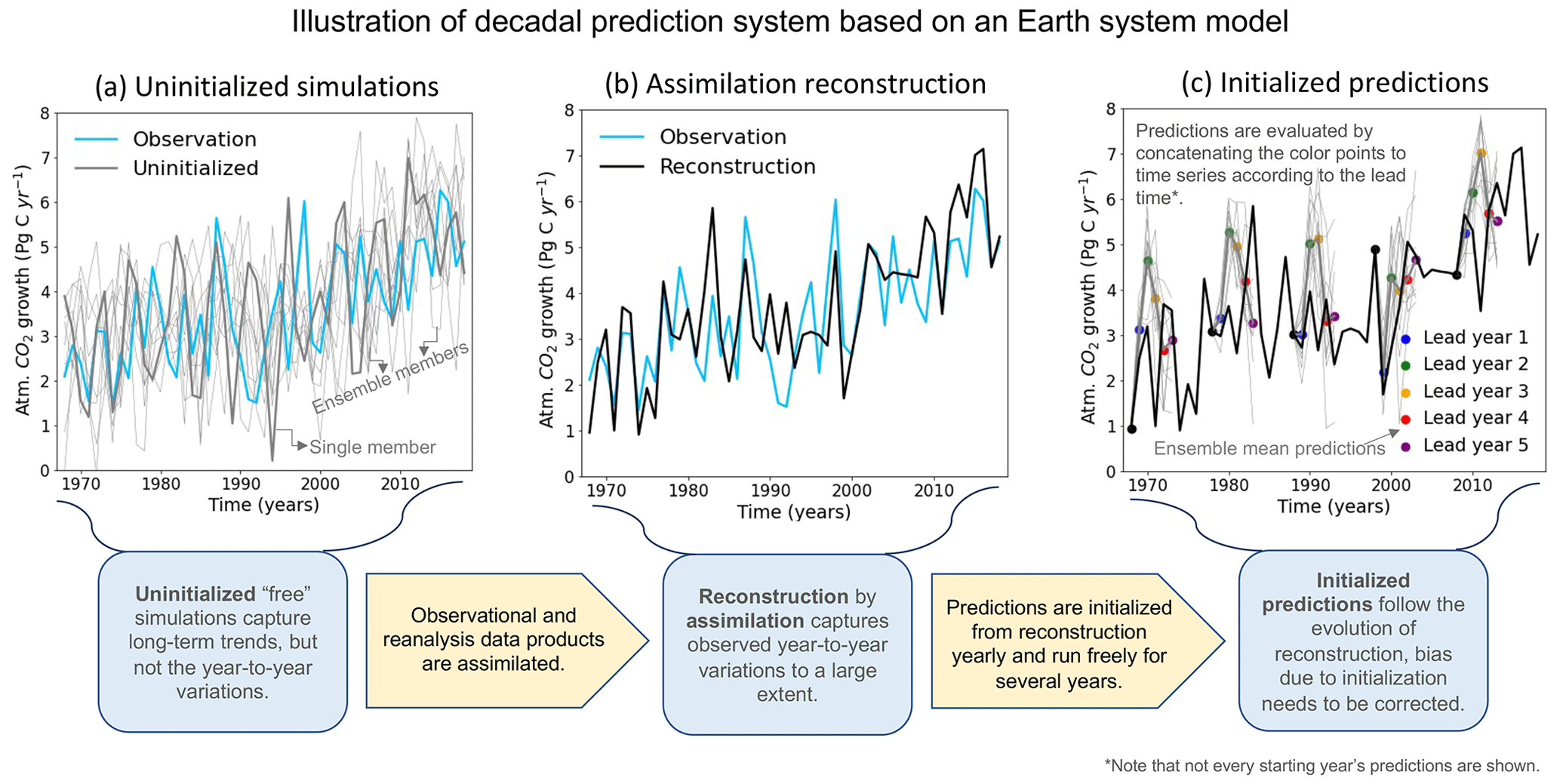
Figure 1 Illustration of the decadal prediction system based on the MPI Earth system model. The illustrated time series of the atmospheric CO₂ growth rate shows annual means from model simulations plotted together with observations from the Global Carbon Project (GCP). We conduct three sets of simulations (from left to right in sequential order): (a) uninitialized “free” simulations, which are the same as the freely evolving Coupled Model Intercomparison Project (CMIP) historical type simulations, (b) an assimilation simulation to reconstruct the evolution of the climate and carbon cycle towards the real world by nudging the model towards observation and reanalysis data during its integration, and (c) initialized predictions started from reconstruction states produced by the assimilation simulation and integrated freely (i.e., no nudging towards observations) for 5 years. The time series in (a) shows that the uninitialized simulations capture the long-term trend well, but the year-to-year variations are out of phase with the observations. The time series in (b) shows that the assimilation simulation forces the variations in the uninitialized freely run simulation towards the real world and results in a reconstruction that is closer to the observations. Panel (c) shows the reconstruction together with the 5-year-long initialized predictions (i.e., hindcasts). To make the illustration more clear, only predictions with starting years at 10-year intervals are shown.

2.2 Assimilation methods

Similar to our previous concentration-driven decadal prediction systems (Li et al., 2019), the assimilation is done by nudging the simulated ocean 3-D temperature and salinity anomalies towards the ECMWF ocean reanalysis system 4 (ORAS4) (Balmaseda et al., 2013). Additionally, we nudge the simulated values towards atmospheric 3-D full-field temperature, vorticity, divergence, and log of surface pressure from ECMWF Re-Analysis ERA40 (Uppala et al., 2005) during the period 1959–1979 and ERA-Interim (Dee et al., 2011) during the period 1980–2018. The sea ice concentration is nudged towards the National Snow and Ice Data Center (NSIDC) satellite observations (as described in Bunzel et al., 2016). The nudging is applied at every model time step but with a different relaxation time, i.e., a relatively longer relaxation time of 10 d is used for the ocean temperature and salinity, and shorter relaxation times of 6, 24, and 48 h are used for the atmospheric vorticity, temperature and pressure, and divergence, respectively. The chosen variables for assimilation and their respective relaxation time are selected based on previous investigations of decadal climate predictions based on the MPI-ESM (Marotzke et al., 2016). Direct assimilation of the carbon-cycle-related variables is not included because of the limited available data; instead, we found that the global carbon cycle is well captured by assimilating only physical variables (Li et al., 2016, 2019; Lovenduski et al., 2019b, a; Ilyina et al., 2021). Furthermore, a recent study based on a perfect-model framework (i.e., based on simulations in which the model tries to predict itself) revealed that direct assimilation of the global carbon cycle only brings trivial improvement to the predictive skill of the global carbon cycle (Spring et al., 2021). To avoid spurious upwelling in the equatorial region caused by assimilation (Park et al., 2018), we exclude the equatorial band of 5^∘ S–5^∘ N from being nudged towards observation-based ocean data.

2.3 Carbon budget decomposition with CBALONE simulations

The GCB from GCP is decomposed into five terms plus an imbalance term: the two emission terms from fossil fuel and land use changes and the three sink terms for the natural terrestrial sink, ocean sink, and atmospheric growth on annual timescales. The fossil fuel emissions are prescribed as forcing, and the terrestrial and ocean carbon sinks and atmospheric growth terms are simulated and can therefore be directly derived from the ESM. However, only the net land–atmosphere exchange is directly deducible from an ESM, which is the sum of land use change emissions and the natural terrestrial sink. In order to separate the two land-related fluxes, we use a standalone component of JSBACH called CBALONE as a diagnostic for a direct comparison with the land-use emissions term from the GCP (Friedlingstein et al., 2019). CBALONE is forced by the MPI-ESM daily outputs including 2 m air temperature, soil temperature, precipitation, net primary productivity (NPP) per plant functional type (PFT), leaf area index (also per PFT), and maximum wind. We run two parallel simulations, i.e., one with anthropogenic land use changes and another without those changes, differencing the two simulations results in the land-use-change-induced emissions from the land sink. More details on this method of separating the land-use-change-induced emissions can be found in Loughran et al. (2021).

2.4 Predictive skill quantification

The focus of this study is on global mean variations in atmospheric CO₂ and globally integrated air–sea and air–land CO₂ fluxes on annual timescales. The initialized simulations are investigated according to their lead time, i.e., for how many model years they have been freely integrated after restarting from the assimilation simulation. The time series of initialized simulations at a lead time of 1 year (2, 3, 4, and 5 years) combine the first year (second, third, fourth, and fifth year) predictions from initialized simulations of all the starting years from 1960–2018. Therefore, the time series at lead time of 1 year (2, 3, 4, and 5 years) corresponds to the period 1961–2019 (1962–2020, 1963–2021, 1964–2022, and 1965–2023). Illustration of how the time series are concatenated is shown in Fig. 1C. The analyses of predictive skill quantification are based on the combined time series. Bias correction is an unavoidable topic for decadal predictions due to an initial shock, which varies with lead time (Boer et al., 2016; Meehl et al., 2021). The decadal prediction studies mostly present anomalies with a focus on variations by removing the climatological mean and/or trend bias due to model drift caused by the initialization of the model based on observations. The anomalies are calculated relative to the respective climatology according to the lead time (Boer et al., 2016; Meehl et al., 2021). To infer predictions of absolute values of the atmospheric CO₂ concentration, the respective anomalies from the predictions are added to the best estimates of climatology and trend from data; here the atmospheric CO₂ observations from NOAA_GML (Dlugokencky and Tans, 2020) are used.

The predictive skill is quantified by the anomaly correlation coefficient, and the anomalies are calculated by removing the respective climatological mean state. In that sense, the climatological mean bias is removed and the coherence reflects the multi-year variations for which we evaluate the predictions. Here the climatological mean state is based on the ensemble mean of the focus time period: 1970–2018 for Figs. 1–6 and the last 10 years for Figs. 7–8. We exclude the first 12 years, i.e., 1958–1969, from the analyses and focus on the period from 1970–2018 because the assimilation in the first decade is affected by model adjustment. As an example, the spatial pattern of climatological mean ocean net primary production and phosphate nutrient concentration are shown in Fig. A2 in comparison with the respective observations. For the atmospheric CO₂ concentration, which has high correlations close to 1 with observations because of the coherent linear trends, we have also added the root-mean-square error (RMSE) metric to investigate the added value of assimilation and initialization. In this study, the significance of the predictive skill is tested with a nonparametric bootstrap approach (Goddard et al., 2013). The analyses are based on annual mean data with a focus on the frequency of interannual to multi-year variations.

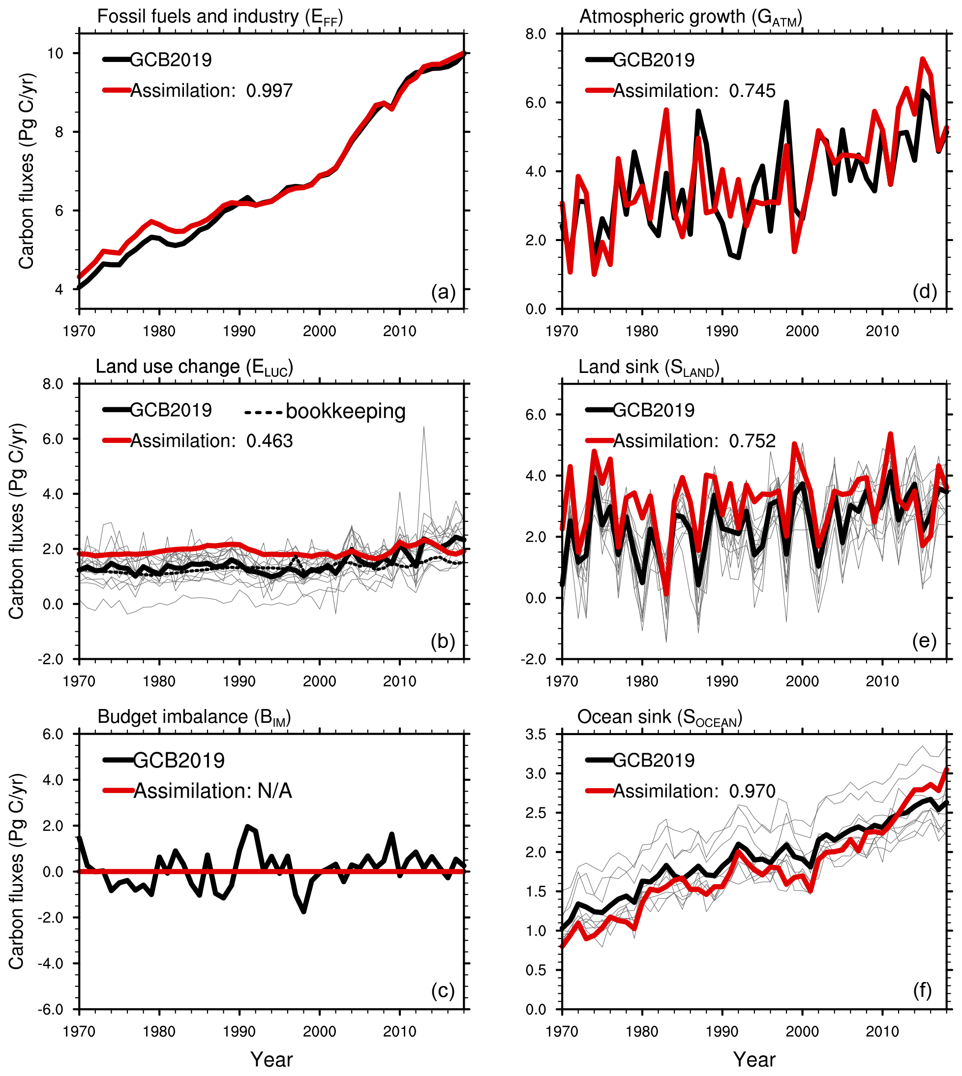
Figure 2 Time series of (a) fossil fuel and industry CO₂ emissions (E_FF), (b) emissions from land use change (E_LUC), (c) the budget imbalance (B_IM) that is not accounted for by the other terms, (d) atmospheric carbon growth rate (G_ATM), (e) the natural terrestrial carbon fluxes (S_LAND), and (f) air–sea CO₂ fluxes (S_OCEAN) from MPI-ESM1.2-LR assimilation in comparison to the Global Carbon Budget (GCB 2019, Friedlingstein et al., 2019). Emissions (a, b) are positive into the atmosphere, while sinks (d, e, f) are positive into their respective compartments. A positive B_IM means a higher sum of emissions than sinks. The thin grey curves in (b), (e), and (f) show individual GCB standalone model results. The numbers in the legend show the correlation coefficients between carbon fluxes from the assimilation simulation and GCB2019.

3 Reconstruction of the global carbon budget

By incorporating observation-based information, the assimilation simulation from the decadal prediction system based on the MPI-ESM captures the evolution of the GCB as well as the climate in observations. The time series of carbon fluxes from the MPI-ESM assimilation simulation in comparison to the data and suite of simulations from GCB2019 are shown in Fig. 2.

The CO₂ emissions from fossil fuels and industry are generally consistent with those from GCB2019 but with a slight difference in the 1960–1990s since the assimilation simulation uses the CO₂ emission forcing provided by CMIP6 for historical and SSP2-4.5 simulations. This highlights the uncertainty in the CO₂ forcing, which affects the change in the simulated atmospheric CO₂ concentration as it is a cumulative quantity. The CMIP6 CO₂ emission forcing yields 8.20 PgC higher cumulative emissions than those from the GCB2019, which is equivalent to a difference of atmospheric CO₂ of about 1.93 ppm assuming that 50 % of the emissions stay in the atmosphere (i.e., by dividing 4.10 PgC with a factor of 2.124 PgC ppm⁻¹, Ballantyne et al., 2012). This discrepancy in CO₂ emissions might explain to some extent why the simulated atmospheric CO₂ concentration is a few parts per million higher than the NOAA_GML observations (Dlugokencky and Tans, 2020) (Fig. A3). However, this small difference of a few parts per million in atmospheric CO₂ concentration magnitude does not noticeably affect the interannual variations in CO₂ fluxes and the corresponding atmospheric carbon increment (see Fig. 2d–f).

The land-use-change-induced emissions diagnosed by CBALONE are within the range of GCB2019 multi-model (including JSBACH) simulations from Dynamic Global Vegetation Models (DGVMs) (Fig. 2b). The estimates from bookkeeping models show smaller variations than those produced by the DGVMs. Note that the GCP uses the bookkeeping approach for the land-use emissions term. The term bookkeeping implies that carbon fluxes are determined from area changes in vegetation types with different vegetation and soil carbon densities, and specific response curves characterizing the evolution of decay of deforested biomass and recovery of natural vegetation thereafter. Biomass and soil carbon densities may be based on recent observations or models but are generally kept fixed in time, i.e. the effect of changes in environmental conditions are not accounted for. The DGVMs by contrast (which are used to provide only an uncertainty range around the bookkeeping models in the GCBs from the GCP) calculate land use emissions under transient environmental conditions. This implies first that interannual variability in bookkeeping models is only driven by land use change but not by climate variability, which makes the DGVM estimates of land use change (LUC) emissions in general more variable from year to year than the bookkeeping estimates. Second, the DGVM-based land-use emissions estimates include the so-called “loss of additional sink capacity” (Pongratz et al., 2014), which refers to the carbon that could have been stored in forests additionally over the course of history (e.g., due to the “CO₂ fertilization” effect) had these forests not been cleared by the expansion of agriculture and forestry. This loss of additional sink capacity generally increases over time and amounts to about 40 % (0.8 ± 0.3 PgC yr⁻1) of the emissions calculated by the DGVMs over 2009–2018 (Obermeier et al., 2021). This explains why DGVM estimates in Fig. 2b show higher emissions than bookkeeping estimates in recent decades. The DGVM- and expert-based uncertainty range around the GCP bookkeeping estimates for LUC emissions is large and MPI-ESM-based land use change emission estimates have been found to be at the high end of the GCP estimates for all decades by Loughran et al. (2021), consistent with our findings.

The annual assessment from GCP has a budget imbalance term. This is because the individual budget terms are based on separate measurements, together with ocean and land model simulations, which are not linked to each other in an internally consistent manner (Friedlingstein et al., 2019). In this study, we assimilate atmosphere and ocean data products within a fully coupled ESM that considers their interactions. The assimilation ensures the evolution of the carbon cycle and climate towards the real world, and in contrast to the GCP, the budget is closed within the Earth system, i.e., no budget imbalance occurs by design (Fig. 2c). Therefore, the assimilation simulation based on a fully coupled ESM enables better attribution of the GCB variations than when an imbalance is present. The current method used by the GCP (Friedlingstein et al., 2019) is based on the directly measured atmospheric CO₂ increment and has the advantage of representing the actual evolution of atmospheric CO₂. Our ESM-based assimilation shows a high correlation of 0.75 with the atmospheric CO₂ measurements but still needs to be improved. Further efforts are required to constrain the atmospheric CO₂ from observations.

Atmospheric carbon growth rate and carbon fluxes are reasonably well reproduced in emission-driven assimilation with prognostic atmospheric CO₂ (Fig. 2d–f). The atmospheric carbon growth and the land carbon sink show more pronounced variations on interannual timescales; however, the ocean carbon sink has more pronounced variations on decadal timescales. These variations are captured in the assimilation, with high correlations between the results from the assimilation simulation and the GCB2019 of 0.75, 0.75, and 0.97 for the atmospheric growth, air–land CO₂ fluxes, and air–sea CO₂ fluxes, respectively.

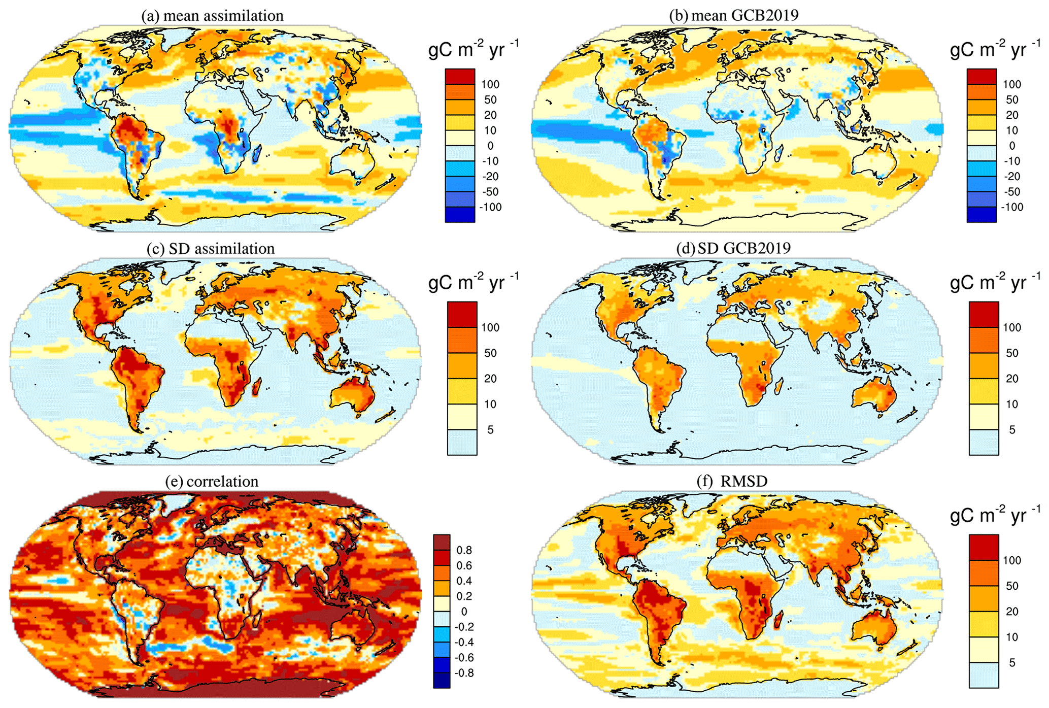
Figure 3 Spatial distribution of the CO₂ fluxes from model assimilations compared to GCB2019. Climatological mean CO₂ fluxes into the land and ocean from the atmosphere in assimilation (a) and Global Carbon Budget (GCB 2019, Friedlingstein et al., 2019) estimates (b). Temporal variability, i.e., standard deviation, of CO₂ fluxes in the assimilation simulation (c) and GCB2019 (d). Correlation and root-mean-square deviation (RMSD) between assimilation and GCB2019 are shown in (e) and (f), respectively. The results are based on annual mean data for the time period 1970–2018. Positive values in (a) and (b) refer to CO₂ fluxes into the ocean or land.

The spatial distribution of climatological mean CO₂ fluxes, their variability expressed as standard deviation, and the comparison in carbon fluxes between GCB2019 and the MPI-ESM assimilation are shown in Fig. 3. The mean states show a CO₂ influx into the ocean and land in the mid- to high-latitudes, and outgassing into the atmosphere in tropical areas, especially over the tropical Pacific (Fig. 3a–b). The variability of CO₂ over land is larger than that over the ocean; and the magnitude of variability is larger in the assimilation simulation than in the GCB2019 (Fig. 3c–d). This is expected as the GCB2019 is a multi-model mean estimate and therefore smooths out part of the high-frequency variability. The correlation of CO₂ fluxes between the assimilation simulation and GCB2019 is high over the ocean, while the correlation is relatively low over the land (Fig. 3e). The root-mean-square deviation (RMSD) scales with the magnitude of carbon fluxes, i.e., with larger values on land than over ocean (Fig. 3f). The large RMSD, especially over land, is because of the relatively low coherence of CO₂ fluxes and the larger values of CO₂ fluxes in the MPI-ESM single model simulation than in a smoothed magnitude of fluxes in GCB2019 from the multi-model mean simulations. The difference in the magnitude of fluxes between assimilation and GCB2019 data is more prominent in local areas (Fig. 3a–d) than in the global average (Fig. 2e).

In general, the historical GCB is well reproduced by the MPI-ESM when assimilating observational products, which enables a quantification of the GCB within a closed Earth system, showing that prediction systems yield internally consistent estimates of the air–sea and air–land CO₂ fluxes and are able to provide complementary information, in addition to the estimates provided by the GCP, for evaluating annual GCB.

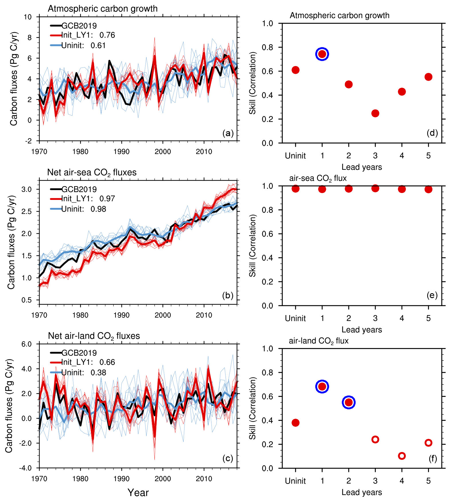
Figure 4 Time series of atmospheric carbon growth rate, i.e., G_ATM (a), net air–sea CO₂ fluxes, i.e., S_OCEAN (b), and net air–land CO₂ fluxes, i.e., E_LUC+S_LAND (c), from the initialized simulations at a lead time of 1 year together with values from the uninitialized simulations and estimates from the 2019 Global Carbon Budget (GCB 2019, Friedlingstein et al., 2019). Positive values in (b) and (c) indicate CO₂ fluxes into the ocean or land. The numbers in the legend show the correlation coefficients between the simulations and GCB2019, and the ensemble mean data are used for this correlation calculation. Predictive skill of the atmospheric carbon growth rate, i.e., G_ATM (d), air–sea CO₂ fluxes, i.e., S_OCEAN (e), and net air–land CO₂ fluxes, i.e., E_LUC+S_LAND (f), in reference to the Global Carbon Budget (GCB 2019, Friedlingstein et al., 2019). The filled red circles on top of the open red circles show that the predictive skill is significant at a 95 % confidence level, and the additional larger blue circles indicate an improved significant predictive skill due to initialization in comparison to the uninitialized simulations. We use a nonparametric bootstrap approach (Goddard et al., 2013) to assess the significance of predictive skill. The results are based on annual mean data for the time period of 1970–2018.

Figure 5 The same as Fig. 4 but with linearly detrended time series.

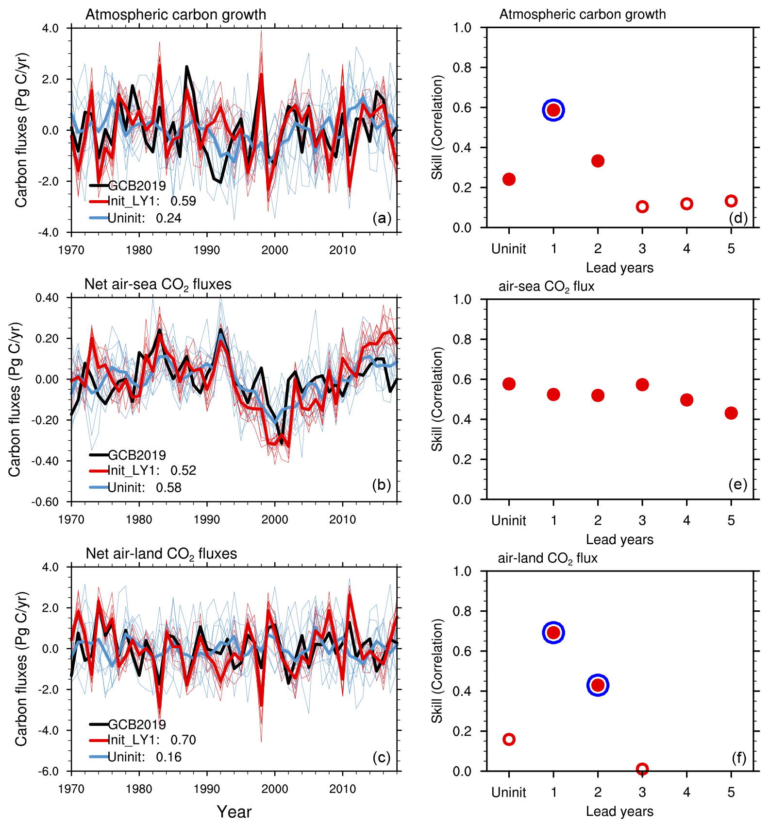
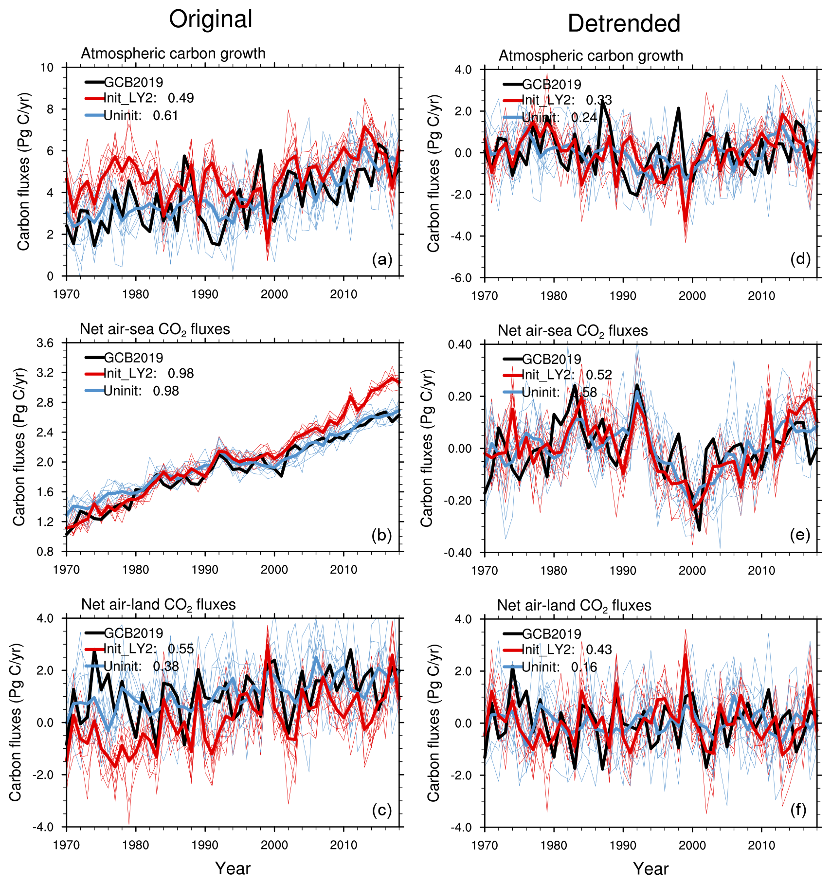
Figure 6 Time series at a lead time of 2 years for atmospheric carbon growth rate, i.e., G_ATM (a), net air–sea CO₂ fluxes, i.e., S_OCEAN (b), and net air–land CO₂ fluxes, i.e., E_LUC+S_LAND (c), from the initialized simulations together with values from the uninitialized simulations and estimates from the 2019 Global Carbon Budget (GCB 2019, Friedlingstein et al., 2019). Panels (d), (e), and (f) are the same as (a), (b), and (c) but show the linearly detrended time series. The time series shown are based on annual mean data for the time period of 1970–2018. Positive values in panels (b), (c), (e), and (f) imply CO₂ fluxes into the ocean or land. The numbers in the legend show the correlation coefficients between the simulations and GCB2019, and the ensemble mean data are used for the calculation.

4 Predictability of the global carbon budget

The initialized predictions start from assimilation states which are close to observations. Therefore, information from the observations is incorporated into the prediction system through realistic initial states of the components of the climate system, which enables a more realistic evolution of the global carbon cycle and climate that follows the trajectory of observations until the predictability horizon is reached.

To support the GCP in predicting the next year's GCB one year in advance, we also investigate the predictability, focusing on model hindcasts at a lead time of 1 year. As shown in Figs. 4 and 5, the initialized simulations at a lead time of 1 year show high correlations with GCB2019. The correlations of global atmospheric CO₂ growth, net air–sea CO₂ fluxes and net air–land CO₂ fluxes are 0.59, 0.52, 0.70 after removing the linear trends (Fig. 5a, c, e); the correlation of the original time series are 0.76, 0.97, and 0.66 (Fig. 4a, c, e). The initialized simulations at a lead time of 2 years still resemble the variations in the GCB2019, with correlations of 0.49 and higher (Fig. 6a, c, e), and the detrended time series also show higher correlations than the detrended uninitialized simulations (Fig. 6b, d, f). This suggests that internal variability can be constrained by initialization. As for atmospheric carbon growth, the initialized simulations at a lead time of 2 years show coherent interannual variations compared to GCB2019, albeit with a smaller correlation (0.49) than that of the historical freely evolving run (0.61), primarily due to the trends in atmospheric CO₂ growth rate in the freely evolving run and in GCB2019. After detrending, the correlations are higher in the initialized simulations than in the uninitialized simulations (comparing Fig. 6a, d).

The initialized and uninitialized simulations show a comparably good match to GCB2019 with respect to the net CO₂ flux into the ocean (with a high correlation up to 0.98) (Fig. 4b). The variations in the globally integrated ocean carbon sink are driven primarily by external forcing rather than internal variability, as found in McKinley et al. (2020). Figures 4b and 5b show that the ocean carbon sink variations (especially on decadal timescales) in the historical freely evolving uninitialized run are simulated reasonably well.

The net carbon flux into land shows higher correlations for initialized simulations at lead time of 1 year and 2 years than those for uninitialized simulations (Figs. 4c, 5c and 6c, f). This indicates that the interannual variations are better captured in the initialized model system even after 2 years of free integration. This result implies a predictability of the air–land CO₂ flux for up to 2 years. The air–land CO₂ fluxes are regulated by El Niño–Southern Oscillation (ENSO) variations (Loughran et al., 2021; Dunkl et al., 2021), and the poor skill in predicting ENSO limits the predictability of the air–land CO₂ fluxes. However, the predictive skill of air–land CO₂ of 2 years is beyond the predictability horizon of ENSO, which is limited to a seasonal scale.

We further quantify the predictive skill of the GCB through all the lead times up to 5 years (Fig. 4b, d, f and Fig. 5b, d, f). The correlation skill relative to GCB2019 is significant for the lead time of 5 years in the atmospheric carbon growth and the ocean carbon sink. However, the skill for the air–land CO₂ flux is not statistically significant at the 95 % level after lead time of 2 years (Fig. 4d–f). The improved predictive skill of initialized hindcasts compared to the historical uninitialized run occurs at a lead time of 1 year for atmospheric carbon growth and at a lead time of 2 years for air–land CO₂ flux. The detrended results (Fig. 5d–f) are similar to those from the original time series. The correlation of atmospheric carbon growth at a lead time of 2 years in the initialized hindcasts, compared to the estimates from the GCB2019, is higher than the uninitialized historical run when detrended. This indicates the contribution of a linear trend to the skill of atmospheric carbon growth in uninitialized historical runs as shown in Fig. 4d. Although the improvement in predictive skill in the initialized simulation relative to the uninitialized simulation is not significant for atmospheric CO₂ growth rate, the correlations of both initialized simulations at a lead time of 2 years and the uninitialized simulations are significantly high, as indicated with solid red dots. This suggests the predictability of atmospheric carbon growth for up to 2 years.

From our MPI-ESM1.2-LR initialized hindcasts, we find that predictive skill of the air–sea CO₂ flux is relatively high for up to 5 years and that of the air–land CO₂ fluxes is up to 2 years. This is consistent with previous studies without an interactive carbon cycle (Ilyina et al., 2021; Lovenduski et al., 2019a, b). Here we have extended the prediction system for emission-driven simulations, enabling prognostic CO₂ and preserving features of predictability. The prognostic CO₂ from the novel emission-driven decadal prediction system suggests a predictive skill of 2 years for the atmospheric CO₂ growth rate.

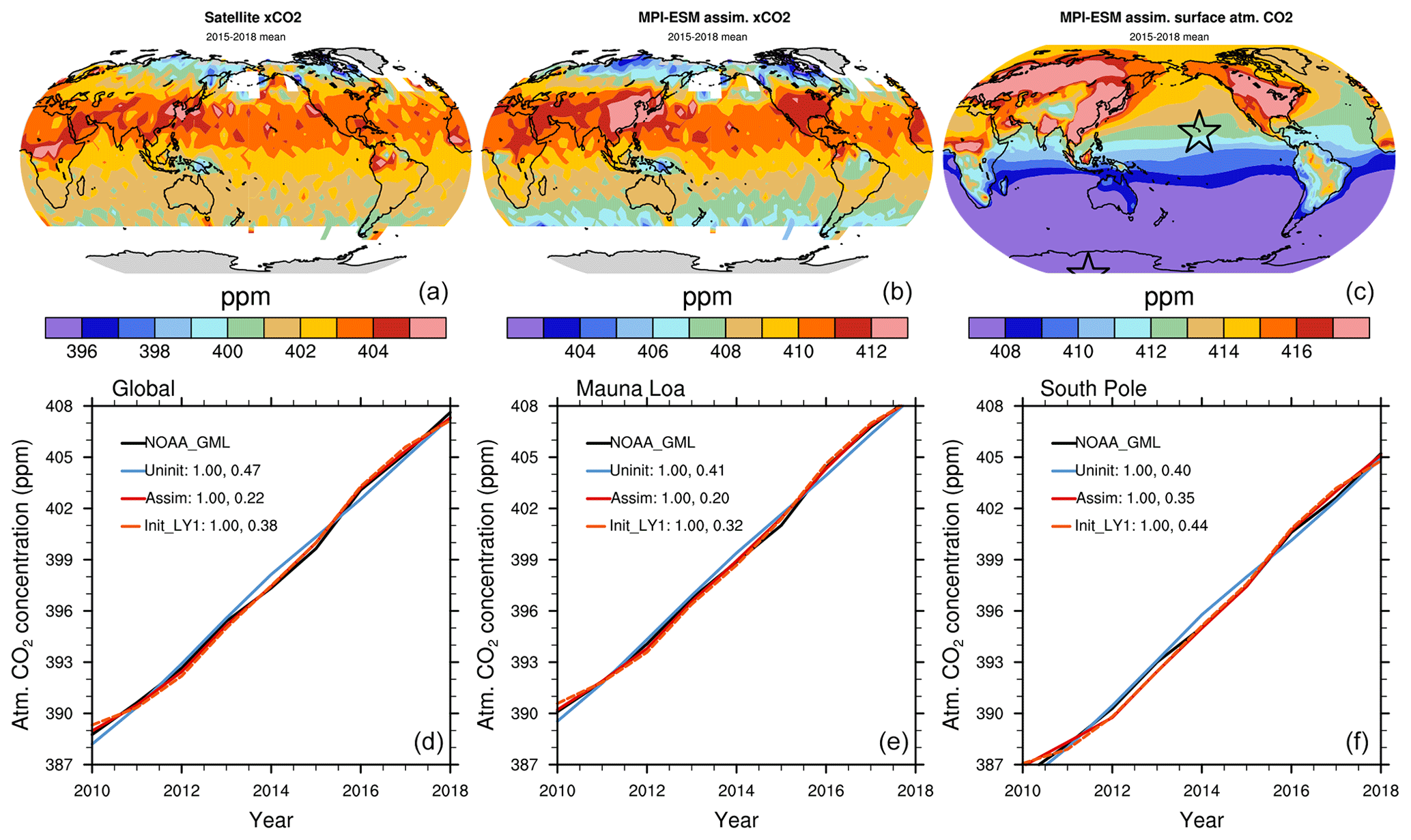
Figure 7 Spatial distribution of 2015–2018 mean satellite-based Obs4MIPs XCO₂ (a), model assimilation of XCO₂ (resampled according to satellite data availability) (b), and model assimilation of atmospheric CO₂ concentration at 1000 hPa level (c). A short time period of 2015–2018 is used because of the limited temporal coverage of satellite data. The satellite XCO₂ data product is obtained from the Climate Data Store Copernicus Climate Change Service (Reuter et al., 2013). The conversion of model-simulated CO₂ to XCO₂ is performed according to Gier et al. (2020) (their Appendix A). Atmospheric CO₂ concentration as a global average (d), at Mauna Loa (e), and at the South Pole (f) from the uninitialized (Uninit) and assimilation (Assim) simulations and initialized simulations at a lead time of 1 year (Init_LY1) compared to observations over the 2010–2018 period. The locations of Mauna Loa and the South Pole are shown in (c). The numbers in the legend show the correlation (left) and root-mean-square error (RMSE, right) of the simulations relative to observational data from NOAA_GML (Dlugokencky and Tans, 2020). The simulated time series from the MPI-ESM simulations, including uninitialized, assimilation, and initialized simulations, are bias corrected by removing the difference in mean states and the linear trend between observations and simulations according to Boer et al. (2016).

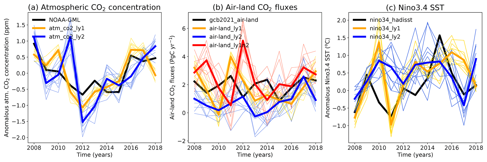
Figure 8 (a) Time series of atmospheric CO₂ concentration anomalies from initialized simulations at a lead time of 1 year and 2 years compared to the NOAA_GML observations (Dlugokencky and Tans, 2020) over the last 10 years. Anomalies are calculated by detrending the time series and with the climatological mean removed. (b) Time series of CO₂ fluxes from initialized simulations at a lead time of 1 year and 2 years together with estimates from the GCB2019. The red curves present the sum of predictions at a lead time of 2 years and the previous year of prediction at a lead time of 1 year (air–land_ly1n2). (c) Time series of nino3.4 SST from model simulations and HadISST (Rayner et al., 2002). The time series are original model outputs and concatenated according to the lead time of years.

5 Atmospheric CO₂ concentration

Figure 7 shows the spatial pattern and time series of atmospheric CO₂ concentration from MPI-ESM simulations, including uninitialized, assimilation, and initialized simulations, together with the satellite XCO₂ (i.e., atmospheric column-average dry-air mole fraction CO₂) and NOAA_GML observations for the period 2015–2018. The XCO₂ from the assimilation simulation (Fig. 7b) shows the spatial distribution of atmospheric CO₂ concentration, which compares well with the satellite XCO₂ (Fig. 7a). High CO₂ concentrations are found in the tropics to midlatitudes of the Northern Hemisphere. Relatively low CO₂ concentrations are found in the Southern Hemisphere and the polar regions. Note the model simulation is several parts per million higher than the satellite data, and this deviation can be attributed back to the uninitialized historical simulation (see Fig. A3). Additionally, the satellite data do not cover all the seasons in high latitudes, and therefore the sampled values from the assimilation simulation also better represent the summer season's XCO₂ in those regions. The surface level CO₂ shows a more dominant higher concentration in the Northern Hemisphere than in the Southern Hemisphere (Fig. 7c). Here we also compare the surface atmospheric CO₂ concentration with the measurements at the Mauna Loa and South Pole stations (locations are shown as stars in Fig. 7c).

The atmospheric carbon burden and therefore CO₂ concentration is an accumulative quantity and mainly shows a linear increasing trend in recent decades in response to increasing anthropogenic emissions. Systematically lower or higher simulated carbon uptake by land and ocean compared to the real world therefore accumulates over the time period while the model is integrated. The simulated atmospheric CO₂ concentration can deviate relative to observations. In the MPI-ESM, simulated global mean atmospheric CO₂ concentration is around 8 ppm higher compared to the observations in the 2010s (see Fig. A4). The NOAA_GML data represent the average of atmospheric CO₂ over marine surface sites (Dlugokencky and Tans, 2020), and these values are slightly lower than the values over land since the anthropogenic CO₂ emissions occur mainly on land. The time series shown in Fig. 7d–f are bias corrected by removing the difference of mean states and linear trends between observations and simulations according to Boer et al. (2016).

The atmospheric CO₂ concentration from assimilation shown follows the evolution of NOAA_GML observations well, with a RMSE of 0.22 ppm, which is better than the uninitialized historical run with a RMSE of 0.47 ppm (Fig. 7d). In general, the RMSE increases from a lead time of 1 year to 2 years and decreases until a lead time of 5 years at both the global and observatory sites of Mauna Loa and the South Pole (Figs. A5 and A6). The relatively low predictive skill at a lead time of 2 years in atmospheric CO₂ concentration is because the model failed to predict the neutral ENSO events in 2010 and La Niña in 2011 and instead predicts a strong El Niño in both years (Fig. 8c). The corresponding air–land CO₂ fluxes are reversed, i.e., the land takes up less CO₂ than expected in 2011 (Fig. 8b solid blue curve and solid black curve). As the atmospheric CO₂ concentration is a cumulative quantity, the magnitude of atmospheric CO₂ concentration is affected by the CO₂ fluxes in the current and previous years. We also present the cumulative air–land CO₂ fluxes of the first- and second-year prediction (see the red curves in Fig. 8b), and the variations in cumulative air–land CO₂ fluxes are reversed compared to those in atmospheric CO₂ concentration changes at a lead time of 2 years, as shown in Fig. 8a (blue curves). The results indicate that the air–land CO₂ flux and corresponding atmospheric CO₂ has predictive skill, though the skill at a lead time of 2 years is degraded by the poor predictive skill of ENSO in some starting year predictions.

This retrospective prediction demonstrates the ability of an ESM-based decadal prediction system in reconstructing and predicting the global carbon cycle via only assimilating the physical atmosphere and ocean fields. As presented in Fig. 5b, d, and f, the hindcasts also show a predictive skill of 5 years for air–sea CO₂ fluxes and 2 years for air–land CO₂ fluxes and atmospheric carbon growth. Hence, the ability of ESMs to predict the next year's GCB is high.

6 Conclusions

For the first time, we have extended a decadal prediction system based on the MPI-ESM to include an interactive carbon cycle driven by fossil fuel emissions that enables prognostic atmospheric CO₂ predictions. The new assimilation and initialized predictions have one more degree of freedom, i.e., prognostic atmospheric CO₂, and this framework represents the global carbon cycle as it operates in the real world.

The variations in atmospheric carbon growth rate and CO₂ fluxes among the atmosphere, ocean, and land are well reconstructed in our assimilation simulations, with high correlations (0.75, 0.97, and 0.75) compared to the estimates from the GCB2019. This provides confidence in the quantification of the GCB in a closed system within an Earth system model. Reconstructions of the GCB based on ESMs are therefore able to potentially provide additional lines of evidence for quantifying the annual GCB and open new opportunities in assessing the efficiency of carbon sinks. In particular, this approach eliminates the budget imbalance term that arises in GCBs of the GCP due to the combination of various and not fully consistent model and data approaches.

To further support the GCP in predicting next year's GCB, the focus of the predictability investigations is on the lead time of 1 year. The results show high confidence in predicting the GCB for the next year with the MPI-ESM prediction system. We further demonstrate that retrospective predictions of the GCB have a predictive skill for up to 5 years for air–sea CO₂ fluxes and up to 2 years for air–land fluxes and atmospheric carbon growth rate. This indicates that the variations in atmospheric CO₂ are better reproduced in the assimilation and retrospective predictions than in the uninitialized freely evolving historical simulations.

The MPI-ESM decadal prediction framework preserves the high predictive power in an emission-driven configuration, simulating the atmospheric CO₂ growth rate with reasonable accuracy. In addition, the emission-driven decadal prediction system delivers the huge advantage of simulating the air–land and air–sea CO₂ fluxes in response to fossil fuel and land use change emissions, including all feedbacks in a consistent framework. Further future efforts that assimilate more observations to initialize ESMs and assess their predictive skill will lead to more reliable reconstructions and predictions of global estimates and spatial distributions of CO₂ fluxes and atmospheric CO₂. This study is based on simulations from a single ESM. Multi-model simulations that adopt a framework similar to that used in this study will allow for the identification of robust changes in the global carbon cycle expected to occur over the next few years.

We have demonstrated that the MPI-ESM-based emission-driven decadal prediction system exhibits the capability to reconstruct and predict the GCB and atmospheric CO₂ concentration variations. Such ESM-based applications will be a useful tool in supporting global carbon stocktaking in compliance with the goals of the Paris Agreement.

Appendix A

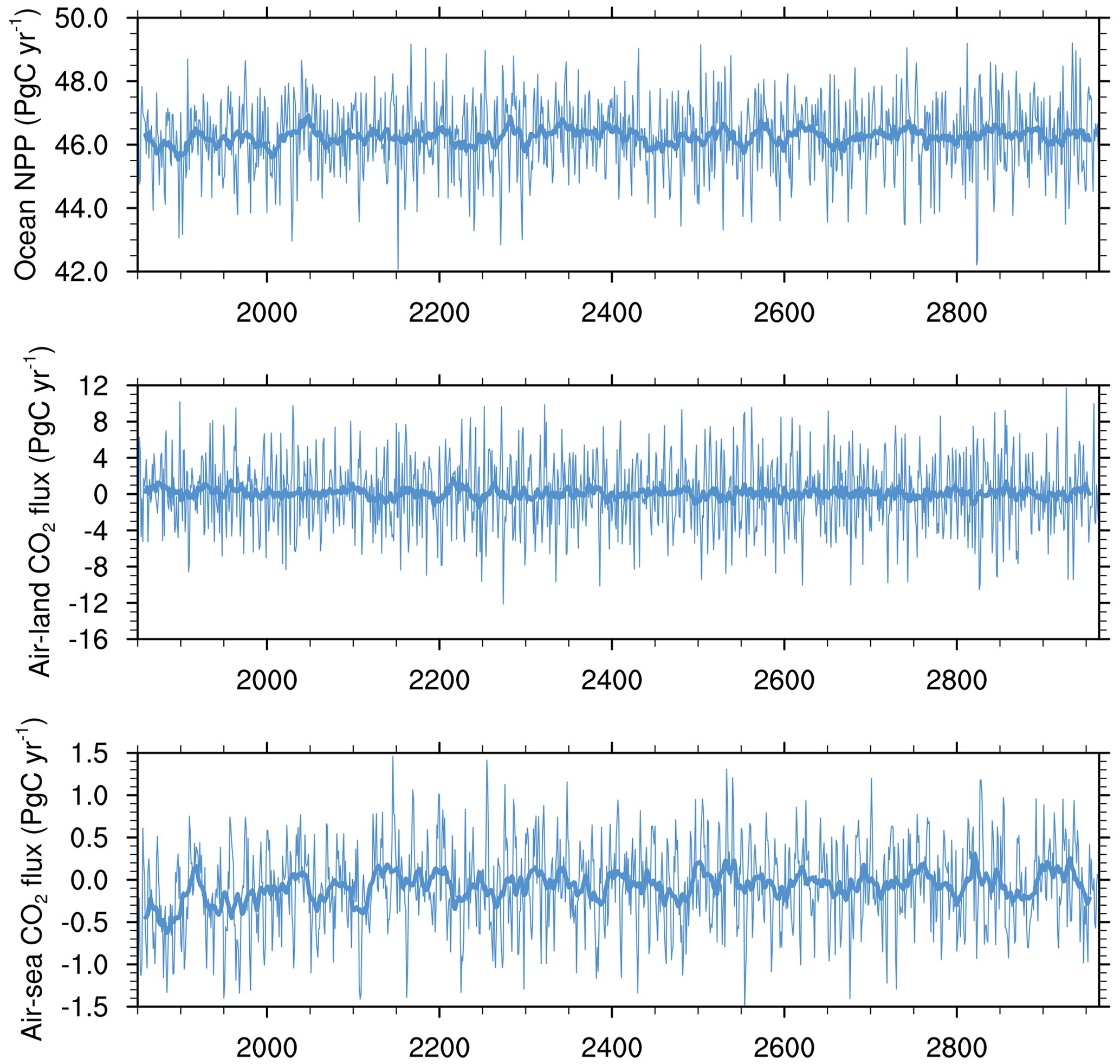
Figure A1 Time series of model simulations of ocean net primary production, air–sea CO₂ flux, and air–land CO₂ flux in the pre-industrial control run. The thin lines are annual mean time series, and the thick lines are their 20-year running means.

Figure A2 Climatological mean of ocean net primary production (NPP, a–c) and phosphate concentration (d–f) from observations and from model simulations. Observation-based NPP data are estimated from ocean color measurements obtained by the Sea-viewing Wide Field-of-view Sensor (SeaWiFS) instrument of the OrbView-2 satellite for the September 1997–December 2002 period and the Moderate Resolution Imaging Spectroradiometer (MODIS) of the Aqua satellite for the 2003–2014 period (Behrenfeld and Falkowski, 1997, http://science.oregonstate.edu/ocean.productivity/index.php, last access: 12 November 2019). Phosphate observations are from the World Ocean Atlas 2018 (Garcia et al., 2019). The corresponding NPP data from model simulations are averaged over the 1998–2017 period, and phosphate data are averaged over the 1970–2018 period according to the availability of the observation data.

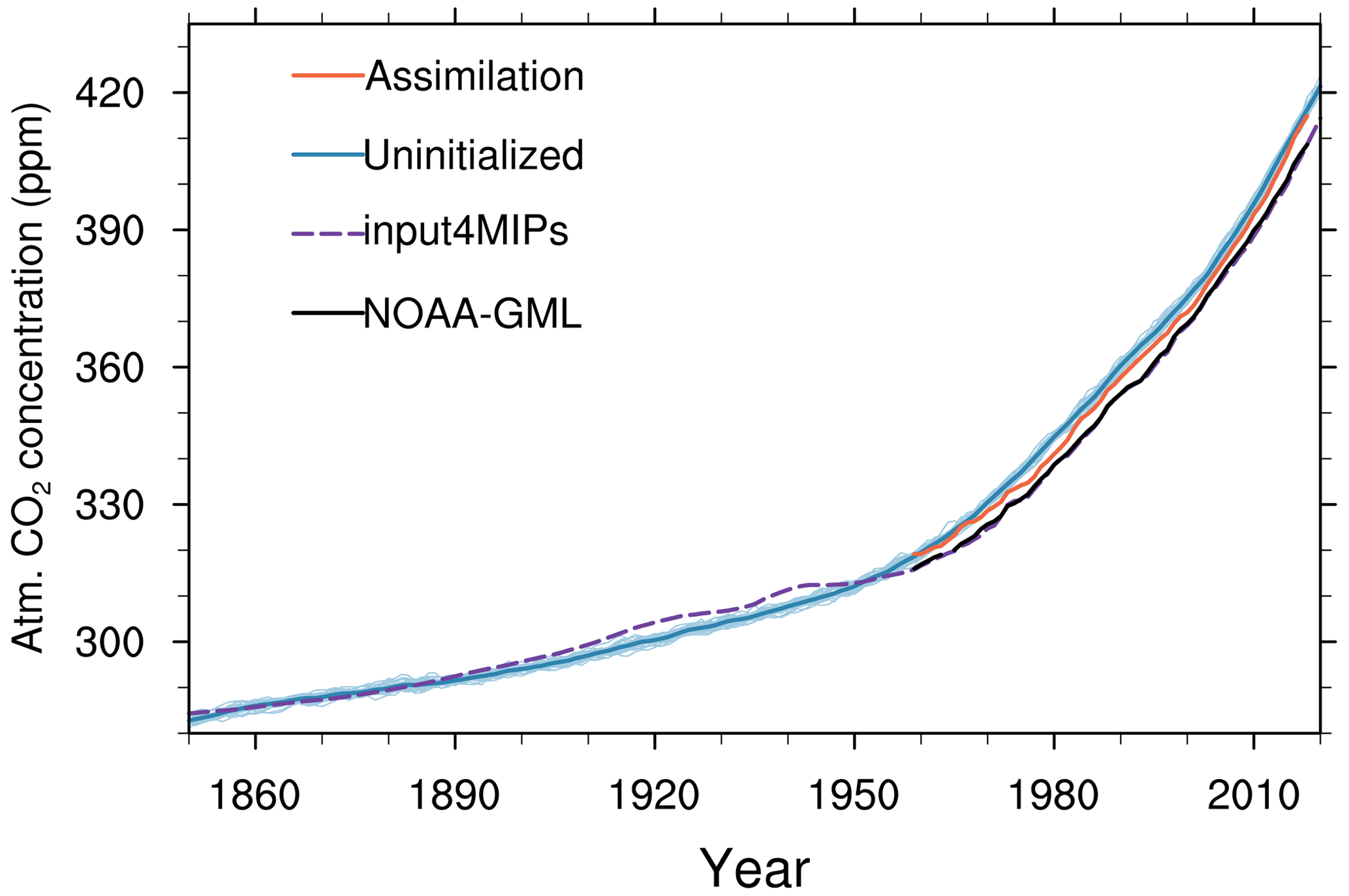
Figure A3 Time series of atmospheric CO₂ concentration from model simulations and observations from 1850 to 2020. The assimilation and uninitialized simulations are shown with solid orange and blue lines, respectively. The CMIP6 input4MIPs atmospheric CO₂ concentration forcing and the NOAA_GML observation (Dlugokencky and Tans, 2020) are shown with dashed blue lines and solid black lines, respectively.

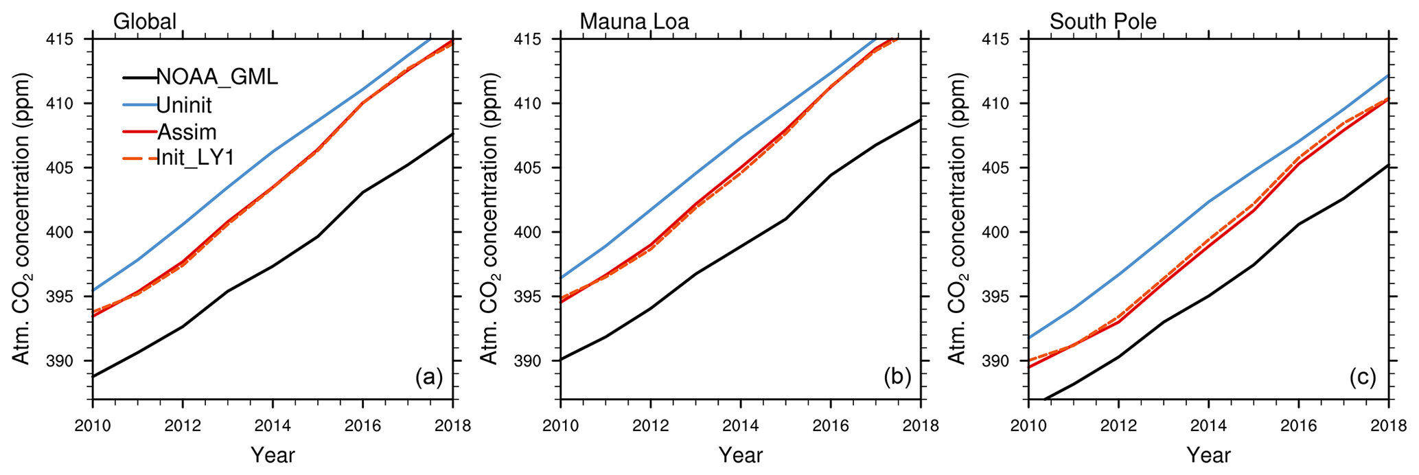
Figure A4 Atmospheric CO₂ concentration from the assimilation and initialized simulations at a lead time of 1 year together with NOAA_GML observations (Dlugokencky and Tans, 2020) over the last 10 years. The time series are original model outputs and concatenated according to the lead time of years.

Figure A5 Atmospheric CO₂ concentration from initialized simulations at a lead time of 2–5 years together with NOAA_GML observations (Dlugokencky and Tans, 2020) over the last 10 years. The time series are original model outputs and concatenated according to the lead time of years.

Figure A6 The same as Fig. A5 but with bias-corrected mean states and linear trends.

Table A1 Simulations based on MPI-ESM1.2-LR. The resolution for the atmosphere is T63L47 and for the ocean is GR15L40. The design of the prediction simulations is according to previous studies (Marotzke et al., 2016; Li et al., 2019). The assimilation starts from the end of the year 1958 in an uninitialized simulation. The nudging is strong; therefore, assimilation starting from a different uninitialized simulation would end up with similar evolution of the climate and carbon cycle. Figure 1 illustrates the simulations with evolution of atmospheric CO₂ growth rate together with observations. The initialized simulations start from the assimilation yearly from October 31st and run freely for 2 months plus 5 years afterwards. We have 59 runs for each ensemble of initialized simulations starting from 1960 to 2018 annually, and these run for 5 years and 2 months each, i.e., November 1960–December 1965 for starting year 1960, November 1961–December 1966 for starting year 1961, and so forth until November 2018–December 2023. The ensembles are generated with lagged 1 d initialization, i.e., the simulations start from 10 consecutive days from 31 October to 9 November. The ensembles for uninitialized simulations (shown as in Fig. A3) are generated by starting from different years of the control simulation (Fig. A1).

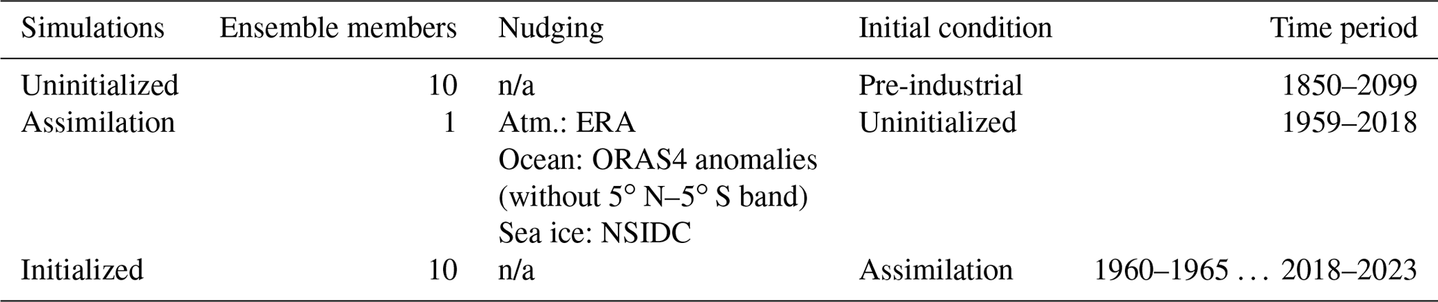
n/a: not applicable.