the Creative Commons Attribution 4.0 License.
the Creative Commons Attribution 4.0 License.
 | 28 Jul 2021
Abrupt climate change as a rate-dependent cascading tipping point
Johannes Lohmann
Daniele Castellana
Peter D. Ditlevsen
Henk A. Dijkstra
We propose a conceptual model comprising a cascade of tipping points as a mechanism for past abrupt climate changes. In the model, changes in a control parameter, which could for instance be related to changes in the atmospheric circulation, induce sequential tipping of sea ice cover and the ocean's meridional overturning circulation. The ocean component, represented by the well-known Stommel box model, is shown to display so-called rate-induced tipping. Here, an abrupt resurgence of the overturning circulation is induced before a bifurcation point is reached due to the fast rate of change of the sea ice. Because of the multi-scale nature of the climate system, this type of tipping cascade may also be a risk concerning future global warming. The relatively short timescales involved make it challenging to detect these tipping points from observations. However, with our conceptual model we find that there can be a significant delay in the tipping because the system is attracted by the stable manifold of a saddle during the rate-induced transition before escaping towards the undesired state. This opens up the possibility for an early warning of the impending abrupt transition via detection of the changing linear stability in the vicinity of the saddle. To do so, we propose estimating the Jacobian from the noisy time series. This is shown to be a useful generic precursor to detect rate-induced tipping.
- Article
(4405 KB) - Full-text XML
-
Supplement
(636 KB) - BibTeX
- EndNote


Multiple elements in the Earth system are believed to be at risk of undergoing abrupt and irreversible changes in response to rising atmospheric greenhouse gas concentrations. Among others, the Arctic sea ice, the Greenland and West Antarctic ice sheets, the Amazon rainforest, and the Atlantic Meridional Overturning Circulation (AMOC) have been identified as potentially crossing such tipping points at varying levels of global warming (Lenton et al., 2008). While an abrupt decline of the Arctic sea ice is already well underway (IPCC, 2019), for a system like the AMOC it is much more uncertain if and when a tipping point will be reached. Nevertheless, it constitutes a risk that deserves attention as it has been observed across the hierarchy of climate models (Weijer et al., 2019), and there is evidence that it has occurred repeatedly during the last glacial period (Henry et al., 2016). Such past changes in the AMOC likely led to abrupt climate changes known as Dansgaard–Oeschger (DO) events (Dansgaard et al., 1993). These are the most significant instances of large-scale climate change in the past, but the underlying mechanisms remain debated.
Mathematically, tipping points are typically understood as a transition from one stable attractor of the system to another. Most often, this transition is associated with a bifurcation or attractor crisis, where a system state loses stability as a critical threshold in a control parameter is crossed, leading to tipping to another attractor (bifurcation tipping). However, tipping can occur also before a critical threshold is crossed. Stochastic perturbations may induce a transition to an alternative attractor (noise-induced tipping). Furthermore, some systems can fail to track their moving equilibrium and tip to another attractor while no bifurcation was crossed given there is a change in a control parameter at a high enough rate (rate-induced tipping) (Wieczorek et al., 2011; Ashwin et al., 2012).
Such rate-induced transitions can be expected to play a role in systems that are comprised of coupled components with a timescale separation. Here, changes in one component alter the conditions of another and act as a rapidly changing control parameter that could cause a rate-induced transition. This might occur in the real climate system, where a vast range of timescales is present in the atmosphere, ocean and cryosphere, and where important climate parameters, such as polar ice melt, currently display accelerating rates of change (Trusel et al., 2018; Bevis et al., 2019; The IMBIE Team, 2020). Indeed, a rate-induced collapse of the AMOC has been shown recently in a global ocean model (Lohmann and Ditlevsen, 2021). Rate-induced transitions in coupled systems are an even higher risk if one of the subsystems experiences abrupt change due to tipping. This constitutes a cascade of subsequent tipping points. Tipping cascades in coupled ecological or climate models have been considered before (Cai et al., 2016; Dekker et al., 2018; Rocha et al., 2018; Klose et al., 2020; Wunderling et al., 2020). However, cascades where subsystems permit rate-induced tipping have not been studied yet.
Here we explore such a scenario with a conceptual sea ice–ocean model. The model describes the influence of changing polar sea ice cover on the AMOC and features the possibility of a rate-induced resurgence of the AMOC. While an AMOC resurgence is not an issue for contemporary climate change, it plays an important role in past abrupt climate changes and DO events in particular, where it is thought to be responsible for the transitions from cold (so-called stadial) periods to prolonged episodes of milder (interstadial) conditions during the last glacial period. It is still unknown what drove these transitions and the associated resurgences of the AMOC. In climate models, an abrupt collapse of the AMOC can be induced by sudden discharges of freshwater into the North Atlantic, which is a phenomenon known to have occurred in the past (Heinrich, 1988). Similar events of sudden “removal” of freshwater that potentially lead to an abrupt resurgence of the AMOC are less well known. Instead, we consider changes in atmosphere–ocean heat exchange as driver of the AMOC resurgence. These could result from abrupt changes in sea ice cover, which in turn could be driven by changing atmospheric wind stress. The potential of rapid sea ice changes to advance the abrupt DO warming events is well established (Li et al., 2005; Dokken et al., 2013; Vettoretti and Peltier, 2016; Sadatzki et al., 2019) and has been translated into a number of conceptual models before. Gottwald proposes a model with sea ice as an intermittent thermal insulator to the polar ocean, forced by a chaotic (quasi-stochastic) atmospheric component, extremes of which can trigger temporary excursions of the ocean circulation (Gottwald, 2021). While we include a stochastic forcing, the main cause of the abrupt transitions in our model is a deterministic underlying parameter shift. A different conceptual model by Boers et al. (2018) considers sea ice and an ice shelf coupled to an ocean box model, where the sea ice evolves due to a prescribed piecewise-linear feedback, leading to self-sustained oscillations. The mechanism proposed here is different in that it involves a cascade: a tipping of the sea ice cover due to slowly changing climatic conditions leads to a rate-induced tipping of the ocean circulation as a consequence of the rapid increase in ocean heat loss.
Several lines of evidence from proxy data and climate model simulations motivate such a sequence of events. Zhang et al. (2014) showed model simulations with abrupt climate changes similar to DO events by gradually varying the Northern Hemisphere ice sheet topography, which led to shifts in the atmospheric circulation that altered the wind-driven export of sea ice. This eventually led to an abrupt decrease in North Atlantic sea ice cover and a resurgence of the AMOC. Kleppin and co-workers reported spontaneous transitions of the AMOC that were triggered by the stochastic atmospheric forcing and subsequent changes in North Atlantic sea ice (Kleppin et al., 2015). Ice core data indicate that abrupt shifts in the sea ice extent at the onset of DO events were preceded by shifts in atmospheric circulation by about a decade (Erhardt et al., 2019). Furthermore, there is evidence for gradual trends leading up to the abrupt shifts in both sea ice and atmospheric circulation proxies, indicating an underlying parameter shift that might be mutually expressed in sea ice and atmosphere (Lohmann, 2019; Sadatzki et al., 2019).
Besides illustrating a new mechanism for abrupt climate change, the conceptual model proposed here gives some interesting insight into dynamical phenomena in systems combining time-dependent and stochastic forcing. We find that the ocean component of our model (the well-known Stommel box model) displays rate-induced tipping in what could be called a “soft” tipping point. Here, due to a non-smooth fold bifurcation, tipping always occurs before the bifurcation point is reached, even if the rate of change in the parameter shift is arbitrarily slow. Further, the rate-induced transition involves attraction by the stable manifold of a saddle, which can lead to a significant delay of the tipping under stochastic forcing. Based on this, we propose an early warning indicator to detect rate-induced tipping; so far only early warning signals specific to bifurcation tipping are known (Held and Kleinen, 2004; Dakos et al., 2008; Scheffer et al., 2009, 2012).
The paper is structured as follows. In Sect. 2 the coupled conceptual model is presented. We then show rate-induced tipping of the ocean component (the Stommel box model) in the deterministic and stochastic case in Sects. 3.1 and 3.2, respectively. Thereafter, the cascading dynamics of the coupled model are presented (Sect. 3.3). Early-warning signals for the cascade, as well as for the rate-induced tipping, are investigated in Sects. 3.4 and 3.5. The results are discussed in Sect. 4, and our conclusions are given in Sect. 5.
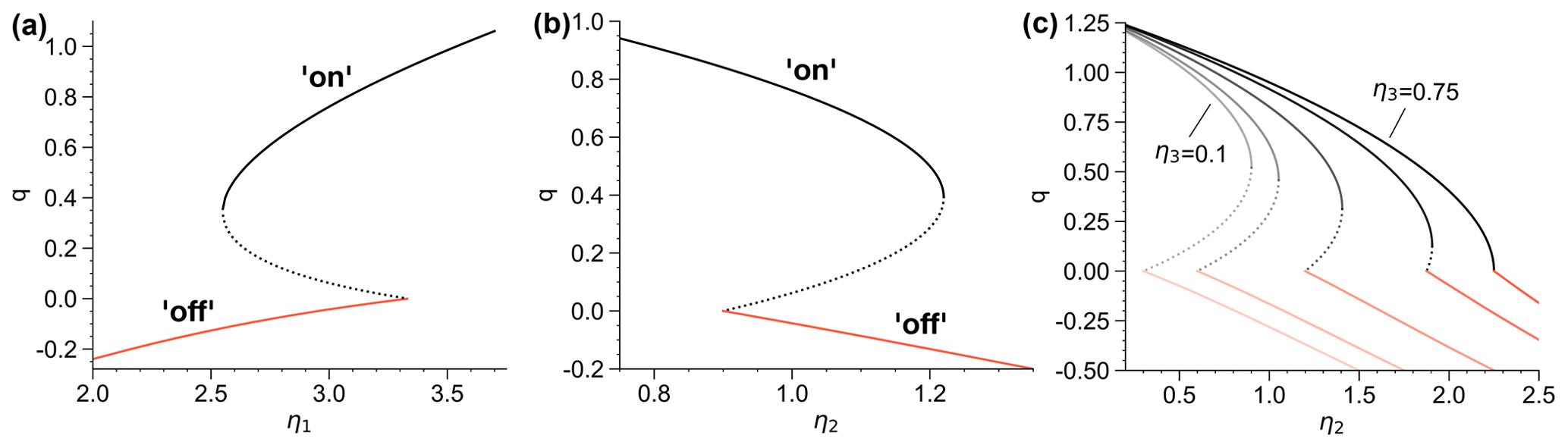
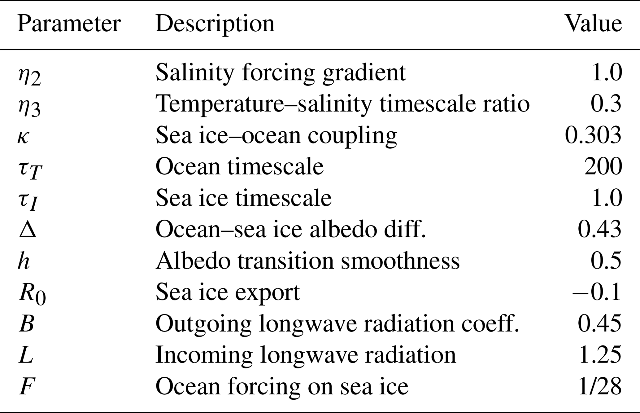
Figure 1 (a) Bifurcation diagram of the Stommel box model with η1 as control parameter, η2=1.0 and η3=0.3. Solid lines indicate branches of stable fixed points, whereas dotted lines indicate unstable fixed (or saddle) points. (b) Bifurcation diagram with η2 as control parameter, η1=3.0 and η3=0.3. (c) Dependence of bi-stability on η3 (η1=3.0). The individual bifurcation diagrams with η2 as control parameter are shown with decreasing bistability interval as η3 is increased from 0.1 up to 0.75.
2.1 Ocean component: Stommel's 1961 box model
We consider the Stommel box model of the Atlantic thermohaline circulation (Stommel, 1961) with added noise to represent variations in the atmospheric forcing on short timescales. The model assumes the overturning flow ψ in between well-mixed polar and equatorial ocean basins to be proportional to the density difference
where the density is given by the equation of state of seawater
with some reference densities, temperatures and salinities represented by ρ0, T0 and S0, respectively. The two model variables represent the dimensionless temperature difference and salinity difference in between the boxes. This defines the dimensionless overturning circulation strength
Temperature and salinity in the boxes relax towards an atmospheric temperature and salinity forcing and . The meridional difference of the forcing drives the circulation and is represented by the two parameters and . A third parameter represents the timescale ratio of the temperature and salinity relaxation . The model is then defined by the stochastic differential equations
with the Wiener processes WS,t and WT,t. Time is scaled with respect to the ocean timescale τT=200 years. For a more detailed derivation of the model, see Dijkstra (2008). The deterministic system features a parameter regime with two stable equilibria, which are referred to as the circulation “on” and “off” states. For the on state we have T>S, where the temperature forcing gradient dominates the opposing salinity forcing gradient and drives the circulation. The off state (S>T) corresponds to a reversed circulation, which is weaker and dominated by the salinity forcing gradient. In Fig. 1a and b we show deterministic bifurcation diagrams of q with respect to the parameters η1 and η2. In both cases, the on state loses stability in a regular saddle-node bifurcation, whereas the off state destabilizes in a non-smooth saddle-node bifurcation. The latter is also known as a non-smooth fold (di Bernardo et al., 2008) and is due to the fact that the Stommel model is a non-smooth dynamical system owing to the absolute value in its equations (see Sect. S3 and Fig. S3 for more detail). The existence and extent of bi-stability depends on the parameter η3. A large timescale separation (slower salinity damping) leads to a large region of bi-stability, whereas as the salinity damping approaches the timescale of temperature damping, the bistability disappears (Fig. 1c). This is because a faster salinity damping disables the positive salt advection feedback, which gives rise to the bi-stability.
2.2 Coupled sea ice–ocean model
The ocean model is coupled to a sea ice component in the polar ocean box, which is the energy balance model described in Eisenman and Wettlaufer (2009) and Eisenman (2012), modified by neglecting the seasonal cycle and effects of the sea ice thickness. The changing sea ice cover acts to insulate the polar ocean to varying degrees from the cold atmospheric temperature forcing , thus modulating the temperature forcing gradient . A schematic of the coupled model, including model variables and important parameters, is given in Fig. 2. The deterministic sea ice component is defined (Eisenman and Wettlaufer, 2009) by
with the Heaviside step function Θ(⋅). Time is scaled with respect to τI=1 year. The parameters and their values are described in Table 1. While I>0 corresponds to a positive sea ice cover, I<0 represents zero sea ice cover, and the variable is instead a measure of the enthalpy of the surface ocean (Eisenman, 2012). The control parameter R models influences on the sea ice concentration due to external factors, such as export or import of sea ice into the North Atlantic via changes in wind stress. While in the climate system R is driven by slower dynamic processes, such as changes in ice sheet topography, we treat it as a control parameter. We use parameter values from Eisenman (2012), which yield a sea ice component that is bi-stable with respect to R. As seen in Fig. 3, for a range of R there exists a stable state with a positive sea ice cover (red), as well as a state with zero sea ice cover I<0 (black). This range is bounded by two saddle-node bifurcations. The stable state with sea ice cover collapses at . We define the state at R=0 as the stadial state, yielding a fixed point with positive sea ice cover . A slight deviation from the parameters of Eisenman (2012) is our larger value of h, which gives a more gradual albedo transition from an ice-free to an ice-covered state. Accordingly, the bifurcation diagram is more “S-shaped” instead of “Z-shaped” (see Sect. S1 and Fig. S1 in the Supplement for more details).

Figure 2 Schematic of the coupled sea ice–ocean model including model parameters and variables (bold). A description of the parameters is given in Table 1. The well-mixed polar and equatorial ocean boxes are coupled by a surface flow q, along with an identical return flow at the bottom. The ocean component is reduced to the two variables and . In the polar ocean box, the sea ice cover I insulates the ocean from the cold atmospheric temperature .
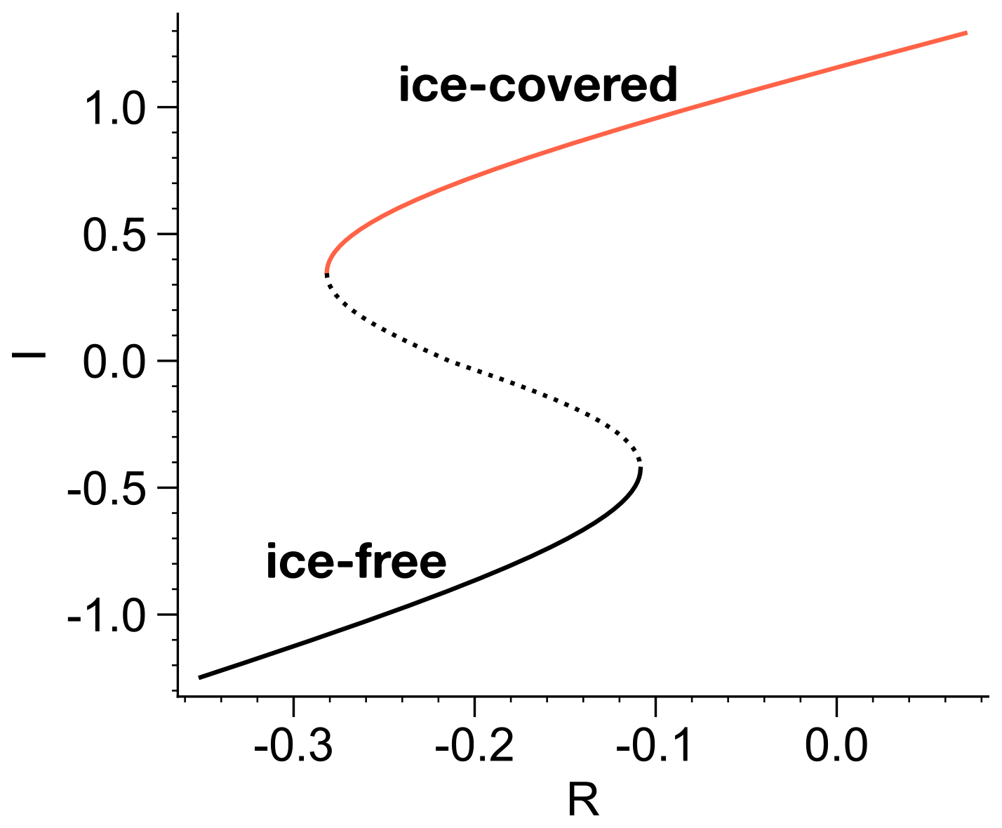
Figure 3 Bifurcation diagram of the sea ice component for parameter values as in Table 1. The solid (dotted) lines indicate stable (unstable) fixed points.
To model transitions from stadial to interstadial conditions in the coupled sea ice–ocean model, we consider the following mechanism. The glacial polar ocean is insulated by a high sea ice concentration from the atmospheric temperature forcing, preventing it from losing heat efficiently. As the sea ice concentration decreases, the polar ocean becomes more and more exposed to the cold atmosphere and loses heat. Thus, the sea ice variable modulates the parameter η1, which we now define as , with the Heaviside function Θ(⋅) since I<0 corresponds to zero sea ice cover. Adding noise as a model of fast atmospheric perturbations (Wiener process WI,t), this yields the following coupled equations:
The value of κ reflects the change in atmospheric temperature forcing when removing the sea ice cover. In this conceptual framework it can only be chosen heuristically. We can for instance assume for an open ocean, and atmospheric temperature forcings in a glacial climate of 20 and −10 ∘C in the equatorial and polar box, respectively. Full sea ice cover would limit the polar temperature forcing to 0 ∘C, corresponding to η1=2.0. Even if the glacial polar atmosphere were above 0 ∘C, given that it was colder than the surface ocean, extensive sea ice cover would severely reduce heat loss to the atmosphere and thus effectively reduce η1. Here we choose a scenario where during the stadial the sea ice reduces the atmospheric forcing from η1=3.0 to η1=2.65. κ is then chosen such that η1=2.65 at the stadial fixed point and η1=3.0 for I<0, yielding . As a result, the ocean component is in the bi-stable regime for both full and zero sea ice cover. A transition from stadial to interstadial will then be captured by decreasing R from zero beyond the bifurcation point, which tips the sea ice component towards a state of I<0, while the ocean remains in the bi-stable regime.
Due to the unidirectional, linear coupling of the model, and our focus on a specific dynamical regime, we restrict our presentation of the coupled dynamics to the individual bifurcation diagrams of the sea ice component with R as control parameter and of the ocean component with η1(I) as effective control parameter. The full bifurcation structure of the coupled model with R as the only control parameter is presented in Sect. S2 and Fig. S2.
3.1 Rate-induced tipping and soft tipping points in the Stommel model
Here we investigate the tipping dynamics in the ocean component in the deterministic limit (). As noted above, there is a non-smooth fold in the Stommel model as the off state loses stability, which leads to a resurgence of the AMOC. In the bifurcation diagrams of Fig. 4 it can be seen that, both in terms of T and S, the stable fixed point (red line) moves in the same direction as the saddle point when the non-smooth fold bifurcation is approached. Thus, in a sufficiently fast parameter shift towards the fold, the saddle point can outpace the system state, which is trying to follow the moving equilibrium. This is illustrated in Fig. 4, where instantaneous parameter shifts and the corresponding movements of the system state vector in the bifurcation diagrams are indicated. When the saddle point moves past the system state, the system will tip towards the alternative stable state, which is the on circulation in our case. Thus, tipping can occur even before the bifurcations points are reached, which is known as rate-induced tipping. While in the Stommel model this can happen for both η1 and η2 as control parameter, it occurs for a larger range of amplitudes and rates of the parameter shift when changing η1.
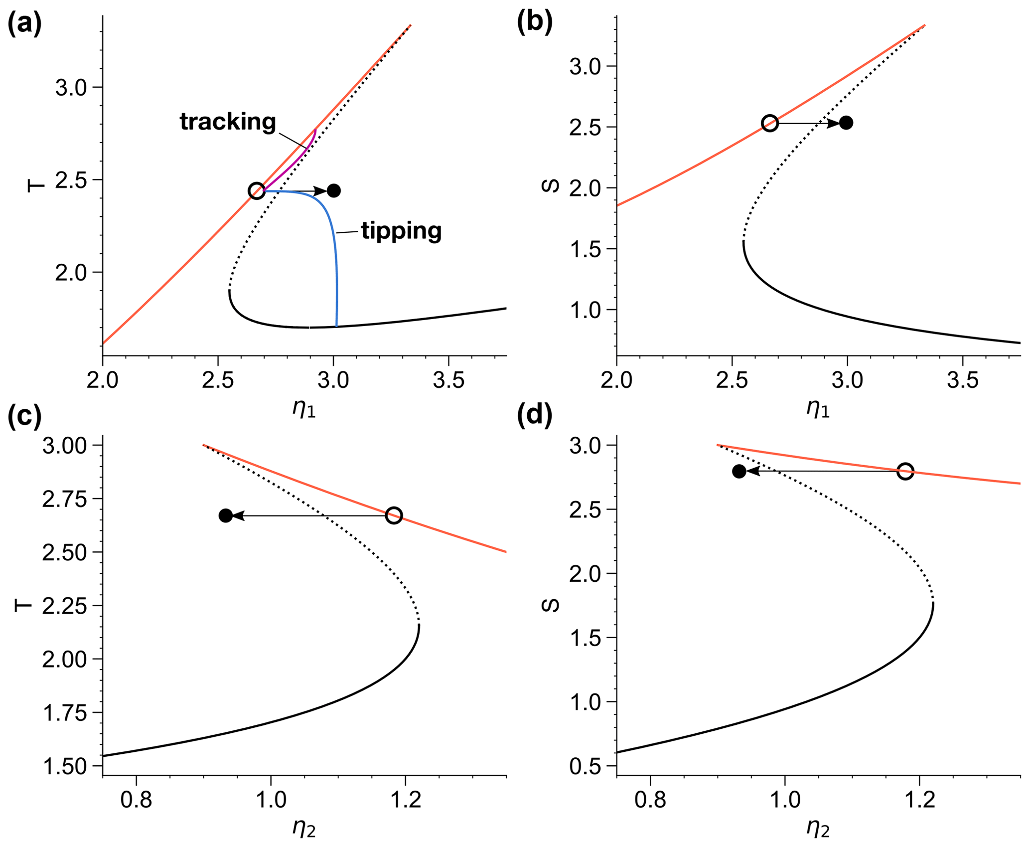
Figure 4 (a, b) Bifurcation diagram of the Stommel model equilibria in terms of the variables (a) T and (b) S as a function of η1 as control parameter with η2=1.0 and η3=0.3. (c, d) The same as (a, b) but with η2 as control parameter with η1=3.0 and η3=0.3. Solid lines indicate stable fixed points, whereas dotted lines indicate saddle points. The horizontal arrows indicate the movement of the system state as the control parameter is changed instantaneously within the bi-stable regime. In (a) we illustrate how the system state may track the moving equilibrium for a slow parameter shift (purple trajectory) or tip to the undesired equilibrium in a fast parameter change (blue trajectory).
To be more rigorous one has to consider the movement of the basin boundary as the control parameter is changed. The basin boundary is the stable manifold of the saddle, and it separates the basins of attractions of the on and off states, i.e., the sets of initial conditions that converge to the respective attractors. In Fig. 5 we illustrate the movement of the fixed points and basin boundary as η1 is changed from 2.65 to 3.0. This corresponds to the scenario of a transition from stadial to interstadial sea ice cover in the coupled model, as described in Sect. 2.2. Figure 5b shows that the off fixed point before the parameter shift (open circle) lies inside the basin of attraction of the on fixed point after parameter shift (blue area). This is a sufficient condition for rate-induced tipping, which has been called basin instability (O'Keeffe and Wieczorek, 2020), since for an instantaneous parameter shift, the system would tip to the other attractor. Similarly, as the system tries to follow the moving fixed point during a sufficiently fast parameter shift, it will fail to reach the off basin (orange area) at the end of the parameter shift and tip to the on fixed point. This happens for the blue trajectory, where the parameter is ramped up linearly within 300 years. In contrast, the purple trajectory shows that tipping does not occur for a ramping duration of 500 years. For this given amplitude of the parameter shift, there is a critical rate of parameter change in between these two values.
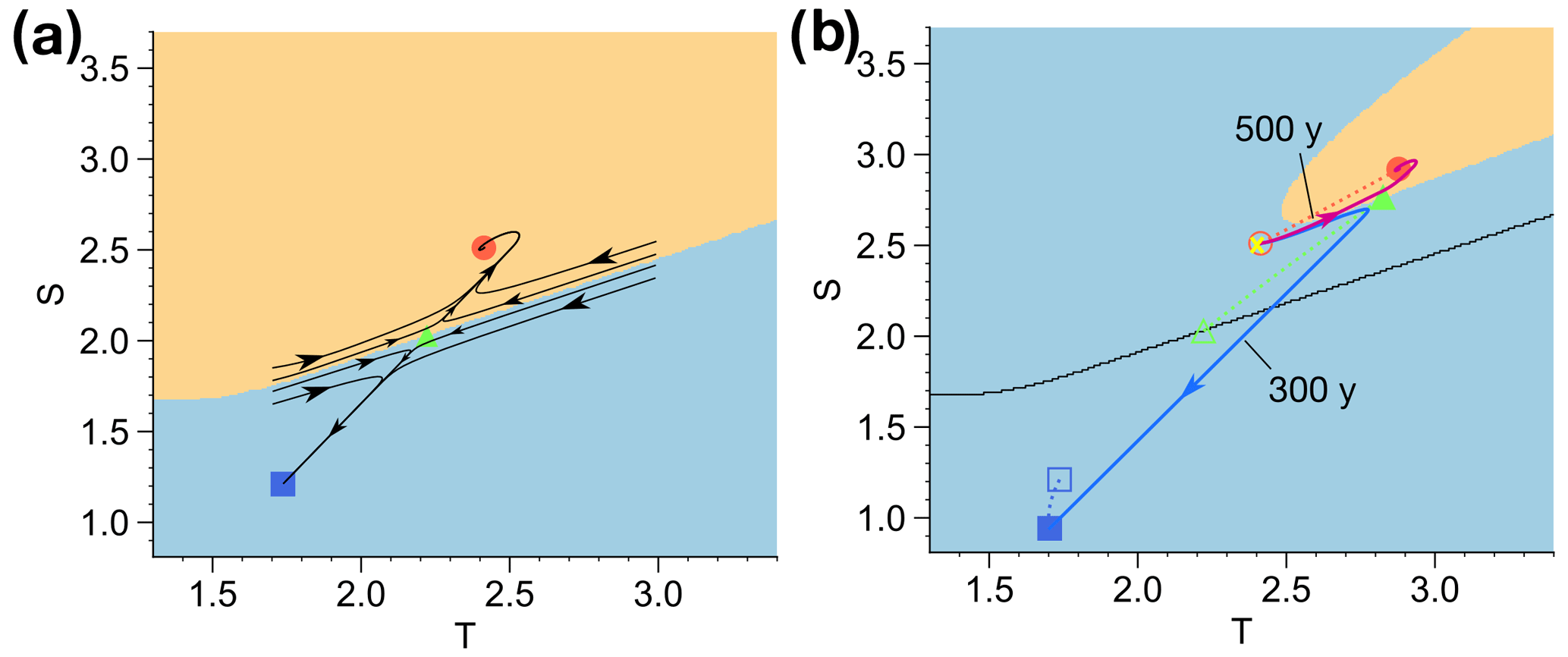
Figure 5 Phase portraits of the Stommel model with basins of attraction and fixed points. Squares and dots indicate stable fixed points, and triangles denote saddle points. (a) Phase portrait for η1=2.65 with several flow lines to indicate the dynamics around the saddle. The basin of attraction of the off (on) state is shaded in orange (blue). (b) Phase portrait for η1=3.0. Two trajectories where η1 is ramped linearly from η1=2.65 to η1=3.0 within 300 and 500 years are shown in blue and purple, respectively. The initial conditions are indicated by the yellow cross. Open symbols indicate the positions of the fixed points at η1=2.65, and the black curve indicates the corresponding basin boundary from (a).
Figure 6 shows time series of q for simulations with different ramping durations. The realizations in Fig. 6a and b tip to the on attractor, while the realizations in Fig. 6c and d track the moving off equilibrium. The critical ramping duration is in between the 388.5 and 390 years employed in Fig. 6b and c. Comparing Fig. 6a to b, one observes a delay in the tipping in Fig. 6b of thousands of years. This occurs because, for close-to-critical rates, the system state passes by very closely to the saddle point, where it remains for a long time as the dynamics slow down before being ejected. The close approach of the saddle happens because the system state is attracted by the saddle's stable manifold, which is also the basin boundary. If one were to use the exact critical ramping duration, the system state would evolve precisely towards the saddle and remain there. Such trajectories are called maximum canards (O'Keeffe and Wieczorek, 2020). This behavior is also seen for trajectories that eventually track the moving equilibrium, as in Fig. 6c. It is worth noting that the attraction by the stable manifold of the saddle continues after the parameter shift is already over, as shown in the inset in Fig. 6c.
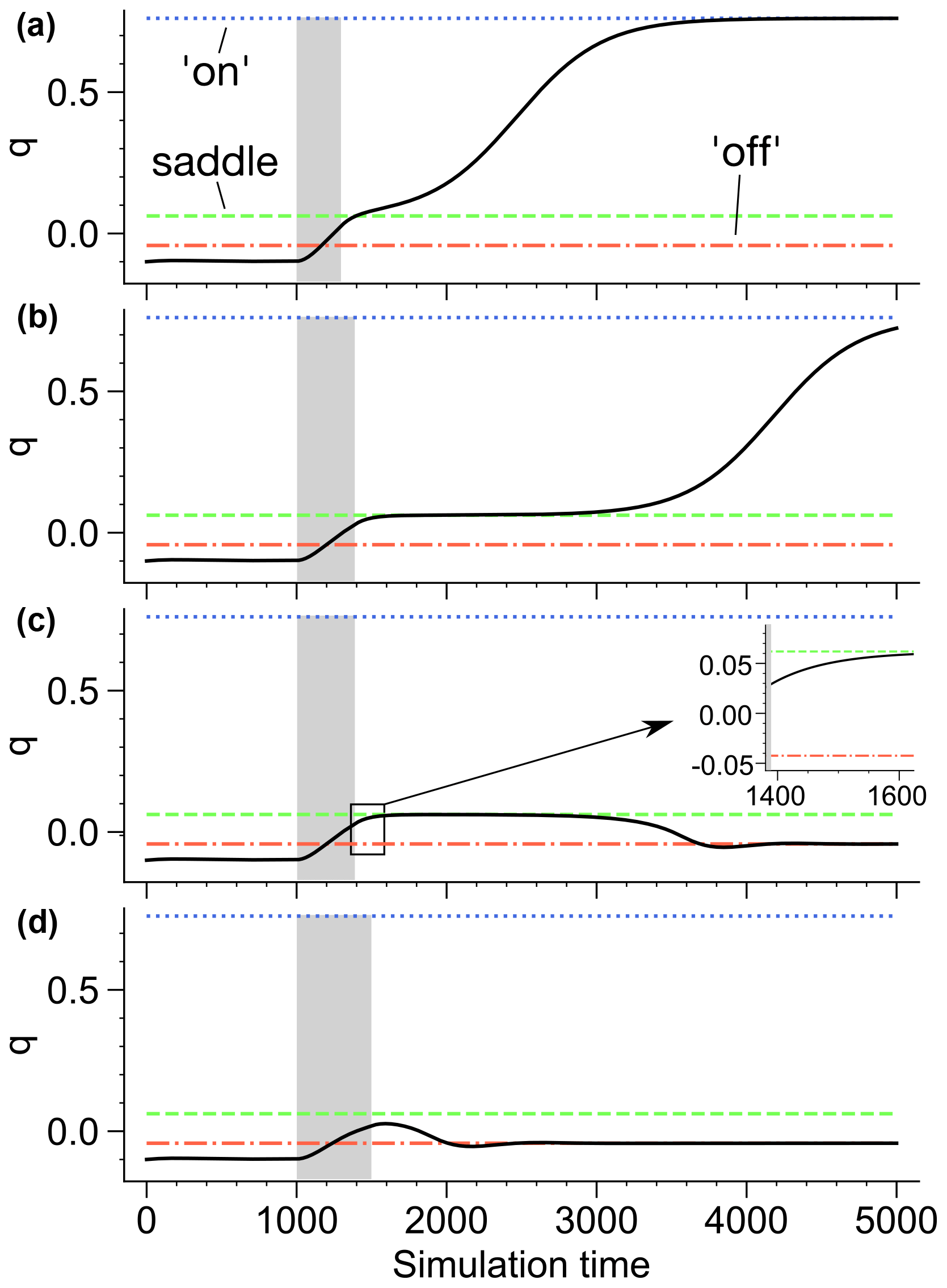
Figure 6 Time series of in the Stommel model when ramping the parameter from η1=2.65 to η1=3.0 at different rates. The realizations are initialized at , which is close to the off fixed point at η1=2.65. The duration of the ramping is indicated by the gray shading. The realizations in (a) and (b) with ramping durations of 300 and 388.5 years, respectively, tip from the off to the on attractor. The realizations in (c) and (d) with ramping durations of 389 and 500 years, respectively, track the moving off attractor. The on, off and saddle fixed points at η1=3.0 are shown as horizontal lines.
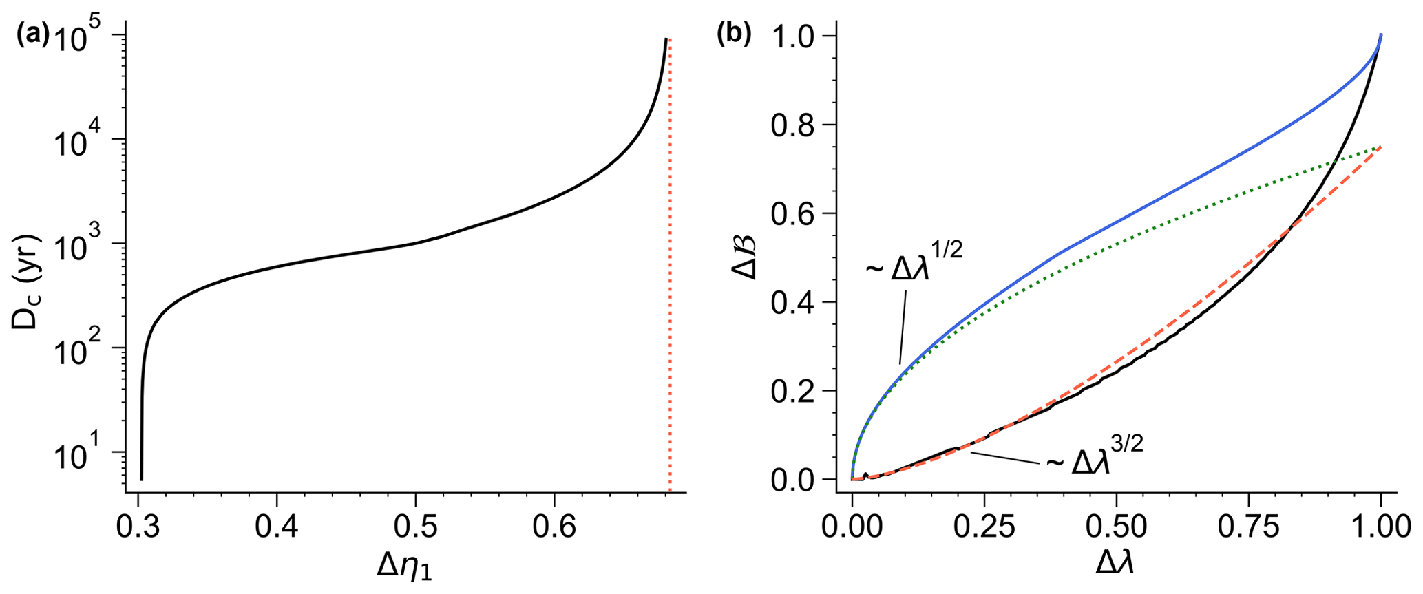
Figure 7 (a) Critical ramping duration below which there is a rate-induced tipping in the Stommel model when shifting the parameter from η1=2.65 to . The off attractor loses stability in the bifurcation at , as indicated by the dashed red line. (b) Normalized shortest distance to the basin boundary Δℬ as a function of the normalized distance to the bifurcation . is the parameter value at the other saddle node bifurcation of the on state. The solid black curve shows the results of the Stommel model, and a proposed super-linear scaling is shown by the dashed curve. Also shown are results for the smooth bifurcation in the sea ice component (solid blue) and the corresponding square-root scaling (dotted).

Figure 8 (a) Probability of a rate-induced tipping in the Stommel model from the off to the on state as a function of the linear parameter ramping duration from η1=2.65 to η1=3.00. Different noise levels are considered: σ=0.01 (lightest gray curve), σ=0.02, σ=0.04, σ=0.06, σ=0.1, σ=0.2, and σ=0.4 (darkest gray curve). The dashed red line is the critical ramping duration in the deterministic system. (b) Probability distributions of the time of tipping, defined by the first crossing of q>0.1, for different noise levels. The ramping is started in year 1000 and the duration is fixed at 300 years. The dashed red line is the time of tipping in the deterministic system.
The critical ramping duration depends on the amplitude Δη1 of the parameter shift (Fig. 7a). Rate-induced tipping becomes possible at a certain Δη1, where the basin instability condition is first satisfied. Increasing Δη1 then leads to a very rapid increase of the critical ramping duration Dc. Thereafter, Dc keeps increasing and actually diverges as the bifurcation is approached. This is due to the non-smoothness of the fold bifurcation, where the attractor and saddle meet in a cusp (see Sect. S3 and Fig. S3 for more detail). As a result, the attractor gets close to the basin boundary very quickly as the bifurcation is approached. This leads to a super-linear scaling of the shortest distance to the basin boundary. In Fig. 7b, we compare this to the square-root scaling of the smooth fold bifurcation in the sea ice component. In the non-smooth case, as the bifurcation is approached the basin boundary gets arbitrarily close to the attractor. Then, even very small and slow parameter increases lead to tipping. Thus, the non-smooth fold leads to what could be called a soft tipping point. In practice, there is no hard critical threshold of the parameter, but for any parameter shift at finite rate, the tipping will occur at some point prior to the bifurcation. The precise location of the tipping point depends on the trajectory of the parameter shift.
3.2 Noisy rate-induced tipping
We now consider additive noise in the ocean component, which models variations in atmospheric forcing on short timescales. In addition to the soft tipping just described, the stochastic perturbations further blur the critical threshold leading to tipping. For a given amplitude of the parameter shift, there is no longer a critical rate but a range of rates where the probability of tipping goes from 0 to 1. Figure 8a shows how this range of rates expands for increasing noise level. Note that since the system features unbounded noise, we consider finite time-tipping probabilities during a simulation time of 5000 years. Eventually, there will always occur a noise-induced transition to the on attractor, especially from the off attractor at η1=3.0 for higher noise levels.
By introducing noise, tipping becomes a mixture of rate-induced and noise-induced transitions, since the unbounded noise allows the system to cross the basin boundaries of the deterministic system in any circumstances. Still, for low noise levels the behavior strongly resembles the deterministic case. As discussed earlier, for a ramping speed relatively close to the critical rate, the tipping involves an escape from the saddle. This behavior is robust for low noise levels, where the stochastic fluctuations cannot overcome the attraction of the stable manifold of the saddle. Thus, the system approaches the saddle before being ejected from its vicinity.
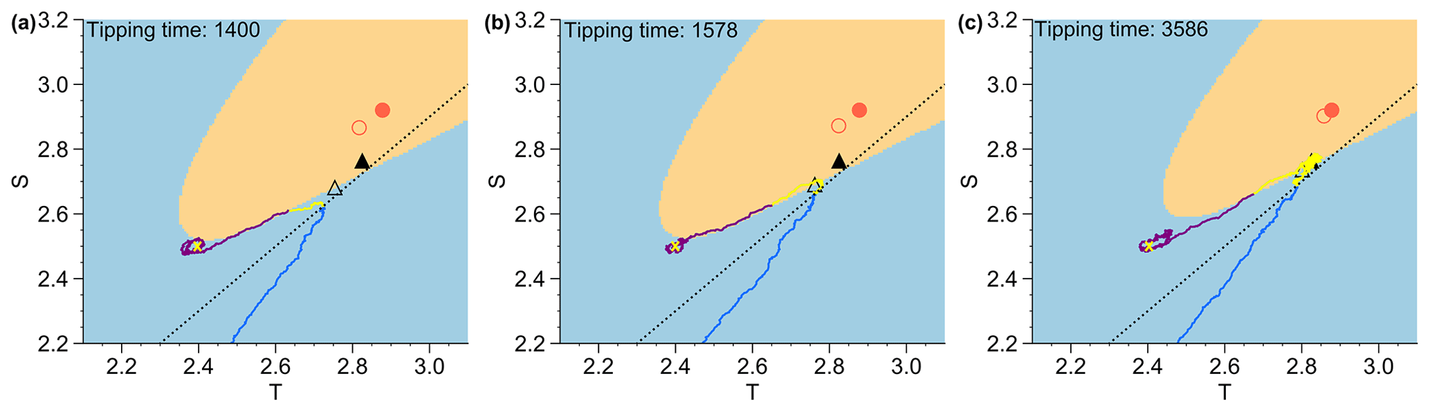
Figure 9 (a–c) Three realizations in phase space of the Stommel model with , where η1 is ramped from η1=2.65 to η1=3.00 over 300 years. The filled dot (triangle) marks the off fixed point (saddle) at η1=3.0. The colored areas are the quasi-stationary basins of attraction at the time when their boundary is first crossed. The colored basins of attractions are given at the time of first basin crossing of the trajectories, which change color from purple to yellow. The initial conditions are indicated by the yellow cross. The locations of the saddle point (triangle) and the on fixed point at this time are shown with open symbols. The threshold used to define the time of tipping is shown as a dotted line.
As the noise level is increased, there are noise-induced early tippings as well as significantly delayed tippings. In order to quantify when a tipping is “early” or “late”, we need to define the moment when the system actually tips. For the deterministic system, a sensible choice would be the time when the moving, quasi-stationary basin boundary is crossed, since this is the first moment that the system would tip in case the parameter shift would be stopped suddenly. However, for the noisy system this does not guarantee tipping, since the system may cross back to the other basin at any time. As a heuristic definition of tipping, we can instead detect the departure from the vicinity of the saddle in terms of the overturning q, as the tipping is associated with a monotonic increase of q (see Fig. 6). Thus, as tipping we define the first crossing of q=0.1, which is a slightly larger value than at the saddle to allow for some fluctuations around it. In phase space this defines a straight line.
Figure 9 shows the crossing of this threshold, as well as the basins at the time when the basin boundary is first crossed, for three different realizations with a ramping duration of 300 years and . The time of tipping varies significantly and depends primarily on the proximity of the approach to the saddle and the subsequent time spent in its vicinity. Whereas Fig. 9b shows a realization with tipping close to the deterministic scenario, the realization in Fig. 9a leaves the stable manifold early and does not approach the saddle closely. The realization in Fig. 9c approaches the saddle very closely and remains there for a long period of time.
The tipping time distribution and its dependence on the noise level is shown in Fig. 8b. In our case of a ramping duration slightly below the critical value of the deterministic system, there are three regimes of noise levels. For low noise (σ=0.01, σ=0.02, σ=0.04 and σ=0.06 in Fig. 8b) the trajectories are very similar to the deterministic case, and it is very unlikely that the noise pushes the system closer to the saddle. Thus, the tipping time is distributed closely around the deterministic value. For intermediate noise (σ=0.1 and σ=0.2 in Fig. 8b), some early noise-assisted tippings are possible, as seen by the shift of the distribution mode towards earlier times. For other realizations there is a good chance that the noise pushes the system closer to the saddle, where it can stay for a long time (thousands of years) as the dynamics slow down before escaping. This leads to the development of a long tail in the tipping time distribution. For larger noise (σ=0.4 in Fig. 8b), even earlier noise-assisted tippings are seen, as well as some delayed tippings. However, the latter do not occur as frequently as for intermediate noise since the average residence time at the saddle is also shortened.
3.3 Cascading dynamics
We now consider the coupled model and investigate how a stadial–interstadial transition can arise as a cascading tipping of the two components. The cascade is initiated by a change in the control parameter R leading to a decrease and eventual tipping of the sea ice to I<0. Subsequently, the modulation of the parameter η1(I) due to the decrease of I can be expected to induce a rate-induced resurgence of the AMOC. On the one hand, this is because the short sea ice timescale leads to very fast dynamics as the sea ice tips. On the other hand, even if the sea ice does not change quickly, when the amplitude of the change in η1(I) becomes larger, there will be rate-induced tipping anyway due to the soft tipping point in the Stommel model described earlier. We thus choose the robust scenario where the coupling κ is such that the ocean component remains in the bi-stable regime with respect to η1(I), and thus a rate-induced AMOC resurgence is the only pathway to tipping. As described in Sect. 2.2, this can be exemplified by a change in η1(I) from η1=2.65 (at the stadial sea ice fixed point for R=0) to η1=3.0 for a collapsed sea ice cover I<0. Simulations with these parameters are qualitatively representative for a wider range of coupling strengths and rates of changing R.
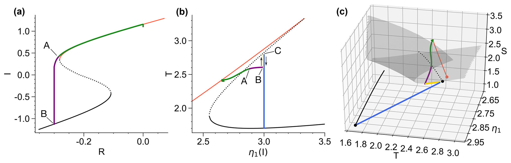
Figure 10 Cascading stadial–interstadial transition in the coupled sea ice–ocean model where R is ramped from R=0 to within 340 years and kept constant afterwards. (a) Trajectory of the sea ice component as function of the control parameter R. (b, c) Trajectory of the ocean component as function of the changing parameter . The tipping cascade consists of several steps separated by the points A, B, and C and marked by different colors in the trajectories (see main text). The gray surface in (c) is the moving basin boundary corresponding to the changing η1(I(t)).
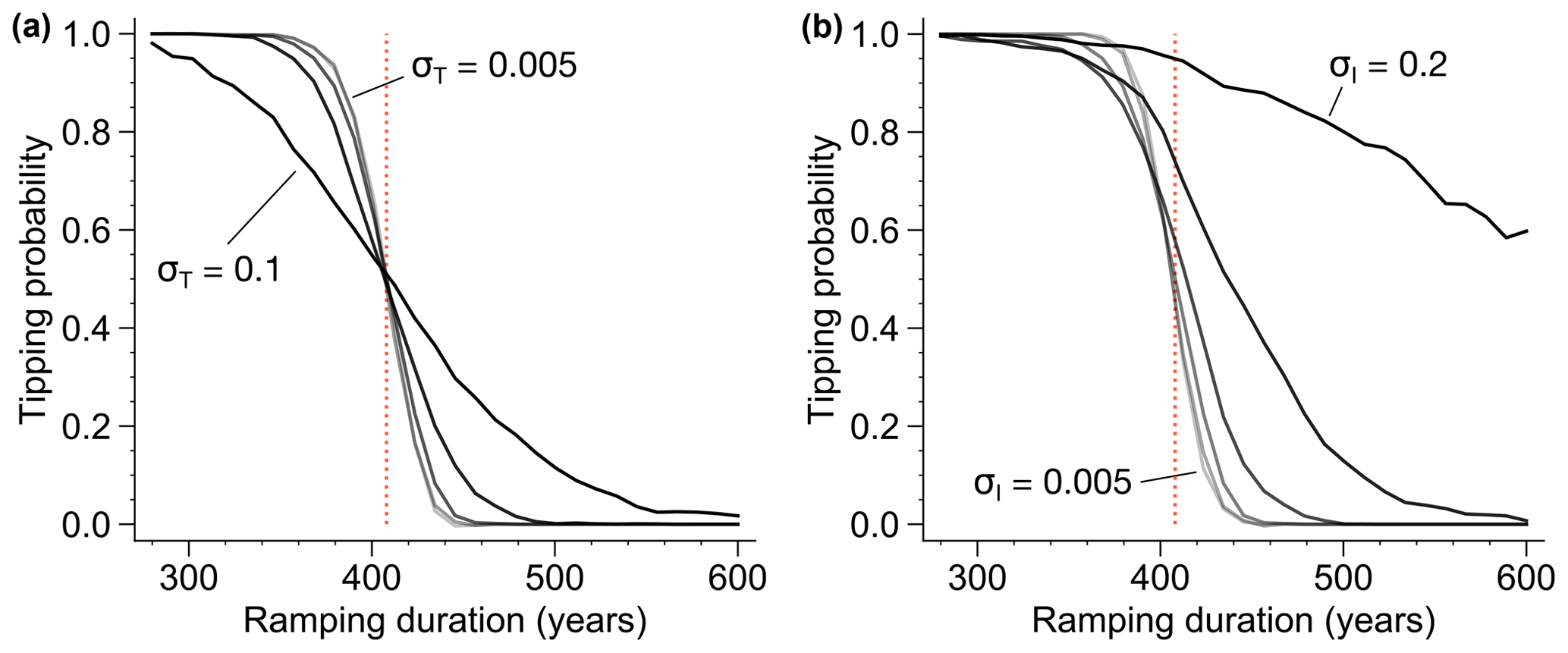
Figure 11 Probability of a cascading transition in the coupled sea ice–ocean model when changing the control parameter R linearly from R=0 to within different ramping times. (a) Fixed noise level σI=0.02 in the sea ice component and varying noise levels (lightest gray), σ=0.01, σ=0.02, σ=0.04 and σ=0.1 (darkest gray) in the ocean component. (b) Fixed noise level in the ocean component and varying noise levels σI=0.005 (lightest gray), σI=0.01, σI=0.02, σI=0.04, σI=0.08 and σI=0.2 (darkest gray) in the sea ice component.
Figure 10 shows trajectories for a cascading stadial–interstadial transition in the deterministic limit when R is ramped down from R=0 to over 340 years. The transition can be divided into several stages. First, the sea ice slowly decreases as R is decreased and the ocean component tries to track the moving equilibrium (green segment of trajectories in Fig. 10). At point A, 325 years after the start of ramping, the sea ice passes the bifurcation point and rapidly tips to I<0 (purple segment in Fig. 10). This leads to a quick movement of η1(I) towards η1=3.0, which is reached at point B, 350 years after the start of ramping (Fig. 10b). As a result, the ocean state crosses the moving basin boundary (gray surface in Fig. 10c) from above and is thus determined to undergo rate-induced tipping to the on attractor (solid black curve). However, before tipping the ocean state is attracted by the stable manifold (i.e., the basin boundary) of the saddle (yellow segment). Finally, at point C (700 years after the start of ramping) the ocean component escapes the vicinity of the saddle and tips towards the on state (blue segment).
There is a critical timescale below which such a cascading transition with a rate-induced tipping is possible. This is a combination of the rate of change in the control parameter R and the speed of the tipping of the sea ice, which is held fixed here. As additive noise is included in the model, the boundary of tipping in terms of the ramping time of the control parameter is again blurred. Figure 11a shows the tipping probabilities for different noise levels as a function of the ramping time of R. The result is very similar to the ocean-only case, except that because of the fast tipping in the sea ice, the average ramping times leading to tipping are slightly higher. The picture looks different as we increase the noise level in the sea ice component, as seen in Fig. 11b. Here, the ramping times that yield significant tipping probabilities simply increase with the noise level without a large simultaneous decrease of the tipping probability for lower ramping durations. This is because noise-induced transitions to I<0 occur before the bifurcation of I is crossed. Since these transitions happen on the fast sea ice timescale, a rate-induced tipping of the ocean model becomes possible even when R is changed very slowly. As in the ocean-only case, the tipping cascade involves a saddle escape, which can lead to significant tipping delays as noise forcing of intermediate strength is included. Next, we will discuss this in more detail and relate it to potential pre-cursor signals leading up to such transitions.
3.4 Early warning of the tipping cascade
Due to their irreversible nature, it is important to foresee impending tipping points using generic early warning signals that do not require detailed knowledge of the system dynamics. These are typically obtained from time series by estimating a statistical indicator in a sliding window with appropriate detrending (see Sect. S4). For bifurcation tipping, a system often exhibits critical slowing down, which can be measured by increasing variance and autocorrelation. In Fig. 12 we show these indicators estimated in a sliding window for the cascading transition in Fig. 10. As expected there is an increase in variance and autocorrelation of I leading up to the bifurcation (Fig. 12c and d). Because of the speed of the parameter shift necessary to induce the cascade, the increases in the indicators do not fully exceed the variability prior to the parameter shift but could still provide early warning with a reasonable skill. Due to the coupling one might expect a signature of the sea ice critical slowing down in the ocean component. This is not seen here (Fig. 12e and f), since increasing fluctuations due to the sea ice are small compared to the variability in the ocean component for the chosen σ. If no noise is added to the ocean variables, critical slowing down can be detected in T or S. This might be an example of scenarios proposed in Rypdal (2016) and Boers (2018), where it is hypothesized that a bifurcation in the sea ice system is detectable as increased variance in the high frequencies of ice core data prior to DO events. Similarly, the fluctuations in I of increasing amplitude and temporal correlation may influence the ocean subsystem in a more consistent way as the bifurcation is approached. This should increase the cross-correlation, especially on longer timescales that can be measured with detrended cross-correlation analysis (DCCA). This has been proposed as early warning indicator for cascading transitions (Dekker et al., 2018). The method is similar to detrended fluctuation analysis, but instead of scaling in the variance, it measures scaling in the covariance of two signals with increasing timescales (for details, see Zebende, 2011 or Dekker et al., 2018). We can detect a slight increase on average in the DCCA exponent of I and T (Fig. 12g) for the transition in Fig. 10. However, the increase found in individual time series is not statistically significant, owing to the large variance of the DCCA estimator.

Figure 12 Ensemble simulations of the coupled sea ice ocean model, where R is ramped linearly from R=0 to within 350 years. (a) Time series of R (dashed line) and mean time series of I with a 90 % confidence band of the ensemble (gray shading). (b) Mean time series and 90 % confidence band of T and S. (c–f) Indicators of critical slowing down for I and T, estimated in a sliding window of 150 years, where the data in the window is detrended by a cubic function. The data is cut as the bifurcation in I is crossed until after the last realization tips plus the sliding window length. (g) Detrended cross-correlation analysis (DCCA) exponent estimated from I and T.
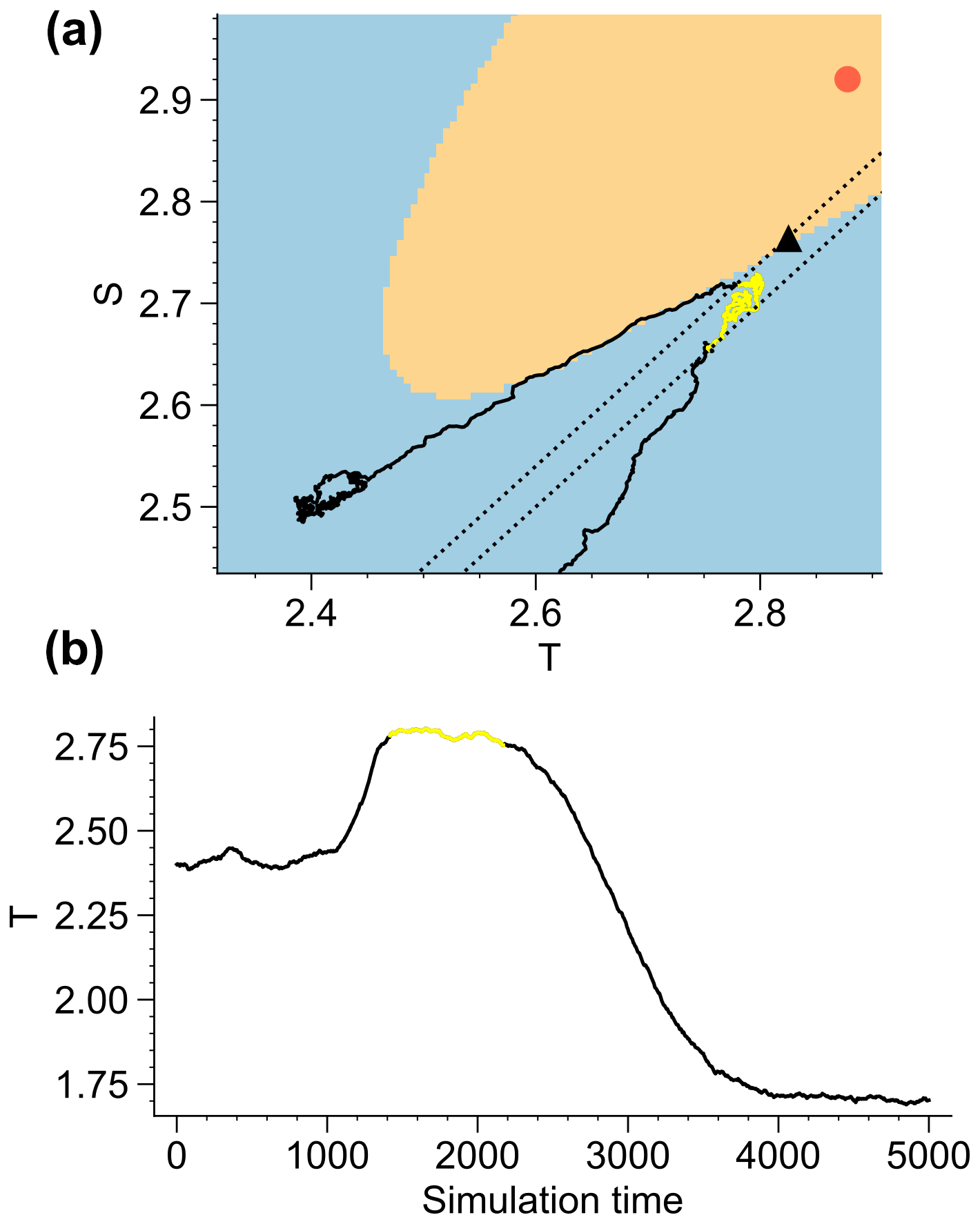
Figure 13 (a) Simulation in phase space of the Stommel model with , where η1 is ramped from η1=2.65 to η1=3.00 within 300 years. The two dotted lines correspond to the levels and . The trajectory in between the first crossing of these two thresholds is shown in yellow. (b) Corresponding time series of the variable T.
3.5 Early warning of rate-induced tipping in the Stommel model
During the rate-induced transition of the ocean component there is an increase in the ensemble variance, as can be seen by the shadings in Fig. 12b. This increase, as well as a corresponding increase in ensemble autocorrelation, has been proposed before as an early warning signal for rate-induced tipping (Ritchie and Sieber, 2016). However, we show here that this results from the large spread in the amount of time spent by individual realizations at the saddle before tipping to the other attractor (see Fig. 8). In contrast, the fluctuations in individual realizations, as used for operational early warning, do not show an increase in variance and autocorrelation. This can be seen in Fig. 12e and f, where no increases in sliding window variance and autocorrelation accompany the increase in ensemble variance. For the estimation of variance and autocorrelation in a sliding window, a detrending of the time series is necessary, such that remaining trends in the residuals are not larger than the fluctuations themselves. For our detrending method using cubic functions, the severity of detrending, and thus the ability to remove sharp changes in the signal trend, depends only on the sliding window size (see Sect. S4 for more details). In order to remove the trend due to the parameter shift regarded here, a window size of no more than 200 years is required (Fig. S4).
Detrending inevitably removes some of the original fluctuations. To show that the lack of increased fluctuations in the detrended time series is not a consequence of too severe detrending, we extract segments of time series simulated from the Stommel-only model, where the system is in the vicinity of the saddle and there are no sharp trends. The fluctuations around the saddle are then compared to time series segments where the system fluctuates around the initial attractor. We define the vicinity of the saddle by the time periods in the simulations where q=0.06 is first crossed until q=0.1 is first crossed (Fig. 13). We regard the time series segments of an ensemble of realizations where the system stays in this vicinity for at least a certain duration. After detrending the segments by cubic functions, we calculate variance and autocorrelation. This yields empirical distributions of these quantities, describing the fluctuations in the system shortly before tipping. For each realization, we also choose a segment of the same duration taken just before the parameter shift starts, yielding distributions of variance and autocorrelation at the initial attractor. Figure 14 shows that variance and autocorrelation at the saddle are not increased but actually slightly decreased compared to the initial attractor. This is best seen for longer segments (Fig. 14c and d), since there the uncertainty in the estimators is smaller. One can also see that in this case the average variance and autocorrelation are larger compared to Fig. 14a and b because the detrending in longer windows removes less variability on longer timescales.
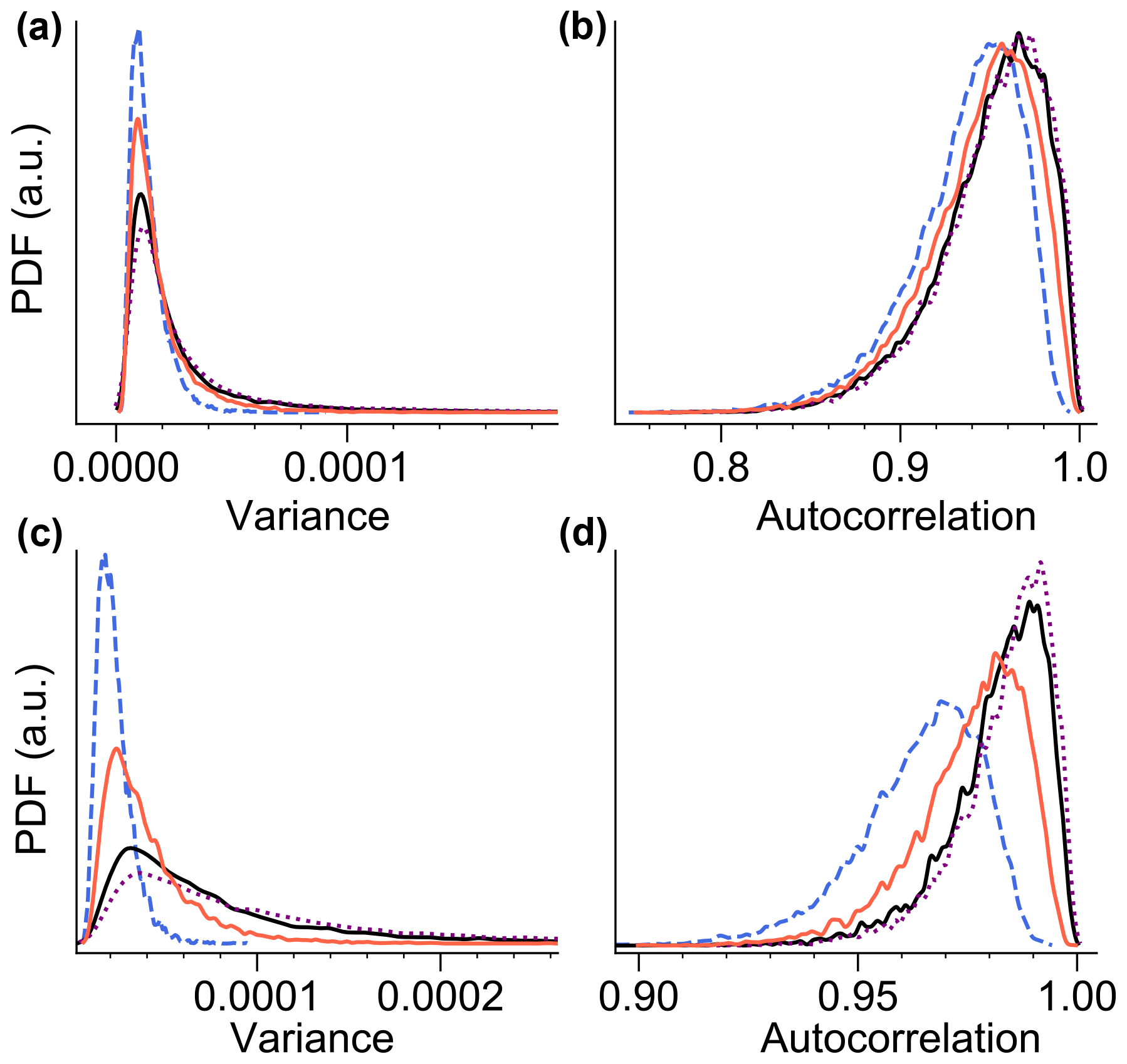
Figure 14 Distributions of variance and autocorrelation for ensembles of time series from the Stommel model (). These are estimated from time series segments around the initial fixed point at η1=2.65 (black) and close to the saddle point (orange; see main text). The length of the segments for each realization corresponds to the time period that the system spent in the vicinity of the saddle. (a, b) Results for realizations where these time windows were at least 300 years long. (c, d) Results for time windows of at least 700 years. Also shown are the distributions around the on attractor (dashed) and the off attractor at η1=3.0 (dotted).
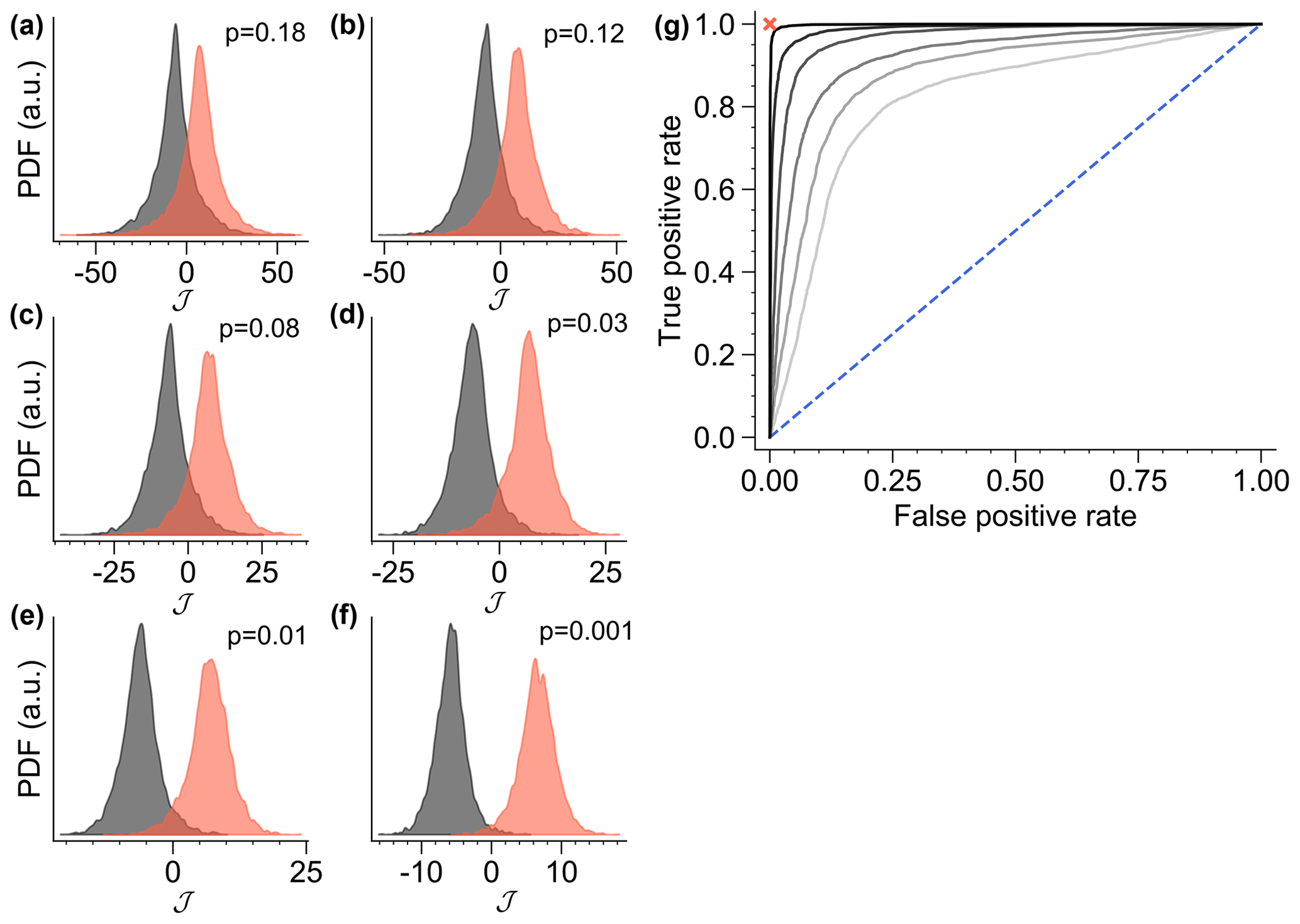
Figure 15 (a–f) Distributions of the early warning indicator 𝒥 for ensembles of time series from the Stommel model (), estimated around the initial fixed point at η1=2.65 (black) and close to the saddle point (orange). For each realization, 𝒥 is estimated after detrending in a time window that corresponds to the time period that the system spent in the vicinity of the saddle. In increasing order, the panels show results for realizations where these time windows were at least 100, 150, 200, 300, 400, and 600 years long, respectively. (g) Receiver operator characteristic curves for the same time series ensembles, showing the false and true positive rates as the threshold 𝒥c is increased from low (top right) to high values (bottom left). The increasing darkness in the gray scale of the curves corresponds to the increasing time window lengths, as above. The diagonal dashed line indicates the performance of a pure chance classifier. The red cross indicates a perfect classifier.
It thus does not appear that critical slowing down indicators apply to rate-induced tipping. Instead, we exploit that the system is attracted towards the saddle where the dynamics are different to those at the initial attractor. If this difference can be detected before the system tips, a small perturbation in the right direction or a reversal of the parameter shift could push the system back in the desired basin of attraction. Saddles, which have at least one unstable direction in phase space, can be distinguished from attractors by a change from a negative to a positive real part of the largest eigenvalue of the Jacobian. Estimating the Jacobian from the time series in a sliding window could thus be a generic tool to detect the saddle escape involved in rate-induced tipping, and we describe a method to do this in the Appendix A. With this method the elements of the Jacobian during rate-induced tipping of the Stommel model can be inferred and allow for the distinction of the dynamics around the different fixed points (Fig. S5). However, there are quantitative biases in the estimates of individual elements, and as a result the estimates of the real part of the largest eigenvalue in the vicinity of the saddle are not consistently positive. These biases could be a result of the detrending, of a too high noise level or because the unstable dynamics are “suppressed” since we consider time series segments taken before the escape from the saddle.
As a more reliable indicator we propose the actual elements of the Jacobian, since they are inferred in a qualitatively robust way (Fig. S5). This lowers the estimator variance compared to the eigenvalues, which are composed of the estimates of all elements. The off-diagonal elements record changes in sign of the feedbacks in between the system variables. Such changes in feedback are common as a system moves towards a saddle. We combine the off-diagonal elements to a scalar early warning indicator 𝒥, as defined in Eq. (A6). Figure 15a–f shows that 𝒥 can distinguish the dynamics around the attractor (black) and the saddle (red) before tipping. The panels correspond to different minimum lengths of the time windows used to estimate 𝒥. The figure also shows probabilities p of observing a value of 𝒥 estimated around the attractor that is larger than a value of 𝒥 in the vicinity of the saddle. This measures the performance of 𝒥 as an early warning signal. For longer time windows, the distributions become better separated since the uncertainty of the estimator is reduced. Still, even for relatively short windows the indicator correctly identifies the departure from the attractor for most realizations.
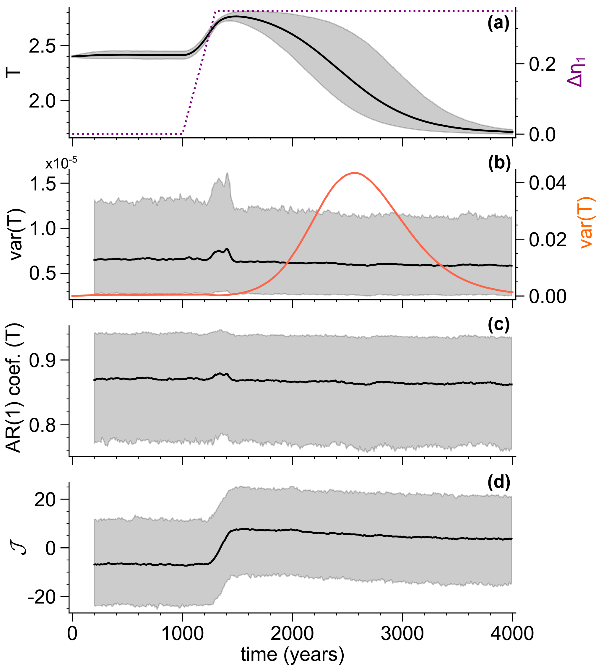
Figure 16 Early warning indicators estimated in a 200-year sliding window from an ensemble of time series of the Stommel model, where η1 is ramped from η1=2.65 to η1=3.0 within 300 years. (a) Time series of T and the parameter ramp. (b) Variance estimated from the detrended time series, as well as the ensemble variance (orange). (c) Lag 1 autocorrelation in the sliding window. (d) Early warning indicator 𝒥 (Eq. A6) estimated from the Jacobian in the sliding window. Mean time series are shown in black and the range in between 5th and 95th percentiles are shaded in gray.
An operational early warning signal can be constructed by estimating 𝒥 in a sliding window, and raising an alert as soon as a threshold 𝒥c is exceeded. Choosing a location of 𝒥c relative to the tails of the distributions in Fig. 15a–f is a trade-off in between maximizing the rate of true positives and minimizing the rate of false positives (alerts). The performance of the alert as a binary classifier can be summarized in receiver operating characteristic (ROC) curves. The curve of a perfect classifier collapses to the point (0,1). Figure 15g shows that for realizations that spend a longer time at the saddle, the indicator 𝒥 comes close to a perfect classifier, detecting the saddle approach with very low false positive and very high true positive rates. Figure 16 shows 𝒥 estimated from time series in a sliding window, along with critical slowing down indicators. 𝒥 begins to rise sharply roughly 200 years after the ramping started and decreases slightly as most realizations leave the saddle towards the on attractor. In contrast to the ensemble variance (orange), the variance and autocorrelation in the sliding window show no signal, apart from a small artifact around the parameter shift, which is a remnant of imperfect detrending in the 200-year windows.
In this work we propose a conceptual model that describes a mechanism for abrupt climate change comprising a rate-induced resurgence of the AMOC as a response to increasing atmosphere–ocean heat exchange, which results from fast disappearance of sea ice. The latter occurs via a bifurcation tipping as a response to changing sea ice export into the North Atlantic, which could be driven by changes in wind stress forcing due to variations in ice sheet topography. In the context of DO events, the proposed model merely describes the sequence of events leading to a stadial–interstadial transition and not the dynamics of entire DO cycles that repeat in a self-sustained way. The model omits processes on longer timescales, as well as processes that would initiate after the resurgence of the AMOC. However, it can be easily extended to display self-sustained DO cycles by adding another slow variable that dynamically models the parameter shift. This could be a simple negative feedback reflecting, e.g., the influence of the AMOC on the ice sheets. Similarly, stronger noise forcing of the sea ice together with a weak feedback from the ocean to the sea ice can yield an excitable system with stochastically driven DO cycles. The proposed mechanism is thus a dynamical skeleton that is in principle compatible with stochastic, externally forced and self-sustained oscillatory dynamics driving DO cycles. Whether it indeed played a role in past abrupt climate change remains to be confirmed with more complex models, as well as with analyses of new highly resolved and synchronized climate proxy records.
The type of cascade introduced here could be a common feature in coupled systems that feature multistability and timescale separation. Here, a tipping in a fast subsystem can trigger a rate-induced transition of a slower subsystem even for weak coupling. Conversely, when there is no timescale separation but stronger coupling, the cascade can still occur in systems with non-smooth fold bifurcations. This is due to soft tipping points (Sect. 3.1), where the critical ramping duration to enable rate-induced tipping diverges as the parameter shift increases towards the bifurcation point. As a result, the cascading dynamics seen in the conceptual model may also be relevant for other regime shifts in the climate system, as well as for other natural systems. Consequently, we examined the mathematical details of the tipping cascade, which occurs in several stages. During the parameter shift the ocean subsystem tries to track the moving equilibrium. As the sea ice component tips abruptly, this fails and the system is instead attracted by the stable manifold of the saddle. The system then remains in the vicinity of the saddle as the dynamics slow down, before escaping to the on attractor. Adding noise leads to a broad distribution of the tipping time towards the on attractor. Early tipping, where stochastic perturbations push the system away from the stable manifold, is observed as well as significantly delayed tipping. In the latter case, noise pushes the system very close to the saddle, where it can get stuck for a very long time. A similar delay of rate-induced tipping for low noise levels has been reported for a one-dimensional gradient system (Ritchie and Sieber, 2016). It is seen from our model that due to the attraction by the stable manifold of the saddle, the tipping delay is a robust feature that exists for a fairly large range of rates (both sub- and super-critical) and noise levels. Thus, it opens up the possibility of issuing an early warning for rate-induced transitions.
The main difficulty for achieving an early warning of the cascade before the initial tipping of the sea ice is due to the relatively fast parameter shift involved. Thus, indicators proposed for cascading tipping points (Dekker et al., 2018) yield non-significant results, and more research is needed to find better indicators that might rely on similar principles. Instead, we focused on the rate-induced tipping of the ocean subsystem, since early warning signals for rate-induced tipping have not been developed. As in the case of fast passages through a bifurcation, for very fast parameter shifts one cannot hope for an early warning of rate-induced tipping. Here the system is not attracted by the saddle but evolves quickly towards the alternative attractor. However, for intermediate rates we can exploit the fact that tipping occurs via saddle escape. As the system state departs from the moving attractor towards the saddle, the linear stability changes. This can be captured by the Jacobian matrix, which we estimate from the time series. We then propose using the off-diagonal elements of the Jacobian as an early warning signal. These elements record changes in the sign of coupling in between the system variables, indicating a change in stability. The proposed indicator detects an approach of the saddle with significant skill, in particular for realizations where the system stays in the vicinity for a longer time, so that the Jacobian can be estimated with good precision. Note that the actual tipping occurs by escaping the vicinity of the saddle, which is largely noise-induced. Thus, early warning in the sense of predicting the precise time of the saddle escape is hard to achieve. Early-warning signals for saddle escapes have been proposed (Kuehn et al., 2015), but they require being very close to the saddle and very low noise. While the specific early warning signal proposed here may not apply to all cases of rate-induced tipping, the general procedure of detecting a qualitative change in the feedback structure of the system via the Jacobian or its eigenvalues should be widely applicable. For higher-dimensional systems early warning might even become easier, since there are often dominant eigenvalues and large differences in the effective dimensionality of the dynamics on the attractor vs. the transient dynamics during tipping. Other techniques for detecting transient dynamics may also be useful here (Gottwald and Gugole, 2020). The phenomenology of cascading transitions involving rate-induced tipping that has been exemplified here is to be tested with models of different complexity in upcoming studies. Furthermore, the applicability of the early warning method to real-world data needs to be tested. In the typical case where only one (or a few) scalar time series are available, this will involve a time series embedding and subsequent estimation of the Jacobian from the reconstructed multivariate time series.
Building on previous studies of proxy records and state-of-the-art climate models, we propose that past abrupt climate change could have arisen as a cascade of tipping points. We translate this into a conceptual sea ice–ocean model, where a parameter shift leads to the following cascade. First, as a result of the gradually changing climatic conditions, the North Atlantic sea ice cover collapses abruptly. Subsequently, the AMOC resurges abruptly from a weak to a vigorous state in a rate-induced tipping, as a response to the fast rate of sea ice decline enhancing the atmosphere–ocean heat exchange. Our analysis suggests that cascades of tipping points in weakly coupled climate components with timescale separation become more likely under certain circumstances. This is the case when there are rate-dependent tipping points or soft tipping points associated with non-smooth fold bifurcations. This motivates the development of specialized early warning signals for such rate-dependent cascading tipping points. We present a first step in this direction by showing that due to a delay in the tipping of the ocean circulation a statistical estimation of the Jacobian can detect the impending abrupt transition. This may be applicable as generic early warning signal of rate-induced transitions.
We detect rate-induced tipping by identifying a departure from the initial attractor towards the vicinity of the saddle. This is accompanied by a change in the linear stability of the system and thus the Jacobian. The latter is estimated from the multi-variate time series in a sliding window as follows. Consider the underlying dynamical system with x∈ℝd and the observed discrete time series , where N is the window size. The linearization of the dynamical system around the equilibrium point y is
with . Discretized, this can be approximated as
In this expression, the factors are the elements Jji of the Jacobian matrix. They can be estimated with multiple linear regression by sampling different Δxt as a dependent variable and for i=1 … d as independent variables for a given y from within the time series. To this end, we choose from within the windowed time series, which are the M closest points to y in phase space in terms of the distance . For each x(tk), we evaluate using the subsequent point in the time series. From the M samples of and for i=1…d, we obtain the factors by multiple linear regression. We then repeat the procedure for every data point in the window as y, and average the results to obtain average Jacobian elements Jji within the sliding window. In this work we chose . To illustrate how the Jacobian changes in the Stommel model as the system departs the off attractor, we write Eq. (4) in the deterministic case as
The corresponding Jacobian of the linearized system is as follows.
Around the attractors, the real parts of both eigenvalues are negative. As the saddle is approached by crossing q>0, the real part of the first eigenvalue becomes positive. Furthermore, the off-diagonal elements of the Jacobian change sign. We propose this sign change as early warning signal, since it is more robust than the eigenvalues when estimated from noisy data. We define the early warning signal as
Note that for dynamical systems defined by a gradient of a potential this indicator is not applicable, since it would be 0 in the whole phase space due to the symmetric Jacobian. Using just one of the diagonal elements as indicator instead still gives good early warning possibilities with roughly half the statistical power due to the smaller amount of information retained. For time series from unknown dynamical systems, changes in the individual elements could be monitored simultaneously, potentially after embedding in the case of univariate time series.
The underlying software code of the model simulations is available at https://doi.org/10.5281/zenodo.5137364 (Lohmann, 2021).
The research data underlying the study have been created by simulation with the scripts in Code availability.
The supplement related to this article is available online at: https://doi.org/10.5194/esd-12-819-2021-supplement.
All authors contributed to the design of the research and interpretation of the results. JL performed the research and wrote the paper.
The authors declare that they have no conflict of interest.
Publisher's note: Copernicus Publications remains neutral with regard to jurisdictional claims in published maps and institutional affiliations.
This research has been supported by the Horizon 2020 (grant nos. TiPES (820970) and CRITICS (643073)) and the Villum Fonden (grant no. 17470).
This paper was edited by Christian Franzke and reviewed by two anonymous referees.
Ashwin, P., Wieczorek, S., Vitolo, R., and Cox, P.: Tipping points in open systems: bifurcation, noise-induced and rate-dependent examples in the climate system, Philos. T. R. Soc. A, 370, 1166–1184, 2012. a
Bevis, M., Harig, C., Khan, S. A., Brown, A., Simons, F. J., Willis, M., Fettweis, X., van den Broeke, M. R., Madsen, F. B., Kendrick, E., Caccamise II, D. J., van Dam, T., Knudsen, P., and Nylen, T.: Accelerating changes in ice mass within Greenland, and the ice sheet's sensitivity to atmospheric forcing, P. Natl. Acad. Sci. USA, 116, 1934–1939, 2019. a
Boers, N.: Early-warning signals for Dansgaard-Oeschger events in a high-resolution ice core record, Nat. Commun., 9, 2556, https://doi.org/10.1038/s41467-018-04881-7, 2018. a
Boers, N., Ghil, M., and Rousseau, D.-D.: Ocean circulation, ice shelf, and sea ice interactions explain Dansgaard–Oeschger cycles, P. Natl. Acad. Sci. USA, 115, E11005, https://doi.org/10.1073/pnas.1802573115, 2018. a
Cai, Y., Lenton, T. M., and Lontzek, T. S.: Risk of multiple interacting tipping points should encourage rapid CO2 emission reduction, Nat. Clim. Change, 6, 520–525, 2016. a
Dakos, V., Scheffer, M., van Nes, E. H., Brovkin, V., Petoukhov, V., and Held, H.: Slowing down as an early warning signal for abrupt climate change, P. Natl. Acad. Sci. USA, 105, 14308 –14312, 2008. a
Dansgaard, W., Johnsen, S. J., Clausen, H. B., Dahl-Jensen, D., Gundestrup, N. S., Hammer, C. U., Hvidberg, C. S., Steffensen, J. P., Sveinbjörnsdottir, A. E., Jouzel, J., and Bond, G.: Evidence for general instability of past climate from a 250-kyr ice-core record, Nature, 364, 218–220, 1993. a
Dekker, M. M., von der Heydt, A. S., and Dijkstra, H. A.: Cascading transitions in the climate system, Earth Syst. Dynam., 9, 1243–1260, https://doi.org/10.5194/esd-9-1243-2018, 2018. a, b, c, d
di Bernardo, M., Budd, C. J., Champneys, A. R., Kowalczyk, P., Nordmark, A. B., Tost, G. O., and Piiroinen, P. T.: Bifurcations in Nonsmooth Dynamical Systems, SIAM Rev., 50, 629–701, 2008. a
Dijkstra, H. A.: Dynamical Oceanography, Springer-Verlag, Berlin, Heidelberg, https://doi.org/10.1007/978-3-540-76376-5, 2008. a
Dokken, T. M., Nisancioglu, K. H., Li, C., Battisti, D. S., and Kissel, C.: Dansgaard-Oeschger cycles: Interactions between ocean and sea ice intrinsic to the Nordic seas, Paleoceanography, 28, 491–502, 2013. a
Eisenman, I.: Factors controlling the bifurcation structure of sea ice retreat, J. Geophys. Res., 117, D01111, https://doi.org/10.1029/2011JD016164, 2012. a, b, c, d
Eisenman, I. and Wettlaufer, J. S.: Nonlinear threshold behavior during the loss of Arctic sea ice, P. Natl. Acad. Sci. USA, 106, 28–32, 2009. a, b
Erhardt, T., Capron, E., Rasmussen, S. O., Schüpbach, S., Bigler, M., Adolphi, F., and Fischer, H.: Decadal-scale progression of the onset of DansgaardOeschger warming events, Clim. Past, 15, 811–825, https://doi.org/10.5194/cp-15-811-2019, 2019. a
Gottwald, G. A.: A model for Dansgaard–Oeschger events and millennial-scale abrupt climate change without external forcing, Clim. Dynam, 56, 227–243, 2021. a
Gottwald, G. A. and Gugole, F.: Detecting Regime Transitions in Time Series Using Dynamic Mode Decomposition, J. Stat. Phys., 179, 1028–1045, 2020. a
Heinrich, H.: Origin and Consequences of Cyclic Ice Rafting in the Northeast Atlantic Ocean During the Past 130,000 Years, Quaternary Res., 29, 142–152, 1988. a
Held, H. and Kleinen, T.: Detection of climate system bifurcations by degenerate fingerprinting, Geophys. Res. Lett., 31, L23207, https://doi.org/10.1029/2004GL020972, 2004. a
Henry, L. G., McManus, J. F., Curry, W. B., Roberts, N. L., Piotrowski, A. M., and Keigwin, L. D.: North Atlantic ocean circulation and abrupt climate change during the last glaciation, Science, 353, 470–474, 2016. a
IPCC: Special Report on the Ocean and Cryosphere in a Changing Climate, edited by: Pörtner, H.-O., Roberts, D. C., Masson-Delmotte, V., Zhai, P., Tignor, M., Poloczanska, E., Mintenbeck, K., Nicolai, M., Okem, A., Petzold, J., Rama, B., and Weyer, N., Cambridge University Press, Cambridge, UK and New York, NY, USA, 2019. a
Kleppin, H., Jochum, M., Otto-Bliesner, B., Shields, C. A., and Yeager, S.: Stochastic Atmospheric Forcing as a Cause of Greenland Climate Transitions, J. Climate, 28, 7741–7763, 2015. a
Klose, A. K., Karle, V., Winkelmann, R., and Donges, J. F.: Emergence of cascading dynamics in interacting tipping elements of ecology and climate, Roy. Soc. Open Sci., 7, 200599, https://doi.org/10.1098/rsos.200599, 2020. a
Kuehn, C., Zschaler, G., and Gross, T.: Early warning signs for saddle-escape transitions in complex networks, Sci. Rep.-UK, 5, 13190, https://doi.org/10.1038/srep13190, 2015. a
Lenton, T. M., Held, H., Kriegler, E., Hall, J. W., Lucht, W., Rahmstorf, S., and Schellnhuber, H. J.: Tipping elements in the Earth's climate system, P. Natl. Acad. Sci. USA, 105, 1786–1793, 2008. a
Li, C., Battisti, D. S., Schrag, D. P., and Tziperman, E.: Abrupt climate shifts in Greenland due to displacements of the sea ice edge, Geophys. Res. Lett., 32, L19702, https://doi.org/10.1029/2005GL023492, 2005. a
Lohmann, J.: Prediction of Dansgaard-Oeschger Events From Greenland Dust Records, Geophys. Res. Lett., 46, 12427–12434, 2019. a
Lohmann, J.: johannes-lohmann/cascading: cascadingv1.0 (Version v1.0), [code], Zenodo, https://doi.org/10.5281/zenodo.5137364, 2021. a
Lohmann, J. and Ditlevsen, P. D.: Risk of tipping the overturning circulation due to increasing rates of ice melt, P. Natl. Acad. Sci. USA, 118, e2017989118, https://doi.org/10.1073/pnas.2017989118, 2021. a
O'Keeffe, P. E. and Wieczorek, S.: Tipping Phenomena and Points of No Return in Ecosystems: Beyond Classical Bifurcations, SIAM J. Appl. Dyn. Syst., 19, 2371–2402, 2020. a, b
Ritchie, P. and Sieber, J.: Early-warning indicators for rate-induced tipping, Chaos, 26, 093116, https://doi.org/10.1063/1.4963012, 2016. a, b
Rocha, J. C., Peterson, G., Bodin, Ö., and Levin, S.: Cascading regime shifts within and across scales, Science, 362, 1379–1383, 2018. a
Rypdal, M.: Early-Warning Signals for the Onsets of Greenland Interstadials and the Younger Dryas–Preboreal Transition, J. Climate, 29, 4047–4056, 2016. a
Sadatzki, H., Dokken, T. M., Berben, S. M. P., Muschitiello, F., Stein, R., Fahl, K., Menviel, L., Timmermann, A., and Jansen, E.: Sea ice variability in the southern Norwegian Sea during glacial Dansgaard-Oeschger climate cycles, Sci. Adv., 5, eaau6174, https://doi.org/10.1126/sciadv.aau6174, 2019. a, b
Scheffer, M., Bascompte, J., Brock, W. A., Brovkin, V., Carpenter, S. R., Dakos, V., Held, H., van Nes, E. H., Rietkerk, M., and Sugihara, G.: Early-warning signals for critical transitions, Nature, 461, 53–59, 2009. a
Scheffer, M., Carpenter, S. R., Lenton, T. M., Bascompte, J., Brock, W., Dakos, V., van de Koppel, J., van de Leemput, I. A., Levin, S. A., van Nes, E. H., Pascual, M., and Vandermeer, J.: Anticipating Critical Transitions, Science, 338, 344–348, 2012. a
Stommel, H.: Thermohaline Convection with Two Stable Regimes of Flow, Tellus, XIII, 224–230, 1961. a
The IMBIE Team: Mass balance of the Greenland Ice Sheet from 1992 to 2018, Nature, 579, 233–239, 2020. a
Trusel, L. D., Das, S. B., Osman, M. B., Evans, M. J., Smith, B. E., Fettweis, X., McConnell, J. R., Noël, B. P. Y., and van den Broeke, M. R.: Nonlinear rise in Greenland runoff in response to post-industrial Arctic warming, Nature, 564, 104–108, 2018. a
Vettoretti, G. and Peltier, W. R.: Thermohaline instability and the formation of glacial North Atlantic super polynyas at the onset of Dansgaard-Oeschger warming events, Geophys. Res. Lett., 43, 5336–5344, 2016. a
Weijer, W., Cheng, W., Drijfhout, S., Fedorov, A. V., Hu, A., Jackson, L. C., Liu, W., McDonagh, E. L., Mecking, J. V., and Zhang, J.: Stability of the Atlantic Meridional Overturning Circulation: A Review and Synthesis, J. Geoph. Research, 124, 5336–5375, 2019. a
Wieczorek, S., Ashwin, P., Luke, C. M., and Cox, P. M.: Excitability in ramped systems: the compost-bomb instability, P. R. Soc. A, 467, 1243–1269, 2011. a
Wunderling, N., Gelbrecht, M., Winkelmann, R., Kurths, J., and Donges, J. F.: Basin stability and limit cycles in a conceptual model for climate tipping cascades, New J. Phys., 22, 123031, https://doi.org/10.1088/1367-2630/abc98a, 2020. a
Zebende, G. F.: DCCA cross-correlation coefficient: Quantifying level of cross-correlation, Physica A, 309, 614–618, 2011. a
Zhang, X., Lohmann, G., Knorr, G., and Purcell, C.: Abrupt glacial climate shifts controlled by ice sheet changes, Nature, 512, 290–294, 2014. a