Bayesian estimation of Earth's climate sensitivity and transient climate response from observational warming and heat content datasets

Future climate change projections, impacts, and mitigation targets are directly affected by how sensitive Earth's global mean surface temperature is to anthropogenic forcing, expressed via the climate sensitivity (S) and transient climate response (TCR). However, the S and TCR are poorly constrained, in part because historic observations and future climate projections consider the climate system under different response timescales with potentially different climate feedback strengths. Here, we evaluate S and TCR by using historic observations of surface warming, available since the mid-19th century, and ocean heat uptake, available since the mid-20th century, to constrain a model with independent climate feedback components acting over multiple response timescales. Adopting a Bayesian approach, our prior uses a constrained distribution for the instantaneous Planck feedback combined with wide-ranging uniform distributions of the strengths of the fast feedbacks (acting over several days) and multi-decadal feedbacks. We extract posterior distributions by applying likelihood functions derived from different combinations of observational datasets. The resulting TCR distributions when using two preferred combinations of historic datasets both find a TCR of 1.5 (1.3 to 1.8 at 5–95 % range) ^∘C. We find the posterior probability distribution for S for our preferred dataset combination evolves from S of 2.0 (1.6 to 2.5) ^∘C on a 20-year response timescale to S of 2.3 (1.4 to 6.4) ^∘C on a 140-year response timescale, due to the impact of multi-decadal feedbacks. Our results demonstrate how multi-decadal feedbacks allow a significantly higher upper bound on S than historic observations are otherwise consistent with.

1 Introduction

A key goal in climate science is to evaluate how sensitive the global mean temperature anomaly is, which is done via the following equation:

$$\begin{array}{}\text{(1)}& {\mathit{\lambda }}_{\text{eff}}\left(t\right)=\left(R_{\text{total}}\right(t)-N(t\left)\right)/\mathrm{\Delta }T\left(t\right),\end{array}$$

where both R_total and ΔT are defined as zero at some preindustrial state. The climate sensitivity at some time t, S(t) in K, is then defined as the radiative forcing for a doubling of CO₂, $R_{\mathrm{2}\times {\mathrm{CO}}_{\mathrm{2}}}$, divided by λ_eff(t),

$$\begin{array}{}\text{(2)}& S\left(t\right)={\displaystyle \frac{R_{\mathrm{2}\times {\mathrm{CO}}_{\mathrm{2}}}}{{\mathit{\lambda }}_{\text{eff}}\left(t\right)}}={\displaystyle \frac{R_{\mathrm{2}\times {\mathrm{CO}}_{\mathrm{2}}}\mathrm{\Delta }T\left(t\right)}{R_{\text{total}}\left(t\right)-N\left(t\right)}}.\end{array}$$

S and λ_eff may be evaluated from estimates of historic radiative forcing and observational constraints on ΔT and N; see Eqs. (1) and (2). Note that Earth's energy imbalance, N, can be observationally constrained as a time average through reconstructing the heat content changes in the Earth system dominated by the ocean (e.g. Cheng et al., 2017; Levitus et al., 2012).

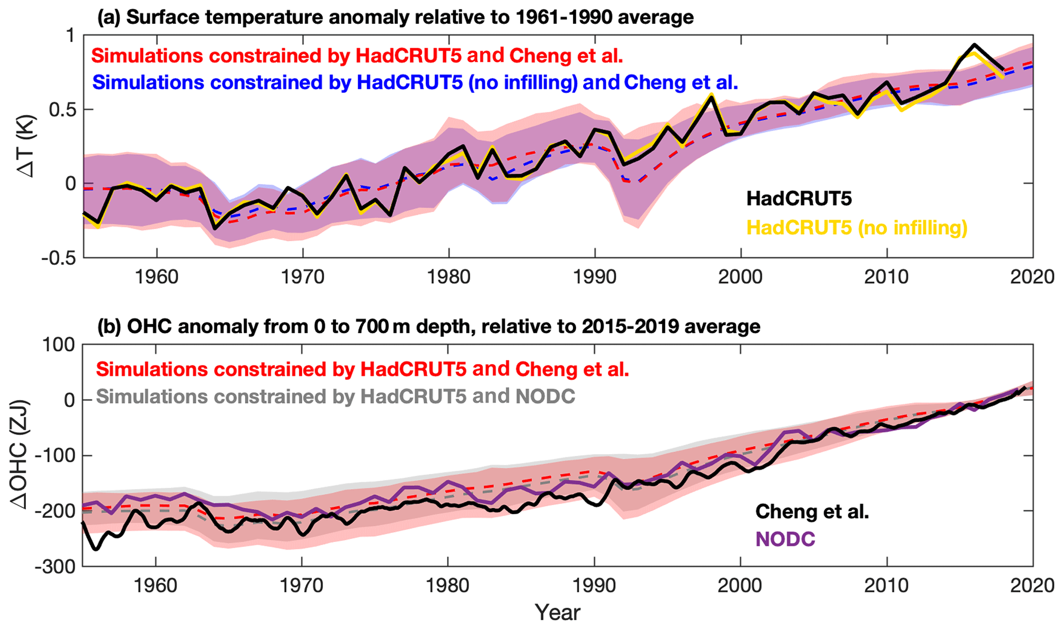
Figure 1 Surface temperature and ocean heat content anomalies from 1955 from datasets and dataset-constrained simulations. (a) Historic surface warming relative to the 1961–1990 average in the HadCRUT5 and HadCRUT5 (no infilling) surface temperature datasets (solid lines) and posterior ensemble simulations (dashed lines show ensemble medians, and shading shows 95 % ensemble ranges) constrained by each temperature dataset, along with the Cheng et al. ocean heat content dataset. (b) Ocean heat content (OHC) anomaly in the upper 700 m of the global ocean in the NODC and Cheng et al. datasets (solid lines) and posterior ensemble simulations (dashed lines show ensemble medians, and shading shows 95 % ensemble ranges) constrained by each OHC dataset along with the HadCRUT5 temperature dataset.

Many previous studies evaluating S from historical observational data and radiative forcing estimates (see Eq. 2) have either calculated a single constant climate sensitivity (see Annan, 2015; Annan and Hargreaves, 2020; Bodman and Jones, 2016; Lewis and Curry, 2014; Sherwood et al., 2020; Skeie et al., 2018; Otto et al., 2013; Nijsse et al., 2020) or have evaluated S for specific historic periods (e.g. Tokarska et al., 2020), acknowledging that the value for the specific historical period may not apply for all timescales into the future.

The assumption of a single constant S over time leads to uncertainties arising from model inadequacy (Annan, 2015), since climate sensitivity may not be constant with time or across different response timescales (e.g. Rugenstein et al., 2020; Rohling et al., 2012, 2018; Goodwin, 2018; Knutti et al., 2017; Senior and Mitchell, 2000; Proistosescu and Huybers, 2017). There is also the possibility that, at any given time or timescale, the climate feedback may be different for different sources of radiative forcing, such as well-mixed greenhouse gases and volcanic aerosols (e.g. Marvel et al., 2015).

The aim here is to perform Bayesian probabilistic evaluations of both S and transient climate response (TCR in K), using observational constraints on global surface temperature and ocean heat content anomalies to constrain a model framework that includes time-varying climate feedbacks (Eqs. 1 and 2). Our estimates of S and TCR are independent of simulated warming responses in complex climate models (in contrast to estimates utilizing complex model output via emergent constraints, e.g. Nijsse et al., 2020).

We utilize a numerical model that allows multiple climate feedbacks to individually respond to radiative forcing over different timescales (Goodwin, 2018), such that λ_eff varies over time (Eqs. 1 and 2). This study considers the instantaneous Planck feedback and two further timescales of climate feedback: a multiday feedback representing a selection of fast climate processes, such as water vapour and clouds, and a multi-decadal climate feedback representing slower processes, such as the surface warming pattern effect. Generating a prior model ensemble with varying fast and multi-decadal climate feedback strengths, we extract three posterior ensembles using a Bayesian comparison to observational reconstructions. Each posterior ensemble applies a different combination of historic reconstructions of global surface temperature anomaly (either HadCRUT5 or HadCRUT5 without statistical infilling of geographically absent data, hereafter HadCRUT5 (no infill); Morice et al., 2021; Fig. 1a) and a reconstruction of the ocean heat content anomaly (either Cheng et al., 2017, hereafter Cheng et al., or Levitus et al., 2012, hereafter NODC; Fig. 1b). All of our posterior ensembles are extracted using the additional constraints from HadSST4 (Kennedy et al., 2019) and the Global Carbon Budget (le Quéré et al., 2018) for sea surface temperature and ocean carbon uptake anomalies, respectively (see Supplement).

2 Model of surface warming from time-varying climate feedback

Equation (1) considers surface warming via a single effective climate feedback response to total radiative forcing, where the effective climate feedback represents an aggregated response to multiple climate feedbacks to multiple sources of radiative forcing. Here, surface warming is modelled as an extended energy balance response to i sources of radiative forcing by j climate feedbacks operating over different response timescales (Goodwin, 2018),

$$\begin{array}{}\text{(3)}& \mathrm{\Delta }T\left(t\right)=\left(\mathrm{1}-{\displaystyle \frac{N\left(t\right)}{R_{\text{total}}\left(t\right)}}\right)\sum _i\left[{\displaystyle \frac{R_i\left(t\right)}{{\mathit{\lambda }}_{\text{Planck}}+{\sum }_j{\mathit{\lambda }}_{i,j}\left(t\right)}}\right].\end{array}$$

The j combinations of climate feedbacks processes considered here are as follows.

1. λ_fast is the combined fast feedbacks operating over response timescales approximately linked to the residence timescale of water vapour in the atmosphere (van der Ent and Tuinenberg, 2017), including clouds, water vapour-lapse rate, snow and sea ice surface albedo.

2. λ_{multi-decadal} is the combined feedbacks operating over a multi-decadal timescale that may, for example, be linked to a surface warming pattern adjustment (e.g. Andrews et al., 2015).

Note that slow climate feedbacks with timescales longer than multi-decadal are not explored here, since the historical records of temperature and heat content changes do not extend long enough to offer a reliable constraint on processes acting on such long timescales. In addition, the snow and ice albedo feedback has a timescale longer than the atmospheric water vapour residence timescale but is included in λ_fast here as the snow and sea ice timescale responds significantly faster than multi-decadal timescales. The sign convention adopted has positive overall λ_eff, such that negative λ_fast and λ_{multi-decadal} are amplifying.

The Warming Acidification and Sea level Projector (WASP) model starts simulations at 1700 CE by default (e.g. Goodwin, 2018), with different sources of radiative forcing defined from some time after that date. While the observational constraints used in this study start in 1850 CE, the model state in 1850 is affected by radiative forcing received prior to that date. Therefore, this study imposes radiative forcing on the WASP model prior to 1850. The i sources of radiative forcing used in Eq. (3) are as follows:

1. atmospheric CO₂ forcing, calculated from CO₂ concentrations using $R_{{\mathrm{CO}}_{\mathrm{2}}}=a_{{\mathrm{CO}}_{\mathrm{2}}}\mathrm{\Delta }\ln {\mathrm{CO}}_{\mathrm{2}}$, following IPCC (2013);

2. combined forcing from other well-mixed greenhouse gases, R_WMGHG, including methane, nitrous oxides individually calculated from concentrations following Etminan et al. (2016) (see Supplement), and halocarbons following IPCC (2013);

3. combined direct and indirect anthropogenic aerosol forcing and linked annual aerosol emission rates (Myhre et al., 2013; Smith et al., 2018, see Supplement);

4. volcanic aerosol radiative forcing, calculated after 1850 from volcanic aerosol optical depth (AOD) using R_volcanic = −(19 ± 0.5)AOD (Gregory et al., 2016) and before 1850 from the global radiative forcing time series used in the Reduced Complexity Model Intercomparison Project (RCMIP) phase 1 (Nicholls et al., 2020), with identical relative uncertainty imposed both pre- and post-1850;

5. solar forcing;

6. internal variability in Earth's energy imbalance, imposed using AR1 noise with coefficients chosen to approximate the properties of monthly and yearly average noise from Trenberth et al. (2014).

The equations WASP uses to evolve climate feedback over time are presented in Goodwin (2018) and discussed here in the Supplement. Briefly, when radiative forcing from source i is not increasing in magnitude between times t−δt and t, $\mathrm{|}{R}_i\left(t\right)\mathrm{|}\le \mathrm{|}{R}_i(t-\mathit{\delta }t)\mathrm{|}$, the jth combination of climate feedback processes evolves according to the following equation (see Supplement):

$$\begin{array}{}\text{(4)}& \begin{array}{rl}{\mathit{\lambda }}_{i,j}\left(t\right)=& {\mathit{\lambda }}_{i,j}(t-\mathit{\delta }t)+\left({\mathit{\lambda }}_j^{\text{equil}}-{\mathit{\lambda }}_{i,j}(t-\mathit{\delta }t)\right)\\ & \cdot \left(\mathrm{1}-\exp \left({\displaystyle \frac{-\mathit{\delta }t}{{\mathit{\tau }}_j}}\right)\right).\end{array}\end{array}$$

However, when radiative forcing from source i is increasing in magnitude, $\mathrm{|}{R}_i(t+\mathit{\delta }t)\mathrm{|}>\mathrm{|}{R}_i\left(t\right)\mathrm{|}$, climate feedback λ_i,j evolves from t to t+δt according to the following equation (see Supplement):

$$\begin{array}{}\text{(5)}& \begin{array}{rl}& {\mathit{\lambda }}_{i,j}\left(t\right)=\left|{\displaystyle \frac{R_i(t-\mathit{\delta }t)}{R_i\left(t\right)}}\right|\left({\mathit{\lambda }}_{i,j}\right(t-\mathit{\delta }t)+\left({\mathit{\lambda }}_j^{\text{equil}}-{\mathit{\lambda }}_{i,j}(t-\mathit{\delta }t)\right)\\ & \cdot \left(\mathrm{1}-\exp \left({\displaystyle \frac{-\mathit{\delta }t}{{\mathit{\tau }}_j}}\right)\right)).\end{array}\end{array}$$

Thus, from Eqs. (3)–(5), any additional radiative forcing acts instantaneously at the Planck feedback in the first time step it is applied and then evolves over the e-folding response timescales τ_j towards the equilibrium climate feedback: λ_equilibrium = ${\mathit{\lambda }}_{\text{Planck}}+{\mathit{\lambda }}_{\text{fast}}^{\text{equil}}+{\mathit{\lambda }}_{\text{multi-decadal}}^{\text{equil}}$. Figure S7 in the Supplement shows how climate feedback evolves over time in response to an idealized radiative forcing using Eqs. (4) and (5). Since Eq. (5) is applied separately for each of the i sources of radiative forcing, the framework used here allows different values of climate feedback at any point in time for each source of radiative forcing.

This model of climate feedbacks responding to imposed radiative forcing over multiple response timescales, Eqs. (3)–(5), produces a time-evolving effective climate feedback, Eq. (1), and time-evolving climate sensitivity, Eq. (2), in response to a prescribed forcing scenario. Here, the transient climate response, TCR, is calculated as the 20-year average warming centred at the year of CO₂ doubling for a scenario with a 1 % yr⁻¹ rise in CO₂ and no other forcing (hereafter, the 1pctCO₂ scenario).

Figure 2 Prior and posterior probability densities for climate feedback terms: (a) the Planck climate feedback, (b) fast climate feedback, and (c) multi-decadal climate feedback. Shown are the prior distributions (thick black lines) and posterior distributions when constrained by different dataset combinations (dotted blue, red, and grey lines). Panel (d) shows a scatter plot of fast climate feedback and multi-decadal climate feedback values in the posterior ensemble constrained by the HadCRUT5 and Cheng et al. datasets.

3 Generation of the prior and posterior ensembles

We generate probabilistic prior and posterior model ensembles with varied model input parameters using Bayes' theorem. The joint posterior probability that the climate system parameters X have a specific set of values X^′ given background information I and observations of the climate system {obs}, $\text{prob}(X=X^{\prime }\mathrm{|}\mathit{\{}\text{obs}\mathit{\}},I)$, is expressed using Bayes' theorem,

$$\begin{array}{}\text{(6)}& \begin{array}{rl}& \text{prob}(X=X^{\prime }\mathrm{|}\mathit{\{}\text{obs}\mathit{\}},I)\propto \text{prob}\left(\mathit{\right\{}\text{obs}\mathit{\}}\mathrm{|}X=X^{\prime },I)\\ & \cdot \text{prob}(X=X^{\prime }\mathrm{|}I),\end{array}\end{array}$$

where

1. $\text{prob}(X=X^{\prime }\mathrm{|}I)$ is the joint prior probability that $X=X^{\prime }$ for climate system parameter values (Table S1 in the Supplement; solid lines in Fig. 2 for λ_Planck, ${\mathit{\lambda }}_{\text{fast}}^{\text{equil}}$, and ${\mathit{\lambda }}_{\text{multi-decadal}}^{\text{equil}}$);

2. $\text{prob}\left(\mathit{\right\{}\text{obs}\mathit{\}}\mathrm{|}X=X^{\prime },I)$ is known as the likelihood function and expresses the probability of obtaining the observations in {obs} for the given joint parameter values $X=X^{\prime }$ and background information I. Here, this is estimated from where the simulated model observables for $X=X^{\prime }$ and I lie on the probability distributions for the real observables (Table S2 in the Supplement).

Here, we use large ensemble simulations of the WASP model (Goodwin, 2016), adopting the updated version of Goodwin (2018) with explicitly time-evolving climate feedbacks (Eqs. 3–5; see Supplement). This version of WASP does not contain a single parameter for S or λ_eff at time t; see Eqs. (1) and (2). Instead, the values of S and λ_eff emerge over time in the model in response to the forcing scenario from a combination of multiple prescribed climate system parameters (Eqs. 3–5). The WASP model contains a five-box representation of ocean heat and carbon uptake, with an ocean circulation that is varied between ensemble members but remains constant in time within each ensemble member (Table S1).

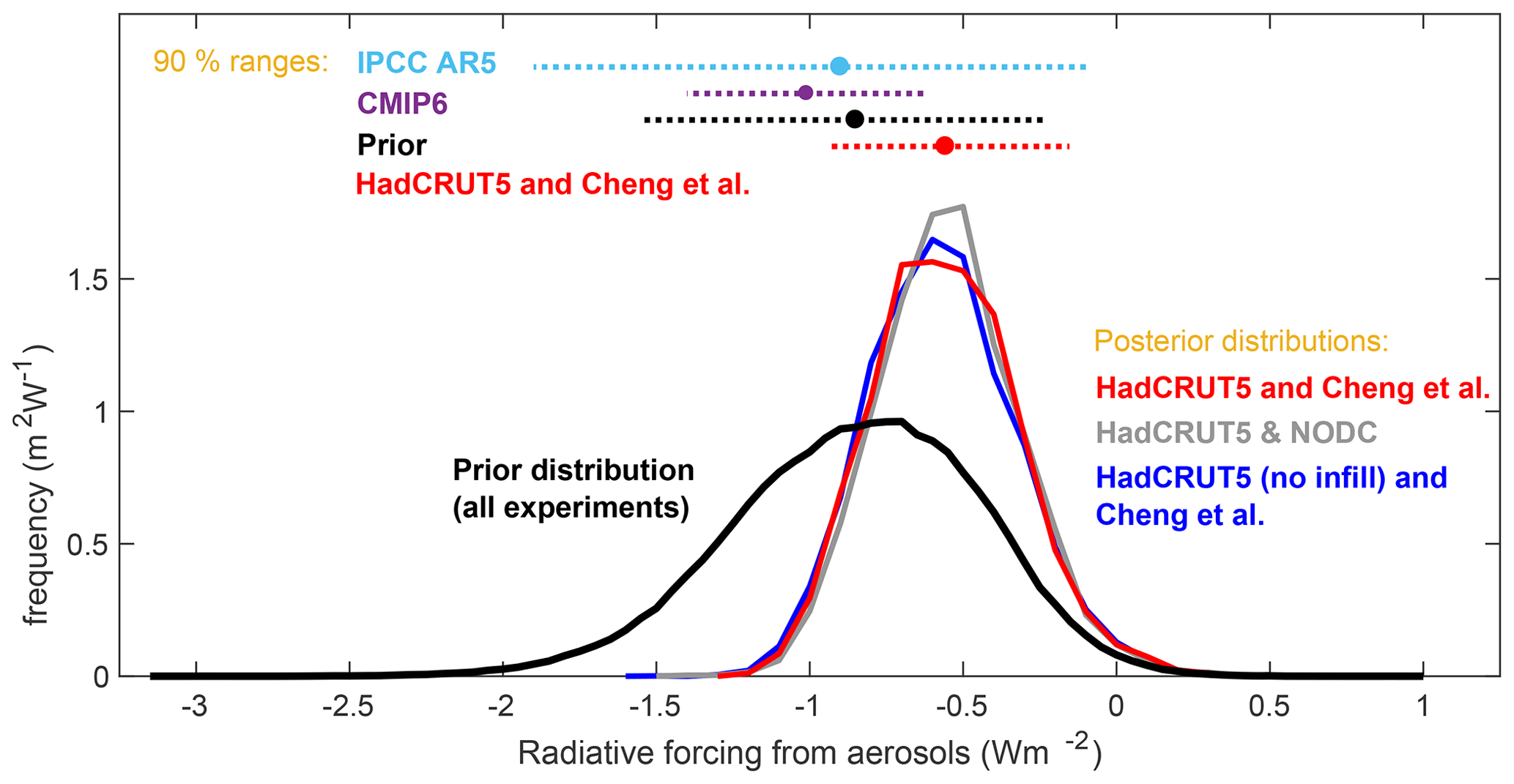
Figure 3 Recent radiative forcing from aerosols in model ensembles and estimates. Solid lines are frequency distributions from the prior model ensembles (black) and posterior model ensembles constrained by different combinations of observational datasets (red, grey, and blue). Also shown are 90 % ranges (dotted lines) and best estimates (circles) from IPCC AR5 (IPCC, 2013: light blue), an ensemble of 17 CMIP6 models analysed by Smith et al. (2020) (purple), and the prior and HadCRUT5 and Cheng et al. posterior model ensembles. For model ensembles the best estimate is calculated from the model ensemble mean. The 90 % range represents the 5th to 95th percentile in the prior and HadCRUT5 and Cheng et al. model ensembles and represents the mean ± 1.645 standard deviations for the CMIP6 model ensemble. All distributions are for the year 2014, except the IPCC AR5 estimate, which is for the year 2011.

We form a prior model ensemble where a total of 25 model input parameters independently varied between simulations (Table S1) to represent the prior climate system parameter distribution X; see Eq. (6). Five of the input parameters within X describe how climate feedback responds to an imposed radiative forcing (λ_Planck, ${\mathit{\lambda }}_{\text{fast}}^{\text{equil}}$, ${\mathit{\lambda }}_{\text{multi-decadal}}^{\text{equil}}$, τ_Fast, and τ_Slow) with a sixth input parameter (the radiative forcing coefficient for CO₂) converting this climate feedback to climate sensitivity (Table S1, Eq. 2). The λ_Planck parameter is randomly varied from normal distribution (Fig. 2a, solid black line), while the ${\mathit{\lambda }}_{\text{fast}}^{\text{equil}}$ and ${\mathit{\lambda }}_{\text{multi-decadal}}^{\text{equil}}$ parameters are randomly varied from uniform distributions (Fig. 2b and c, solid black lines), reflecting the degree of assumed prior knowledge of their values (Supplement).

A further 13 of the 25 model input parameters that varied within X relate to uncertainty in historic radiative forcing (Table S1). The WASP model is historically forced until 2014 and follows ssp585 thereafter (O'Neill et al., 2016) with atmospheric concentrations of greenhouse gases, direct and indirect radiative forcing from anthropogenic aerosols, radiative forcing from volcanic aerosols, and solar forcing (see Supplement). The radiative forcing from each component (aside from solar forcing) is varied between simulations in the prior ensemble (Table S1) to approximate historic uncertainty (Myhre et al., 2013; Etminan et al., 2016; Smith et al., 2018; Gregory et al., 2016).

Normal input distributions (Table S1) are used to represent historic uncertainty in the radiative forcing sensitivity to greenhouse gas concentrations (Myhre et al., 2013; Etminan et al., 2016), the direct radiative forcing sensitivity to anthropogenic aerosol emissions for six separate aerosol types (Myhre et al., 2013), and the radiative forcing sensitivity to volcanic aerosol optical depth (Gregory et al., 2016). However, a skew normal input distribution is used to represent historic uncertainty in the indirect radiative forcing from anthropogenic aerosols (Table S1) since there is a long tail of possibly strongly negative radiative forcing from this effect (IPCC, 2013). The input distributions of direct and indirect aerosol radiative forcing coefficients together produce a broad and skewed prior distribution of total recent radiative forcing from aerosols (Fig. 3, solid and dotted black lines, shown for year 2014) with a similar mean to the best estimate of recent aerosol radiative forcing from IPCC (2013) Assessment Report 5 (Fig. 3, compare black lines to light blue lines, with the IPCC AR5 estimate shown for year 2011).

We generate three prior ensembles, containing from 2.1 × 10⁹ to 4.6 × 10⁹ ensemble members. In each prior ensemble, the 25 input parameters independently varied such that the relative frequency distributions of each input parameter are set to the assumed prior probability distribution, $\text{prob}(X=X^{\prime }\mathrm{|}I)$ in Eq. (6) (Table S1; Fig. 2 solid lines for λ_Planck, ${\mathit{\lambda }}_{\text{fast}}^{\text{equil}}$, and ${\mathit{\lambda }}_{\text{multi-decadal}}^{\text{equil}}$). Observational tests from three combinations of historic datasets are then used to form a likelihood function and extract a subset of the prior ensemble simulations into the posterior ensembles (Table S2).

There are n=12 observational constraints within {obs} (Table S2). The probability of obtaining the kth observational constraint given $X=X^{\prime }$ and I is calculated assuming Gaussian uncertainty in the observable (e.g. Annan and Hargreaves, 2020),

$$\begin{array}{}\text{(7)}& \text{prob}\left(\mathit{\{}\text{obs}{\mathit{\}}}_{\mathrm{k}}\mathrm{|}X=X^{\prime },I\right)\propto e^{\frac{-({\mathit{\mu }}_{\mathrm{k}}-x_{\mathrm{k}}{)}^{\mathrm{2}}}{\mathrm{2}{\mathit{\sigma }}_{\mathrm{k}}^{\mathrm{2}}}},\end{array}$$

where μ_k and σ_k are the observational mean and standard deviation uncertainty of observable k (Table S2), and x_k is the simulated value of the observable for $X=X^{\prime }$ and I. To calculate the overall probability of obtaining all n observational constraints within obs given $X=X^{\prime }$ and I, we multiply the probabilities for all {obs}_k,

$$\begin{array}{}\text{(8)}& \text{prob}\left(\mathit{\left\{}\text{obs}\mathit{\right\}}\mathrm{|}X=X^{\prime },I\right)=\prod _{k=\mathrm{1}}^n\text{prob}\left(\mathit{\{}\text{obs}{\mathit{\}}}_{\mathrm{k}}\mathrm{|}X=X^{\prime },I\right).\end{array}$$

Three different ensembles are generated using different combinations of surface temperature (HadCRUT5 and HadCRUT5 (no infilling): Fig. 1a) and heat content (Cheng et al. and NODC: Fig. 1b) datasets to construct the likelihood function that acts as a constraint on the posterior (Eq. 6). These model ensembles are termed HadCRUT5 and Cheng et al., HadCRUT5 and NODC, and HadCRUT5 (no infilling) and Cheng et al. (Table S2). The preferred combination of observational datasets is HadCRUT5 and Cheng et al., as these represent the most up-to-date methodologies for their respective temperature (Morice et al., 2021) and heat content (Cheng et al., 2017) reconstructions. The other dataset combinations are included to assess the sensitivity of our method to different heat content datasets (HadCRUT5 and NODC) and the sensitivity of our findings to the statistical infilling of missing data (HadCRUT5 (no infill) and Cheng et al.). It is noted that most other temperature datasets now reconstruct similar historic global mean temperature anomalies to HadCRUT5 (e.g. see Morice et al. 2021).

For each of the three posterior ensembles, corresponding to different dataset combinations, the probability of a prior simulation being included within the posterior ensemble is proportional to $\text{prob}\left(\mathit{\right\{}\text{obs}\mathit{\}}\mathrm{|}X=X^{\prime },I)$; see Eq. (8). A simulation is accepted into the posterior ensemble if the value of $\text{prob}\left(\mathit{\right\{}\text{obs}\mathit{\}}\mathrm{|}X=X^{\prime },I)$, assessed using Eq. (8), is greater than a number randomly drawn between 0 and some number greater than or equal to the maximum value of $\text{prob}\left(\mathit{\left\{}\text{obs}\mathit{\right\}}\mathrm{|}X=X^{\prime },I\right)$ achieved in that prior ensemble.

We adopt a normal prior distribution for λ_Planck, informed by Earth's global mean surface temperature (Jones and Harpham, 2013) and radiation budget (Trenberth et al., 2014) (Fig. 2a, solid black line). We adopt uniform prior distributions of ${\mathit{\lambda }}_{\text{fast}}^{\text{equil}}$ and ${\mathit{\lambda }}_{\text{multi-decadal}}^{\text{equil}}$ (Fig. 2b and c solid black lines), thus assuming that any value within the boundaries is equally likely before we consider the observations, {obs} (Eq. 6). Our boundaries for the uniform distributions of ${\mathit{\lambda }}_{\text{fast}}^{\text{equil}}$ and ${\mathit{\lambda }}_{\text{multi-decadal}}^{\text{equil}}$ are set wide enough such that the posterior distributions are not significantly affected by the boundaries (Fig. 2, red and blue) but are narrow enough such that the problem is computationally tractable. The distribution for ${\mathit{\lambda }}_{\text{multi-decadal}}^{\text{equil}}$ is centred at 0, such that no prior assumption is made as to whether multi-decadal feedbacks will amplify or dampen future warming (Fig. 2).

4 Results

The three prior and posterior ensembles generated clearly range in size: a total of 1764 simulations are accepted into the HadCRUT5 and Cheng et al. posterior ensemble from an initial prior ensemble of 4.6 × 10⁹ simulations, a total of 2997 simulations are accepted into the HADCRUT5 and NODC posterior ensemble from an initial prior ensemble of 2.7 × 10⁹ simulations, and 9190 simulations are accepted into the HadCRUT5 (no infill) and Cheng et al. posterior ensemble from an initial prior ensemble of 2.1 × 10⁹ simulations. A smaller fraction of the prior simulations are accepted into the posterior ensembles that use likelihood function terms, $\text{prob}\left(\mathit{\right\{}\text{obs}{\mathit{\}}}_{\mathrm{k}}\mathrm{|}X=X^{\prime },I)$ in Eq. (7), with smaller observational uncertainty, σ_k (Table S2).

The posterior distributions of climate feedback terms are similar for both ensembles constrained by the HadCRUT5 dataset (HadCRUT5 and Cheng et al., and HadCRUT5 and NODC), revealing that the Planck feedback, fast feedback, and multi-decadal feedback strengths are insensitive to the choice of ocean heat content dataset used within the likelihood function (Fig. 2a–c compare red and grey). The Planck feedback has posterior distributions in the range λ_Planck = 3.3 ± 0.1 $\mathrm{W}{\mathrm{m}}^{-\mathrm{2}}{\mathrm{K}}^{-\mathrm{1}}$ for both ensembles (mean ± standard deviation: Fig. 2a, red and grey).

A strong compensatory link between fast and multi-decadal feedback strengths emerges in the posterior ensembles, with the HadCRUT5 and Cheng et al. ensemble revealing a best fit relationship of ${\mathit{\lambda }}_{\text{fast}}^{\text{equil}}=-\mathrm{1.59}{\mathit{\lambda }}_{\text{multi-decadal}}^{\text{equil}}-\mathrm{2.51}$, with R² = 0.92 (Fig. 2d). The posterior distributions for fast and multi-decadal climate feedback strengths are bimodal in the HadCRUT5 and Cheng et al. and HadCRUT5 and NODC ensembles (Fig. 2b and c, red and grey), corresponding to one observation-consistent region with weaker amplifying fast feedback (${\mathit{\lambda }}_{\text{fast}}^{\text{equil}}$ ∼ −0.6 W m⁻²) and strong amplifying multi-decadal feedback (${\mathit{\lambda }}_{\text{multi-decadal}}^{\text{equil}}$ ∼ −1.7 W m⁻²) and another observation-consistent region with very strong amplifying fast feedback (${\mathit{\lambda }}_{\text{fast}}^{\text{equil}}$ ∼ −2.2 W m⁻²) and damping multi-decadal feedback (${\mathit{\lambda }}_{\text{multi-decadal}}^{\text{equil}}$ ∼ +1 W m⁻²) (Fig. 2d, shown for the HadCRUT5 and Cheng et al. ensemble), noting that the sign convention used implies amplifying feedback from negative λ. This bimodality, with an unfavoured region around ${\mathit{\lambda }}_{\text{multi-decadal}}^{\text{equil}}\sim \mathrm{0}$ (Fig. 2), is consistent with effective climate feedback changing over the historic period (e.g. Gregory et al., 2019), since ${\mathit{\lambda }}_{\text{multi-decadal}}^{\text{equil}}=\mathrm{0}$ would correspond with a constant value of λ_eff over the entire historic period. The bimodality in the ${\mathit{\lambda }}_{\text{fast}}^{\text{equil}}$ and ${\mathit{\lambda }}_{\text{multi-decadal}}^{\text{equil}}$ posterior distributions is not seen in the ensemble constrained by the temperature reconstruction without statistical infilling (HadCRUT5 (no infill) and Cheng et al.), which instead has broader single-peak distributions (Fig. 2b and c blue).

Figure 4 Climate sensitivity (S) from 10- to 140-year response timescales following a 4×CO₂ forcing scenario constrained by different combinations of observational reconstructions. Solid lines show the median, dashed lines and dark shading show the 66 % range (17th to 83rd percentiles), and dotted lines and light shading show the 95 % range (2.5th to 97.5th percentiles). Panels (a), (b), and (c) show results from posterior model ensembles constrained by different dataset combinations, where red lines on panels (b) and (c) give a comparison to HadCRUT5 and Cheng et al.

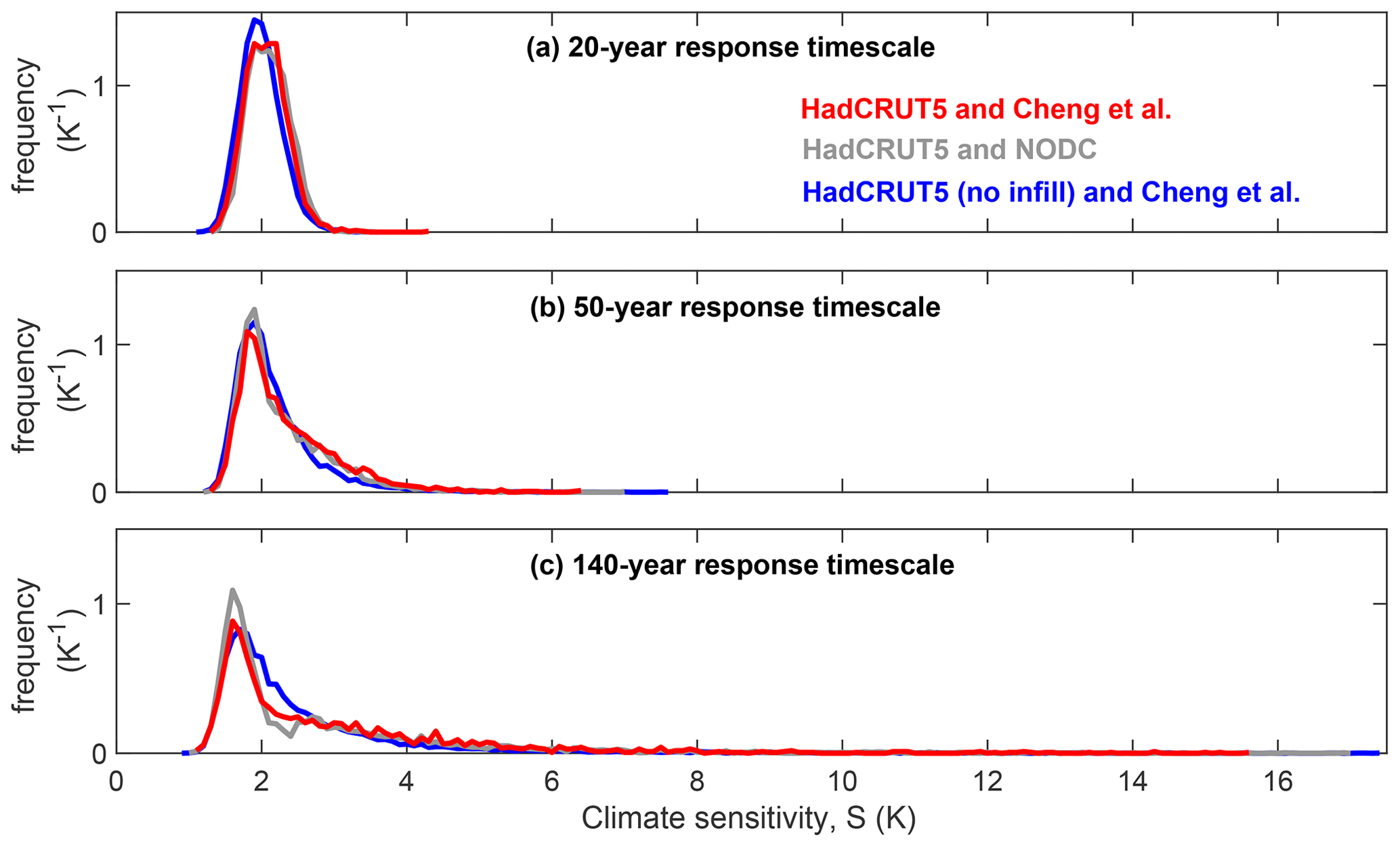
Figure 5 Probabilistic estimates of climate sensitivity (S) for different combinations of observational constraints over (a) a 20-year response timescale, (b) a 50-year response timescale, and (c) a 140-year response timescale.

4.1 The climate sensitivity and transient climate response

S is analysed by forcing the four posterior ensembles with an instantaneous step-function quadrupling of atmospheric CO₂ (hereafter, the 4×CO₂ scenario) and applying Eq. (2) with 11-year averages. The value of S changes over time (Figs. 4 and 5) as the fast and multi-decadal climate feedbacks evolve in response to the imposed radiative forcing (Eqs. 3–5).

Table 1 Climate sensitivity (S, K) and transient climate response (TCR, K) best estimate (median) and ranges (where 66 % confidence interval represents the 17th to 83rd percentile range, 90 % confidence interval represents 5th to 95th percentile range, and 95 % confidence interval represents 2.5th to 97.5th percentile range) under different observational constraints for surface warming and heat uptake. All ensembles use the standard prior distributions (Table S1) except “HadCRUT5 and Cheng et al. (with alternative multi-decadal climate feedback prior)”, which uses the prior for λ_{multi-decadal} from Sherwood et al. (2020) (Fig. 8c, purple) and standard priors for all other terms.

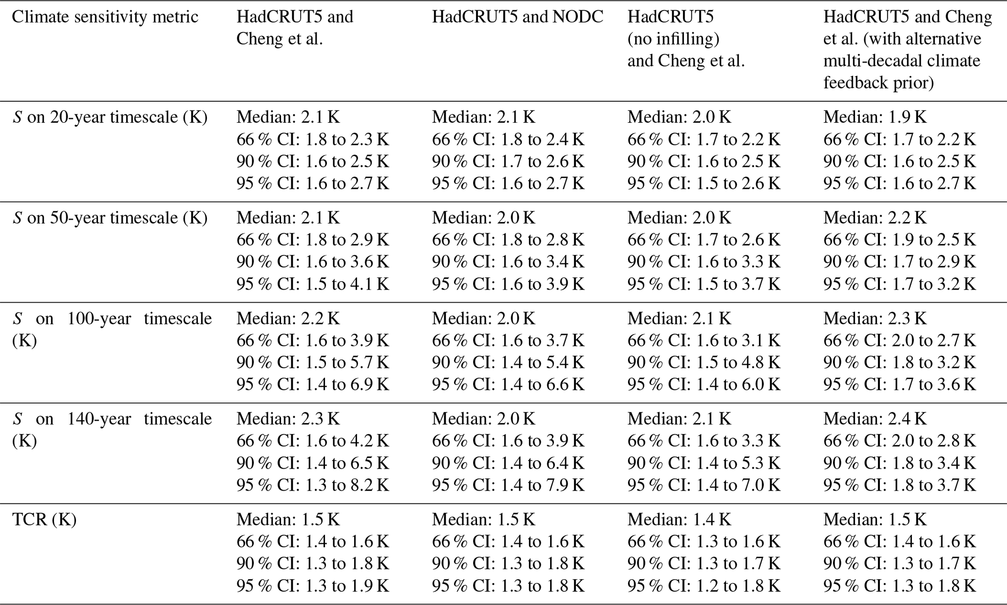
For each combination of datasets used, S is best constrained from the historic observational reconstructions on a 20-year timescale (Figs. 4 and 5a, Table 1). These 20-year response timescale S estimates are also similar between different dataset combinations: varying from 2.1 ^∘C (1.6 to 2.5 ^∘C at 90 % range from 5th to 95th percentiles) for the HadCRUT5 and Cheng et al. dataset combination to 2.1 ^∘C (1.7 to 2.6 ^∘C) for the HadCRUT5 and NODC dataset combination.

The distributions see a general increase in S out to 50-,100-, and 140-year timescales, with greater uncertainty (Figs. 4 and 5; Table 1) due to the uncertainty in how multi-decadal climate feedback will evolve (Fig. 2). The TCR is analysed by forcing our posterior ensembles with a 1pctCO₂ scenario and recording the surface warming for each ensemble member for the 20-year average centred on the year in which CO₂ reaches twice its initial value (Fig. 6; Table 1). Our analysis reveals a TCR of 1.5 (1.3 to 1.8 at 90 % range) ^∘C when constrained by the HadCRUT5 temperature reconstruction with either ocean heat content dataset (Table 1).

4.2 Variation in the posterior model ensembles

The observational records provide constraints on the parameters of the posterior ensembles that manifest not only as posterior distributions for these parameters but also as relationships between them, as well as between model parameters and key model outputs of interest (such as S(t)). While the correlation structure of the 25 parameters' joint posterior distribution is generally quite complex, some key structures emerge that indicate how S and TCR uncertainties might be reduced. This method of analysing variation and simplifying the degrees of freedom of variation in large data-constrained efficient model ensembles may ultimately help explore parameter space in more complex Earth system models.

Figure 6 Transient climate response (TCR) for combinations of temperature and heat content datasets, evaluated from 1pctCO₂ scenario using the 20-year average warming centred on the moment of CO₂ doubling.

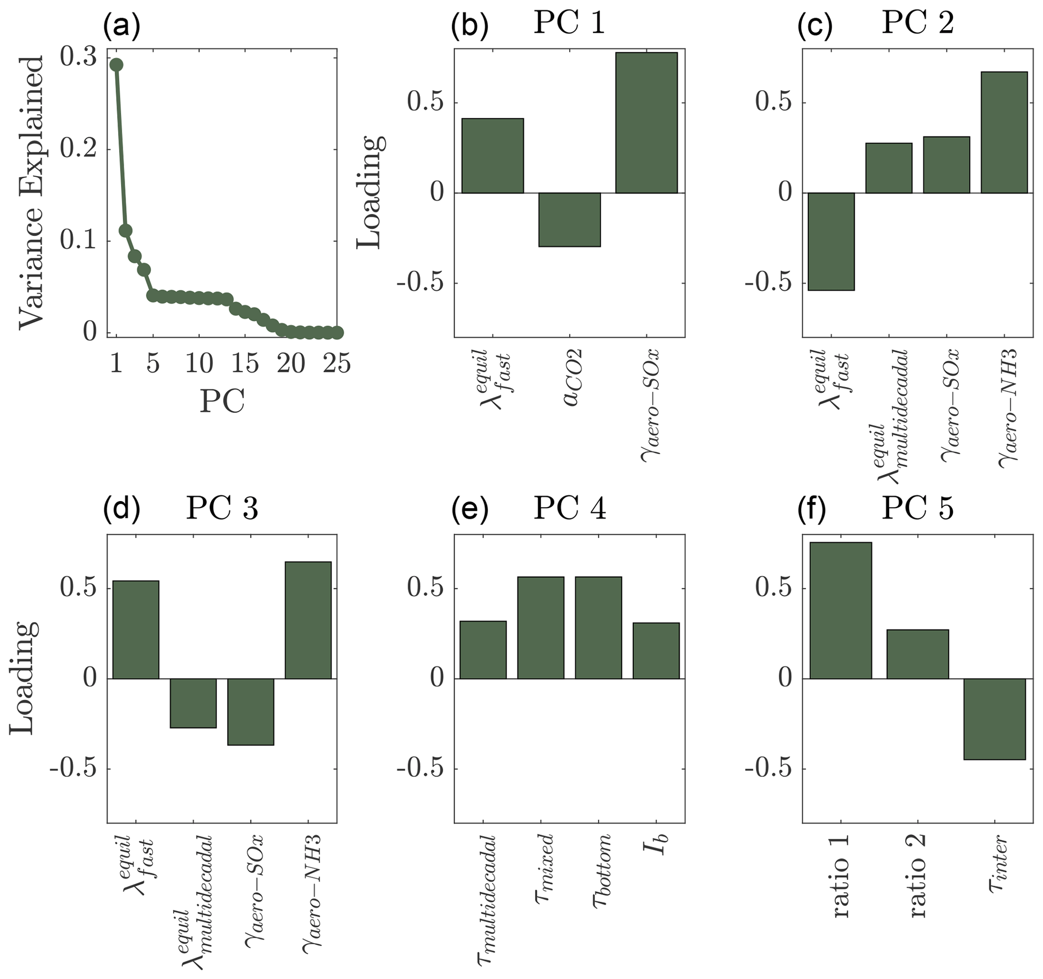
Figure 7 Principal component analysis of the posterior model ensembles. Shown is a scree plot of principal component (PC) vs. variance explained and PCs 1–5, simplified by showing only the model parameters with loading greater than 0.25 in magnitude. All 25 varied model parameters are fully defined in Table S1. Briefly, a_CO2 is the CO₂ radiative forcing coefficient; γ_aero-XX terms reflect the sensitivity of radiative forcing to aerosol type XX; τ_{multi-decadal} is the timescale for multi-decadal feedback; τ_mixed, τ_inter, and τ_bottom are the ocean ventilation timescales for the ocean surface mixed layer, intermediate water, and bottom water, respectively; I_b is the buffered carbon inventory of the air–sea system; ratio 1 is the ratio of warming for global surface temperatures relative to global sea surface temperatures at equilibrium; and ratio 2 is the ratio of warming for the whole ocean temperatures relative to sea surface temperatures at equilibrium.

4.2.1 Correlations of model parameters and outputs

We assemble the three observationally consistent ensembles into a single meta-ensemble, where each model realization is weighted inversely to the number of members in its individual ensemble such that each of the three observational combinations is weighed equally (henceforth all analyses in this section are weighted, i.e. weighted correlations, weighted principal component analysis, and weighted stepwise regression). We then first examine the correlations between individual model parameters. We find three strongly correlated groups of model parameters (Fig. S1 in the Supplement). First, the ${\mathit{\lambda }}_{\text{multi-decadal}}^{\text{equil}}$ and ${\mathit{\lambda }}_{\text{fast}}^{\text{equil}}$ feedback parameters are strongly compensating (ρ = −0.95) and the λ_Planck feedback is also fairly well correlated with these (ρ=0.49 and −0.56, respectively). Second, ratio 1 (the ratio of global near-surface warming to global sea surface warming at equilibrium) and ratio 2 (the ratio of global whole-ocean warming to global sea surface warming at equilibrium) parameters strongly compensate (ρ = −0.85), indicating the ratio of near-surface warming to global whole-ocean warming is tightly constrained by these datasets. Finally, all of the greenhouse gas and aerosol sensitivities are well correlated, with |ρ|≥0.4 (except for the aerosol indirect effect). None of these are surprising as they reflect the primary constraints of the observations, i.e. ocean, near-surface warming, and radiative forcing histories, but the former does indicate that a better-constrained fast feedback parameter would directly reduce uncertainty on multi-decadal feedbacks and thereby S on multi-decadal and centennial timescales. Model outputs are in general correlated in expected fashions with each other and with model parameters. TCR is well correlated with S on all timescales (20, 50, 100, and 140 years), and S on timescales greater than 20 years is also well correlated, whereas S₂₀ is only weakly correlated with these as it is controlled by other feedback parameters. We therefore focus on TCR, S₂₀, and S₁₀₀ hereafter. S and TCR are, as expected, very strongly correlated with the feedback parameters and also appreciably correlated with greenhouse gas and aerosol sensitivity parameters but are weakly correlated with most other model parameters.

4.2.2 Principal components

Correlations between model parameters' posteriors imply that the dimensionality of the parameter space can be reduced and that the observational constraints collapse the posterior solution into a parameter space with fewer degrees of freedom. Principal component analysis (PCA; Jolliffe, 1986; note that we do not describe the method here as it is well described in many textbooks such as Jolliffe, 1986) is a straightforward, ubiquitous means to identify these degrees of freedom and is justifiable here in the absence of strongly non-linear model equations and given the Gaussian or near-Gaussian likelihoods and priors.

We perform a PCA on the model parameters' joint posterior; the results are presented in Fig. 7. In the scree plot (Fig. 7a), there is an obvious break point at the fifth principal component (PC), indicating the first five PCs are interpretable and the remaining are unstructured variations (Cattell, 1966). These PCs are shown in Fig. 7b–f, with loadings of only the parameters with the absolute value of the loading > 0.25 shown (full PCs are shown in Figs. S2–S6 in the Supplement for completeness). The first three of these PCs are dominated by the fast and multi-decadal feedbacks and the sensitivity of radiative forcing to CO₂ and two aerosols (SO_x and NH₃) (Fig. 7b–d). The fourth and fifth PC are dominated by oceanic factors (Fig. 7e and f): the timescales of the multi-decadal feedback and the ventilation of different ocean fractions, the buffered carbon inventory, and the warming ratios of near-surface to sea surface and sea surface to whole-ocean warming. Altogether, these PCA results suggest that the observational constraints used herein collapse the 25 model parameters around a five-dimensional subspace and that these five dimensions reflect the balance between the effects of climate feedbacks, greenhouse gases, and aerosols on atmospheric and oceanic warming, as well as the structure of the large-scale ocean circulation.

Note also there are numerous ways to quantify the number of interpretable or meaningful PCs resulting from a PCA (Jackson, 1993); the first five PCs we focus on here explain 60 % of the total variance in the dataset, but the decisive break in the scree plot (Fig. 7a) indicates strong evidence that these PCs are qualitatively different to the remaining PCs (6–25). We interpret the remaining variance in the data as reflective of the large amount of parametric uncertainty left in these models beyond what the observations herein can constrain, attesting to the importance of large ensemble simulations as employed here for quantifying uncertainty in S and TCR.

4.2.3 Stepwise regression

It is also of interest to what extent the model outputs are directly predictable from or explicable by the individual model parameters and/or PCs. Given the roughly Gaussian and linear model equations, multilinear regression is a suitable approach to identifying these links. Stepwise regression (Draper and Smith, 1981) in particular follows an automatic procedure of including and removing explanatory variables from the model fit to identify an optimal combination. We perform stepwise regression to predict the model outputs from the model parameters, (de)selecting explanatory variables using the Bayesian information criterion (Schwarz, 1978) and also including interactions between model parameters (i.e. their products).

We find S₁₀₀ to be a significant function of PC1–5 and their interactions, with an R²=0.50. While this is not an especially good fit, it is 83 % of the variance in the model parameters explained by these PCs; i.e. almost all of the model parameter variance these PCs explain directly translates to explained variance in S₁₀₀. In combination with the PCA results, this suggests the observations used here collapse the model parameters around five degrees of freedom and that S₁₀₀ is proportional to these degrees of freedom and their interactions, with the remaining variance in S₁₀₀ due to the remaining variance in the model parameters. This implies that the observational constraints used here directly constrain S₁₀₀ in our modelling approach, with very little information lost through constraining model parameters. In contrast, S₂₀ and TCR are more poorly predicted from these PCs (R²=0.37 and 0.19, respectively).

We also performed stepwise regression of model outputs against the 25 model parameters. We found S₁₀₀ to be a significant function of only nine model parameters (the three feedback parameters; the multi-decadal feedback timescale; and the sensitivities to CO₂, SO_x, aerosol indirect forcing, volatile organic compounds (VOCs), and N₂O), but it was very well predicted by these parameters (R²=0.86). S₂₀ was even better predicted (R²=0.96) by a similar suite of parameters (exchanging sensitivities to aerosol indirect forcing, VOCs, and N₂O with sensitivity to CH₄). This implies both that S is not strongly dependent on the other parameters in the model used here and also that there is a large amount of variation in S that can be reduced by better constraining these parameters. In contrast, TCR is sensitive to more model parameters (15) but is also similarly predictable from these (R²=0.95).

4.3 Choice of priors and the sensitivity of results

The prior distributions for climate feedback terms adopted here (Fig. 2a–c, black; Table S1) will impact the posterior distributions for climate feedback terms, TCR, S₂₀, S₅₀, S₁₀₀, and S₁₄₀ (Table 1). However the question remains as to how much they will be impacted. Our prior distribution for ${\mathit{\lambda }}_{\text{Planck}}^{\text{equil}}$ is chosen as normal with a mean of 3.3 $\mathrm{W}{\mathrm{m}}^{-\mathrm{2}}{\mathrm{K}}^{-\mathrm{1}}$ and standard deviation of ± 0.2 $\mathrm{W}{\mathrm{m}}^{-\mathrm{2}}{\mathrm{K}}^{-\mathrm{1}}$ since we have high confidence in the value from observational evidence (Jones and Harpham, 2013; Trenberth et al., 2014). However, the prior distributions for ${\mathit{\lambda }}_{\text{fast}}^{\text{equil}}$ and ${\mathit{\lambda }}_{\text{multi-decadal}}^{\text{equil}}$ are uniform over broad ranges (Fig. 2b and c, black) to reflect our initial ignorance as to their values (before applying observational constraints, Table S2). Both prior distributions for ${\mathit{\lambda }}_{\text{fast}}^{\text{equil}}$ and ${\mathit{\lambda }}_{\text{multi-decadal}}^{\text{equil}}$ have minimum values of −3.0 $\mathrm{W}{\mathrm{m}}^{-\mathrm{2}}{\mathrm{K}}^{-\mathrm{1}}$, chosen to be just less in magnitude than (and opposite in sign to) the mean in the prior for ${\mathit{\lambda }}_{\text{Planck}}^{\text{equil}}$ because we know that the total feedback must be positive on any timescale. The maximum value for ${\mathit{\lambda }}_{\text{multi-decadal}}^{\text{equil}}$ is chosen to be +3.0 $\mathrm{W}{\mathrm{m}}^{-\mathrm{2}}{\mathrm{K}}^{-\mathrm{1}}$ so that the prior distribution for multi-decadal feedbacks is symmetric around 0 and so that multi-decadal feedbacks have an equal prior likelihood of amplifying or damping surface warming. The range of ${\mathit{\lambda }}_{\text{fast}}^{\text{equil}}$ is chosen to have maximum of +1.0 $\mathrm{W}{\mathrm{m}}^{-\mathrm{2}}{\mathrm{K}}^{-\mathrm{1}}$ to maximize computational efficiency, as this is higher than the maximum values found in the posterior ensembles (Fig. 2c, dotted lines), and thus there is no need to extend the distribution further.

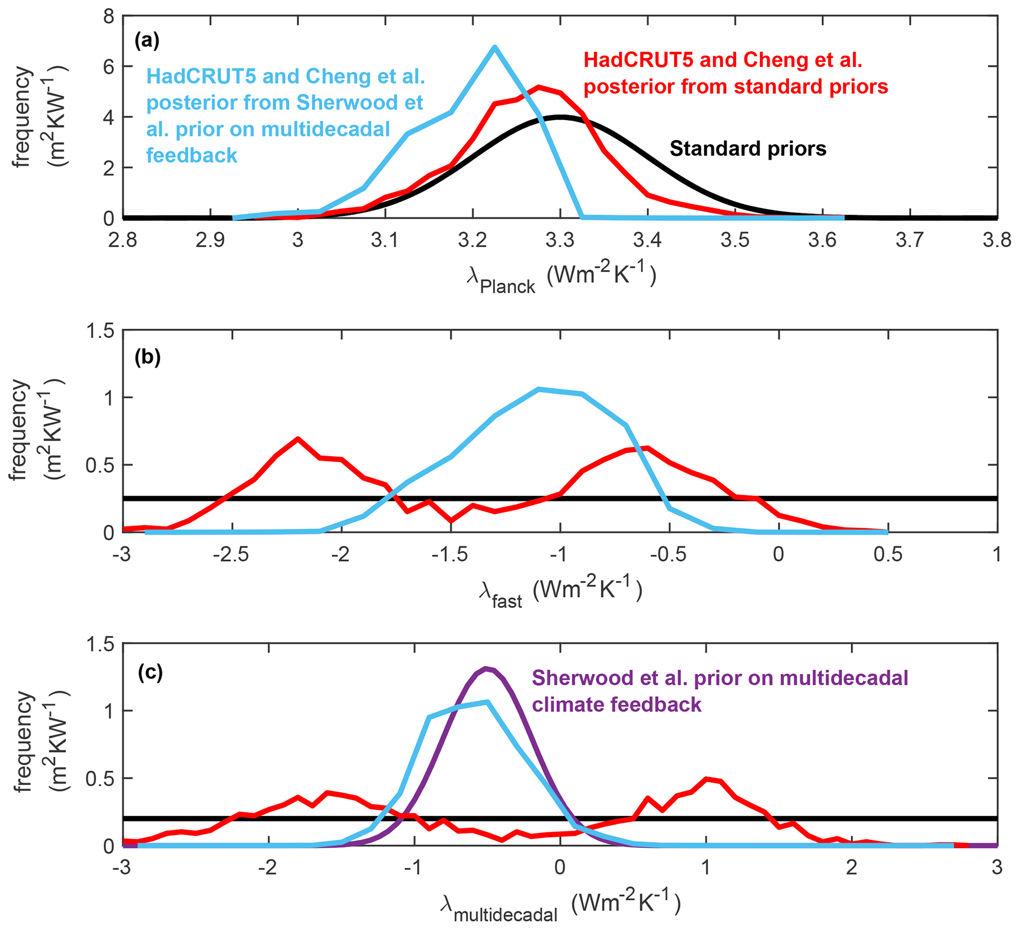
Figure 8 The prior and posterior distribution of climate feedback terms, showing the impact of alternative prior distribution for multi-decadal climate feedback. Black lines show the standard prior distributions (as Fig. 2a–c), while the purple line (c) shows the alternative prior distribution for multi-decadal feedback from Sherwood et al. (2020). Red lines show the posterior in the HadCRUT5 and Cheng et al. ensemble for the standard prior distributions (as Fig. 2a–c), and light blue lines show the posterior distributions for climate feedback terms when using the alternative multi-decadal prior.

These are not the only prior distributions that could have been chosen, and the scatter relationship in Fig. 2d shows that if we constrain either ${\mathit{\lambda }}_{\text{multi-decadal}}^{\text{equil}}$ or ${\mathit{\lambda }}_{\text{fast}}^{\text{equil}}$ then we also constrain the other term. Sherwood et al. (2020) use evidence from a range of sources to justify a Gaussian distribution for the climate feedback due to the pattern effect that amplifies warming over several decades by 0.5 $\mathrm{W}{\mathrm{m}}^{-\mathrm{2}}{\mathrm{K}}^{-\mathrm{1}}$ with a 90 % confidence interval of 0 to 1 $\mathrm{W}{\mathrm{m}}^{-\mathrm{2}}{\mathrm{K}}^{-\mathrm{1}}$. This is equivalent in this study to a normal distribution for ${\mathit{\lambda }}_{\text{multi-decadal}}^{\text{equil}}$ with a mean of −0.5 $\mathrm{W}{\mathrm{m}}^{-\mathrm{2}}{\mathrm{K}}^{-\mathrm{1}}$ and a 90 % confidence range of −1.0 to 0.0 $\mathrm{W}{\mathrm{m}}^{-\mathrm{2}}{\mathrm{K}}^{-\mathrm{1}}$ (Fig. 8c, purple), noting the change in sign convention relative to Sherwood et al. (2020). Since the evidence used by Sherwood et al. (2020) to justify this distribution does not contain the observational constraints used within the likelihood function in this study (Table S2), we are free to adopt the Sherwood et al. (2020) distribution as an alternative prior for ${\mathit{\lambda }}_{\text{multi-decadal}}^{\text{equil}}$ (Fig. 8c, purple). Here, the impact of this alternative prior on our results is explored by weighting the posterior simulations in the HadCRUT5 and Cheng et al. ensemble according to where their ${\mathit{\lambda }}_{\text{multi-decadal}}^{\text{equil}}$ values fit within the Sherwood et al. (2020) prior distribution for multi-decadal climate feedback relative to the uniform prior distribution (Fig. 8c, compare purple and black). Adopting this alternative prior on ${\mathit{\lambda }}_{\text{multi-decadal}}^{\text{equil}}$ (Fig. 8c, purple) does indeed constrain the posterior distributions for both ${\mathit{\lambda }}_{\text{multi-decadal}}^{\text{equil}}$ and ${\mathit{\lambda }}_{\text{fast}}^{\text{equil}}$ (Fig. 8, compare light blue to red). This has only a minor impact on TCR and climate sensitivity on a 20-year timescale (Table 1) but greatly reduces uncertainty in posterior climate sensitivity on 100- and 140-year timescales (Table 1): changing S₁₄₀ from 2.3 (1.6 to 4.2 at 66 % confidence) K with uniform prior to 2.4 (2.0 to 2.8) K with the Sherwood et al. (2020) prior on multi-decadal feedback. This reduction in confidence interval should be expected since the prior for λ_{multi-decadal} has been significantly reduced in range (Fig. 8c, compare black and purple). Full analysis of the impact of alternative priors is reserved for further study.

5 Discussion

Many studies have combined reconstructions of surface temperature and ocean heat uptake with estimates of radiative forcing to calculate the effective climate feedback and/or transient climate response during the historic period (e.g. Annan, 2015; Annan and Hargreaves, 2020; Bodman and Jones, 2016; Lewis and Curry, 2014; Skeie et al., 2018; Otto et al., 2013; Tokarska et al., 2020). However, climate feedback strengths evolve over time in complex climate models (e.g. Andrews et al., 2015), indicating that climate sensitivity values obtained from historic observations may not apply into the future.

This study applies the historic observational record (Table S2) and estimates of historic radiative forcing (Fig. 3; Table S2) to constrain how climate sensitivity evolves on different response timescales (Figs. 4 and 5), utilizing a model of independent climate feedback terms that respond to forcing over instantaneous (Planck), fast (several days), and multi-decadal timescales (Eqs. 2–4). A Bayesian approach is adopted, where uniform prior probability distributions are applied for the fast and multi-decadal climate feedbacks (Fig. 2, Table S1). Different temperature and ocean heat content observational datasets (Table S2, Eqs. 6–8) are applied to extract posterior probability distributions for climate feedbacks (Fig. 2) and other model properties (e.g. related to aerosol radiative forcing Fig. 3). We then use these posterior probability distributions to evaluate climate sensitivity (S) and transient climate response (TCR) from the 4×CO₂ and 1pctCO₂ forcing scenarios, respectively.

Our estimates of S on a 20-year timescale are directly comparable to estimates of climate sensitivity made from historical constraints (e.g. Otto et al., 2013; Lewis and Curry, 2014), without explicitly considering the impact of additional slower (including multi-decadal) climate feedbacks that may not have had time to equilibrate in the present day.

Our estimates of S on 100- and 140-year timescales are directly comparable to the climate sensitivity estimates evaluated in complex climate model simulations from simulations lasting over 100 years, for example using the Gregory et al. (2004) method. Note that additional slow feedbacks not considered here, acting from many decades to millennia, may affect how our estimates are comparable to estimates of climate sensitivity from the palaeo-record where any longer feedbacks have been treated as radiative forcing (e.g. Rohling et al., 2012, 2018).

We find that the HadCRUT5 (Morice et al., 2021) temperature reconstruction implies a larger S and TCR than HadCRUT5 (no infill) (Figs. 4–6; Table 1), demonstrating the importance of statistical infilling of geographical areas absent in historical datasets when constraining future warming (Cowtan and Way, 2014). The Cheng et al. (2017) ocean heat content reconstruction implies similar S to the NODC reconstruction (Figs. 3 and 5; Table 1), showing the insensitivity of our results to these different heat content reconstructions (Fig. 1b). The different heat content datasets make almost no impact on TCR (Fig. 6; Table 1), which may be expected when considering that a larger historic heat content also implies larger heat uptake on a 1pctCO₂ scenario and that this balances any warming impact of a larger S. An alternative narrower prior distribution for multi-decadal climate feedback (Sherwood et al., 2020) reduces uncertainty in our posterior estimates of S on longer, i.e. 100- and 140-year, timescales but has little impact on TCR or S on a 20-year timescale (Table 1, Fig. 8).

Our method constrains S over multiple response timescales (Fig. 4; Table 1). Our constraints on S over 100- and 140-year response timescales (S₁₀₀, S₁₄₀; see Table 1) are directly comparable to previous reviews of climate sensitivity in the literature in AR5 (IPCC, 2013) and Sherwood et al. (2020). The IPCC (2013) AR5 estimate of (“effective” or “equilibrium”) climate sensitivity has a 66 % (or better) likelihood range of 1.5 to 4.5 K (IPCC, 2013), while the recent Sherwood et al. (2020) Bayesian review has a narrower baseline 17th–83rd percentile (66 %) range of 2.6 to 3.6 K. The Sherwood et al. (2020) range removes both the lower portion of the likely IPCC climate sensitivity (66 % likelihood or better) range (from 1.5 to 2.5 K) and the upper portion (from 3.7 to 4.5 K), suggesting a similar best estimate but with reduced uncertainty compared to IPCC (2013).

Our posterior 66 % range for S₁₄₀ (of 1.6 to 4.2 K for our preferred HadCRUT5 and Cheng et al. ensemble) is in very good agreement with the equivalent IPCC (2013) range (Table 1) and is broader than the recent Sherwood et al. (2020) range. Both Sherwood et al. (2020) and this study apply Bayesian approaches to constrain effective climate feedback, λ_eff, and use this constraint on λ_eff to then constrain S. Our broader range compared to Sherwood et al. (2020) may arise from differences in our Bayesian approaches. Firstly, Sherwood et al. (2020) consider additional sources of evidence, for example from palaeoclimate reconstructions, that may narrow their range of climate sensitivity relative to ours. Secondly, our methodology includes a model of climate feedback that is explicitly allowed to evolve over different response timescales (Fig. 2; Eqs. 1–5; Supplement), with equal prior weighting given to amplifying and damping feedback evolution over multi-decadal timescales (Fig. 2b). This time evolution in λ_eff thus allows S to also evolve over different response timescales (Fig. 3, Table 1) and prevents our approach from over-constraining S on multi-decadal and century timescales from historical datasets that record only the decadal responses to recent anthropogenic forcing. When a narrower prior distribution for multi-decadal climate feedback from Sherwood et al. (2020) is adopted within our approach, our posterior S₁₄₀ decreases in range (2.0 to 2.8 K at 66 % confidence; see Table 1) but to lower values than Sherwood et al. (2020). It should be noted that additional slow feedbacks acting on longer timescales (century and longer) may allow climate sensitivity to evolve further (e.g. Rohling et al., 2012, 2018) but are not considered in our methodology.