Comparison of CMIP6 historical climate simulations and future projected warming to an empirical model of global climate

The sixth phase of the Coupled Model Intercomparison Project (CMIP6) is the latest modeling effort for general circulation models to simulate and project various aspects of climate change. Many of the general circulation models (GCMs) participating in CMIP6 provide archived output that can be used to calculate effective climate sensitivity (ECS) and forecast future temperature change based on emissions scenarios from several Shared Socioeconomic Pathways (SSPs). Here we use our multiple linear regression energy balance model, the Empirical Model of Global Climate (EM-GC), to simulate and project changes in global mean surface temperature (GMST), calculate ECS, and compare to results from the CMIP6 multi-model ensemble. An important aspect of our study is a comprehensive analysis of uncertainties due to radiative forcing of climate from tropospheric aerosols (AER RF) in the EM-GC framework. We quantify the attributable anthropogenic warming rate (AAWR) from the climate record using the EM-GC and use AAWR as a metric to determine how well CMIP6 GCMs replicate human-driven global warming over the last 40 years. The CMIP6 multi-model ensemble indicates a median value of AAWR over 1975–2014 of 0.221 ^∘C per decade (range of 0.151 to 0.299 ^∘C per decade; all ranges given here are for 5th and 95th confidence intervals), which is notably faster warming than our median estimate for AAWR of 0.157 ^∘C per decade (range of 0.120 to 0.195 ^∘C per decade) inferred from the analysis of the Hadley Centre Climatic Research Unit version 5 data record for GMST. Estimates of ECS found using the EM-GC assuming that climate feedback does not vary over time (best estimate 2.33 ^∘C; range of 1.40 to 3.57 ^∘C) are generally consistent with the range of ECS of 1.5 to 4.5 ^∘C given by the IPCC's Fifth Assessment Report. The CMIP6 multi-model ensemble exhibits considerably larger values of ECS (median 3.74 ^∘C; range of 2.19 to 5.65 ^∘C). Our best estimate of ECS increases to 3.08 ^∘C (range of 2.23 to 5.53 ^∘C) if we allow climate feedback to vary over time. The dominant factor in the uncertainty for our empirical determinations of AAWR and ECS is imprecise knowledge of AER RF for the contemporary atmosphere, though the uncertainty due to time-dependent climate feedback is also important for estimates of ECS. We calculate the likelihood of achieving the Paris Agreement target (1.5 ^∘C) and upper limit (2.0 ^∘C) of global warming relative to pre-industrial for seven of the SSPs using both the EM-GC and the CMIP6 multi-model ensemble. In our model framework, SSP1-2.6 has a 53 % probability of limiting warming at or below the Paris target by the end of the century, and SSP4-3.4 has a 64 % probability of achieving the Paris upper limit. These estimates are based on the assumptions that climate feedback has been and will remain constant over time since the prior temperature record can be fit so well assuming constant climate feedback. In addition, we quantify the sensitivity of future warming to the curbing of the current rapid growth of atmospheric methane and show that major near-term limits on the future growth of methane are especially important for achievement of the 1.5 ^∘C goal of future warming. We also quantify warming scenarios assuming climate feedback will rise over time, a feature common among many CMIP6 GCMs; under this assumption, it becomes more difficult to achieve any specific warming target. Finally, we assess warming projections in terms of future anthropogenic emissions of atmospheric carbon. In our model framework, humans can emit only another 150±79 Gt C after 2019 to have a 66 % likelihood of limiting warming to 1.5 ^∘C and another 400±104 Gt C to have the same probability of limiting warming to 2.0 ^∘C. Given the estimated emission of 11.7 Gt C per year for 2019 due to combustion of fossil fuels and deforestation, our EM-GC simulations suggest that the 1.5 ^∘C warming target of the Paris Agreement will not be achieved unless carbon and methane emissions are severely curtailed in the next 10 years.

1 Introduction

The goals of the Paris Agreement, negotiated in December of 2015, are to keep global warming below 2.0 ^∘C relative to the start of the Industrial Era and pursue efforts to limit global warming to 1.5 ^∘C. General circulation models (GCMs) project future temperature change using various evolutions of greenhouse gases and determine the likelihood of achieving the goals of the agreement. Many GCMs are participating in the sixth phase of the Coupled Model Intercomparison Project (CMIP6) to quantify how the models represent different aspects of climate change (Eyring et al., 2016). Accurate projections of future temperature are critical for achieving the goals of the Paris Agreement. Chapter 11 of the IPCC's Fifth Assessment Report shows that some of the previous generations of these models participating in phase 5 of the Coupled Model Intercomparison Project (CMIP5) (Taylor et al., 2012) tended to overestimate the increase in global mean surface temperature (GMST) for the 21st century (Kirtman et al., 2013). In this analysis we use a multiple linear regression energy balance model to quantify the change in GMST from 1850–2019, project future changes in GMST, compare to the CMIP6 multi-model ensemble, and determine the likelihood of achieving the goals of the Paris Agreement.

Several prior studies have used a multiple linear regression approach to model the GMST anomaly in order to quantify the impact of anthropogenic and natural factors on climate (Foster and Rahmstorf, 2011; Lean and Rind, 2008, 2009; Zhou and Tung, 2013). Typically, total solar irradiance, volcanoes, and the El Niño–Southern Oscillation (ENSO) are the natural components represented in the multiple linear regression. Greenhouse gases and aerosols are the anthropogenic factors. We use multiple linear regression, in connection with a dynamic ocean module that accounts for the export of heat from the atmosphere to the ocean, to represent the natural and anthropogenic components of the climate system. In addition to the typical natural factors listed above, we include the Atlantic Meridional Overturning Circulation (AMOC), Pacific Decadal Oscillation (PDO), and Indian Ocean Dipole (IOD) to provide a robust representation of the natural climate system (Canty et al., 2013; Hope et al., 2017). Our anthropogenic components also include the effect of land-use change (i.e., deforestation) on Earth's albedo and the export of heat from the atmosphere to the ocean as the atmosphere warms.

Our analysis builds on the work of Canty et al. (2013) and Hope et al. (2017) and includes several key updates. One is the extension back in time of our analysis to 1850. The Hadley Centre Climatic Research Unit (Morice et al., 2012, 2021), Berkeley Earth Group (Rohde and Hausfather, 2020), and Cowtan and Way (2014) provide GMST records starting in 1850, which now allows for simulations of GMST that cover 170 years. The second update is the use of the Shared Socioeconomic Pathways (SSPs) (O'Neill et al., 2017) as our climate scenarios for greenhouse gas and aerosol abundances. The third is the adoption of an upper ocean to our model, formulated in a manner that matches the equations of Bony et al. (2006) and Schwartz (2012). A description of the model, the various input parameters used, and the updates listed above is given in Sect. 2. Section 3 shows results of CMIP6 and EM-GC comparisons to the historical climate record, estimations of effective climate sensitivity (ECS) and comparisons of our model and CMIP6 projections of future GMST change. A discussion of these results is provided in Sect. 4, along with concluding remarks.

2 Data and methodology

2.1 Empirical model of global climate

In this analysis we use the empirical model of global climate (EM-GC), which provides a multiple linear regression energy balance simulation of GMST. As detailed in the following paragraphs, the EM-GC solves for ocean heat uptake efficiency (κ) and six regression coefficients to minimize the cost function in Eq. (1).

$$\begin{array}{}\text{(1)}& \mathrm{Cost}\mathrm{function}=\sum _{i=\mathrm{1}}^{N_{\mathrm{MONTHS}}}{\displaystyle \frac{\mathrm{1}}{{\mathit{\sigma }}_{\mathrm{OBS}i}^{\mathrm{2}}}}{\left(\mathrm{\Delta }{T}_{\mathrm{OBS}i}-\mathrm{\Delta }{T}_{\mathrm{MDL}i}\right)}^{\mathrm{2}}\end{array}$$

In this equation, ΔT_OBS represents a time series of observed monthly GMST anomalies, ΔT_MDL is the modeled monthly change in GMST, σ_OBS is the 1σ uncertainty associated with each temperature observation, i is the index for each month, and N_MONTHS is the total number of months used in the analysis. For this analysis, we trained the model from 1850–2019. The observed GMST anomalies are blended near-surface air and sea surface temperature differences relative to the GMST anomaly over 1850–1900, which is assumed to represent pre-industrial conditions.

We consider several anthropogenic and natural factors to be components of ΔT_MDL. The radiative forcing (RF) due to greenhouse gases (GHGs), anthropogenic aerosols (AER), land-use change (LUC), and the export of heat from the atmosphere to the world's oceans are the anthropogenic components of ΔT_MDL. The influence on GMST from total solar irradiance (TSI), the El Niño–Southern Oscillation (ENSO), the Atlantic Meridional Overturning Circulation (AMOC), volcanic eruptions that reach the stratosphere and enhance stratospheric aerosol optical depth (SAOD), the Pacific Decadal Oscillation (PDO), and the Indian Ocean Dipole (IOD) are the natural components of ΔT_MDL. Equation (2) shows how we calculate ΔT_MDL, the modeled monthly change in GMST.

$$\begin{array}{}\text{(2)}& \begin{array}{rl}& \mathrm{\Delta }{T}_{\mathrm{MDL}i}={\displaystyle \frac{\mathrm{1}+\mathit{\gamma }}{{\mathit{\lambda }}_{\mathrm{P}}}}\left\{\mathrm{GHG}\mathrm{\Delta }{\mathrm{RF}}_i+\mathrm{AER}\mathrm{\Delta }{\mathrm{RF}}_i+\mathrm{LUC}\mathrm{\Delta }{\mathrm{RF}}_i\right.\\ & \left.-Q_{\mathrm{OCEAN}i}\right\}+C_{\mathrm{0}}+C_{\mathrm{1}}\times {\mathrm{SAOD}}_{i-\mathrm{6}}+C_{\mathrm{2}}\times {\mathrm{TSI}}_{i-\mathrm{1}}\\ & +C_{\mathrm{3}}\times {\mathrm{ENSO}}_{i-\mathrm{2}}+C_{\mathrm{4}}\times {\mathrm{AMOC}}_i+C_{\mathrm{5}}\times {\mathrm{PDO}}_i+C_{\mathrm{6}}\\ & \times {\mathrm{IOD}}_i\end{array}\end{array}$$

In Eq. (2), GHG ΔRF_i, AER ΔRF_i, and LUC ΔRF_i represent monthly time series of the increase in the stratospheric adjusted values of the RF of climate (Solomon, 2007) since 1750. The parameter λ_P represents the response of a black body to a perturbation in the absence of climate feedback (3.2 W m⁻²; Bony et al., 2006). The SAOD, TSI, and ENSO are lagged by 6, 1, and 2 months, respectively. The lag of 6 months for SAOD is representative of the time needed for the surface temperature to respond to a change in the aerosol loading due to a volcanic eruption (Douglass and Knox, 2005). This lag is the same as used by Lean and Rind (2008) and Foster and Rahmstorf (2011). The 1-month delay for TSI yields the maximum value of C₂, the solar irradiance regression coefficient. Lean and Rind (2008) and Foster and Rahmstorf (2011) also use a 1-month lag for TSI in their analyses. The 2-month delay for the response of GMST to ENSO is the lag needed to obtain the largest value of the correlation coefficient of the Multivariate ENSO index version 2 (MEI.v2) (Wolter and Timlin, 1993; Zhang et al., 2019) versus the value of T_ENSO calculated by Thompson et al. (2009). In Thompson et al. (2009), T_ENSO is the simulated response of GMST to variability induced by ENSO, taking into consideration the effective heat capacity of the atmospheric–ocean mixed layer. Lean and Rind (2008) used a 4-month lag for ENSO.

The term AMOC_i represents the influence of the change in the strength of the thermohaline circulation on GMST (Knight et al., 2005; Medhaug and Furevik, 2011; Stouffer et al., 2006; Zhang and Delworth, 2007). We use the Atlantic multidecadal variability, based on the area-weighted monthly mean sea surface temperature (SST) in the Atlantic Ocean between the Equator and 60^∘ N (Schlesinger and Ramankutty, 1994), as a proxy for the strength of AMOC. A strong AMOC is characterized by northward flow of energy that would otherwise be radiated to space, which occurs in both the ocean and atmosphere and leads to particularly warm summers in Europe (Kavvada et al., 2013) as well as a number of other well-documented influences in other climatic regions (Nigam et al., 2011). The total anthropogenic RF is used to detrend the AMOC signal. This method provides a more realistic approach to infer the changes in the strength of the AMOC and its effect on GMST than other detrending options (Canty et al., 2013).

The dimensionless parameter γ represents the sensitivity of the global climate to feedbacks that occur due to a change in the RF of GHGs, AER, and LUC. We relate γ to the climate feedback parameter, λ_Σ, as shown in Eq. (3):

$$\begin{array}{}\text{(3)}& \mathrm{1}+\mathit{\gamma }={\displaystyle \frac{\mathrm{1}}{\mathrm{1}-\left(\frac{{\mathit{\lambda }}_{\mathrm{\Sigma }}}{{\mathit{\lambda }}_{\mathrm{P}}}\right)}},\end{array}$$

where λ_Σ=Σ for all climate feedbacks, i.e., ${\mathit{\lambda }}_{\mathrm{\Sigma }}={\mathit{\lambda }}_{\mathrm{Water}\mathrm{vapor}}+{\mathit{\lambda }}_{\mathrm{Lapse}\mathrm{rate}}+{\mathit{\lambda }}_{\mathrm{Clouds}}+{\mathit{\lambda }}_{\mathrm{Surface}\mathrm{albedo}}$. The relation between λ_Σ and γ in Eq. (3) is commonly used in the climate modeling community (Sect. 8.6 of Solomon, 2007). Our value of λ_Σ is related to the IPCC's Fifth Assessment Report (Stocker et al., 2013; hereafter IPCC 2013) definition of λ via ${\mathit{\lambda }}_{\mathrm{\Sigma }}={\mathit{\lambda }}_{\mathrm{P}}-\mathit{\lambda }$.

Our model explicitly accounts for the export of heat from the atmosphere to the world's oceans (i.e., ocean heat export or OHE). The quantity Q_OCEAN in Eq. (2) represents OHE. In our previous analyses (Canty et al., 2013; Hope et al., 2017), Q_OCEAN was subtracted outside the climate feedback multiplicative term $(\mathrm{1}+\mathit{\gamma })/{\mathit{\lambda }}_{\mathrm{P}}$. We have rewritten Eq. (2) to be comparable to the formulation for this term used by Bony et al. (2006) and Schwartz (2012). Due to this update, our model fits the historical climate record with higher values of climate feedback, especially for strong aerosol cooling (see Fig. S1 and the Supplement for more information). We calculate Q_OCEAN by simulating the long-term trend in observed ocean heat content (OHC) as shown in Eqs. (4) and (5).

$$\begin{array}{}\text{(4)}& {\displaystyle }{Q}_{\mathrm{OCEAN}i}=\mathit{\kappa }\left(\mathrm{\Delta }{T}_{\mathrm{ATM},\mathrm{HUMAN}i}-\mathrm{\Delta }{T}_{\mathrm{OCEAN},\mathrm{HUMAN}i}\right)\text{(5)}& {\displaystyle }\mathit{\kappa }={\displaystyle \frac{\mathrm{OHE}\times \mathrm{\Delta }t}{\begin{array}{c}{\int }_{t_{\mathrm{START}}}^{t_{\mathrm{END}}}\left(\left[\frac{\mathrm{1}+\mathit{\gamma }}{{\mathit{\lambda }}_{\mathrm{P}}}\left\{\mathrm{GHG}{\mathrm{RF}}_{i-\mathrm{72}}+\mathrm{AER}{\mathrm{RF}}_{i-\mathrm{72}}\right.\right.\right.\\ \left.\left.\left.+\mathrm{LUC}{\mathrm{RF}}_{i-\mathrm{72}}\right\}\right]-\left[f_{\mathrm{0}}{\sum }_{\mathrm{0}}^{i-\mathrm{72}}{Q}_{\mathrm{OCEAN}}\right]\right)\mathrm{d}t\end{array}}}\end{array}$$

The κ term is the ocean heat uptake efficiency (W m^−2 ∘C⁻¹) and is based on the definition used in Raper et al. (2002), where κ is the ratio between the atmosphere and ocean temperature difference that best fits observed OHC data (Sect. 2.2.8 describes the OHC data records used in our analysis). The value of κ is determined based on the best fit (described below) between Q_OCEAN and the observed OHC record. The term ΔT_OCEAN,HUMAN represents the temperature response of the well-mixed top 100 m of the ocean due to the total anthropogenically driven rise in OHC. This formulation of ΔT_OCEAN,HUMAN allows the model ocean to warm in response to an atmospheric warming. We use a 6-year lag (72 months) for Q_OCEAN to account for the time needed for the energy leaving the atmosphere to heat the upper ocean and penetrate to depth based on Schwartz (2012). Our analysis of modeled GMST is insensitive to whether this 6-year lag or the 10-year lag from Lean and Rind (2009) is used. The t_START and t_END limits on the integral in Eq. (5) are the start and end years associated with each OHC record. The start and end years vary between the five OHC records (see the Supplement for the different start and end years). The constant f₀ term in Eq. (5) is a combination of the heat capacity of ocean water, the fraction of total ocean volume in the surface layer, and the fraction of total Q_OCEAN that warms the surface layer; it is equal to $\mathrm{8.76}\times {\mathrm{10}}^{-\mathrm{5}}$ ^∘C m² W⁻¹. We represent the global ocean as being 1 km deep for 10 % of the ocean area (representing the continental shelves) and 4 km deep for the remaining area, which approximates the average depth of the actual world's oceans to within 3 %: 3.7 km compared to 3.682–3.814 km from Charette and Smith (2010). Based on our analysis of decadal ocean warming as a function of depth extracted from CMIP5 GCMs, we have determined that 13.7 % of the rise in total OHC occurs in the well-mixed upper 100 m of the ocean, the term represented by ΔT_OCEAN,HUMAN in Eq. (4). The bottom panel in Fig. 1 compares our modeled OHC to the observed OHC record based on the average of five data sets; the value of κ resulting in the best simulation of observed OHC is shown.

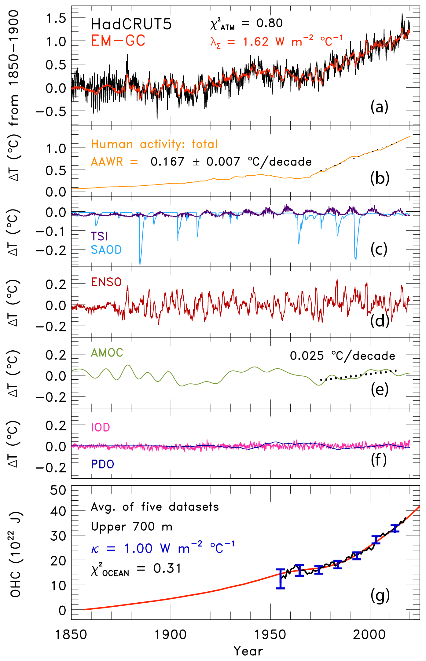
Figure 1 Measured and modeled GMST anomaly (ΔT) relative to a pre-industrial (1850–1900) baseline. (a) Observed (black) HadCRUT5 and modeled (red) ΔT from 1850–2019. This panel also displays the values of λ_Σ and ${\mathit{\chi }}_{\mathrm{ATM}}^{\mathrm{2}}$ (see text) for this best-fit simulation. (b) Contributions from total human activity. This panel also denotes the best-estimate value of the attributable anthropogenic warming rate from 1975–2014 (black dashed) and the 2σ uncertainty in the slope for a model run that uses the best estimate of AER RF₂₀₁₁ of −0.9 W m⁻². (c) TSI (purple) and SAOD (light blue). (d) Influences from ENSO on ΔT. (e) Contributions from AMOC to ΔT and to observed warming from 1975–2014. (f) Influences from PDO (blue) and IOD (pink) on ΔT. (g) Measured (black) and modeled (red) ocean heat content (OHC) as a function of time for the average of five data sets (see text), the value of ${\mathit{\chi }}_{\mathrm{OCEAN}}^{\mathrm{2}}$ for this run, and the ocean heat uptake efficiency, κ, needed to provide the best fit to the OHC record. The error bars (blue) denote the uncertainty in OHC used in this analysis (see Sect. 2.2.8).

We use the reduced chi-squared (χ²) metric to define the goodness of fit between the modeled and measured GMST anomaly for the atmosphere and also between simulated and observed OHC. Equations (6) and (7) show the calculations for χ² for the atmosphere, and Eq. (8) shows the calculation for χ² for the ocean. Minimization of the difference between the measured and modeled GMST anomaly results in the EM-GC being able to replicate the observed rise in temperature over the past 170 years quite well, as shown in Fig. 1. We have added two additional new features to the model to ensure accurate representation of the rise in OHC and the rise in GMST since 1940. The first new feature, Eq. (7), was added to ensure all simulations matched the past 80 years of observations well. Without the ${\mathit{\chi }}_{\mathrm{RECENT}}^{\mathrm{2}}$ constraint, some solutions with a value of ${\mathit{\chi }}_{\mathrm{ATM}}^{\mathrm{2}}$ less than or equal to 2 have visually poor simulations of the rise in GMST over the past 4 to 5 decades. The second new feature, Eq. (8), was added because in the original model formulation some selections of the radiative forcing due to tropospheric aerosols (AER ΔRF_i in Eq. 2) converged in a way that produced simulations of OHC that seemed physically improper based on visual inspection of observed and modeled OHC. As a result of these two issues, all calculations shown here are subject to three goodness-of-fit constraints described by Eqs. (6) to (8).

$$\begin{array}{}\text{(6)}& {\displaystyle }\begin{array}{rl}{\mathit{\chi }}_{\mathrm{ATM}}^{\mathrm{2}}& ={\displaystyle \frac{\mathrm{1}}{N_{\mathrm{YEARS}}-N_{\mathrm{FITTING}\mathrm{PARAMETERS}}-\mathrm{1}}}\\ & \times \sum _{j=\mathrm{1}}^{N_{\mathrm{YEARS}}}{\displaystyle \frac{\mathrm{1}}{\langle {\mathit{\sigma }}_{\mathrm{OBS}j}{\rangle }^{\mathrm{2}}}}(\langle \mathrm{\Delta }{T}_{\mathrm{OBS}j}\rangle -\langle \mathrm{\Delta }{T}_{\mathrm{MDL}j}\rangle {)}^{\mathrm{2}}\end{array}\text{(7)}& {\displaystyle }\begin{array}{rl}{\mathit{\chi }}_{\mathrm{RECENT}}^{\mathrm{2}}& ={\displaystyle \frac{\mathrm{1}}{N_{\mathrm{YEARS},\mathrm{REC}}-N_{\mathrm{FITTING}\mathrm{PARAMETERS}}-\mathrm{1}}}\\ & \times \sum _{j=\mathrm{1}}^{N_{\mathrm{YEARS},\mathrm{REC}}}{\displaystyle \frac{\mathrm{1}}{\langle {\mathit{\sigma }}_{\mathrm{OBS}j}{\rangle }^{\mathrm{2}}}}(\langle \mathrm{\Delta }{T}_{\mathrm{OBS}j}\rangle -\langle \mathrm{\Delta }{T}_{\mathrm{MDL}j}\rangle {)}^{\mathrm{2}}\end{array}\text{(8)}& {\displaystyle }\begin{array}{rl}& {\mathit{\chi }}_{{\mathrm{OCEAN}}^{\mathrm{2}}}={\displaystyle \frac{\mathrm{1}}{N_{\mathrm{YEARS}}-N_{\mathrm{FITTING}\mathrm{PARAMETERS}}-\mathrm{1}}}\\ & \times \sum _{j=\mathrm{1}}^{N_{\mathrm{YEARS},\mathrm{OHC}}}{\displaystyle \frac{\mathrm{1}}{\langle {\mathit{\sigma }}_{\mathrm{OBS}j}{\rangle }^{\mathrm{2}}}}(\langle {\mathrm{OHC}}_{\mathrm{OBS}j}\rangle -\langle {\mathrm{OHC}}_{\mathrm{MDL}j}\rangle {)}^{\mathrm{2}}\end{array}\end{array}$$

Here, <ΔT_OBS>, <ΔT_MDL>, and <σ_OBS> in Eqs. (6) and (7) represent the annually averaged observed GMST anomaly, modeled GMST anomaly, and uncertainty in the GMST anomaly, respectively. The variable N_{FITTING PARAMETERS} is equal to 9 for typical simulations, the sum of 7 (the number of regression coefficients) plus 2 (model output parameters γ and κ). In Eq. (8), <OHC_OBS> and <OHC_MDL> represent the annual averaged observed and modeled OHC. The σ_OBS term in Eq. (8) is the uncertainty in the OHC record (see Sect. 2.2.8 for more information). The equation for all three formulations of χ² is based on annual averages rather than monthly time series. We calculate χ² with annual values because the autocorrelation functions of ΔT_OBS and ΔT_MDL display similar shapes using annual averages and do not match utilizing monthly averages (see the Supplement of Canty et al., 2013, for a further explanation). The Hadley Centre Climate Research Unit (HadCRUT) version 4 uncertainties for GMST are used for the σ_OBS in Eqs. (6) to (8) for all of the GMST records analyzed here (see Sect. 2.2.1 and the Supplement for more information). For Eqs. (6) to (8), we define an acceptable fit to the climate record as χ²≤2. The number of years (N_YEARS) varies across the three equations. Equation (6) uses the total number of years in the GMST record, which for HadCRUT5 is 170 years. The number of years in Eq. (8), N_YEARS,OHC, depends on the OHC data set used, as each data set spans a different range. The average of five OHC data sets, which we use as our primary OHC series, extends from 1955–2017, a total of 63 years. The value of ${\mathit{\chi }}_{\mathrm{OCEAN}}^{\mathrm{2}}$ found using Eq. (8) is displayed in the bottom panel of Fig. 1. All model simulations shown throughout this paper have ${\mathit{\chi }}_{\mathrm{OCEAN}}^{\mathrm{2}}\le \mathrm{2}$, representing a good fit to the observed rise in OHC over the time of the data record.

The calculation of ${\mathit{\chi }}_{\mathrm{RECENT}}^{\mathrm{2}}$ shown in Eq. (7) is used to constrain the model to match the observed changes in GMST over the time frame 1940–2019, a total of 80 years (N_YEARS,REC equals 80). This time frame was chosen to include a full cycle of AMOC, as the strength of the thermohaline circulation tends to vary on a period of 60–80 years (Chen and Tung, 2018; Kushnir, 1994; Schlesinger and Ramankutty, 1994). As noted above, the ${\mathit{\chi }}_{\mathrm{RECENT}}^{\mathrm{2}}$ constraint was added to our model framework because without this constraint the model is able to provide numerically good but poor visual fits to the GMST anomaly under certain conditions (i.e., the red line in the top panel of Fig. 1 starts to strongly deviate from the black line beginning in about 2000 under certain conditions). All model simulations shown below have ${\mathit{\chi }}_{\mathrm{RECENT}}^{\mathrm{2}}\le \mathrm{2}$, representing a good fit to the observed rise in GMST over the past 80 years, which results in modeled GMST that replicates observed GMST for the entire time series.

Figure 1 shows the observed (HadCRUT5) and modeled GMST anomaly from 1850–2019 and the various anthropogenic and natural components that constitute modeled GMST. Figure 1a shows the value of climate feedback, 1.62 W m^−2 ∘C⁻¹, that is needed to achieve a best fit to the climate record for this simulation, resulting in values of ${\mathit{\chi }}_{\mathrm{ATM}}^{\mathrm{2}}=\mathrm{0.80}$ and ${\mathit{\chi }}_{\mathrm{OCEAN}}^{\mathrm{2}}=\mathrm{0.31}$. Figure 1b is the total contribution of human activity to variations in GMST, which includes GHGs, AER, LUC, and the export of heat from the atmosphere to the ocean. For the simulation shown, the aerosol radiative forcing is −0.9 W m⁻², the best estimate given by IPCC 2013 (Myhre et al., 2013). This panel also notes the best estimate of the time rate of change in GMST attributed to humans from 1975–2014, or the attributable anthropogenic warming rate (AAWR; see Sect. 2.3). Figure 1c illustrates the contribution to the GMST anomaly from TSI and SAOD over the 170-year period. The influences of ENSO and AMOC are indicated in Fig. 1d and e, respectively. Furthermore, the contribution of AMOC to the rise in GMST over 1975–2014 (the same time period used to define AAWR) is also specified in Fig. 1e (dotted black line). Figure 1f indicates the small effect of IOD and PDO on GMST in our model framework. The last panel, Fig. 1g, shows the time series of observed OHC based on the average of five data sets for the upper 700 m of the ocean (black points and blue error bars; see Sect. 2.2.8) and the modeled value of OHC (red line). For this simulation, a value of κ equal to 1.17 W m^−2 ∘C⁻¹ fits the OHC data best. This value of κ falls within the range of empirical estimates for this parameter given by Raper et al. (2002). The sum of the contributions of human activity, TSI, SAOD, ENSO, AMOC, PDO, and IOD to the GMST anomaly shown in Fig. 1b to f plus the value of C₀ equals the modeled GMST anomaly, shown by the red line in Fig. 1a.

Altering the training period of our model has a slight effect on our results (see Figs. S2, S3, and the Supplement for information on various training periods). We project relatively similar results for end-of-century warming for training periods that start in 1850 and end in either 2009 or 1999 compared to results shown throughout the paper for a training period of 1850 to 2019, indicating the stability of our approach. As detailed in the Supplement, we do find some differences from the results shown in the paper upon use of a training period of 1850 to 1989 due to the reduction in the number of years considered from the available OHC records.

2.2 Model inputs

2.2.1 Temperature data

We use seven global mean surface temperature anomaly records. These records include the Hadley Centre Climatic Research Unit version 4 (HadCRUT4; Morice et al., 2012) and version 5 (HadCRUT5; Morice et al., 2021) from 1850–2019, National Centers for Environmental Information NOAAGlobalTemp v5 (NOAAGT; Smith et al., 2008; Zhang et al., 2019) from 1880–2019, NASA Goddard Institute of Space Studies Surface Temperature Analysis v4 (GISTEMP; Hansen et al., 2010) from 1880–2019, Berkeley Earth Group (BEG; Rohde and Hausfather, 2020) from 1850–2019, Cowtan and Way (2014) (CW14) from 1850–2019, and the Japanese Meteorological Agency (JMA; Ishihara, 2006) from 1891–2019. We use the uncertainty time series from HadCRUT4 for all GMST records because the HadCRUT4 uncertainty provides a realistic description of the variation in GMST among the seven records (see the Supplement, Figs. S4 and S5, and Table S1 for more information). Our analysis primarily uses the HadCRUT5 GMST data set, but in some sections, results are shown for the other data sets. All temperature anomalies are with respect to a pre-industrial baseline (1850–1900). To alter each data record so that the temperature anomaly is relative to the same pre-industrial baseline, we adjust all data sets relative to the HadCRUT5 baseline of 1961–1990. We then adjust each data set by the same amount to the HadCRUT5 pre-industrial baseline as described in the Supplement.

2.2.2 Shared Socioeconomic Pathways

For this analysis, we use the estimates of the future abundances of greenhouse gases and aerosols provided by the SSPs. There are 26 scenarios, five baseline pathways, and 21 mitigation scenarios. The baseline pathways follow specific narratives for factors such as population, education, economic growth, and technological developments of sources of renewable energy (Calvin et al., 2017; Fricko et al., 2017; Fujimori et al., 2017; Kriegler et al., 2017; van Vuuren et al., 2017) to represent several possible futures encompassing different challenges for adaptation to and mitigation of climate change as illustrated in Fig. 1 of O'Neill et al. (2014). The 21 mitigation scenarios follow one of the baseline pathways but include specific climate policy to reach a designated radiative forcing at the end of the century.

As part of CMIP6, the ScenarioMIP experiment (O'Neill et al., 2016) includes eight SSPs (SSP1-1.9, SSP1-2.6, SSP4-3.4, SSP2-4.5, SSP4-6.0, SSP3-7.0, SSP5-8.5, and SSP5-3.4-OS) that GCMs use to project future GMST. The first number is the reference pathway that the scenario follows (i.e., SSP1 follows the first SSP narrative), and the numbers after the dash are the target radiative forcing at the end of the century (i.e., SSP1-2.6 reaches around 2.6 W m⁻² in 2100). The ScenarioMIP experiment designates Tier 1 and Tier 2 scenarios. The Tier 1 scenarios are SSP1-2.6, SSP2-4.5, SSP3-7.0, and SSP5-8.5, and the Tier 2 scenarios are SSP1-1.9, SSP4-3.4, SSP4-6.0, and SSP5-3.4-OS (an overshoot pathway that follows SSP5-8.5 until around 2040, whereby carbon dioxide emissions drastically decrease and become negative in 2065). Our analysis includes seven of the eight ScenarioMIP SSPs: all but the overshoot pathway. We highlight four in the main paper: two Tier 1 (SSP1-2.6 and SSP2-4.5) and two Tier 2 (SSP1-1.9 and SSP4-3.4) scenarios. An analysis of the other three SSPs is included in the Supplement. Figure 2 shows the atmospheric abundance of the three major anthropogenic GHGs (carbon dioxide, methane, and nitrous oxide) for each of the seven SSPs we consider and observations of the global mean atmospheric abundance for these gases to the end of 2019 (Dlugokencky, 2020; Dlugokencky and Tans, 2020).

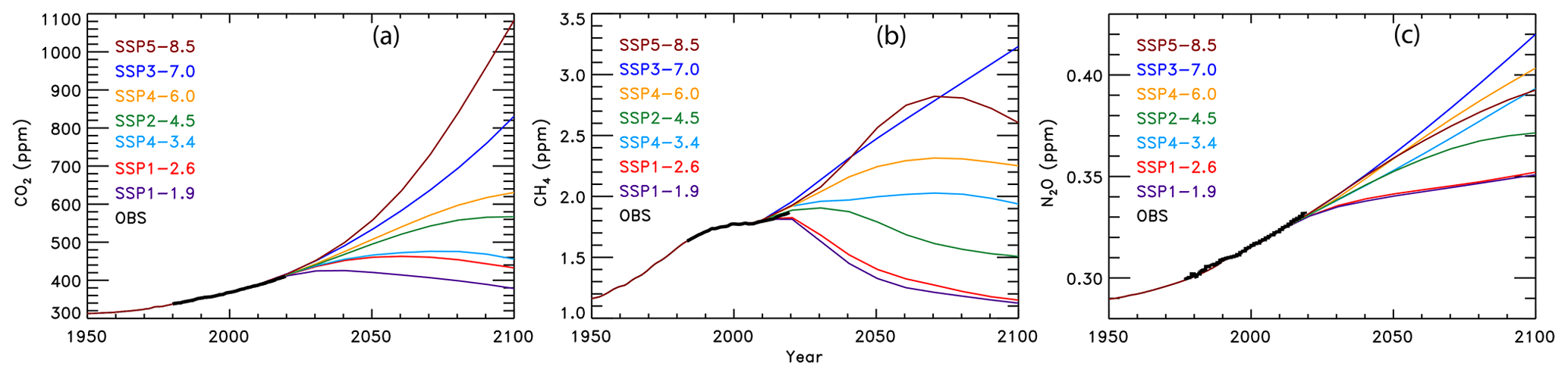
Figure 2 Observed and projected greenhouse gas mixing ratios. (a) Carbon dioxide abundances from observations (black) and seven of the ScenarioMIP SSPs (colors, as indicated). (b) Methane abundances from observations and ScenarioMIP SSPs. (c) Nitrous oxide abundances from observations and ScenarioMIP SSPs.

2.2.3 Greenhouse gases

The historical values of GHG mixing ratios were provided by Meinshausen et al. (2017b) from 1850–2014. We used the equations from Myhre (1998) to calculate the change in RF due to carbon dioxide (CO₂), methane (CH₄), nitrous oxide (N₂O), ozone-depleting substances (ODSs), hydrofluorocarbons, perfluorocarbons, and sulfur hexafluoride relative to RF in the year 1850. We also used the updated pre-industrial values of CH₄ and N₂O from IPCC 2013 and the radiative efficiencies from the WMO (2018). The radiative forcing of CH₄ also includes the 15 % enhancement from the increase in stratospheric water vapor due to rising atmospheric CH₄ (Myhre et al., 2007). Values of GHG mixing ratios, other than ODSs, from 2015–2100 are from the SSP database (Calvin et al., 2017; Fricko et al., 2017; Fujimori et al., 2017; Kriegler et al., 2017; Rogelj et al., 2018; van Vuuren et al., 2017) and are provided on a decadal basis. These mixing ratios were interpolated onto a monthly timescale. We used the estimates of future ODS abundances provided in Table 6-4 of the 2018 Ozone Assessment Report (Carpenter et al., 2018) because the SSP database did not provide these estimates. We also include tropospheric ozone (O${}_{\mathrm{3}}^{\mathrm{TROP}}$) as a GHG because tropospheric ozone rivals N₂O as the third most important anthropogenic GHG (Fig. 8.15 of Myhre et al., 2013). The RF due to O${}_{\mathrm{3}}^{\mathrm{TROP}}$ from the Representative Concentration Pathways (RCPs) provided by the Potsdam Institute for Climate Impact Research (Meinshausen et al., 2011) is used because the SSP database does not provide estimates. Values of RF due to O${}_{\mathrm{3}}^{\mathrm{TROP}}$ from RCP2.6, RCP4.5, RCP6.0, and RCP8.5 are substituted in for SSP1-2.6, SSP2-4.5, SSP4-6.0, and SSP5-8.5, respectively. We created new time series for the RF due to O${}_{\mathrm{3}}^{\mathrm{TROP}}$ for SSP4-3.4 and SSP3-7.0 using linear combinations of RF time series from RCP2.6 and RCP8.5, with weights based on the end-of-century total RF value due to all GHGs of the respective time series. Finally, the RF time series for O${}_{\mathrm{3}}^{\mathrm{TROP}}$ from RCP2.6 was also used for SSP1-1.9. Figure S6 shows the ozone RF time series used in this analysis, and the Supplement provides more information about the creation of the time series for the RF due to O${}_{\mathrm{3}}^{\mathrm{TROP}}$.

2.2.4 Aerosol radiative forcing

The value of the change in total aerosol radiative forcing (direct and indirect) in 2011 relative to pre-industrial (AER RF₂₀₁₁) is highly uncertain. Chapter 8 of the IPCC 2013 report gives a best estimate of AER RF₂₀₁₁ as −0.9 W m⁻², a likely range between −0.4 and −1.5 W m⁻², and a 5th to 95th percent confidence interval between −0.1 and −1.9 W m⁻² (Myhre et al., 2013). This substantial range in AER RF₂₀₁₁ results in a large spread in future projections of global GMST. Figure 3 shows the effect of varying the value of AER RF₂₀₁₁ on projections of GMST in our EM-GC framework for the same SSP4-3.4 GHG scenario. The middle box in Fig. 3a, b, and c shows the contribution to GMST of GHGs, LUC, AER, and net human activities. As the value of AER RF₂₀₁₁ decreases and aerosols cool more strongly, the value of climate feedback (model parameter λ_Σ) rises, and the net contribution of the human impact on GMST by the end of the century increases. Depending on which value of AER RF₂₀₁₁ is used, the rise in GMST by the year 2100 for the SSP4-3.4 pathway could range from 1.5 ^∘C (Fig. 3a) to 2.8 ^∘C (Fig. 3c) relative to pre-industrial. Strong aerosol cooling offsets a substantial fraction of GHG-induced warming, and a large value of climate feedback (λ_Σ=2.41 W m^−2 ∘C⁻¹) is needed to fit the historical climate record (Fig. 3c). In this case, future warming is large, well above the goals of the Paris Agreement, by the end of the century. Conversely, weak aerosol cooling offsets only a small fraction of GHG-induced warming, resulting in a small value of climate feedback (λ_Σ=1.08 W m^−2 ∘C⁻¹) needed to fit the observed GMST record (Fig. 3a). The use of any of the values of AER RF₂₀₁₁ in Fig. 3 can result in a very good fit to the climate record (i.e., ${\mathit{\chi }}_{\mathrm{ATM}}^{\mathrm{2}}\le \mathrm{2}$, ${\mathit{\chi }}_{\mathrm{RECENT}}^{\mathrm{2}}\le \mathrm{2}$, and ${\mathit{\chi }}_{\mathrm{OCEAN}}^{\mathrm{2}}\le \mathrm{2}$).

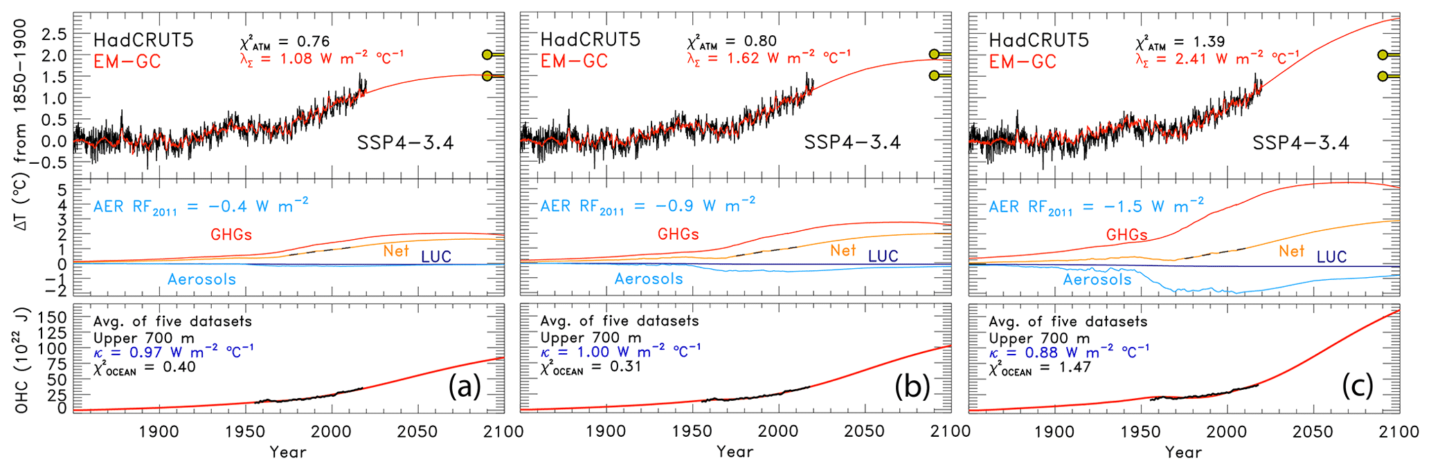
Figure 3 Measured (HadCRUT5) and EM-GC simulated GMST anomaly (ΔT) relative to a pre-industrial (1850–1900) baseline, as well as projected ΔT to the end of the century for SSP4-3.4. The top box in each panel displays observed (black) and simulated (red) ΔT, as well as the values of λ_Σ and ${\mathit{\chi }}_{\mathrm{ATM}}^{\mathrm{2}}$ for each model run. The Paris Agreement target (1.5 ^∘C) and upper limit (2.0 ^∘C) are shown (gold circles). The middle boxes show the contribution of GHGs, aerosols, and land-use change to ΔT, as well as the net human component. The bottom boxes compare observed (black) and modeled (red) values of OHC for simulations constrained by the average of five data sets (see text) and also provides the numerical values of κ needed to obtain best fits to the OHC record as well as best-fit values of ${\mathit{\chi }}_{\mathrm{OCEAN}}^{\mathrm{2}}$. The only difference between (a), (b), and (c) is the time series for RF due to tropospheric aerosols used to constrain the EM-GC; values of AER RF₂₀₁₁ for each time series are (a) −0.4 W m⁻², (b) −0.9 W m⁻², and (c) −1.5 W m⁻².

We use the total aerosol RF time series provided by the SSP database for each SSP scenario. The database provides AER RF from 2005–2100, with values for all SSPs nearly identical until about 2010 (Riahi et al., 2017; Rogelj et al., 2018). In the EM-GC, we calculate temperature projections over the entire observational period beginning in 1850. We create AER RF time series that begin in 1850 and span the range of uncertainty given by Chapter 8 of IPCC 2013. We use historical estimates of AER RF from 1850–2014 for the four RCPs provided by the Potsdam Institute for Climate Research (Meinshausen et al., 2011). The AER RF value in 2014 from the appropriate historical estimate (i.e., RCP4.5 is used for SSP2-4.5) is scaled by a constant factor such that the historical RCP value at the end of 2014 matches the SSP time series at the start of 2015. This scaling yields a continuous time series for the RF of climate due to tropospheric aerosols. This scaled time series has AER RF₂₀₁₁ nearly equal to −1.0 W m⁻², which we take as the SSP-based best estimate of the change in total aerosol radiative forcing in 2011 relative to pre-industrial. Next, the single continuous time series is scaled, again by a constant multiplicative factor, to match the IPCC 2013 best estimate and range of uncertainty for AER RF₂₀₁₁ (Myhre et al., 2013). This procedure results in five additional time series of AER RF. Six time series of AER RF are created for each SSP, having values of AER RF₂₀₁₁ equal to −0.1, −0.4, −0.9, −1.0, −1.5, and −1.9 W m⁻². Figure S7 shows these six AER RF time series for SSP1-2.6 and SSP4-3.4. In the EM-GC framework, we further scale these six time series to create a total of 400 AER RF time series to fully analyze the range of AER RF₂₀₁₁ given by Myhre et al. (2013).

2.2.5 Total solar irradiance and stratospheric aerosol optical depth

We use the TSI time series provided for the CMIP6 models from 1850–2014 (Matthes et al., 2017) and append values from the Solar Radiation and Climate Experiment (SORCE) (Dudok de Wit et al., 2017) for 2015 to the end of 2019. The values of TSI_i used in Eq. (2) are differences of monthly mean values minus the long-term average (i.e., TSI anomalies). Consistent with prior studies (e.g., Lean and Rind, 2008; and Foster and Rahmstorf, 2011), variations in solar irradiance due to the 11-year solar cycle have a small but noticeable effect on the EM-GC simulation of the GMST anomaly (Fig. 1c). For projections of future warming, we set the term TSI_i in Eq. (2) equal to zero from the start of 2020 until 2100.

The time series for SAOD is a combination of values computed from extinction coefficients for the CMIP6 GCMs (Arfeuille et al., 2014) from 1850–1978 and the Global Space-based Stratospheric Aerosol Climatology (GloSSAC v2.0) (Thomason et al., 2018) from 1979–2018. Extinction coefficients at 550 nm were integrated from the tropopause to 39.5 km and averaged over the globe using a cosine of latitude weighting. The CMIP6 and GloSSAC extinction coefficients span 80^∘ S to 80^∘ N. To extend the SAOD time series to the end of 2019, we use the level 3 gridded SAOD product from the Cloud–Aerosol Lidar and Infrared Pathfinder Satellite Observations (CALIPSO) (Vaughan et al., 2004). Time series of globally averaged SAOD from CALIPSO have a very similar shape as the GloSSAC time series over the period of overlap (2006–2018) with a slight offset because GloSSAC uses estimates of CALIPSO data for SAOD. To append the SAOD after 2018, we took the average difference between the two time series for the overlapping months and then adjusted the CALIPSO time series by this offset. This slight adjustment to the CALIPSO record has no bearing on our results, since the effect of volcanic activity on GMST has been small over the past 2 decades (Fig. 1c). We set the term SAOD_i in Eq. (2) equal to the value in December 2019 from the start of 2020 until 2100.

2.2.6 El Niño–Southern Oscillation, Pacific Decadal Oscillation, and Indian Ocean Dipole

We use the MEI.v2 (Wolter and Timlin, 1993; Zhang et al., 2019) to characterize the influence of ENSO on GMST. In order to obtain a time series that spans the entire training period of our model, 1850–2019, we append three time series to create an MEI.v2 over the full extent of our model training period. The MEI.v2 provides 2-month averages of empirical orthogonal functions of five different climatic variables from 1979 to the present (Zhang et al., 2019). To have the ENSO index extend back to 1850, we compute differences in SST anomalies over the tropical Pacific basin as defined by the MEI.v2 from 1850–1870 using HadSST3 (Kennedy et al., 2011). Our internal computation of this surrogate for the MEI is then appended to the MEI.ext of Wolter and Timlin (2011), which extends from 1871–1978, and the MEI.v2 of (Zhang et al., 2019) (1979–2019). This full time series provides a representation of ENSO that covers 1850 to the present. Consistent with prior regression-based approaches (Foster and Rahmstorf, 2011; Lean and Rind, 2008), we find that a significant portion of the monthly and at times annual variation in GMST is well explained by ENSO (Fig. 1d). As for the other natural terms, we assume ENSO_i in Eq. (2) is zero for 2020–2100.

The Pacific Decadal Oscillation is the leading principal component of North Pacific monthly SST variability poleward of 20^∘ N (Barnett et al., 1999). The PDO index maintained by the University of Washington provides monthly values from 1900–2018. The PDO varies on a multidecadal timescale and affects climate in the North Pacific and North America, and it has secondary effects in the tropics (Barnett et al., 1999). In our model framework, the expression of PDO on GMST is dependent on the model specification of the AER RF time series, as shown in Fig. S8. At low values of AER RF₂₀₁₁, such as −0.1 W m⁻², the effect of PDO on GMST is negligible and the contribution from the AMOC dominates. At high values of AER RF₂₀₁₁ (−1.5 W m⁻²), the effect of PDO on GMST is equal to the contribution from the AMOC. At high values of AER RF₂₀₁₁, we obtain results similar to findings from England et al. (2014) and Trenberth and Fasullo (2013) that show the PDO exhibits an appreciable influence on GMST, especially for the 2000–2010 time period.

The Indian Ocean Dipole is based on the difference in the anomalous sea surface temperature (SST) between the western equatorial Indian Ocean (50–70^∘ E and 10^∘ S–10^∘ N) and the southeastern equatorial Indian Ocean (90–110^∘ E and 10^∘ S–0^∘ N) as defined in Saji et al. (1999). We use $\mathrm{1}{}^{\circ }\times \mathrm{1}{}^{\circ }$ SSTs from the Centennial in situ Observation-Based Estimate (COBE) (Ishii et al., 2005) to create an IOD index from 1850–2019. As noted above and shown in Fig. 1f, the regression coefficients for PDO and IOD are quite small. We find little influence of either PDO or IOD in the HadCRUT5 time series of GMST, but these terms are retained for completeness. We assume PDO_iand IOD_i in Eq. (2) are zero after the start of 2019 and 2020, respectively.

2.2.7 Atlantic Meridional Overturning Circulation

We use the Atlantic multidecadal variability (AMV) index as the area-weighted monthly mean SST from HadSST4 (Kennedy et al., 2019) between the Equator and 60^∘ N in the Atlantic Ocean (Schlesinger and Ramankutty, 1994) to characterize the influence of the AMOC on GMST. The AMV index is detrended using the RF anomaly due to anthropogenic activity over the historical time frame of the analysis, as discussed in Sect. 3.2.3 of Canty et al. (2013), because this detrending option removes the influence of long-term global warming on the AMV index. The detrended AMV index serves as a proxy for variations in the strength of the AMOC (Knight et al., 2005; Medhaug and Furevik, 2011; Zhang and Delworth, 2007), which has particularly noticeable effects on climate in the Northern Hemisphere (Jackson et al., 2015; Kavvada et al., 2013; Nigam et al., 2011). For this analysis, the index has been Fourier-filtered to remove frequencies above 1 $/$ 9 per year to retain only the low-frequency, high-amplitude component of the thermohaline circulation (Canty et al., 2013). As noted above and shown in Fig. 1, a considerable portion of the long-term variability in GMST is attributed to variations in the strength of the AMOC, including about 0.025 ^∘C per decade over the 1975–2014 time period. There is considerable debate about the validity of the use of a proxy such as the AMV index as a surrogate for the climatic effects of the AMOC that is centered mainly around how much of the variability of the index is either internal or externally forced (Haustein et al., 2019; Knight et al., 2005; Medhaug and Furevik, 2011; Stouffer et al., 2006). We stress, as explained in Sect. 2.3, that none of our major scientific conclusions are altered if we neglect AMV as a regression variable.

2.2.8 Ocean heat content records

Ocean heat content data records from five recent and independent papers are used in this study. We utilize OHC data from Balmaseda et al. (2013), Carton et al. (2018), Cheng et al. (2017), Ishii et al. (2017), and Levitus et al. (2012), as well as the average of the records to model the export of heat (OHE) from the atmosphere to the ocean. Figure S9 shows these five OHC records and the multi-measurement average. While most of these data sets have a common origin, they differ in how extensive temporal and spatial gaps in the coverage of ocean temperatures have been handled, ranging from data assimilation (Carton et al., 2018) to an iterative radius-of-influence mapping method (Cheng et al., 2017). The five data sets are all set to zero in 1986, which is the midpoint of the multi-measurement time series, by applying an offset for visual comparison. Since OHE (units: W m⁻²) is based on the slope of each OHC data set, this offset has no impact on the computation of OHE from OHC that is central to our study. For the computation of OHE from OHC, we use a value of the surface area of the world's oceans equal to 3.3×10¹⁴ m² (Domingues et al., 2008). The OHC records we analyze are for the upper 700 m of the ocean. To calculate the OHE for the whole ocean, we multiply the OHE by $\mathrm{1}/\mathrm{0.7}$ to account for the fact that the upper 700 m of the ocean holds 70 % of the heat (Sect. 5.2.2.1, Solomon, 2007). When we subtract the amount of heat going into the ocean in Eq. (2) (Q_OCEAN), we also must account for the difference in surface area between the global atmosphere and the world's oceans. Since the Q_OCEAN term is computed for the surface area of the ocean but the forcing is applied to the whole atmosphere, we multiply the Q_OCEAN term by the ratio of the surface area of the ocean to the surface area of the atmosphere, which is 0.67.

As noted above, the calculation of ${\mathit{\chi }}_{\mathrm{OCEAN}}^{\mathrm{2}}$ shown in Eq. (8) is used to constrain our model representation of the rise in OHC. Only model runs that provide a good fit to the observed OHC record are shown below. For these five OHC data sets, uncertainty estimates are not always provided. Furthermore, some studies that do provide uncertainties give estimates that seem unreasonably small (see Fig. S10 and the Supplement). Because of the discrepancy in uncertainties between OHC records, we create a new uncertainty time series using both the 1σ standard deviation of the average of the five OHC records and the uncertainties from the Cheng et al. (2017) (hereafter Cheng 2017) OHC record. We create this new uncertainty from 1955–2019 through a monthly time step and use either the 1σ standard deviation of the average of the five OHC records or the uncertainties from the Cheng 2017 OHC record, whichever is larger, for that month. We use the Cheng 2017 OHC uncertainties because these estimates are the largest of the five data sets. Additionally, the standard deviation from the mean of the five OHC records is very low in the 1980s, which is an artifact of our normalization treatment not inherent to any of the records. This combined uncertainty estimate is substituted in for each individual data set and the average, resulting in our use of the same time-varying uncertainty in OHC for all data sets. Figure S10 and the Supplement provide more detail on the creation of this time-dependent uncertainty estimate for OHC.

The choice of OHC record has only a small effect on future projections of GMST using the EM-GC. Figure 4 illustrates the effect of varying the OHC record on future temperature. The bottom boxes in each panel show the observed and modeled OHC, the value of κ needed to best fit the OHC data record, and the resulting value of ${\mathit{\chi }}_{\mathrm{OCEAN}}^{\mathrm{2}}$. Of the two OHC records shown, Balmaseda et al. (2013) (Fig. 4a) yields the lowest value of κ, and Ishii et al. (2017) (Fig. 4b) results in the highest estimate of κ. For the same value of AER RF₂₀₁₁ (i.e., −0.9 W m⁻²) and GHG scenario (SSP4-3.4), we find a difference of 0.25 ^∘C in the modeled rise in GMST in the year 2100 for these two simulations (red lines in top boxes). For most of the remaining analysis, we use the multi-measurement average of the five OHC data records. In Sect. 3.1 and 3.2 we quantify the effect of the OHC data record on both the attributable anthropogenic warming rate and effective climate sensitivity.

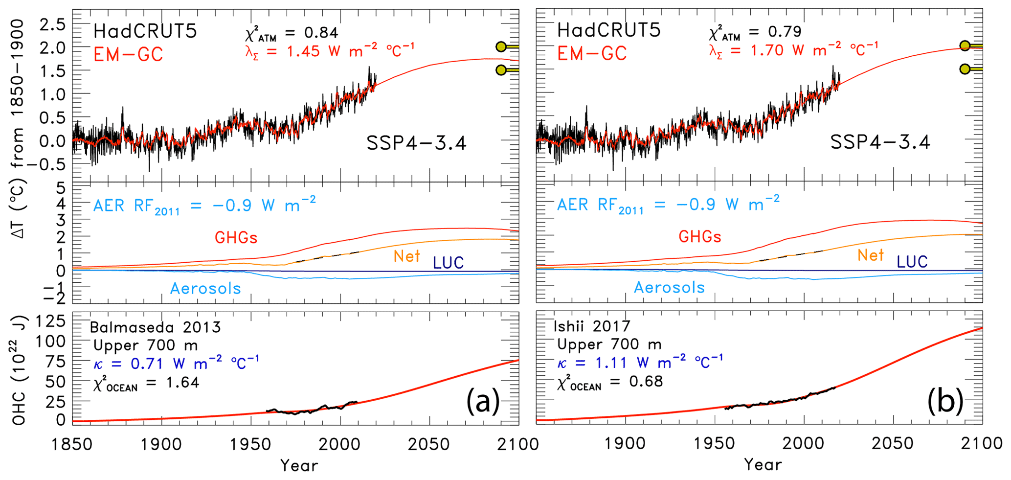
Figure 4 Measured (HadCRUT5) and EM-GC simulated GMST change (ΔT) from 1850–2019, as well as projected ΔT to the year 2100 for SSP4-3.4. The top box in each panel shows observed (black) and simulated (red) ΔT, the λ_Σ and ${\mathit{\chi }}_{\mathrm{ATM}}^{\mathrm{2}}$ values, and the Paris Agreement target and upper limit. The second row of boxes displays the contribution of GHGs, aerosols, and land-use change to ΔT. The bottom boxes compare the observed (black) and modeled (red) OHC for two different OHC records and display the value of κ needed to provide best fits to the OHC record, as well as best-fit values of ${\mathit{\chi }}_{\mathrm{OCEAN}}^{\mathrm{2}}$. Both use an aerosol RF in 2011 of −0.9 W m⁻². (a) OHC record from Balmaseda et al. (2013). (b) OHC record from Ishii et al. (2017).

2.3 Attributable anthropogenic warming rate

The attributable anthropogenic warming rate, or AAWR, is the time rate of change in GMST due to humans from 1975–2014. We use AAWR as a metric in the EM-GC framework to quantify the human influence on global warming over the past few decades and, most importantly, to also assess how well the CMIP6 GCMs can replicate this quantity. This analysis is motivated by the study of Foster and Rahmstorf (2011), who examined the human influence on the time rate of change in GMST from 1979–2010 using a residual method. We extend the end year of our analysis to 2014 because this is the last year of the CMIP6 historical simulation. We pushed the start year back to 1975 so that our analysis covers a 40-year period, over which the effect of human activity on GMST rose nearly linearly with respect to time (Figs. 1b and S10c).

We calculate AAWR utilizing the EM-GC by computing a linear fit to the ΔT_HUMAN,ATM term,

$$\begin{array}{}\text{(9)}& \begin{array}{rl}\mathrm{\Delta }{T}_{\mathrm{ATM},\mathrm{HUMAN}i}& ={\displaystyle \frac{\mathrm{1}+\mathit{\gamma }}{{\mathit{\lambda }}_p}}\left\{\mathrm{GHG}\mathrm{\Delta }{\mathrm{RF}}_i+\mathrm{AER}\mathrm{\Delta }{\mathrm{RF}}_i\right.\\ & \left.+\mathrm{LUC}\mathrm{\Delta }{\mathrm{RF}}_i-Q_{\mathrm{OCEAN}}\right\},\end{array}\end{array}$$

for a regression that spans 1850–2019. The ΔT_HUMAN,ATM term represents the net impact of the change in GMST due to RF of climate by anthropogenic GHGs, tropospheric aerosols, and the variation in surface reflectivity due to land-use change (deforestation), taking into account that for each model time step, a portion of the human-induced climate forcing is exported to the world's oceans. For each simulation, the slope of the linear least squares fit to the 480 monthly values of ΔT_HUMAN,ATM is used to determine AAWR. For the time period 1975–2014, a value for AAWR of 0.167±0.007 ^∘C per decade is found using a value of AER RF₂₀₁₁ equal to −0.9 W m⁻², wherein the uncertainty corresponds to the 2σ standard error of a linear least squares fit. The computation of AAWR found by fitting monthly values of ΔT_HUMAN,ATM is insensitive to modest changes in the start and end year for the AAWR calculation (see Table S1). The value of λ_Σ, and therefore AAWR, is also insensitive to whether or not the AMOC, PDO, or IOD terms are included in the regression framework (Canty et al., 2013; Hope et al., 2017). We are able to fit the climate record better (i.e., smaller values of χ² in Eqs. 6, 7, and 8) by including the AMOC term. However, computed values of AAWR are insensitive to whether the AMOC is used in the regression because whatever contributions the variation in the strength of the thermohaline circulation may have had on GMST are not considered in Eq. (9) (see Fig. S11 for further explanation).

The determination of AAWR from historical CMIP6 near-surface air temperature output involves conducting a regression of deseasonalized, globally averaged, monthly ΔT(ΔT^DES,GLB) from each GCM (Hope et al., 2017), termed the REG method. The archived CMIP6 historical runs are constrained by observed variations in SAOD and influenced by other factors such as internal model-generated ENSOs. The ΔT^DES,GLB time series for all of the runs from each CMIP6 GCM are averaged together to obtain one time series of ΔT^DES,GLB for each GCM. This average ΔT^DES,GLB time series is used to compute AAWR. The regression approach is used to compute the influence of SAOD on GMST from CMIP6 GCMs. The time needed for GMST to respond to a change in the aerosol loading in the stratosphere due to a volcanic eruption in each GCM can exhibit a significant difference compared to the empirically determined response time of 6 months discussed in Sect. 2.1. A lag was determined for each GCM by calculating the value of the monthly delay between volcanic eruptions and the surface temperature response that resulted in the largest regression coefficient for SAOD. We regress the ΔT^DES,GLB against SAOD and the anthropogenic effect on temperature, which is approximated as a linear function from 1975–2014. The value of AAWR is the slope of the anthropogenic effect on temperature. Figure S12 illustrates the REG method used to determine AAWR from the CMIP6 GCMs. Table S3 depicts the slight effect on values of AAWR for the CMIP6 GCMs of changing the start or end year for the regression. At the time of analysis, there are 50 CMIP6 GCMs with the necessary archived output to calculate AAWR, with the values of AAWR found using REG shown in Table S3. Figure S13 and the Supplement compare values of AAWR found using the REG method applied to EM-GC output with values of AAWR found using Eq. (9) as support for the validity of using the REG method to determine AAWR from CMIP6 output.

We also use a second method to extract the value of AAWR from the CMIP6 multi-model ensemble. This method, termed LIN, involves a linear regression of global, annual average values of GMST from the CMIP6 multi-model ensemble (Hope et al., 2017). For LIN, we exclude the years of obvious volcanic influence on the rise in GMST from the CMIP6 multi-model ensemble historical simulations: i.e., data for 1982 and 1983 (following the eruption of El Chichón) and 1991 and 1992 (following the eruption of Mount Pinatubo) are excluded. Archived global, annual average values of GMST covering 1975–2014, excluding these 4 years, are fit using linear regression, with the AAWR set equal to the slope of the fit. Values of AAWR for 1975–2014 found using LIN are also shown in Table S4 for each GCM. Analysis of AAWR for these 50 GCMs of LIN versus REG (see Fig. S14) results in a correlation coefficient (r²) of 0.995 and a mean ratio of 1.009±0.015, with LIN-based AAWR exceeding REG-based AAWR by about 1 %. The close agreement of AAWR found using both methods provides strong evidence for the accurate determination of AAWR from the CMIP6 GCMs. We use the REG method in this analysis because it provides a more rigorous technique to remove the influence of SAOD on GMST from the CMIP6 multi-model ensemble compared to the LIN method.

The CMIP6 multi-model ensemble provides simulations of near-surface air temperature (TAS), which we use to calculate AAWR. The EM-GC uses blended near-surface air temperature to determine values of AAWR. Cowtan et al. (2015) provide a method to create blended near-surface air temperature output from the GCMs. The CMIP6 multi-model ensemble contains archived fields of TAS and the temperature at the interface of the atmosphere and the upper boundary of the ocean (TOS) (Griffies et al., 2016), whereas only a subset of GCM groups provide the archived land fraction needed to calculate blended near-surface air temperature using the Cowtan et al. (2015) method. Cowtan et al. (2015) compared the modeled and measured trend in global temperature over 1975–2014 and found a 4.0 % difference in the trend upon the use of blended temperature from CMIP5 GCMs rather than global modeled TAS. Their analysis focused on a comparison of modeled and measured temperature, not just the anthropogenic component. We have used the method of Cowtan et al. (2015) to create blended CMIP6 temperature output for the CMIP6 GCMs that provide TAS, TOS, and the land fraction. Upon our use of blended CMIP6 temperature output for these GCMs and calculation of AAWR for 1975–2014, we find that AAWR based on blended CMIP6 temperature is 3.5 % lower than AAWR found when using only TAS. Tokarska et al. (2020b) estimate an effect of 0.013 ^∘C per decade in the trend of CMIP6 temperature output upon the use of blended CMIP6 temperature instead of TAS, while Cowtan et al. (2015) report a difference of 0.030 ^∘C per decade between the trend in observations and modeled output. Since the difference between values of AAWR found using blended CMIP6 temperature output and TAS is so small and does not affect any of our conclusions, we use TAS output from the CMIP6 multi-model archive because this choice allows many more GCMs to be examined.

2.4 Effective climate sensitivity

The equilibrium climate sensitivity represents the warming that would occur after the climate equilibrated with atmospheric CO₂ at the 2× pre-industrial level (Kiehl, 2007; Otto et al., 2013; Schwartz, 2012). In our model framework, we infer the climate sensitivity based on an estimate of climate feedback from the historical record, resulting in the effective climate sensitivity (ECS) (Tokarska et al., 2020a). Effective climate sensitivity is defined by IPCC 2013 as “an estimate of the global mean surface temperature response to doubled carbon dioxide concentration evaluated from model output or observations for evolving non-equilibrium conditions”. To calculate ECS from the EM-GC, we use

$$\begin{array}{}\text{(10)}& \mathrm{ECS}={\displaystyle \frac{\mathrm{1}+\mathit{\gamma }}{{\mathit{\lambda }}_{\mathrm{P}}}}\times \mathrm{5.35}\mathrm{W}{\mathrm{m}}^{-\mathrm{2}}\times \ln \left(\mathrm{2}\right),\end{array}$$

which represents the rise in GMST for a doubling of CO₂, assuming no other perturbations and equilibrium in other components of the climate system (i.e., Q_OCEAN=0) (Mascioli et al., 2012). The expression for the radiative forcing of CO₂ is from Myhre (1998). The quantity γ in Eq. (10), which represents the sensitivity of the GMST to feedbacks within the climate system, is the only variable component of ECS. We only use values of γ that result in good fits (χ²≤2 for Eq. 6 to 8) between modeled and observed GMST and modeled and observed OHC. We refer to the quantity in Eq. (10) as effective climate sensitivity, rather than equilibrium climate sensitivity, because for most of our analysis we assume a constant value of climate feedback inferred from prior observations.

For the estimate of climate sensitivity from the CMIP6 multi-model ensemble, we use the method described by Gregory et al. (2004) (see the Supplement and Fig. S15 for more information). The Gregory et al. (2004) method also estimates effective climate sensitivity from the CMIP6 GCMs (Gregory et al., 2004; Sherwood et al., 2020; Zelinka et al., 2020) because it assumes that the feedbacks inferred from the first 150 years of the abrupt 4× CO₂ CMIP6 GCM simulations persist until equilibrium. At the time of this analysis, 28 models released the necessary output to the CMIP6 archive (see Table S5 for the list of models and individual values of ECS). Several recent analyses suggest the Gregory method underestimates the true value of equilibrium climate sensitivity from the CMIP6 multi-model output (Rugenstein et al., 2020; Sherwood et al., 2020; Zelinka et al., 2020). However, effective climate sensitivity is strongly correlated with the amount of warming simulated by GCMs for high carbon emission scenarios and is more relevant for warming over the timescale of interest (rest of this century) due to the long time needed to achieve equilibrium (Sherwood et al., 2020). We use the Gregory method to calculate ECS from the CMIP6 GCMs because this procedure is preferred by Eyring et al. (2016) for use within the CMIP6 community.

The estimates of climate sensitivity from Eq. (10) and those found using the Gregory et al. (2004) method are termed “effective” because they assume that climate feedback inferred from either the historical climate record or the abrupt 4× CO₂ experiment persists until equilibrium. However, these estimates of ECS differ in that the perturbation to the RF of climate over the historical record is considerably smaller than the RF of climate that underlies the 4× CO₂ experiment of the Gregory et al. (2004) method. We quantify the impact of time-variable climate feedback on climate sensitivity in Sect. 3.3.6.

2.5 Aerosol weighting method

Probabilistic forecasts of the future rise in GMST for various SSPs are an important part of our analysis. Probabilities of AAWR and ECS are computed by considering the uncertainty in AER RF₂₀₁₁. We also provide probabilistic estimates of AAWR and ECS. All of these quantities are computed by incorporating the uncertainty in the radiative forcing of climate due to tropospheric aerosols within results of our EM-GC simulations. We use an asymmetric Gaussian to assign weights to the value of GMST, AAWR, or ECS found for various time series of radiative forcing by aerosols associated with particular values of AER RF₂₀₁₁. Figure 5a shows the asymmetric Gaussian function we use to maximize the values of AAWR or ECS at the best estimate of AER RF₂₀₁₁ of −0.9 W m⁻², accomplished by giving these values the highest weighting. The IPCC 2013 “likely” range limits of AER RF₂₀₁₁ of −0.4 and −1.5 W m⁻² (Myhre et al., 2013) are assigned to the 1σ values of the Gaussian, and the AAWR or ECS estimates occurring at the “likely” range AER RF₂₀₁₁ limits are given the same weighting. The −0.1 and −1.9 W m⁻² limits of the AER RF₂₀₁₁ range are assigned as the 2σ values of the asymmetric Gaussian based on the IPCC 2013 description of these two values as being 5 % and 95 % uncertainty limits (Myhre et al., 2013). The Gaussian we use is asymmetric due to the fact that the distribution of the likely range and the 5th and 95th percentiles of the values of AER RF₂₀₁₁ are not distributed symmetrically from the best estimate of −0.9 W m⁻². For example, the likely ranges of AER RF₂₀₁₁ are given as −0.4 and −1.5 W m⁻²; the −0.4 W m⁻² value is 0.5 W m⁻² from the best estimate, whereas −1.5 W m⁻² is 0.6 W m⁻² from the best estimate. We fit a Gaussian to the likely range and the 5th and 95th percentiles that have a slightly different shape on either side of the best estimate, as shown in Fig. 5a.

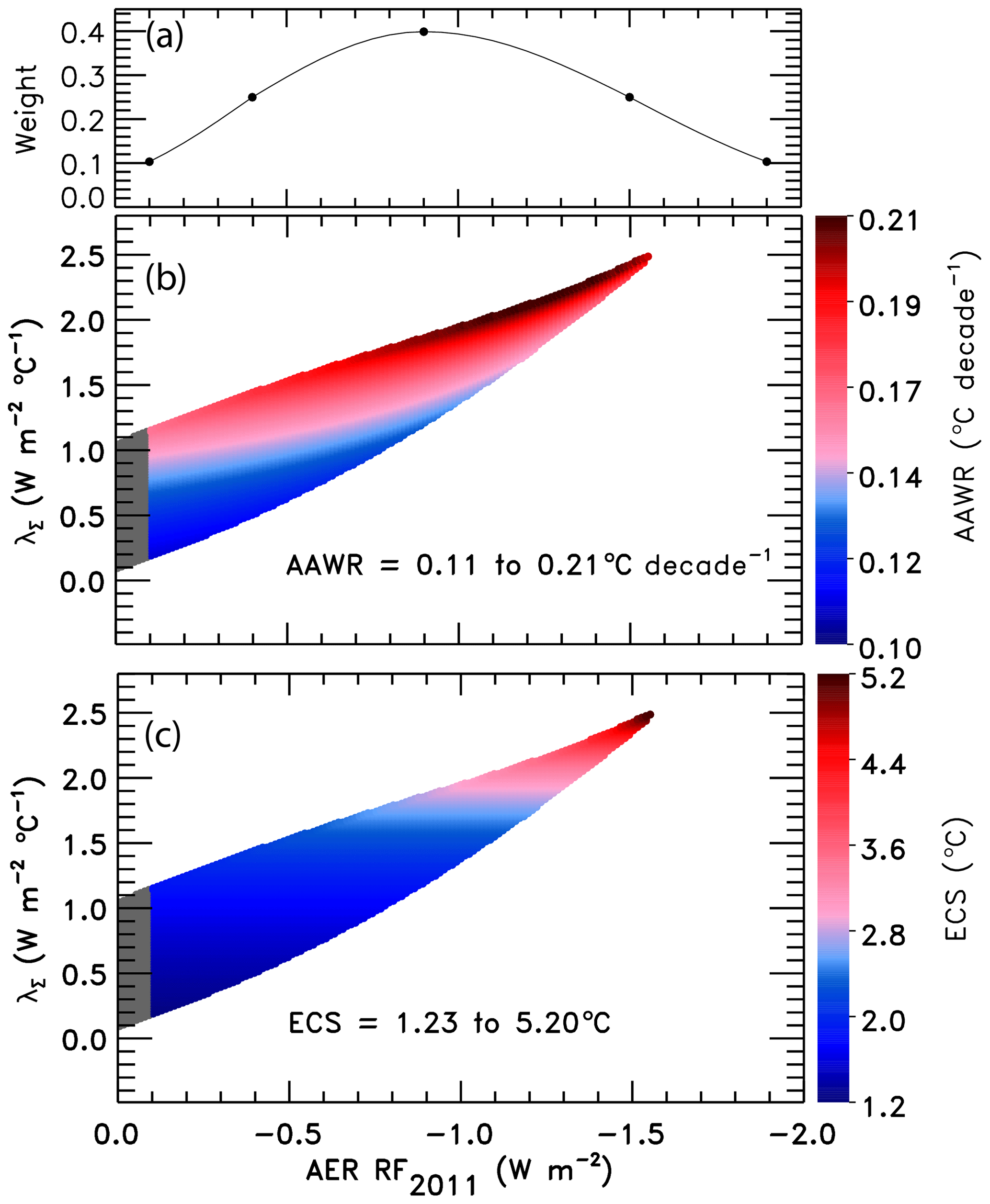
Figure 5 Aerosol weighting method. (a) The weights assigned to an asymmetric Gaussian distribution of AER RF₂₀₁₁ based on values provided by Chapter 8 of IPCC 2013. The five black circles indicate the assigned weights for the AER RF₂₀₁₁ best estimate of −0.9 W m⁻², likely range of −0.4 and −1.5 W m⁻², and the 5th and 95th confidence intervals of −0.1 and −1.9 W m⁻². (b) Values of AAWR in degrees Celsius per decade as a function of the climate feedback parameter, λ_Σ, and the value of AER RF₂₀₁₁ associated with various time series for the RF of climate due to tropospheric aerosols. The colors denote the values of AAWR calculated from 1975–2014 using the EM-GC trained with the HadCRUT5 ΔT record. (c) ECS (^∘C) as a function of λ_Σ and the value of AER RF₂₀₁₁. The colors denote values of ECS found using the EM-GC. For panels (b) and (c), model results are shown only for combinations of λ_Σ and RF due to tropospheric aerosols for which good fits to the climate record could be achieved.

Figure 5b shows the value of AAWR (^∘C per decade) as a function of the climate feedback parameter, λ_Σ, and AER RF₂₀₁₁. We are able to find more good fits to the observed GMST for small values of AER RF₂₀₁₁ than at larger values of AER RF₂₀₁₁. Therefore, we bin values of AAWR (Fig. 5b), ECS (Fig. 5c), or future GMST (described in Sect. 3.3) by AER RF₂₀₁₁ and find the probability distribution for values of AAWR, ECS, or future GMST within each bin. The resulting probability distributions are assigned the weights associated with each value of AER RF₂₀₁₁ in the bins to arrive at the probabilistic estimates of AAWR or ECS shown in Sect. 3. If we did not use this procedure and instead simply averaged all of the values for AAWR and ECS shown in Fig. 5, undue emphasis would be given to model results that occur at small AER RF₂₀₁₁ (see Fig. S16 for unweighted ECS values). This aerosol weighting method allows the expert assessment of the likely range of RF due to tropospheric aerosols given in Chapter 8 of IPCC 2013 (Myhre et al., 2013) to be quantitatively incorporated into our computations of AAWR, ECS, and GMST.

3 Results

3.1 AAWR, comparison to CMIP6 multi-model ensemble

An important measure of any climate model is the ability to accurately simulate the human influence on the global mean surface temperature (GMST) anomaly. We use the attributable anthropogenic warming rate (AAWR) found by our highly constrained Empirical Model of Global Climate (EM-GC) to quantify how well the CMIP6 multi-model ensemble (see Table S7 for a list of CMIP6 GCMs analyzed in this study) is able to simulate the human influence on global warming over the past several decades.

Figure 6 compares values of AAWR from 1975–2014 computed using our EM-GC with AAWR found utilizing archived output from the CMIP6 multi-model ensemble. Seven GMST data sets and five OHC records can be used to estimate AAWR with the EM-GC. For each choice, AAWR exhibits sensitivity to the variation of the time series of radiative forcing due to tropospheric aerosols. Each box-and-whisker plot found using our EM-GC shows, for a particular choice of GMST and OHC data record, the 25th, 50th, and 75th percentiles of AAWR (box) and the 5th and 95th percentiles (whiskers) found using the aerosol weighting method described in Sect. 2.5. The star symbol indicates the minimum and maximum values of AAWR for each value of GMST data set and OHC record. The choice of OHC record and GMST data set has a slight effect on AAWR, as shown by the colored EM-GC symbols in Fig. 6. The averages of the five 25th, 50th, and 75th percentiles of AAWR found using the HadCRUT5 data set for GMST are 0.138, 0.157, and 0.176 ^∘C per decade, respectively. The 5th and 95th percentile values of AAWR from HadCRUT5 are 0.120 and 0.195 ^∘C per decade.

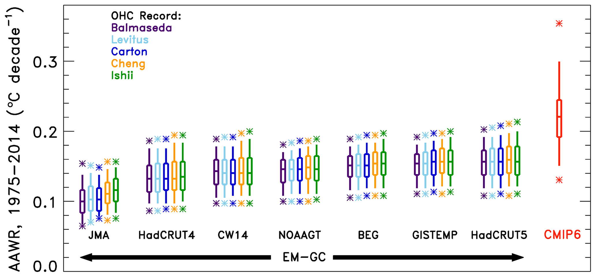
Figure 6 AAWR from the EM-GC and CMIP6 multi-model ensemble for 1975–2014. Seven temperature data sets and five ocean heat content records are used to compare values of AAWR computed from the EM-GC. The box represents the 25th, 50th, and 75th percentiles, the whiskers denote the 5th and 95th percentiles, and the stars show the minimum and maximum values of AAWR from the EM-GC based on the aerosol weighting method described in Sect. 2.5. The red box labeled “CMIP6” shows the 25th, 50th, and 75th percentiles, the whiskers represent the 5th and 95th percentiles, and the stars denote the minimum and maximum values of AAWR from the 50-member CMIP6 multi-model ensemble.

The box-and-whisker symbol labeled CMIP6 in Fig. 6 shows the 5th, 25th, 50th, 75th, and 95th percentiles of AAWR calculated from 50 GCMs, also from 1975–2014, as described in Sect. 2.3. The stars denote the minimum and maximum values of AAWR from the GCMs. Two CMIP6 models exhibit values of AAWR similar to the median values we infer from the HadCRUT4, CW14, NOAAGT, BEG, GISTEMP, and HadCRUT5 data records using the EM-GC. In particular, INM-CM5-0 (Volodin and Gritsun, 2018) yields 0.147 ^∘C per decade and MIROC6 (Tatebe et al., 2019) results in 0.157 ^∘C per decade (Table S4 provides values of AAWR for all individual CMIP6 GCMs). The median value of AAWR from the CMIP6 multi-model ensemble is 0.221 ^∘C per decade, about 40 % larger than the 50th percentile value of AAWR found using the HadCRUT5 data set for GMST. The 5th, 25th, 75th, and 95th percentiles of AAWR from the CMIP6 multi-model ensemble are 0.151, 0.192, 0.245, and 0.299 ^∘C per decade, respectively. Some CMIP6 GCMs exhibit values of AAWR that are 0.14 ^∘C per decade larger than our largest empirical estimates for 1975–2014; the maximum value of AAWR from the GCMs is 0.354 ^∘C per decade. The maximum value of AAWR based on the historical climate record using the EM-GC is 0.213 ^∘C per decade (HadCRUT5 data set using the Ishii et al., 2017, OHC record and a time series for RF due to tropospheric aerosols consistent with AER RF₂₀₁₁ equal to −1.5 W m⁻²). All of the EM-GC-based values of AAWR in Fig. 6 are below the 50th percentile of AAWR from the CMIP6 multi-model ensemble of 0.221 ^∘C per decade, supporting the notion that CMIP6 GCMs tend to exhibit a faster rate of anthropogenic warming over the past 4 decades than the actual atmosphere.

Our determination that the rate of global warming from the CMIP6 multi-model ensemble over the time period 1975–2014 significantly exceeds the rise in GMST attributed to human activity is aligned with a similar finding highlighted in Fig. 11.25b from Chapter 11 of the IPCC 2013 report that CMIP5 models tend to warm too quickly compared to the actual climate system over the time period 1975–2014 (Kirtman et al., 2013). The values of AAWR from the CMIP6 multi-model ensemble from our analysis present a similar finding as Tokarska et al. (2020b) and CONSTRAIN (2020) that some of the CMIP6 models overestimate recent warming trends. Tokarska et al. (2020b) examine the trend in the human component of GMST from 1981–2014. We arrive at a similar conclusion as these studies that CMIP6 GCMs overestimate the rate of global warming for the 1982–2014 time period of AAWR as shown in Tables S2 and S3. Our results, the finding by the IPCC 2013 report, Tokarska et al. (2020b), and CONSTRAIN (2020) appear to be quite different than the conclusion of Hausfather et al. (2020) that past climate models have matched recent temperature observations quite well. The Hausfather et al. (2020) study does not examine CMIP5 GCMs, let alone CMIP6 GCMs, and the last two rows of their Table 1 indicate that the skill of climate models forecasting the change in GMST over time decreased considerably between the Third Assessment Report (TAR) and the Fourth Assessment Report (AR4). The change in temperature over time for the TAR and AR4 only spans 17 and 10 years, respectively (Hausfather et al., 2020). In Fig. 6, we examine the ability of the GCMs to simulate the rise in GMST attributed to humans over a 40-year time period, which provides a better measure of how well the models simulate the observations than the shorter time period. The temperature change over time for the TAR and AR4 examined by Hausfather et al. (2020) ends in 2017, which was right after a very strong ENSO, so their analysis may be influenced by the 2015 to 2016 ENSO event. In contrast, our analysis of AAWR is not influenced by natural variability such as ENSO because we examine the human component of global warming after explicitly accounting for and removing the influence of ENSO on GMST. Consequently, our determination of AAWR from observations (Table S2) and GCMs (Table S3) depends only to a small extent on the specification of the start year (for values ranging from 1970 to 1984) and end year (2004 to 2018). Our analysis shows that upon quantification of the human driver of global warming within both the data record and climate models, the CMIP6 GCMs warm faster than observed GMST over the past 4 decades regardless of precise specification of the start and end year.

3.2 ECS

Climate sensitivity is a metric often used to compare the sensitivity of warming among GCMs and with warming inferred from the historical climate record. Figure 7 shows values of effective climate sensitivity (ECS) inferred from the climate record using our EM-GC, seven GMST data sets, and five OHC records. As for AAWR, the largest variation in ECS is driven by uncertainty in AER RF₂₀₁₁. The colored circles represent the ECS values found using the IPCC 2013 best estimate of AER RF₂₀₁₁ of −0.9 W m⁻² (Myhre et al., 2013). The ECS values found utilizing the EM-GC are displayed using a box-and-whisker symbol. The middle line represents the median values of ECS, and the box is bounded by the 25th and 75th percentiles. The whiskers connect to the 5th and 95th percentiles, and the stars denote the minimum and maximum values. We use the aerosol weighting method described in Sect. 2.5 to calculate the percentiles for ECS; values of ECS found without aerosol weighting are shown in Fig. S16. Varying the choice of GMST data record has a slight effect on the value of ECS, whereas the choice of OHC record has a larger effect, as indicated by the various heights of the boxes and whiskers and the maximum values of ECS. In the EM-GC framework, the ocean heat export term (Q_OCEAN) represents disequilibrium in the climate system. We compute values of Q_OCEAN from various records of OHC. If the current value of Q_OCEAN is as large as suggested by the Cheng 2017 and Ishii et al. (2017) OHC records, then Earth's climate will exhibit a larger rise in GMST to reach equilibrium than if the value of Q_OCEAN inferred from the OHC record of Balmaseda et al. (2013) is correct. The averages of the 25th, 50th, and 75th percentiles of ECS found using the HadCRUT5 data set for GMST are 1.74, 2.12, and 2.67 ^∘C, respectively. The average best estimate of ECS using the HadCRUT5 data set and an AER RF₂₀₁₁ value of −0.9 W m⁻² is 2.33 ^∘C.

Figure 7 ECS from the EM-GC and the CMIP6 multi-model ensemble. Seven GMST data sets and five ocean heat content records are used to compare values of ECS computed from the EM-GC. The box represents the 25th, 50th, and 75th percentiles, the whiskers denote the 5th and 95th percentiles, and the stars indicate the minimum and maximum values of ECS using the EM-GC based on the weighting method described in Sect. 2.5. The circles denote the value of ECS associated with the best estimate of AER RF₂₀₁₁ of −0.9 W m⁻². The red box labeled “CMIP6” represents the 25th, 50th, and 75th percentiles, the whiskers denote the 5th and 95th percentiles, and the stars indicate the minimum and maximum values of ECS from the 28-member CMIP6 multi-model ensemble.

The box-and-whisker symbol labeled CMIP6 in Fig. 7 shows the 25th, 50th, 75th, and 5th and 95th percentiles of ECS calculated from the output of 28 CMIP6 models, as described in Sect. 2.4. Minimum and maximum values are represented by stars. The values of ECS from the CMIP6 multi-model ensemble are larger than the majority of values inferred from the climate record using the EM-GC. The height of the box for the CMIP6 multi-model ensemble estimate of ECS is larger than the height of the boxes for ECS inferred from the climate record using the EM-GC, indicating that the GCMs exhibit a wide range of ECS values. The 25th and 75th percentiles of ECS from the CMIP6 multi-model ensemble are 2.84 and 4.93 ^∘C, respectively. The 5th percentile of ECS from the CMIP6 multi-model ensemble is 2.19 ^∘C, and the 95th percentile is 5.65 ^∘C (see Table S4 for ECS values for specific models). In contrast, the average 5th and 95th percentiles from the EM-GC are 1.40 and 3.57 ^∘C, respectively. The median value of ECS from the CMIP6 multi-model ensemble is 3.74 ^∘C, which is 1.6 times the best estimate of 2.33 ^∘C found using the HadCRUT5 temperature record. All estimates of ECS described above are found assuming constant climate feedback over time. If climate feedback changes over time, then our estimates of ECS will increase as discussed in Sect. 3.3.6.

Figure 8 summarizes values of ECS found utilizing the analysis of the century-and-a-half-long climate record using our EM-GC, our examination of a 28-member CMIP6 GCM ensemble, and 13 other recent studies. The studies are divided into three categories: those that estimated ECS based on observations (historical analysis), others that used GCM output but constrained the output in some way (Constrained GCM output), and studies that examined raw GCM output (GCM output). We obtain a best estimate for ECS of 2.33 ^∘C using the HadCRUT5 data record and a value of AER RF${}_{\mathrm{2011}}=-\mathrm{0.9}$ W m⁻² with a range of ECS of 1.40–3.57 ^∘C (5th and 95th percentile confidence interval). The use of HadCRUT5 rather than HadCRUT4 induces a significant rise in our best estimate of ECS, which is 1.99 ^∘C (range of 1.12–3.63 ^∘C) upon use of HadCRUT4. Both of these estimates of ECS largely fall within the range provided by IPCC 2013 of 1.5 to 4.5 ^∘C for ECS and is supported by four other derivations of ECS from the empirical climate record: 2.0 ^∘C (range of 1.2–3.9 ^∘C) given by Otto et al. (2013), 1.87 ^∘C (range of 1.1–4.05 ^∘C) given by Lewis and Grünwald (2018), 2.0 ^∘C (range of 1.3–3.1 ^∘C) given by Tokarska et al. (2020a), and 2.0 ^∘C (range of 1.2–3.1 ^∘C) given by Skeie et al. (2018) (all range values are for the 5th and 95th percentile confidence interval). All of these studies preceded the release of HadCRUT5. Our estimate of ECS covers a similar range of values as given by Cox et al. (2018), Dessler et al. (2018), and Nijsse et al. (2020), as illustrated in Fig. 8. Our determination of ECS from the CMIP6 GCMs resembles that from Proistosescu and Huybers (2017) and Zelinka et al. (2020), as indicated in the “GCM output” category in Fig. 8.

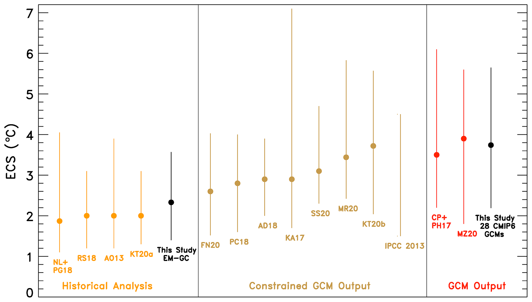
Figure 8 Values of ECS from the EM-GC (black) trained using the HadCRUT5 GMST record, our analysis of the CMIP6 multi-model ensemble (black), and 13 other studies grouped by type of analysis. The studies are listed by lead author (first initial of their first name and first initial of their last name) and the year of publication unless there are only two authors, in which case the initials of both authors are listed. The historical analysis includes Lewis and Grünwald (2018) NL+PG18, Otto et al. (2013) AO13, Skeie et al. (2018) RS18, and Tokarska et al. (2020a) KT20a. Constrained GCM output includes Armour (2017) KA17, Cox et al. (2018) PC18, Dessler et al. (2018) AD18, Nijsse et al. (2020) FN20, Rugenstein et al. (2020) MR20, Sherwood et al. (2020) SS20, Stocker et al. (2013) IPCC 2013, and Tokarska et al. (2020b) KT20b. GCM output includes Proistosescu and Huybers (2017) CP+PH17 and Zelinka et al. (2020) MZ20. The studies estimating effective climate sensitivity are AO13, NL+PG18, RS18, FN20, SS20 KT20a, KT20b, and MZ20. The studies estimating equilibrium climate sensitivity are KA17, AD18, PC18, MR20, and CP+PH17. See the Supplement for the confidence intervals shown for each study and more information about which studies estimate effective or equilibrium climate sensitivity.

Recent studies have shown that the CMIP6 multi-model ensemble exhibits higher values of ECS than the CMIP5 models because of larger, positive cloud feedbacks within the latest models (Gettelman et al., 2019; Meehl et al., 2020; Sherwood et al., 2020; Zelinka et al., 2020). The IPCC 2013 report gives a likely range of 1.5 ^∘C to 4.5 ^∘C for climate sensitivity (Stocker et al., 2013), and some of the CMIP6 GCMs analyzed in this study have values of ECS more than 1 ^∘C above this range. However, some in the climate community seem to currently doubt whether the very large values of ECS are representative of the real world (CONSTRAIN, 2020; Forster et al., 2020; Lewis and Curry, 2018; Tokarska et al., 2020b). Gettelman et al. (2019) found that the newest version of the Community Earth System Model (CESM2) has a higher value of ECS than CESM1 (5.3 ^∘C versus 4.0 ^∘C) and urge the climate community to work together to determine the plausibility of such high values of ECS. Zhu et al. (2020) found that the high values of ECS in CESM2 and other GCMs is not supported by the paleoclimate record and are biased too warm. An analysis by Nijsse et al. (2020) coupled the CMIP6 multi-model ensemble to a two-box energy balance model and the climate record and obtained a median value of ECS of 2.6 ^∘C and range of 1.52–4.03 ^∘C (5th and 95th percentiles). Similarly, Sherwood et al. (2020) conclude that cooling during the Last Glacial Maximum provides strong evidence against ECS being greater than 4.5 ^∘C and conclude that ECS lies within the range of 2.3 to 4.7 ^∘C at the 5th to 95th percentile confidence intervals.

We obtain a wide range of ECS values from our EM-GC simulations of the climate record due to consideration of the uncertainty in the radiative forcing of climate from tropospheric aerosols (Figs. 5c and 7). However, under one circumstance, we find values of ECS using the EM-GC that are similar to the maximum value of ECS from the CMIP6 multi-model ensemble. Our large estimate of ECS occurs if we assume that anthropogenic aerosols have exhibited strong cooling and offset a large amount of greenhouse gas warming such that the observed GMST record can only be well simulated under the condition of large climate feedback (i.e., values of λ_Σ in Eq. 3 greater than or equal to 2.45 W m^−2 ∘C⁻¹). If aerosols have truly strongly cooled the climate, offsetting the vast majority of the rise in RF due to greenhouse gases as suggested by Shen et al. (2020), the actual value of ECS may lie close to 5 ^∘C or larger. Under the scenario that aerosols have not cooled this strongly (Bond et al., 2013), then it is feasible that ECS lies well below 5 ^∘C. The highest values of ECS found using our analysis (red portion of Fig. 5c) are assigned low weights due to the assessment by Myhre et al. (2013) that the large AER RF₂₀₁₁ associated with these ECS values is unlikely.

Five empirical determinations of ECS (our study plus Lewis and Grünwald, 2018; Otto et al., 2013; Skeie et al., 2018; and Tokarska et al., 2020a) and the CMIP5- or CMIP6-constrained estimates of Cox et al. (2018), Dessler et al. (2018), and Nijsse et al. (2020) are in slight contrast with the 2.3–4.7 ^∘C range for ECS (5th and 95th confidence interval) published recently by Sherwood et al. (2020) (Fig. 8). As noted above, Sherwood et al. (2020) use paleoclimate data to rule out the high range of ECS. They rely on a determination that the feedback due to clouds is moderately to strongly positive to rule out the low range of ECS found by our analysis and the studies noted above. We caution that knowledge of the cloud feedback from observations is generally limited to databases such as the International Satellite Cloud Climatology Project (ISCCP) (Schiffer and Rossow, 1983) and Pathfinder Atmospheres Extended (PATMOS-x) (Foster and Heidinger, 2013). While these databases are monumental in terms of complexity and scope, they cover only a fairly short (i.e., about 36 years) part of the century-and-a-half climate record (Klein et al., 2017; Sherwood et al., 2020). Most assessments of total cloud feedback rely on some combination of observations such as ISCCP, PATMOS-x, or other satellite records together with the results of regression analysis, GCM projections, and large eddy simulations that are able to resolve some of the convective processes involved in cloud formation (Klein et al., 2017; Sherwood et al., 2020). The most important component of the global cloud feedback is tropical low clouds, which Sherwood et al. (2020) consider to exert a positive feedback on climate based largely on the results of Klein et al. (2017). The determination by Klein et al. (2017) of a likely positive feedback for tropical low-altitude clouds is based on the mean and standard deviation of the central value of this feedback determined by five studies, even though four of these studies exhibit uncertainties that encompass zero feedback and the fifth nearly reaches zero (their Fig. 3). This fact, combined with the recent study by Weaver et al. (2020), who report no long-term statistically significant trend in global cloud reflectivity at 340 nm averaged between 45^∘ S and 45^∘ N based on analysis of data collected by a variety of NOAA and NASA satellite instruments, causes us to suggest that the true value of ECS may lie below the 2.3 ^∘C lower limit given by Sherwood et al. (2020).

In our model framework, the largest uncertainty in ECS is driven by imprecise knowledge of the radiative forcing of climate by tropospheric aerosols. As shown in Fig. 5c, a wide range of ECS values can be inferred from the century-and-a-half-long climate record. We stress that each value of ECS shown in Fig. 5c is based on a simulation for which ${\mathit{\chi }}_{\mathrm{ATM}}^{\mathrm{2}}$, ${\mathit{\chi }}_{\mathrm{RECENT}}^{\mathrm{2}}$, and ${\mathit{\chi }}_{\mathrm{OCEAN}}^{\mathrm{2}}$ are all less than or equal to 2. Better knowledge of AER RF for the contemporary atmosphere would lead to a reduction in the uncertainty of ECS. Numerous studies of the climate record, including our century-and-a-half simulations, infer the possibility of lower values of ECS than given by a recent analysis of studies that involve examination of data from compendiums such as ISCCP and PATMOS-x (Sherwood et al., 2020). However, the analysis by Sherwood et al. (2020) did not examine the consistency of the inferred value of ECS with the ability of models to accurately simulate the GMST anomaly between 1850 and the present or over the past 40 years.

We conclude this section by commenting on the relationship between ECS and AAWR in our model framework. Eight of the CMIP6 GCMs (GFDL-ESM4, GISS-E2-1-G, INM-CM5-0, INM-CM4-8, MIROC6, MIROC-ES2L, NorESM2-LM, and NorESM2-MM) exhibit values of ECS and AAWR consistent with the minimum and maximum estimates based on our EM-GC constrained by the HadCRUT5 GMST record (Table S5 and Fig. S17). An analysis of the relationship between AAWR and ECS from the CMIP6 GCMs illustrates that 78 % of the variance in ECS among the 28 CMIP6 GCMs that provide both quantities is explained by AAWR (see Fig. S17). This result indicates that CMIP6 GCMs that accurately simulate the rise in observed ΔT over the past few decades exhibit values of ECS that are in line with our empirically based estimate.

3.3 Future projections

3.3.1 CMIP6

The CMIP6 multi-model archive provides future projections of the GMST anomaly relative to pre-industrial (ΔT) using the ScenarioMIP Shared Socioeconomic Pathways (SSPs). Figure 9 shows the CMIP6 multi-model ensemble projections of ΔT for the four SSPs (SSP1-1.9, SSP1-2.6, SSP4-3.4, and SSP2-4.5) highlighted in our analysis. Each SSP scenario has varying numbers of gridded, monthly mean TAS projections submitted to the CMIP6 archive by GCMs. The global monthly ΔT time series for all of the runs for each CMIP6 GCM were averaged together to obtain one time series of ΔT. The varying amount of GCM output available for each SSP scenario is due to the fact that (a) SSP1-2.6 and SSP2-4.5 are Tier 1 scenarios (O'Neill et al., 2016) and are designated as priority over the other SSPs (as described in Sect. 2.2.2), and (b) not all GCMs have provided results to the CMIP6 archive at the time of the analysis. More CMIP6 multi-model output will likely become available as modeling groups who have not submitted output to the CMIP6 archive finalize their results. However, we do not expect that additional GCM simulations will affect our conclusions unless the GCM output is significantly different than that currently available.

Figure 9 Historical simulations and future projections of GMST from the CMIP6 multi-model ensemble for several SSP scenarios. (a) GCM simulations from the historical experiment and future model projections from SSP1-1.9. Observations (black) are from HadCRUT5 to the end of 2019. The IPCC 2013 likely range of warming (red) is from Fig. 11.25b in Chapter 11 of the IPCC 2013 report. The CMIP6 multi-model mean (thick, blue) and minimum and maximum (dashed, blue) lines are shown. Global monthly ΔT was created by averaging the TAS output over the globe with a cosine latitude weighting. The Paris Agreement target of 1.5 ^∘C and upper limit (yellow) of 2.0 ^∘C are included to demonstrate how the GCM projections compare. (b) Future GMST projections from SSP1-2.6. (c) Future GMST projections from SSP4-3.4. (d) Future GMST projections from SSP2-4.5.

The red trapezoid in Fig. 9 labeled as the IPCC 2013 likely range is the same trapezoid as that displayed in Fig. 11.25b from Chapter 11 of the IPCC 2013 report (Kirtman et al., 2013). The recent observations of ΔT from HadCRUT5 lie towards the top of the likely range of warming designated by this trapezoid. Many of the projections of the rise in ΔT from the CMIP6 multi-model ensemble lie above the IPCC 2013 likely range of warming. The Paris Agreement target of 1.5 ^∘C and upper limit of 2.0 ^∘C are shown as yellow circles, which are included to allow for comparison of the future projections of ΔT from the CMIP6 multi-model ensemble with the goals of the agreement. The thick blue line in each plot is the CMIP6 multi-model mean of ΔT, and the dashed blue lines are the minimum and maximum ΔT projections from the CMIP6 multi-model ensemble. For SSP1-1.9, the multi-model mean projection of ΔT in 2100 from the CMIP6 GCMs lies just above the Paris Agreement target at 1.6 ^∘C, whereas for SSP1-2.6 the CMIP6 multi-model mean reaches the Paris Agreement upper limit of 2.0 ^∘C at the end of this century. For both SSP4-3.4 and SSP2-4.5, the end-of-century CMIP6 multi-model mean lies above the Paris Agreement upper limit at 3.0 and 3.1 ^∘C, respectively.

Figure 9 illustrates that there are two groups of CMIP6 multi-model projections of ΔT, with a few GCMs having future values of ΔT that are considerably higher than others. This divergence for GCM projections of ΔT is especially evident in Fig. 9a, c, and d. The two CMIP6 GCMs that have the highest values of ΔT across the four SSPs are CanESM5 (Swart et al., 2019) and UKESM1 (Sellar et al., 2020). The CanESM5 and UKESM1 GCMs have the highest values of AAWR (0.354 and 0.299 ^∘C per decade, respectively), large values of ECS (5.70 and 5.40 ^∘C, respectively), and exceed observed ΔT reported by HadCRUT5 for the past few decades.

3.3.2 EM-GC

The EM-GC is also used to project future changes in ΔT using the SSPs. Figure 10 shows the GMST anomaly in 2100 from pre-industrial (ΔT₂₁₀₀) as a function of the climate feedback parameter and AER RF₂₀₁₁ for the four SSPs highlighted throughout. Only model runs from the EM-GC that achieved a good fit to the climate record (${\mathit{\chi }}_{\mathrm{ATM}}^{\mathrm{2}}\le \mathrm{2}$, ${\mathit{\chi }}_{\mathrm{RECENT}}^{\mathrm{2}}\le \mathrm{2}$, ${\mathit{\chi }}_{\mathrm{OCEAN}}^{\mathrm{2}}\le \mathrm{2}$) are shown. The EM-GC runs that satisfy these three χ² constraints but fall outside the IPCC 2013 range for AER RF₂₀₁₁ (Myhre et al., 2013) are shaded grey (left-hand side of each panel). We do not consider the EM-GC projections that lie outside the IPCC 2013 range for AER RF₂₀₁₁ in our projections of ΔT, yet these results are shown to illustrate that the EM-GC can fit the climate record with estimates of the RF due to tropospheric aerosols that lie below (i.e., less cooling) the 5th confidence interval of −0.1 W m⁻² for AER RF₂₀₁₁ given by IPCC 2013. We cannot establish any good fits of the HadCRUT5 GMST record for AER RF₂₀₁₁ with a cooling stronger than about −1.55 W m⁻². The ranges of ΔT₂₁₀₀ we compute using the EM-GC for SSP1-1.9, SSP1-2.6, SSP4-3.4, and SSP2-4.5 are 0.75–2.06, 0.96–2.58, 1.18–3.01, and 1.45–3.47 ^∘C, respectively. Results for SSP4-6.0, SSP3-7.0, and SSP5-8.5 are shown in Fig. S18: ΔT₂₁₀₀ ranges are 1.70–4.02, 2.26–4.93, and 2.62–6.02 ^∘C for these three scenarios.

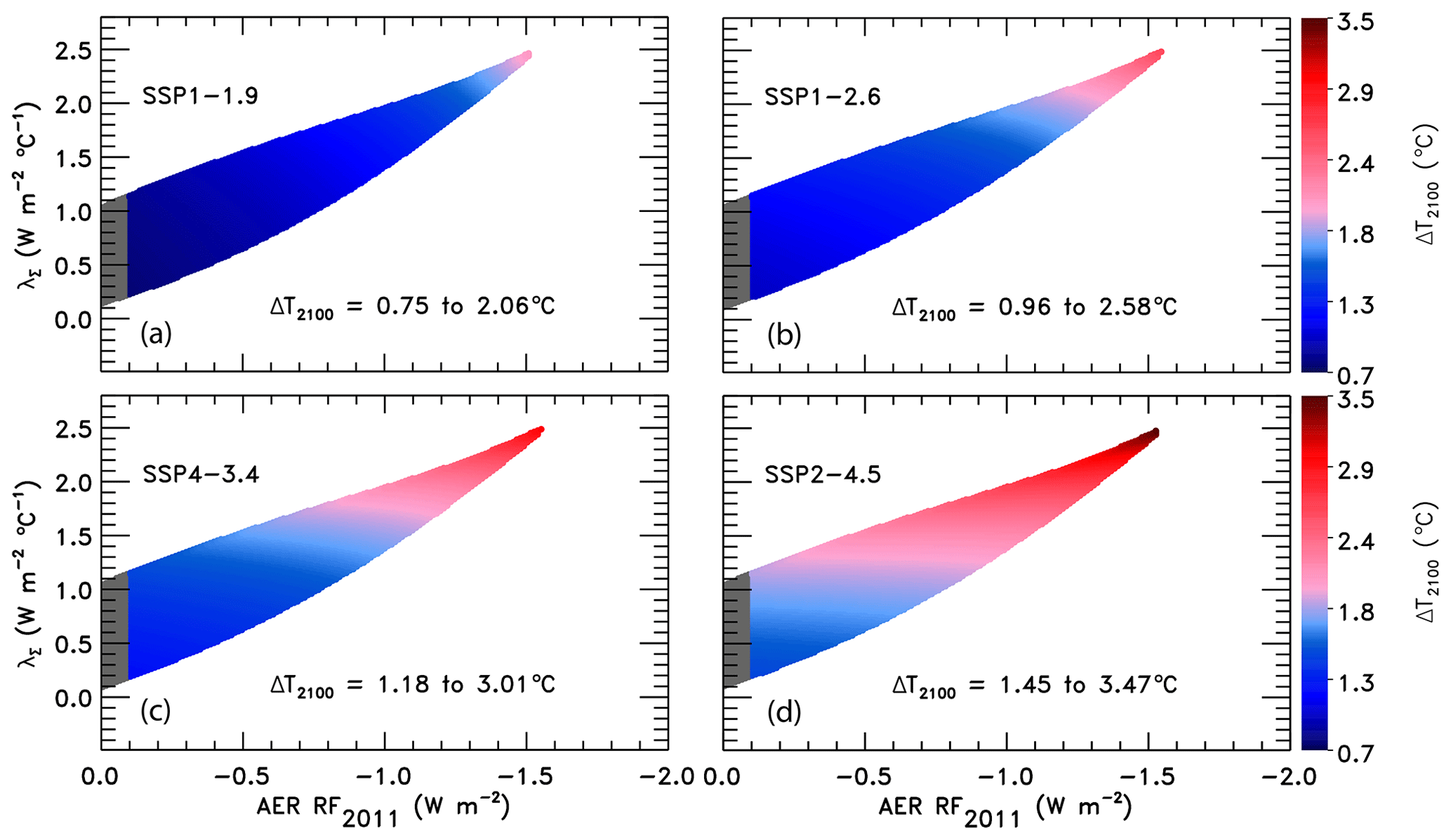
Figure 10 ΔT₂₁₀₀ as a function of climate feedback parameter and tropospheric aerosol radiative forcing in 2011 using the EM-GC trained with the HadCRUT5 ΔT record. (a) Future GMST change for SSP1-1.9. The region outside the AER RF₂₀₁₁ range provided by IPCC 2013 is shaded (grey). Colors denote the GMST change in the year 2100 relative to pre-industrial. The color bar is the same across all four panels for comparison. (b) GMST anomaly for SSP1-2.6. (c) Future temperature change for SSP4-3.4. (d) GMST anomaly for SSP2-4.5.

The large range of ΔT₂₁₀₀ found for any given SSP scenario is caused by the fact that the climate record can be fit nearly equally well by a considerably large combination of the climate feedback parameter (our λ_Σ) and scenarios for radiative forcing due to tropospheric aerosols. The more aerosols have cooled, offsetting the relatively well-known warming due to GHGs, the larger λ_Σ must be to fit the climate record. Since the RF of aerosols is set to diminish in the future due largely to public health concerns (Lelieveld et al., 2015; Shindell et al., 2016; Smith and Bond, 2014), the part of our model ensemble requiring relatively large values of λ_Σ to achieve a good fit to the climate record will result in higher values of ΔT₂₁₀₀ than other members of our model ensemble with small values of λ_Σ. Most GCMs sample only a small portion of the possible combinations of λ_Σ and AER RF₂₀₁₁ shown in Figs. 10 and S18.

3.3.3 Comparing CMIP6 and EM-GC

Time series of future projections of ΔT from the EM-GC can be illustrated as probabilistic forecasts. Figure 11 shows the change in future ΔT for SSP1-1.9, SSP1-2.6, SSP4-3.4, and SSP2-4.5 colored by the probability of reaching at least that rise in ΔT by the end of the century. The EM-GC probabilities are computed from ensemble members for model runs constrained by the HadCRUT5 data records for GMST and the average of five OHC data records (Fig. S9) based on the aerosol weighting method, as described in Sect. 2.5. The trapezoid from Chapter 11 of IPCC 2013 (Kirtman et al., 2013) is shown in Fig. 11 in black to highlight that the EM-GC projections of the future rise in ΔT lie within the IPCC 2013 likely range of warming. The Paris Agreement target and upper limit are included to compare the EM-GC projections of future ΔT to the Paris Agreement goals. The white shaded region is the EM-GC's median estimate of future ΔT for each SSP scenario. The median estimate for ΔT₂₁₀₀ for simulations using SSP1-1.9 and SSP1-2.6 falls below the Paris Agreement target at 1.1 and 1.4 ^∘C, respectively. The median estimate of ΔT₂₁₀₀ from the EM-GC for SSP4-3.4 is between the Paris Agreement target and upper limit at 1.8 ^∘C. For SSP2-4.5 the median estimate of ΔT₂₁₀₀ is 2.1 ^∘C, which is just above the Paris Agreement upper limit. The CMIP6 minimum, multi-model mean, and maximum projections of ΔT based on the ensembles in Fig. 9 are also shown in Fig. 11. The CMIP6 minimum projection of the rise in ΔT falls near the EM-GC median estimate of ΔT for each SSP scenario. The CMIP6 multi-model mean value of the future change in ΔT falls below the EM-GC maximum value of ΔT, while the CMIP6 maximum value is far above the maximum projections of the future rise in ΔT using the EM-GC. Results for SSP4-6.0, SSP3-7.0, and SSP5-8.5 are provided in Fig. S19.

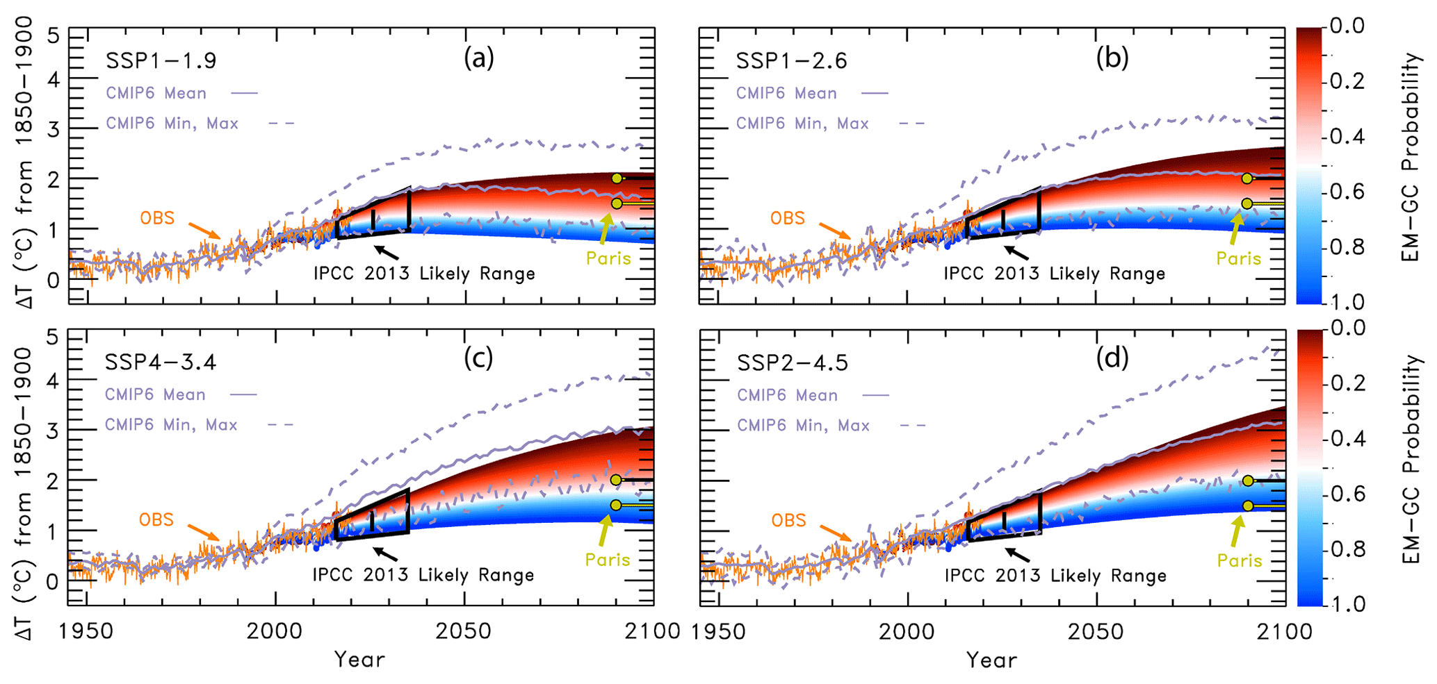
Figure 11 Probabilistic forecasts of the future rise in ΔT from the EM-GC trained using the HadCRUT5 ΔT record for several SSPs. (a) Future projections of ΔT for SSP1-1.9. Observations (orange) are from HadCRUT5. The IPCC 2013 likely range of warming (black) is from Fig. 11.25b of Chapter 11 of IPCC 2013. The Paris Agreement target and upper limit (yellow) are shown for comparison to EM-GC projections. The CMIP6 minimum, multi-model mean, and maximum values of ΔT are shown to compare to EM-GC projections. Colors denote the probability of reaching at least that temperature by the end of the century. (b) Future projections of ΔT for SSP1-2.6. (c) Future projections of ΔT for SSP4-3.4. (d) Future projections of ΔT for SSP2-4.5.

Figure 12 compares probability distribution functions (PDFs) for the projection of ΔT₂₁₀₀ utilizing the EM-GC with the HadCRUT5 GMST record and the average of the five OHC data sets and the CMIP6 multi-model ensemble. For the CMIP6 multi-model results, we compute the probabilities of achieving the Paris Agreement target of 1.5 ^∘C and upper limit of 2.0 ^∘C (at the end of the century) by calculating how many of the GCMs participating in each scenario have projections of ΔT₂₁₀₀ below the target or upper limit. The probabilities for the projections of ΔT₂₁₀₀ using the EM-GC are computed using the aerosol weighting method, as described in Sect. 2.5. The height of each histogram represents the probability that a particular range of ΔT₂₁₀₀, defined by the width of each line segment, will occur. The left-hand y axis displays the probability of ΔT₂₁₀₀ using the EM-GC, while the right-hand y axis represents the probability of ΔT₂₁₀₀ using the CMIP6 multi-model simulations. The values on the CMIP6 multi-model ensemble y axis are double the values on the EM-GC y axis for visual comparison. The solid black line denotes the Paris Agreement target, and the dotted black line signifies the upper limit in each panel. The PDFs for SSP4-6.0, SSP3-7.0, and SSP5-8.5 are shown in Fig. S20.

Figure 12 Probability density functions (PDFs) for ΔT₂₁₀₀ found using the EM-GC trained with the HadCRUT5 temperature record (dark blue) and CMIP6 multi-model results (red). (a) PDF for EM-GC results and CMIP6 multi-model results for SSP1-1.9. The left-hand y axis is for EM-GC probabilities, and the right-hand y axis is for the CMIP6 multi-model ensemble probabilities. (b) PDF for SSP1-2.6. (c) PDF for SSP4-3.4. (d) PDF for SSP2-4.5.

Numerical values of probabilities for staying at or below the Paris Agreement target for SSP1-2.6 or upper limit for SSP4-3.4 are given for the seven GMST records using the EM-GC and CMIP6 multi-model ensemble in Table 1. Projections of ΔT₂₁₀₀ based on the EM-GC provide more optimism for achieving the Paris Agreement goals than the CMIP6 multi-model ensemble regardless of which GMST data record is used. For simulations constrained using the HadCRUT5 record, the SSP1-2.6 scenario provides a 53 % (Table 1) likelihood of ΔT₂₁₀₀ staying at or below 1.5 ^∘C, and SSP4-3.4 results in a 64 % likelihood of limiting warming to 2.0 ^∘C by the end of the century. The probability of achieving the Paris Agreement target or upper limit increases upon using HadCRUT4 rather than HadCRUT5 in the EM-GC framework. The probability of achieving the 1.5 ^∘C target for SSP1-2.6 and 2.0 ^∘C upper limit for SSP4-3.4 using the HadCRUT4 GMST record is 64 % and 74 %, respectively (Table 1). This decline in attainment of the goals of the Paris Agreement upon use of HadCRUT5 reflects more rapid warming of this data record compared to HadCRUT4 (Fig. S4e versus c). The rapid warming in HadCRUT5 is driven by more accurate buoy records for SST and a statistical gap-filling procedure to attain global coverage (Morice et al., 2021). The impact on the likelihood of achieving the Paris Agreement goals for the other SSP scenarios upon using the HadCRUT4 or HadCRUT5 data records is detailed in Table S6.

An analysis by Tokarska et al. (2020b) supports our finding of a higher likelihood of attaining the goals of the Paris Agreement than suggested by the CMIP6 multi-model ensemble. Tokarska et al. (2020b) filter the CMIP6 multi-model output on the level of agreement with observations to show that the SSP1-2.6 scenario has a likely range of warming of 1.33–1.99 ^∘C above pre-industrial by the end of the century. Previous studies have suggested that a 2.6 W m⁻² scenario is in line with the 2.0 ^∘C goal (Kriegler et al., 2014, 2015; O'Neill et al., 2016; Riahi et al., 2015). Our analysis suggests that the 2.6 W m⁻² scenario provides a 86 %–98 % probability of limiting warming to 2.0 ^∘C and a 53 %–78 % probability of achieving the more stringent 1.5 ^∘C target, depending on the GMST record (Table 1). If GHGs were to follow SSP4-3.4, we find a 19 %–58 % probability of limiting warming to 1.5 ^∘C and a 64 %–87 % probability of limiting warming to 2.0 ^∘C. Significant climate mitigation efforts will be required to keep the growth of CO₂, CH₄, and N₂O below the trajectories shown for SSP1-2.6 and SSP4-3.4 (Fig. 2).

3.3.4 Carbon budgets

The transient climate response to cumulative emissions (TCRE) relates the rise in ΔT to the cumulative amount of carbon released into the atmosphere by human activities. We illustrate TCRE from the EM-GC as probabilistic forecasts, as shown in Fig. S21, to analyze future projections of ΔT. We use the probabilistic forecasts in Fig. S21 to determine the carbon budgets in Table 2. Table 2 contains estimated carbon budgets in the form of the total CO₂ emissions (Gt C) since 1870 that result in a 95 %, 66 %, and 50 % probability of the future rise in ΔT staying below the Paris Agreement target of 1.5 ^∘C and upper limit of 2.0 ^∘C as well as the future CO₂ emissions since 2019. The largest variation in our carbon budget estimates is driven by the uncertainty in AER RF, which is incorporated into the probability of achieving the Paris Agreement target and upper limit (see Fig. S21 and the Supplement). We include a 10 % uncertainty, determined from examination of CMIP5 coupled atmospheric–carbon cycle models from Friedlingstein et al. (2014) and Murphy et al. (2014) (see the Supplement for more information), within each probability of attaining the Paris goals to represent how atmospheric CO₂ will respond to the prescribed carbon emissions.

Table 1 Probability of achieving the Paris Agreement target (SSP1-2.6) or upper limit (SSP4-3.4) for seven GMST records using the EM-GC and the CMIP6 multi-model ensemble. The probabilities using the EM-GC are computed using the aerosol weighting method. The probabilities using the CMIP6 models are computed by calculating how many of the models for that scenario are below the temperature limits compared to the total number of models.

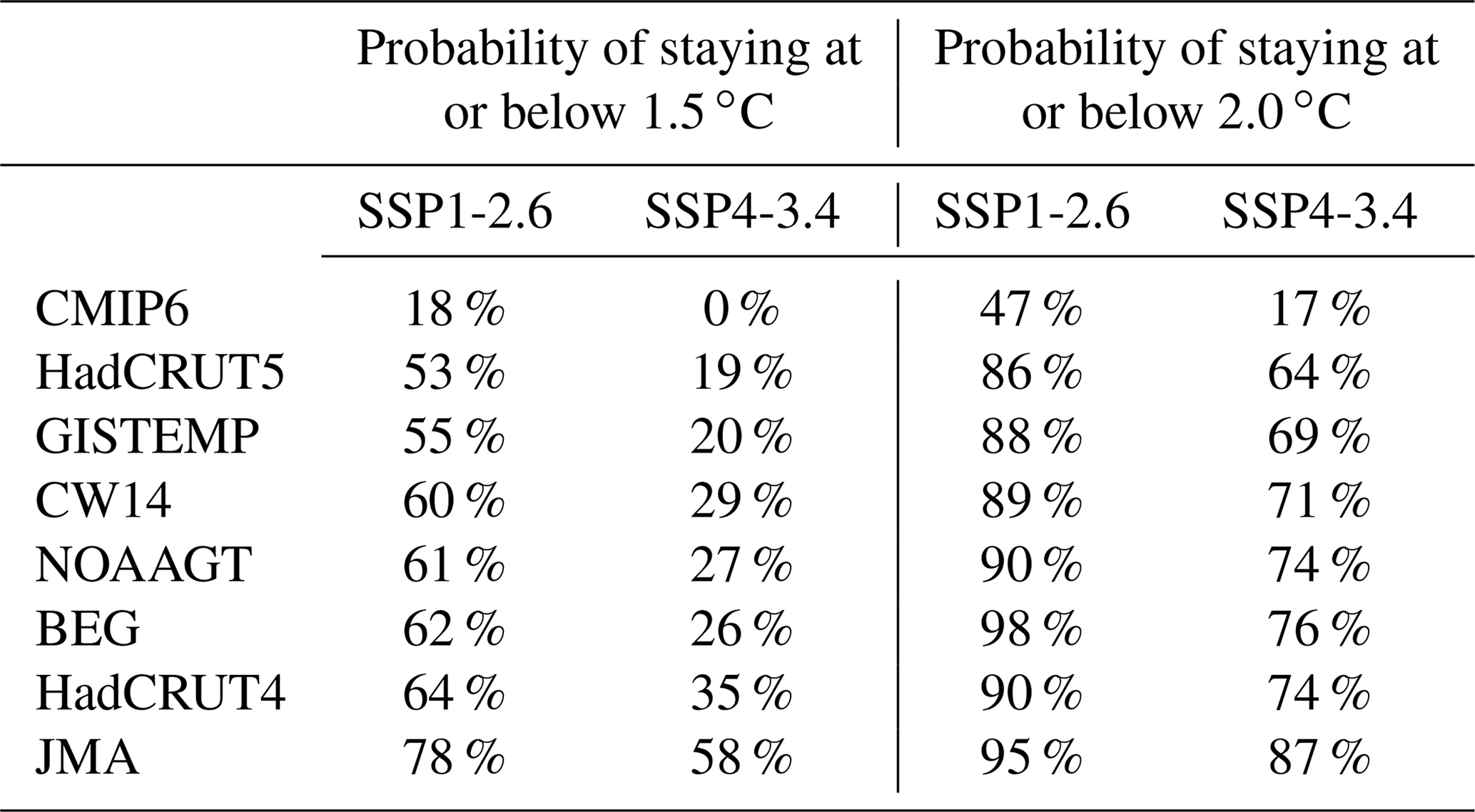
Table 2 Total cumulative and future carbon emissions that will lead to crossing the Paris temperature thresholds based on the EM-GC trained using the HadCRUT5 ΔT record. Estimates of $\mathrm{\Sigma }{\mathrm{CO}}_{\mathrm{2}}^{\mathrm{EMISSIONS}}$ that would cause global warming to stay below indicated thresholds for 95 %, 66 %, and 50 % probabilities are rounded to the nearest 10 Gt C. The values in the top half of the table are the estimates of total cumulative carbon emissions that will lead to crossing the Paris Agreement thresholds with the 10 % uncertainty for how atmospheric CO₂ responds to prescribed carbon emissions (see text) included. The values in the bottom half of the table are the estimates of future cumulative carbon emissions after 2019 that will lead to crossing the Paris Agreement thresholds with the same 10 % uncertainty. The range of years given represents when the Paris Agreement thresholds will be passed based on the rate of emissions from SSP5-8.5 or continuing the 2019 rate of emissions of 11.7 Gt C yr⁻¹ (Friedlingstein et al., 2019).

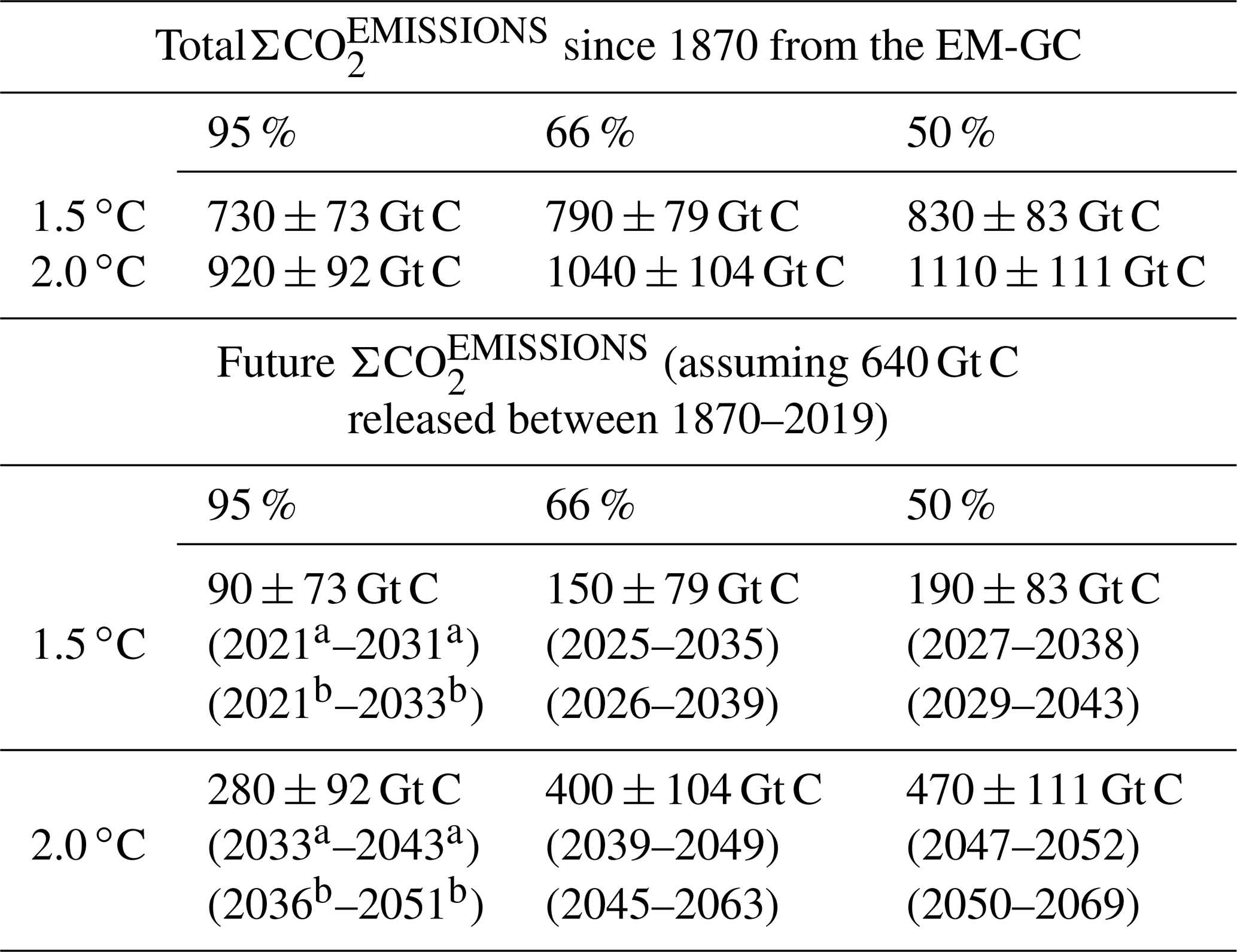
^a The year the 1.5 ^∘C target or 2.0 ^∘C upper limit will be exceeded assuming the rate of emission inferred from SSP5-8.5 and the 1σ uncertainty. Applies to the 66 % and 50 % probabilities.
^b The year the 1.5 ^∘C target or 2.0 ^∘C upper limit will be exceeded assuming the 2019 rate of emission of 11.7 Gt C yr⁻¹; the 1σ uncertainty applies to the 66 % and 50 % probabilities.

To obtain a 66 % likelihood of limiting the rise in future ΔT below 1.5 ^∘C, only 790±79 Gt C can be released. For a 66 % likelihood of the rise in ΔT staying below the 2.0 ^∘C upper limit, 1040±104 Gt C can be emitted. To place these numbers in their proper perspective, about 640 Gt C was released from 1870 through the end of 2019 due to land-use change, fossil fuel emissions, gas flaring, and cement production according to the Global Carbon Budget project (Friedlingstein et al., 2019). In our model framework, after 2019 society can therefore only emit 150±79 Gt C to have a 66 % chance of limiting warming to 1.5 ^∘C. This future emissions estimate rises to 400±104 Gt C to have a 66 % chance of limiting warming to 2.0 ^∘C.

An analysis by van Vuuren et al. (2020) assesses remaining carbon budgets based on cumulative emissions after 2010. Their analysis indicates that only 228 Gt C can be released after 2010 to have a 66 % probability of achieving the Paris Agreement target of limiting the rise in ΔT below 1.5 ^∘C in 2100. They base this estimate on an analysis of climate sensitivity and carbon cycle components, including an adjustment to TCRE for the tendency of CMIP5 GCMs to warm too quickly that was suggested by Millar et al. (2017). We find a 66 % probability of limiting warming to 1.5 ^∘C upon the release of 250±79 Gt C between 2010 and 2100. Our results are similar to the findings in van Vuuren et al. (2020). Between 2010 and 2019, about 100 Gt C was released to the atmosphere (Friedlingstein et al., 2019), so the remaining budget after 2019 for limiting warming to 1.5 ^∘C is about 128 Gt C according to van Vuuren et al. (2020). The remaining budget from our analysis is 150±79 Gt C. Our analysis and that by van Vuuren et al. (2020) suggest that at the pace of emissions in 2019 of 11.7 Gt C yr⁻¹ (Friedlingstein et al., 2019), society will cross this threshold in the next 10 years.

3.3.5 Blended methane

Atmospheric abundances of methane will likely continue to increase as society expands natural gas production and agriculture, making it important to analyze the impact of various methane scenarios on the rise in GMST. It is unlikely that future atmospheric methane abundances will progress as indicated by SSP1-2.6 (see Fig. 2), a low radiative forcing scenario. Current observations shown in Fig. 2 illustrate that the methane mixing ratio is following SSP2-4.5 and has missed the initial decline needed to follow the SSP1-2.6 pathway. To analyze the effect varying future methane abundance pathways will have on GMST, we have generated linear interpolations of the SSP1-2.6 and SSP3-7.0 methane abundances and created four alternate scenarios (see Fig. S22), which we call blended methane scenarios. We can substitute one of the blended methane scenarios into the EM-GC instead of using the projection of methane specified by the SSP database to quantify the sensitivity of future warming to various evolutions of methane in terms of the rise in GMST.

Figure 13 shows the probability of staying at or below the Paris Agreement target (gold) or upper limit (purple) for SSP1-2.6 (solid) and SSP4-3.4 (dotted) as a function of the methane mixing ratio in 2100. The lowest atmospheric methane mixing ratio value in 2100 of 1.15 ppm is from the SSP1-2.6 methane pathway, and the highest mixing ratio in 2100 of 3.20 ppm is from the SSP3-7.0 methane pathway. The four in between are the blended methane scenarios. As the atmospheric methane abundance increases, the likelihood of achieving the goals in the Paris Agreement decreases. For SSP1-2.6, the probability of limiting the rise in GMST below the 1.5 ^∘C target begins at 53 % for HadCRUT5 using the SSP1-2.6 designated methane pathway and decreases as the blended scenarios are considered. The probability of achieving the Paris Agreement target declines to 30 % if methane reaches 2.4 ppm in 2100 and to 16 % if methane increases to 3.2 ppm in 2100. Even though SSP1-2.6 can have a 53 % probability of limiting warming to 1.5 ^∘C, achieving this goal can likely only be attained through strict limits on emissions of both carbon dioxide and methane.

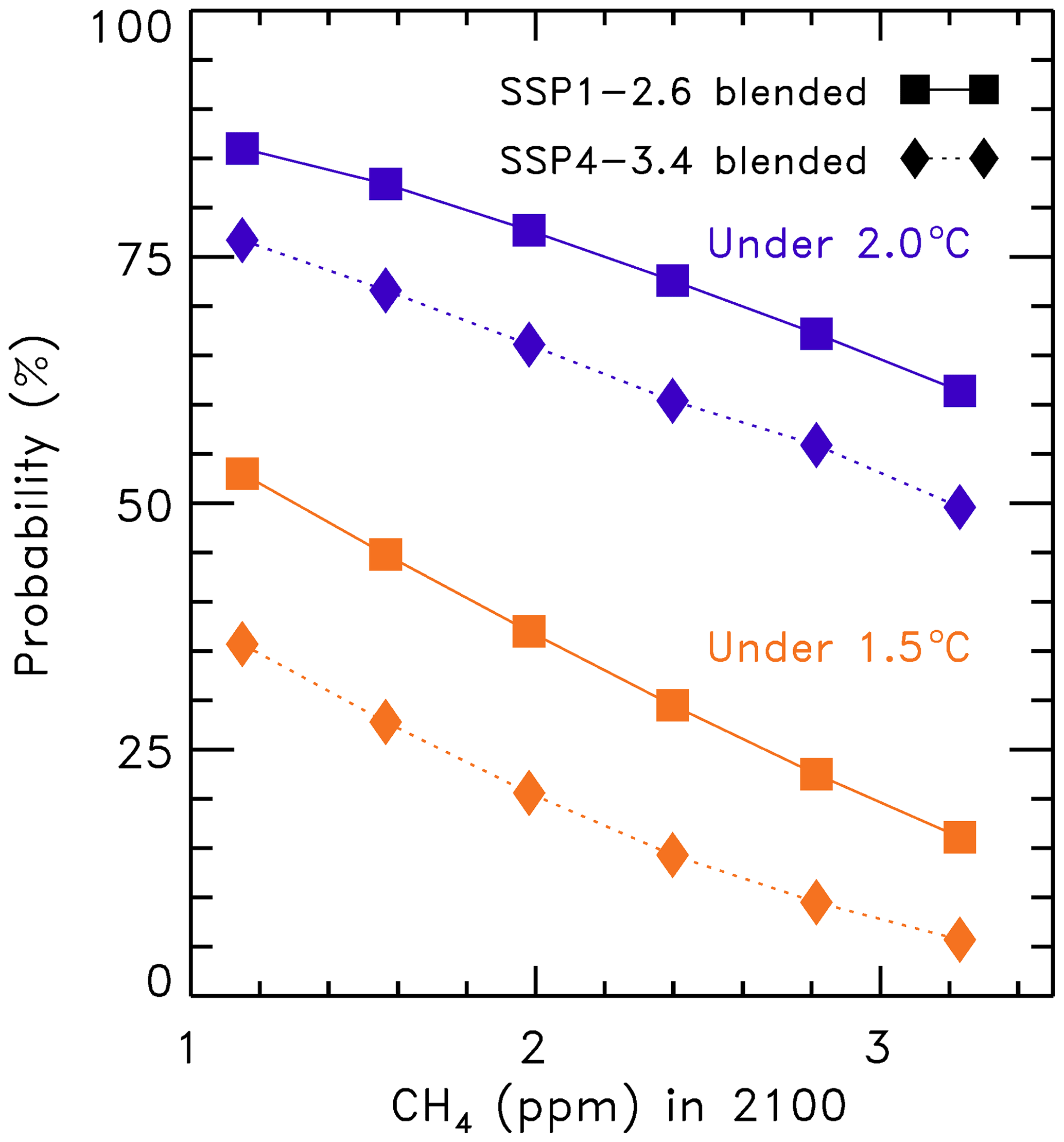
Figure 13 Probability of staying at or below the Paris Agreement target and upper limit for SSP1-2.6 and SSP4-3.4 as a function of varying methane scenarios using the EM-GC trained with the HadCRUT5 ΔT record. The atmospheric methane scenarios are calculated using linear combinations of methane abundances from SSP1-2.6 and SSP3-7.0 to span the range of future methane abundances.

In Sect. 3.3.3, we showed that if all GHGs follow the SSP4-3.4 scenario there would be a 64 % probability of limiting warming to 2.0 ^∘C. If the methane pathway instead follows SSP1-2.6, which has an end-of-century mixing ratio of only 1.15 ppm, then the probability of achieving the Paris Agreement goal rises to 77 %. If the methane pathway follows SSP3-7.0 and the end-of-century mixing ratio increases to 3.2 ppm, then the probability of achieving the Paris Agreement goal declines to 50 %.

Reducing the future anthropogenic emissions of methane might be more challenging than controlling future emissions of carbon dioxide because methane has such a wide variety of sources related to energy, agriculture, and ruminants (Kirschke et al., 2013). Given the current widespread use of methane as a source of energy in the United States and parts of Europe (Saunois et al., 2020), combined with the continued growth in the global number of ruminants (Wolf et al., 2017), it seems unrealistic for atmospheric methane to follow the peak and sharp decline starting in 2025 of the SSP1-2.6 pathway (Fig. 3b). Our analysis suggests that failure to limit methane to the SSP1-2.6 trajectory will have a larger impact on the achievement of the 1.5 ^∘C Paris goal compared to the 2.0 ^∘C upper limit. Figure 13 is designed to provide some perspective on the importance of limiting the growth of methane in the atmosphere.

3.3.6 Climate feedback

In our analysis above, we have assumed that the value of λ_Σ (and thus λ; see Eq. 3 and corresponding text in Sect. 2.1) is constant over time. Time-constant λ_Σ is the simplest assumption one can make. The climate record can be fit very well based on this conjecture, as shown in Fig. 1a. However, many GCMs suggest that climate feedback may vary over time (Dong et al., 2020; Marvel et al., 2018; Rugenstein et al., 2020). An analysis by Goodwin (2018) finds there is a delay in the response of climate feedback to a change in radiative forcing on the order of a few days to several decades. In our EM-GC framework, we are able to conduct calculations allowing the value of λ_Σ to vary over time, with a delay between the change in radiative forcing and the response of λ_Σ, and to project future temperature with such an assumption. Up until this point, our simulations have used time-invariant λ_Σ to be consistent with how our model results were presented in prior publications (Canty et al., 2013; Hope et al., 2017) and several other empirically based approaches (Chylek et al., 2014; Lean and Rind, 2008, 2009; Zhou and Tung, 2013). Recall from Sect. 2.1 that ${\mathit{\lambda }}_{\mathrm{\Sigma }}={\mathit{\lambda }}_{\mathrm{P}}-\mathit{\lambda }$. To assess the effect of time-varying climate feedback on our projections of global warming, we examine the sensitivity in terms of λ⁻¹ because this quantity scales proportionally with ΔT, and our use of the inverse λ allows for direct comparison to the results of Dong et al. (2020), Marvel et al. (2018), and Rugenstein et al. (2020).

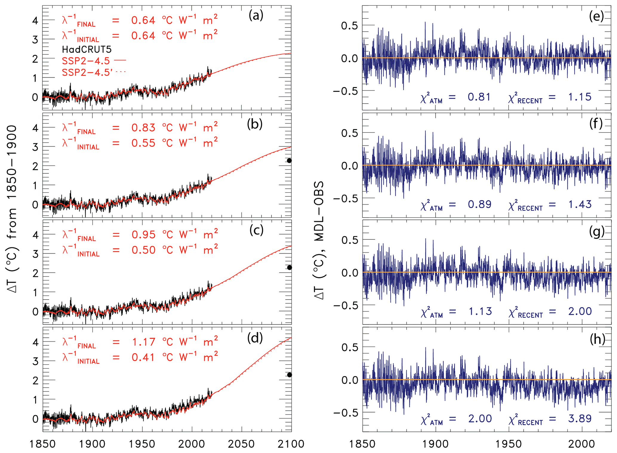
Figure 14 Change in GMST from 1850–2019 for observations from HadCRUT5 (black) and 1850–2100 modeled (red) using SSP2-4.5 and a value of AER RF${}_{\mathrm{2011}}=-\mathrm{0.9}$ W m⁻² as well as the residual between the model and observations incorporating a 32.5-year delay between λ⁻¹ and a change in RF. The solid line denotes a simulation for the original SSP2-4.5 scenario, and the dashed line indicates the SSP2-4.5' simulation (see text). (a) Rise in GMST assuming a constant value of λ⁻¹. (b) Rise in GMST allowing λ⁻¹ to increase by 50 %. (c) Rise in GMST allowing λ⁻¹ to vary, while the value of ${\mathit{\chi }}_{\mathrm{RECENT}}^{\mathrm{2}}$ is kept below 2. (d) Rise in GMST allowing λ⁻¹ to vary, while the value of ${\mathit{\chi }}_{\mathrm{ATM}}^{\mathrm{2}}$ is kept below 2. (e) Residual between the modeled and observed rise in GMST from 1850–2019 for constant λ⁻¹. (f) Same as (e) but for increasing λ⁻¹ by 50 %. (g) Same as (f) but for varying λ⁻¹, while the value of ${\mathit{\chi }}_{\mathrm{RECENT}}^{\mathrm{2}}$ is kept below 2. (h) Same as (g) but for varying λ⁻¹, while the value of ${\mathit{\chi }}_{\mathrm{ATM}}^{\mathrm{2}}$ is kept below 2.

Figure 14 shows the change in observed and modeled GMST for an EM-GC simulation training with the HadCRUT5 GMST record and using an AER RF time series with a value of AER RF${}_{\mathrm{2011}}=-\mathrm{0.9}$ W m⁻² under four assumptions for λ⁻¹, all for SSP2-4.5 (solid lines). First, the value of λ⁻¹ is constant over time (Fig. 14a, e). Second, the value of λ⁻¹ rises by 50 % between 1850–2100 (Fig. 14b, f: further discussion of Fig. 14b and f will occur at the end of this section). The third assumption allows λ⁻¹ to vary over time, while ${\mathit{\chi }}_{\mathrm{RECENT}}^{\mathrm{2}}$ is always less than or equal to 2 (Fig. 14c, g). Fourth, λ⁻¹ varies over time, while ${\mathit{\chi }}_{\mathrm{ATM}}^{\mathrm{2}}$ is always less than or equal to 2 (Fig. 14d, h). We also assume that the new time series for λ⁻¹ maintains an average value over the observational record identical to the constant value of 0.64 ^∘C W⁻¹ m². We use a lag of 32.5 years to represent the mean value of the slowest response of the climate system to an RF perturbation reported by Goodwin (2018), which is associated with clouds and spatial adjustments of SST (32.5 years is the average of 20 and 45 years, the minimum and maximum values of the slowest response given in his Table 1). Figure S23 is identical to Fig. 14, except for the use of no delay between the RF perturbations and the response of climate feedback. The use of response delays shorter than 32.5 years will result in projections between those shown in Figs. S23 and 14.

In Figs. 14 and S23 we also analyze an RF scenario termed SSP2-4.5' that serves as a doubled CO₂ scenario (dotted lines). For SSP2-4.5', the RFs due to all GHGs other than CO₂ and tropospheric aerosols from the start of 2020 onwards are held constant at end-of-2019 values. The only component of RF allowed to vary after the start of 2020 is CO₂. The RF of climate due to all GHGs and tropospheric aerosols for SSP2-4.5' is identical to that in SSP2-4.5 from the start of the simulation until the end of 2019. Since the mixing ratio of CO₂ at the end of century is 566 ppm, the warming found at the end of the century for SSP2-4.5' serves as the transient response of ΔT to rising CO₂ in our model framework. The fact that projections of ΔT found allowing only for future increases in CO₂ (dotted lines) agree so closely with those found assuming changes in RF due to all GHGs and tropospheric aerosols (solid lines) means that under the AER RF${}_{\mathrm{2011}}=-\mathrm{0.9}$ W m⁻² scaling assumption, the future change in RF due to all agents other than CO₂ nearly cancels. Projections found using the original SSP2-4.5 scenario may serve as a useful surrogate for a double CO₂ simulation. Figures S24 and S25 are the same as Fig. 14, except for the use of AER RF₂₀₁₁ values of −0.4 and −1.5 W m⁻², respectively. There are slight departures between the SSP2-4.5 and SSP2-4.5' projections of ΔT for these alternate aerosol scaling assumptions. Nonetheless, these projections are quite similar because the future decline in RF due to the assumption of declining CH₄ within SSP2-4.5 nearly balances the future increase in RF due to N₂O and all of the minor GHGs.

We fit the climate record over the past 170 years (${\mathit{\chi }}_{\mathrm{ATM}}^{\mathrm{2}}$) and past 80 years (${\mathit{\chi }}_{\mathrm{RECENT}}^{\mathrm{2}}$) extremely well for constant λ⁻¹ (Fig. 14a, e). If we allow the value of λ⁻¹ to scale with anthropogenic forcing by as much as possible such that the maximum value of ${\mathit{\chi }}_{\mathrm{RECENT}}^{\mathrm{2}}$ is always less than or equal to 2, we obtain the result shown in Fig. 14c and f. This simulation results in an increase in λ⁻¹ by nearly a factor of 2 in 2100 and a value of ΔT₂₁₀₀ of 3.4 ^∘C, about 1.0 ^∘C higher than when a constant value of λ⁻¹ is used. If we allow the value of λ⁻¹ to scale with anthropogenic forcing as much as possible such that the maximum value of ${\mathit{\chi }}_{\mathrm{ATM}}^{\mathrm{2}}$ is less than or equal to 2, we arrive at the result shown in Fig. 14d and h. This simulation yields a rise in λ⁻¹ over 2.5 centuries by a factor of 2.9 and a value of ΔT₂₁₀₀ of 4.2 ^∘C that is nearly double the estimate of ΔT₂₁₀₀ for the time-invariant λ⁻¹ (Fig. 14a). The modeled change in ΔT starts to deviate from observations around the year 1960 and persistently disagrees with the data out to present time (Fig. 14h). This simulation results in a ${\mathit{\chi }}_{\mathrm{RECENT}}^{\mathrm{2}}$ value of 3.89, which indicates poor agreement with observations.

Several other studies have investigated the amount of change in λ⁻¹. Marvel et al. (2018) suggest that the increase in the median value of ECS from the CMIP5 GCMs between the historical and abrupt 4× CO₂ simulations may be driven by an increase in λ⁻¹ of 28 % to 72 %. Rugenstein et al. (2020) estimate a median increase of 17 % for values of ECS from CMIP5 GCMs when examining millennial-length simulations compared to the 150-year Gregory et al. (2004) method, which is consistent with about an 11 % rise in λ⁻¹ (Fig. 2b of Rugenstein et al., 2020). An analysis by Dong et al. (2020) estimates a median increase in λ of +0.4 W m⁻² K⁻¹, which corresponds to a 50 % increase in λ⁻¹ (Fig. 1c, d of Dong et al., 2020). Consequently, a doubling (Fig. 14c) or almost tripling of λ⁻¹ (Fig. 14d) over 2.5 centuries is larger than the increase indicated by Marvel et al. (2018) and Dong et al. (2020) as well as the millennia-order timescale in Sect. 12.5.3 of IPCC 2013 and Rugenstein et al. (2020). An increase in λ⁻¹ of 50 % or lower (Fig. 14b) is in line with the estimate of the change in ECS due to time-variant λ⁻¹ indicated by Dong et al. (2020), Marvel et al. (2018), and Rugenstein et al. (2020).

Allowing λ⁻¹ to increase over time introduces important additional uncertainty to our estimate of ECS. We denote values of ECS found using time-variant λ⁻¹ as ECS_λ(t). Our best estimate of ECS_λ(t) is 3.08 ^∘C (range of 2.23 to 5.53 ^∘C), which is derived from model results shown in Fig. 14b (AER RF${}_{\mathrm{2011}}=-\mathrm{0.9}$ W m⁻²), Fig. S24b (AER RF${}_{\mathrm{2011}}=-\mathrm{0.4}$ W m⁻²), and Fig. S25c (AER RF${}_{\mathrm{2011}}=-\mathrm{1.5}$ W m⁻²). For this new estimate of ECS_λ(t), we allow λ⁻¹ to increase by 50 % or rise as much as possible and still achieve a value of ${\mathit{\chi }}_{\mathrm{RECENT}}^{\mathrm{2}}$ less than or equal to 2. Simulations with strong aerosol cooling (AER RF${}_{\mathrm{2011}}=-\mathrm{1.5}$ W m⁻²) cannot have λ⁻¹ rise by 50 % and maintain a good fit to the climate record over the past 80 years (Fig. S25b, f). Our best estimate of ECS_λ(t) of 3.08 ^∘C (range of 2.23 to 5.53 ^∘C) for a 32.5-year delay is similar to the value of ECS reported by Goodwin (2018) for a 100-year response time (2.9 ^∘C; range of 2.3 to 3.6 ^∘C).

The assumption of constant feedback within the EM-GC framework used in the rest of the paper is reasonable because there is no strong evidence from the climate record for a noticeable increase in λ⁻¹ on the multidecadal timescale associated with the simulations in Fig. 14. Assuming climate feedback is constant over time results in the best fits to the climate record for both of our χ² constraints. If the true value of λ⁻¹ actually rises over time as suggested by the CMIP6 (Dong et al., 2020) and CMIP5 GCMs (Marvel et al., 2018; Rugenstein et al., 2020), our projections of global warming would be a few tenths of a degree warmer than our current best estimates assuming constant λ⁻¹, as shown in Fig. 14b. If λ⁻¹ is allowed to increase by 50 %, our best estimate of ECS would rise from 2.33 to 3.08 ^∘C, which is a 32 % increase. Time-variant λ⁻¹ introduces additional uncertainty into our estimates of ECS; however, the largest uncertainty is still due to imprecise knowledge of the RF due to tropospheric aerosols.

4 Conclusions

In this paper we use a multiple linear regression energy balance model (EM-GC) to analyze and project changes in the future rise in global mean surface temperature (GMST), calculate the attributable anthropogenic warming rate (AAWR, the component of the rise in GMST caused by human activities) over the past 4 decades, and compute the effective climate sensitivity (ECS, the rise in GMST that would occur with atmospheric CO₂ at the 2× pre-industrial level assuming constant climate feedback). Projections of the rise in GMST (ΔT) are conducted for seven of the Shared Socioeconomic Pathway (SSP) projections of GHGs (O'Neill et al., 2017). We compare computations of AAWR, ECS, and projections of ΔT to values for each quantity computed from archived output provided by GCMs as part of CMIP6 (Eyring et al., 2016). A critical component of our study is a comprehensive analysis of uncertainties in AAWR, ECS, and projections of ΔT in our EM-GC framework due to the rather large uncertainty in radiative forcing of climate from tropospheric aerosols (AER RF).

The median value of AAWR from 1975–2014 computed using our EM-GC constrained by the century-and-a-half-long record for GMST provided by HadCRUT5 is 0.157 ^∘C per decade, and the 5th and 95th percentiles are 0.120 and 0.195 ^∘C per decade, respectively. The median value of AAWR from the CMIP6 multi-model ensemble is 0.221 ^∘C per decade, and the 5th and 95th percentiles are 0.151 and 0.299 ^∘C per decade, respectively. We show that the component of GMST attributed to human activity within the CMIP6 multi-model ensemble warms considerably faster than observations over the past 4 decades, a result that is consistent with recent analyses of output from the CMIP6 multi-model ensemble (CONSTRAIN, 2020; Tokarska et al., 2020b) and output from CMIP5 GCMs assessed in AR5 (i.e., Fig. 11.25b of Kirtman et al., 2013). This finding differs from the conclusion of Hausfather et al. (2020), who showed fairly good agreement between projections of global warming from GCMs and observed ΔT. As detailed in Sect. 3.1, this paper examined GCMs that preceded CMIP5 and examined ΔT for a time period that ends in 2017, a time when global temperature was influenced by a strong ENSO event that ended in 2016. The majority of the uncertainty in our EM-GC based estimate of AAWR is due to imprecise knowledge of the true value of AER RF.

In our model framework, the best estimate of ECS is 2.33 ^∘C, and the 5th and 95th percentiles are 1.40 and 3.57 ^∘C, respectively. The median value of ECS from the CMIP6 multi-model ensemble is 3.74 ^∘C, which is around 1.6 times the best-estimate value of ECS inferred from the observed climate record. The 5th and 95th percentiles of ECS from the CMIP6 multi-model ensemble are 2.19 and 5.65 ^∘C, respectively. We obtain a wide range of ECS values using the EM-GC because of the uncertainty in AER RF. With an AER RF₂₀₁₁ equal to −1.6 W m⁻², the EM-GC calculates a value of ECS similar to the maximum value of ECS from the CMIP6 multi-model mean. We cannot rule out the very high value of ECS, but we assign a low probability based on the IPCC 2013 low likelihood for the needed value of AER RF₂₀₁₁. Our empirically based determination of ECS is in good overall agreement with the recent empirical determinations of Lewis and Grünwald (2018) (1.87 ^∘C, range of 1.1-4.05 ^∘C) and Skeie et al. (2018) (2.0 ^∘C, range of 1.2–3.1 ^∘C) and the slightly older empirically determination reported by Otto et al. (2013) (2.0 ^∘C, range of 1.2–3.9 ^∘C) (all range values are for the 5th and 95th percentile confidence interval). A recent review of climate feedback and climate sensitivity published by Sherwood et al. (2020) reported that ECS lies within the range of 2.3 to 4.7 ^∘C at the 5th to 95th percentile confidence intervals; their lower bound for ECS is quite a bit higher than the lower bound found in our analysis and those by Cox et al. (2018), Dessler et al. (2018), Lewis and Grünwald (2018), Nijsse et al. (2020), Otto et al. (2013), Skeie et al. (2018), and Tokarska et al. (2020a, b). Our best estimate of ECS increases to 3.08 ^∘C (range of 2.23 to 5.53 ^∘C) if we allow climate feedback to rise over time, with the largest uncertainty in ECS still driven by imprecise knowledge of the RF due to tropospheric aerosols.

We also examined the probability of limiting the future rise in GMST below the Paris Agreement target of 1.5 ^∘C and upper limit of 2.0 ^∘C. Our probabilistic forecasts of projections of ΔT include a comprehensive treatment of the uncertainty in AER RF, a capability outside the scope of the GCM intercomparisons conducted for CMIP6. Our analysis indicates that if GHGs were to follow the SSP1-2.6 pathway, there would be a 53 % likelihood that the rise in ΔT would remain below the Paris Agreement target of 1.5 ^∘C (relative to pre-industrial) by the end of the century based on HadCRUT5. We find that the SSP4-3.4 scenario provides a 64 % likelihood of limiting global warming to below the Paris Agreement upper limit of 2.0 ^∘C by the end of the century. These probabilities declined upon our use of HadCRUT5 compared to the GMST record of HadCRUT4 to 64 % and 74 % for the SSP1-2.6 and SSP4-3.4 scenarios, respectively. In contrast, the CMIP6 multi-model mean only suggests a 18 % probability of achieving the Paris Agreement target for SSP1-2.6 and a 17 % probability of attaining the Paris Agreement goal for SSP4-3.4. The lower probabilities suggested by the CMIP6 multi-model ensemble is not surprising given the tendency of most CMIP6 GCMs to warm faster than observations over the past 4 decades. Our projections of ΔT using a physically based model tied to observations of ocean heat content, quantification of natural and anthropogenic drivers of variations in GMST, and consideration of uncertainty in AER RF are shown to be remarkably similar to the expert assessment of the future rise in GMST that was sketched out in Fig. 11.25b of AR5 (Kirtman et al., 2013) and the empirically based filtering of CMIP6 model output recently published by Tokarska et al. (2020b). Finally and most importantly, our estimates are based on the assumption that climate feedback has been and will continue to remain constant over time, since the prior temperature record can be fit so well under this assumption. As described in Sect. 3.3.6, if climate feedback rises over time, larger warming will be realized than that found under this assumption of temporally invariant feedback.

We also quantify the sensitivity of the probability of achieving the Paris Agreement target (1.5 ^∘C) or upper limit (2.0 ^∘C) to future atmospheric abundances of methane. The end-of-century mixing ratio of methane in the SSP1-2.6 scenario is 1.15 ppm, considerably less than the contemporary abundance of 1.88 ppm. The likelihood of attaining the 1.5 ^∘C target for SSP1-2.6 decreases as future methane emissions increase; it declines to 30 % if methane reaches 2.4 ppm in 2100 and to 16 % if methane increases to 3.2 ppm at the end of the century. Our analysis described in Sect. 3.3.5 demonstrates that major near-term limits on the future growth of methane are especially important for achievement of the 1.5 ^∘C limit to future warming that constitutes the goal of the Paris Agreement.

Finally, we have also quantified in the EM-GC framework the remaining budgets of carbon (i.e., CO₂) emissions that can occur while attaining either the goal or upper limit of the Paris Agreement. We find that after 2019, society can only emit another 150±79 Gt C to have a 66 % likelihood of limiting warming to 1.5 ^∘C. This future emissions estimate rises to 400±104 Gt C to have a 66 % probability of limiting warming to 2.0 ^∘C. Given that the anthropogenic emissions of carbon due to combustion of fossil fuels, cement production, gas flaring, and land-use change were about 11.7 Gt C per year in 2019 (Friedlingstein et al., 2019), our study indicates that the target (1.5 ^∘C warming) of the Paris Agreement will not be achieved unless carbon emissions are severely curtailed in the next 10 years.

We conclude by noting that the CMIP6 multi-model ensemble provides many useful parameters, such as sea level rise, sea ice decline, and precipitation changes, that provide a great societal understanding of the impact of climate change. We do not mean to undermine the importance of the CMIP6 GCMs with this analysis. Rather, we hope that studies such as this, along with other recent evaluations of CMIP6 multi-model output like Nijsse et al. (2020) and Tokarska et al. (2020b), will lead to improved use of the CMIP6 multi-model ensemble for policy decisions. Our EM-GC was built to specifically simulate and project changes in GMST; we do not examine numerous other components of the climate system that affect society. We emphasize that our projections show that unless society can implement steep reductions in the emissions of carbon and methane in the next 10 years, the 1.5 ^∘C global warming goal of the Paris Agreement will not be achieved.

Appendix A: Acronyms

AAWR	Attributable anthropogenic warming rate
AR4	Fourth Assessment Report
AER	Anthropogenic aerosol
AER RF2011	Radiative forcing due to anthropogenic aerosols in 2011
AMOC	Atlantic Meridional Overturning Circulation
AMV	Atlantic multidecadal variability
BEG	Berkeley Earth Group
CALIPSO	Cloud–Aerosol Lidar and Infrared Pathfinder Satellite Observations
CMIP5	Coupled Model Intercomparison Project Phase 5
CMIP6	Coupled Model Intercomparison Project Phase 6
COBE	Centennial in situ Observation-Based Estimate
CW14	Cowtan and Way (2014) temperature record
ECS	Effective climate sensitivity
ECSλ(t)	Effective climate sensitivity, time-dependent feedback
EM-GC	Empirical Model of Global Climate
ENSO	El Niño–Southern Oscillation
GCM	General circulation model
GHG	Greenhouse gas
GISTEMP	Goddard Institute for Space Studies Surface Temperature Analysis
v4 GloSSAC	Global Space-based Stratospheric Aerosol Climatology
GMST	Global mean surface temperature
HadCRUT	Hadley Centre Climatic Research Unit
IPCC	Intergovernmental Panel on Climate Change
ISCCP	International Satellite Cloud Climatology Project
IOD	Indian Ocean Dipole
LIN	Linear method
LUC	Land-use change
MEI	Multivariate ENSO index
NOAAGT	National Center for Environmental Information NOAAGlobalTemp v5
ODS	Ozone-depleting substance
OHC	Ocean heat content
OHE	Ocean heat export
PATMOS-X	Pathfinder Atmospheres Extended
PDO	Pacific Decadal Oscillation
RCP	Representative Concentration Pathway
REG	Regression method
RF	Radiative forcing
SAOD	Stratospheric aerosol optical depth
SORCE	Solar Radiation and Climate Experiment
SSP	Shared Socioeconomic Pathway
SST	Sea surface temperature
TAR	Third Assessment Report
TAS	Near-surface air temperature
TCRE	Transient climate response to cumulative emissions
TOS	Temperature at the interface of the atmosphere and the upper boundary of the ocean
TSI	Total solar irradiance