the Creative Commons Attribution 4.0 License.
the Creative Commons Attribution 4.0 License.
 | 13 Nov 2020
Reduced global warming from CMIP6 projections when weighting models by performance and independence
Angeline G. Pendergrass
Flavio Lehner
Anna L. Merrifield
Ruth Lorenz
Reto Knutti
The sixth Coupled Model Intercomparison Project (CMIP6) constitutes the latest update on expected future climate change based on a new generation of climate models. To extract reliable estimates of future warming and related uncertainties from these models, the spread in their projections is often translated into probabilistic estimates such as the mean and likely range. Here, we use a model weighting approach, which accounts for the models' historical performance based on several diagnostics as well as model interdependence within the CMIP6 ensemble, to calculate constrained distributions of global mean temperature change. We investigate the skill of our approach in a perfect model test, where we use previous-generation CMIP5 models as pseudo-observations in the historical period. The performance of the distribution weighted in the abovementioned manner with respect to matching the pseudo-observations in the future is then evaluated, and we find a mean increase in skill of about 17 % compared with the unweighted distribution. In addition, we show that our independence metric correctly clusters models known to be similar based on a CMIP6 “family tree”, which enables the application of a weighting based on the degree of inter-model dependence. We then apply the weighting approach, based on two observational estimates (the fifth generation of the European Centre for Medium-Range Weather Forecasts Retrospective Analysis – ERA5, and the Modern-Era Retrospective analysis for Research and Applications, version 2 – MERRA-2), to constrain CMIP6 projections under weak (SSP1-2.6) and strong (SSP5-8.5) climate change scenarios (SSP refers to the Shared Socioeconomic Pathways). Our results show a reduction in the projected mean warming for both scenarios because some CMIP6 models with high future warming receive systematically lower performance weights. The mean of end-of-century warming (2081–2100 relative to 1995–2014) for SSP5-8.5 with weighting is 3.7 ∘C, compared with 4.1 ∘C without weighting; the likely (66%) uncertainty range is 3.1 to 4.6 ∘C, which equates to a 13 % decrease in spread. For SSP1-2.6, the weighted end-of-century warming is 1 ∘C (0.7 to 1.4 ∘C), which results in a reduction of −0.1 ∘C in the mean and −24 % in the likely range compared with the unweighted case.
- Article
(2897 KB) - Full-text XML
-
Supplement
(1783 KB) - BibTeX
- EndNote


Projections of future climate by Earth system models provide a crucial source of information for adaptation planing, mitigation decisions, and the scientific community alike. Many of these climate model projections are coordinated and provided within the frame of the Coupled Model Intercomparison Projects (CMIPs), which are now in phase 6 (Eyring et al., 2016). A typical way of communicating information from such multi-model ensembles (MMEs) is through a best estimate and an uncertainty range or a probabilistic distribution. In doing so, it is important to make sure that the different sources of uncertainty are identified, discussed, and accounted for, in order to provide reliable information without being overconfident. In climate science, three main sources of uncertainty are typically identified in MMEs: (i) uncertainty in future emissions, (ii) internal variability of the climate system, and (iii) model response uncertainty (e.g., Hawkins and Sutton, 2009; Knutti et al., 2010).
Uncertainty due to future emissions can easily be isolated by making projections conditional on scenarios such as the Shared Socioeconomic Pathways (SSPs) in CMIP6 (O'Neill et al., 2014) or the Representative Concentration Pathways (RCPs) in CMIP5 (van Vuuren et al., 2011). The other two sources of uncertainty are harder to quantify, as reliably separating them is often challenging (e.g., Kay et al., 2015; Maher et al., 2019). Model uncertainty (sometimes also referred to as structural uncertainty or response uncertainty) is used here to describe the differing responses of climate models to a given forcing due to their structural differences following the definition by Hawkins and Sutton (2009). Such different responses to the same forcing can emerge due to different processes and feedbacks as well as due to the parametrization used in the different models, among other things (e.g., Zelinka et al., 2020).
In this paper, internal variability refers to a model's sensitivity to the initial conditions as captured by initial-condition ensemble members (e.g., Deser et al., 2012). In this sense, it stems from the chaotic behavior of the climate system at different timescales and is highly dependent on the variable of interest as well as the period and region considered. While, for example, uncertainty in global mean temperature is mainly dominated by differences between models, the regional temperature trends are considerably more dependent on internal variability. Recently, efforts have been made to use so-called single model initial-condition large ensembles (SMILEs) to investigate internal variability in the climate projections more comprehensively (e.g., Kay et al., 2015; Maher et al., 2019; Lehner et al., 2020; Merrifield et al., 2020).
Depending on the composition of the MME investigated, uncertainty estimates often fail to reflect the fact that included models are not independent of one another. In the development process of climate models, ideas, code, and even full components are shared between institutions, or models might be branched from one another in order to investigate specific questions. This can lead to some models (or model components) being copied more often, resulting in an overrepresentation of their respective internal variability or sensitivity to forcing (Masson and Knutti, 2011; Bishop and Abramowitz, 2013; Knutti et al., 2013; Boé and Terray, 2015; Boé, 2018). The CMIP MMEs in particular have not been designed with the aim of including only independent models and are, therefore, sometimes referred to as “ensembles of opportunity” (e.g., Tebaldi and Knutti, 2007), incorporating as many models as possible. Thus, when calculating probabilities based on such MMEs it is important to account for model interdependence in order to accurately translate model spread into estimates of mean change and related uncertainties (Knutti, 2010; Knutti et al., 2010).
In addition, not all models represent the aspects of the climate system relevant to a given question equally well. To account for this, a variety of different approaches have been used to weight, sub-select, or constrain models based on their historical performance. This has been done both regionally and globally as well as for a range of different target metrics such as end-of-century temperature change or transient climate response (TCR); for an overview, the reader is referred to studies such as Knutti et al. (2017a), Eyring et al. (2019), and Brunner et al. (2020b). Global mean temperature increase in particular is one of the most widely discussed effects of continuing climate change and the main focus of many public and political discussions. With the release of the new generation of CMIP6 models, this discussion has been sparked yet again, as several CMIP6 models show stronger warming than most of the earlier-generation CMIP5 models (Andrews et al., 2019; Gettelman et al., 2019; Golaz et al., 2019; Voldoire et al., 2019; Swart et al., 2019; Zelinka et al., 2020; Forster et al., 2020). This raises the question of whether these models are accurate representations of the climate system and what that means for the interpretation of the historical climate record and the expected change due to future anthropogenic emissions.
Here, we use the climate model weighting by independence and performance (ClimWIP) method (e.g., Knutti et al., 2017b; Lorenz et al., 2018; Brunner et al., 2019; Merrifield et al., 2020) to weight models in the CMIP6 MME. Weights are based on (i) each model's performance with respect to simulating historical properties of the climate system, such as horizontally resolved anomaly, variability, and trend fields, and (ii) its independence from the other models in the ensemble, which is estimated based on the shared biases of climatology. In contrast to many other methods that constrain model projections based on only one observable quantity, such as the warming trend (e.g., Giorgi and Mearns, 2002; Ribes et al., 2017; Jiménez-de-la Cuesta and Mauritsen, 2019; Liang et al., 2020; Nijsse et al., 2020; Tokarska et al., 2020), ClimWIP is based on multiple diagnostics, representing different aspects of the climate system. These diagnostics are chosen to evaluate a model's performance with respect to simulating observed climatology, variability, and trend patterns. Note that, in contrast to other approaches such as emergent constraint-based methods, some of these diagnostics might not be highly correlated with the target metric (however, it is still important that they are physically relevant in order to avoid introducing noise without useful information in the weighting). Combining a range of relevant diagnostics is less prone to overconfidence, as the risk of up-weighting a model because it “accidentally” fits observations for one diagnostic while being far away from them in several others is greatly reduced. In turn, methods that are based on such a basket of diagnostics have been found to generally lead to weaker constraints (Sanderson et al., 2017; Brunner et al., 2020b), as the effect of the weighting typically weakens when adding more diagnostics (Lorenz et al., 2018).
ClimWIP has already been used to create estimates of regional change and related uncertainties for a range of different variables such as Arctic sea ice (Knutti et al., 2017b), Antarctic ozone concentrations (Amos et al., 2020), North American maximum temperature (Lorenz et al., 2018), and European temperature and precipitation (Brunner et al., 2019; Merrifield et al., 2020). Recently, Liang et al. (2020) used an adaptation of the method to constrain changes in global temperature using the global mean temperature trend as the single diagnostic for both the performance and independence weighting. Here, we focus on investigating the ClimWIP method's performance in weighting global mean temperature changes when informed by a range of diagnostics. To assess the robustness of these choices, we perform an out-of-sample perfect model test using CMIP5 and CMIP6 as pseudo-observations. Based on these results, we select a combination of diagnostics that capture not only a model's transient warming but also its ability to reproduce historical patterns in climatology and variability fields; this is done in order to increase the robustness of the weighting scheme and minimize the risk of skill decreases due to the weighting. This approach is particularly important for users interested in the “worst case” rather than in mean changes. We also look into the interdependencies among the models, showing the ability of our diagnostics in clustering models with known shared components using a “family tree” (Masson and Knutti, 2011; Knutti et al., 2013), and we further show the skill of the independence weighting to account for this. We then calculate combined performance–independence weights based on two reanalysis products in order to also account for the uncertainty in the observational record. Finally, we apply these weights to provide constrained distributions of future warming and TCR.
2.1 Model data
The analysis is based on all currently available CMIP6 models that provide surface air temperature (tas) and sea level pressure (psl) for the historical, SSP1-2.6, and SSP5-8.5 experiments. We use all available ensemble members, which results in a total of 129 runs from 33 models (see Table S4 for a full list including references). We use models post-processed within the ETH Zurich CMIP6 next generation archive, which provides additional quality checks and re-grids models onto a common latitude–longitude grid, using second-order conservative remapping (see Brunner et al., 2020a, for details). In addition, we use one member of all CMIP5 models providing the same variables and the corresponding experiments (historical, RCP2.6, and RCP8.5), which results in a total of 27 models (see Table S5 for a full list).
2.2 Reanalysis data
To represent historical observations in tas and psl, we use two reanalysis products: ERA5 (C3S, 2017) and MERRA-2 (GMAO, 2015a, b; Gelaro et al., 2017). Both products are re-gridded to a latitude–longitude grid using second-order conservative remapping and are evaluated in the period from 1980 to 2014. We use a combination of these two observational datasets following the results of Lorenz et al. (2018) and Brunner et al. (2019), who show that using individual datasets separately can lead to diverging results in some cases. It has been argued that combining multiple datasets (e.g., by using their full range or their mean) yields more stable results (Gleckler et al., 2008; Brunner et al., 2019). Here, we use the mean of ERA5 and MERRA-2 at each grid point as reference equivalent to Brunner et al. (2019). Finally, we also compare our results to globally averaged merged temperatures from the Berkeley Earth Surface Temperature (BEST) dataset (Cowtan, 2019).
2.3 Model weighting scheme
We use an updated version of the ClimWIP method described in Brunner et al. (2019) and Merrifield et al. (2020), which is based on earlier work by Lorenz et al. (2018), Knutti et al. (2017b), and Sanderson et al. (2015b, a); it can be downloaded at https://github.com/lukasbrunner/ClimWIP.git (last access: 8 October 2020). It assigns a weight wi to each model mi that accounts for both model performance and independence:
where Di and Sij are the generalized distances of model mi to the observations and to model mj, respectively. The shape parameters σD and σS set the strength of the weighting, effectively determining the point at which a model is considered to be “close” to the observations or to another model (see Sect. 2.5).
This updated version of ClimWIP assigns the same weight to each initial-condition ensemble member of a model, which is adjusted by the number of ensemble members (see Merrifield et al., 2020, for a detailed discussion). To illustrate this additional step in the weighting method, consider a single performance diagnostic d. d is calculated for each model and ensemble member separately; hence, , where i represents individual models and k runs over all ensemble members Ki of model mi (from 1 to 50 members in CMIP6). For each model mi, the mean diagnostic is
is then used to calculate the generalized distance Di and further the performance weight wi via Eq. (1). A detailed description of this processing chain can be found in Sect. S2. An analogous process is used for distances between models. This setup allows for a consistent comparison of model fields to one another and to observations in the presence of internal variability and, in particular, also enables the use of variance-based diagnostics. In addition, it ensures a consistent estimate of the performance shape parameter σD in the calibration (see Sect. 2.5), based on the average weight per model; in previous work, in contrast, the calibration was based on only one ensemble member per model.
2.4 Weighting target and diagnostics
We apply the weighting to projections of the annual-mean global-mean temperature change from two SSPs, representing weak (SSP1-2.6) and strong (SSP5-8.5) climate change scenarios. Changes in two 20-year target periods representing mid-century (2041–2060) and end-of-century (2081–2100) conditions are compared to a 1995–2014 baseline. In addition, we weight TCR values obtained from an update of the dataset described in Tokarska et al. (2020). The weights are calculated from global, horizontally resolved diagnostics based on annual mean data in the 35-year period from 1980 to 2014. We use different diagnostics for the calculation of the independence and performance parts of the weighting, as proposed in Merrifield et al. (2020).
The goal of the independence weighting is to identify structural similarities between models (such as shared offsets or similar spatial patterns) which are interpreted to be indications of interdependence arising from factors such as shared components or parameterizations. In the past, combinations of horizontally resolved regional temperature, precipitation, and sea level pressure fields have typically been used (e.g., Knutti et al., 2013; Sanderson et al., 2017; Boé, 2018; Lorenz et al., 2018; Brunner et al., 2019). Building on the work of Merrifield et al. (2020), we use a combination of two global, climatology-based diagnostics, the spatial pattern of climatological temperature (tasCLIM) and sea level pressure (pslCLIM), as similar diagnostics were found to work well for clustering CMIP5-generation models known to be similar. Beside our approach, several other methods to tackle this issue of model dependence exist. Among them are approaches that use other metrics to establish model independence (e.g., Pennell and Reichler, 2011; Bishop and Abramowitz, 2013; Boé, 2018), approaches that select a more independent subset of the original ensemble (e.g., Leduc et al., 2016; Herger et al., 2018a), or even approaches that treat model similarity as an indication of robustness and give models that are closer to the multi-model mean more weight (e.g., Giorgi and Mearns, 2002; Tegegne et al., 2019). Neither of these definitions of independence hold in a strictly statistical sense (Annan and Hargreaves, 2017), but we still stress that it is important to account for different degrees of model interdependence as well as possible when developing probabilistic estimates from an “ensemble of opportunity” such as CMIP6. Additional discussion about our method for calculating model independence in the context of other approaches can be found in Sect. S4.
The performance weighting, in turn, allocates more weight to models that better represent the observed behavior of the climate system as measured by the diagnostics while down-weighting models with large discrepancies from the observations. We use multiple diagnostics to limit overconfidence in cases where a model fits the observations well in one diagnostic by chance while being far away from them in several others. For example, we want to avoid giving heavy weight to a model based solely on its representation of the temperature trend if its year-to-year variability differs strongly from the observed year-to-year variability. The performance weights are based on five global, horizontally resolved diagnostics: temperature anomaly (tasANOM; calculated from tasCLIM by removing the global mean), temperature variability (tasSTD), sea level pressure anomaly (pslANOM), sea level pressure variability (pslSTD), and the temperature trend (tasTREND). A detailed description of the diagnostic calculation can be found in Sect. S2. We use anomalies instead of climatologies in the performance weight in order to avoid punishing models for absolute bias in global-mean temperature and pressure, because these are not correlated with projected warming (Flato et al., 2013; Giorgi and Coppola, 2010). This can be different for regional cases, where, for example, absolute temperature biases have been shown to be important for constraining projections of the Arctic sea ice extent (Knutti et al., 2017b) or European summer temperatures (Selten et al., 2020).
One aim of our study is to find an optimal combination of diagnostics that successfully constrains projections for our target quantity (global temperature change) while avoiding overconfidence or susceptibility to uncertainty from internal variability. For example, tasTREND is a powerful diagnostic due to its clear physical relationship and high correlation with projected warming (e.g., Nijsse et al., 2020; Tokarska et al., 2020). However, while it has the highest correlation with the target of all investigated diagnostics, it also has the largest uncertainty due to internal variability (i.e., the spread of tasTREND across ensemble members of the same model). Ideally, a performance weight is reflective of underlying model properties and does not depend on which ensemble member is chosen to represent that model. tasTREND does not fulfill this requirement: the spread within one model is the same order of magnitude as the spread among different models. To find a compromise, we divide our diagnostics into two groups: trend-based diagnostics (tasTREND) and non-trend-based diagnostics (tasANOM, tasSTD, pslANOM, and pslSTD). Different combinations of these two groups (ranging from only non-trend-based diagnostics to only tasTREND) are evaluated in Sect. 3.1, and the best performing combination is selected for the remainder of the study.
2.5 Estimation of the shape parameters
The shape parameters σD and σS are two constants that determine the width of the Gaussian weighting functions for all models. As such, they are responsible for translating the generalized distances into weights. Regarding the performance weighting, small values of σD lead to aggressive weighting, with a few models receiving all the weight, whereas large values lead to more equal weighting. It is important to note that, while σD sets this “strength” of the weighting, the rank of a model (i.e., where it lies on the scale from best to worst) is purely based on its generalized distance to the observations. To estimate a performance shape parameter σD that weights models based on their historical performance without being overconfident, we use a calibration approach based on the perfect model test in Knutti et al. (2017b) and detailed in Sect. S3. In short, the calibration selects the smallest σD value (hence, the strongest weighting) for which 80 % of “perfect models” fall within the 10–90 percentile range of the weighted distribution in the target period. Smaller σD values lead to less models fulfilling this criterion and, hence, to overly narrow, overconfident projections. Note that methods that simply maximize the correlation of the weighted mean to the target often tend to pick small values of σD that result in projections that are overconfident in the sense that the uncertainty ranges are too small (Knutti et al., 2017b). A similar issue arises for methods that estimate σD based only on historical information, as better performance in the base state does not necessarily lead to a more skilled representation of the future – for example, if the chosen diagnostics are not relevant for the target (Sanderson and Wehner, 2017).
The independence weighting has a subtle but fundamentally different dependence on its shape parameter σS: small values lead to equal weighting, as all models are considered to be independent, but so do large values, as all models are considered to be dependent. Hence, the effect of the independence weighting is strongest if the shape parameter is chosen such that it identifies clusters of models as similar (down-weighting them) while still correctly identifying models that are far from each other as independent (hence, giving them relatively more weight). For a detailed discussion including SMILEs, see Merrifield et al. (2020). To estimate σS, we use the information from models with more than one ensemble member. Simply put, we know that initial-condition ensemble members are copies of the same model that differ only due to internal variability; therefore, we have some information about the distances that must be considered “close” by σS. The method for calculating σS is described in detail in Sect. 3 of the Supplement of Brunner et al. (2019). Here, we arrive at a value of σS=0.54, which we use throughout the paper. It is worth noting that σS is based only on historical model information; therefore, it is independent of observations or the selected target period and scenario. Additional discussion of the selected σS value in the context of the multi-model ensemble used in this study can be found in the Sect. S5.
2.6 Validation of the performance weighting
To investigate the skill of ClimWIP in weighting CMIP6 global mean temperature change and the effect of the different diagnostic combinations, we apply a perfect model test (Abramowitz and Bishop, 2015; Boé and Terray, 2015; Sanderson et al., 2017; Knutti et al., 2017b; Herger et al., 2018a, b; Abramowitz et al., 2019). As a skill measure, we use the continuous ranked probability skill score (CRPSS), a measure of the ensemble forecast quality, defined as the relative error between the distribution of weighted models and a reference (Hersbach, 2000). Here, we use the relative CRPSS change between the unweighted and weighted cases (in percent), with positive values indicating a skill increase. The CRPSS is calculated separately for both SSPs and future time periods, as we expect to find different skill for different projected climate states.
The first perfect model test only focuses on the relative skill differences when applying performance weights based on different combinations of diagnostics (results are presented in Sect. 3.1). We explain its implementation based on an example perfect model mj with only one ensemble member for simplicity here: (i) the model mj is taken as a pseudo-observation and removed from the CMIP6 MME; (ii) the output from mj during the historical diagnostic period (1980–2014) is used to calculate the performance diagnostics for the remaining models (); (iii) the generalized model–“observation” distances (Di≠j) and the performance weights (wi≠j) are calculated and applied to the MME (excluding mj); (iv) the CRPSS is calculated in the target periods using the future projections of mj as reference. This is done iteratively, using each model in CMIP6 MME in turn as a pseudo-observation. For perfect models with more than one ensemble member (), all members are removed from the ensemble in (i), is calculated for each member separately in (ii) and then averaged, and the CRPSS is also calculated for each ensemble member in (iv) and averaged.
This approach is structurally similar to the one used to calibrate the performance shape parameter σD as an integral part of ClimWIP (described in Sect. 2.5). However, the metric and aim of this perfect model test are quite different. It is used to show the potential for a skill increase through the performance weighting as well as the risk of a decrease based on the selected σD and to establish the most skillful combination of diagnostics.
The second perfect model test (Sect. 3.2) is conceptually similar, but pseudo-observations are now drawn from CMIP5 instead of CMIP6. This test has the advantage that the perfect models have not been used to estimate σD and can be considered independent. However, one might also argue that the CMIP5 pseudo-observations are not fully out-of-sample, as several CMIP6 models are related to CMIP5 models and might be structurally similar to their predecessors, which was the case for the CMIP5 and CMIP3 generations (Knutti et al., 2013). However, there are also considerable differences between CMIP5 and CMIP6 that arise from many years of additional model development, a longer observational record to calibrate to, and differing spatial resolutions. In addition, the emission scenarios that force CMIP5 and CMIP6 in the future (RCPs and SSPs, respectively) result in slightly different radiative forcings (Forster et al., 2020), and several CMIP6 models have been shown to lead to considerably more warming than most CMIP5 models. We do not discuss these similarities and differences between the model generations in detail here; instead, we simply use CMIP5 as a source of pseudo-observations to evaluate the skill of ClimWIP in weighting the CMIP6 MME. To avoid cases with the highest potential for remaining dependence between generations, we exclude CMIP6 models that are direct predecessors of the respective CMIP5 model used as pseudo-observations (see Table S5 for a list).
2.7 Validation of the independence weighting
To validate that the information in the diagnostics chosen for the independence weighting (tasCLIM and pslCLIM) can identify models known to be similar, we use a hierarchical clustering approach based on Müllner (2011) and implemented in the Python SciPy package (https://www.scipy.org/, v1.5.2). We use the linkage function with the average method applied to the horizontally resolved distance fields between each pair of models (see Sect. S6 for more details). This approach is conceptually similar to the work of Masson and Knutti (2011) and Knutti et al. (2013) and follows their example of showing similarity as model “family trees”. The hierarchical clustering is not used in the model weighting itself; we use it here only to show that qualitative information about model similarity can be inferred from model output using the two chosen diagnostics and to compare it to the results from the independence weighting.
The independence weighting (denominator in Eq. 1) quantifies the similarity information extracted from the pairwise distance fields via the independence shape parameter (σS; see Sect. 2.5). The independence weighting estimates where two models fall on the spectrum from completely independent to completely redundant and weights them accordingly. In order to test this approach, we successively add artificial “new” models into the CMIP6 MME: for an example model with two members ( and ), we remove the first member and add it as an additional model (mM+1). In an idealized case, where all models are perfectly independent of one another and all ensemble members of a model are identical, we would expect the weight of the member that remains () to go down by a factor of 1∕2, while the weight of all other models would stay the same. However, in a real MME, where there is internal variability and complex model interdependencies exist, we would not necessarily expect such simple behavior; several other models might also be (rightfully) affected by adding such a duplicate, and the effect on the would be smaller (see Sect. 4.2)
3.1 Leave-one-out perfect model test with CMIP6
We start by calculating the performance weights in the diagnostic period (1980–2014) in a pure model world and without using the independence weighting. In this first step, we focus on relative skill differences when using different combinations of diagnostics. Figure 1 shows the distribution of the CRPSS (with positive values indicating an increase in projection skill due to the weighting and vice versa; see Sect. 2.6) evaluated for the mid- and end-of-century target periods, the two SSPs, and for different combinations of diagnostics. The diagnostics range from only non-trend-based diagnostics (0 % tasTREND + 25 % tasANOM + 25 % tasSTD + 25% pslANOM + 25 % pslSTD = 100 %) to only trend-based diagnostics (100 % tasTREND). Overall, all diagnostic combinations tend to increase median skill compared with the unweighted projections, but there is a considerable range of CRPSS values and they can be negative. In evaluating the different cases, we consequently focus on two important aspects of the CRPSS distribution: (i) the median, as a best estimate of the expected relative skill change, and (ii) the 5th and 25th percentiles, in particular if they are negative. Negative CRPSS values indicate a worsening of the projections compared with the unweighted case. As the goal of the weighting is to improve the projections based on the performance and dependence of the models, the risk of negative CRPSSs should be minimized.
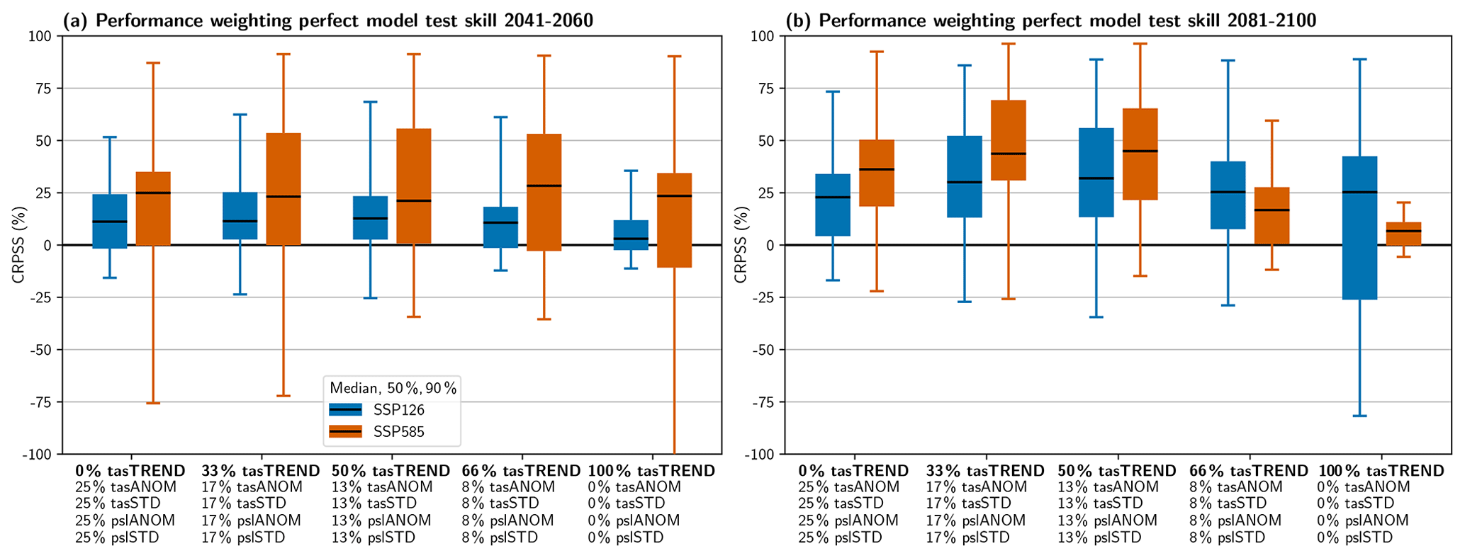
Figure 1Continuous ranked probability skill score (CRPSS) relative to the unweighted ensemble for the performance weighting based on a leave-one-out perfect model test with CMIP6 for (a) mid-century and (b) end-of-century temperature change relative to 1995–2014. The x axis shows different combinations of the two diagnostic groups ranging from only non-trend-based diagnostics (0 % tasTREND) to only trend-based diagnostics (100 % tasTREND). The values not summing to 100 % is due to rounding in the labels only.
We find the σD values to be correctly calibrated by the method in order to limit the risk of a strong skill decrease (the CRPSS is close to zero or positive for the 25th percentile in almost all cases). For the mid-century period, the median skill increases by up to 25 % depending on the SSP and the combination of diagnostics. The magnitude of potential negative CRPSSs in a “worst-case” scenario (5th percentile), however, is better constrained using a balanced combination of diagnostics (e.g., 50 % tasTREND). In the end-of-century period, the median skill is more variable (mainly due to the selected performance shape parameters σD; see Table S1 in the Supplement), with combinations that include both trend and non-trend diagnostics again performing best.
Using 50 % tasTREND and 50 % anomaly- and variance-based diagnostics (about 13 % tasANOM, 13 % tasSTD, 13 % pslANOM, and 13 % pslSTD) optimizes the combination of median CRPSS increases and the avoidance of possible negative CRPSSs; therefore, we use this combination to calculate the weights for the rest of the analysis. Note that the two SSPs and time periods have slightly different σD values (ranging from 0.35 to 0.58; Table S1), leading to slightly differing weights even though the historical information is the same. This arises from differences in confidence when applying the method for different targets. However, as the σD values are found to be so similar, we use the mean value from the two SSPs and time periods in the following for simplicity; hence, σD=0.43. This does not have a strong influence on the results, but it simplifies their presentation and interpretation.
3.2 Perfect model test using CMIP5 as pseudo-observations
We now use each of the 27 CMIP5 models in turn as a pseudo-observation and include both the performance and independence parts of the method. For all considerations in this section, we use the CMIP5 merged historical and RCP runs corresponding to the CMIP6 historical and SSP runs, i.e., RCP2.6 to SSP1-2.6 and RCP8.5 to SSP5-8.5. This allows for an evaluation of the skill of the full weighting method applied to the CMIP6 MME in the future. Figure 2 shows two cases selected to lead to the largest decrease (Fig. 2a) and increase (Fig. 2b) in the CRPSS for SSP5-8.5 in the end-of-century period when applying the weights. This reveals an important feature of constraining methods in general: there is a risk that the information from the historical period might not lead to a skill increase in the future. In the case shown in Fig. 2a, weighting based on pseudo-observations from MIROC-ESM shifts the distribution downwards, whereas projections from MIROC-ESM end up warming more than the unweighted mean in the future. This reflects the possibility that information drawn from real historical observations might not lead to an increase in projection skill in some cases. Here, cases of decreasing skill appear for about 15 % of pseudo-observations.
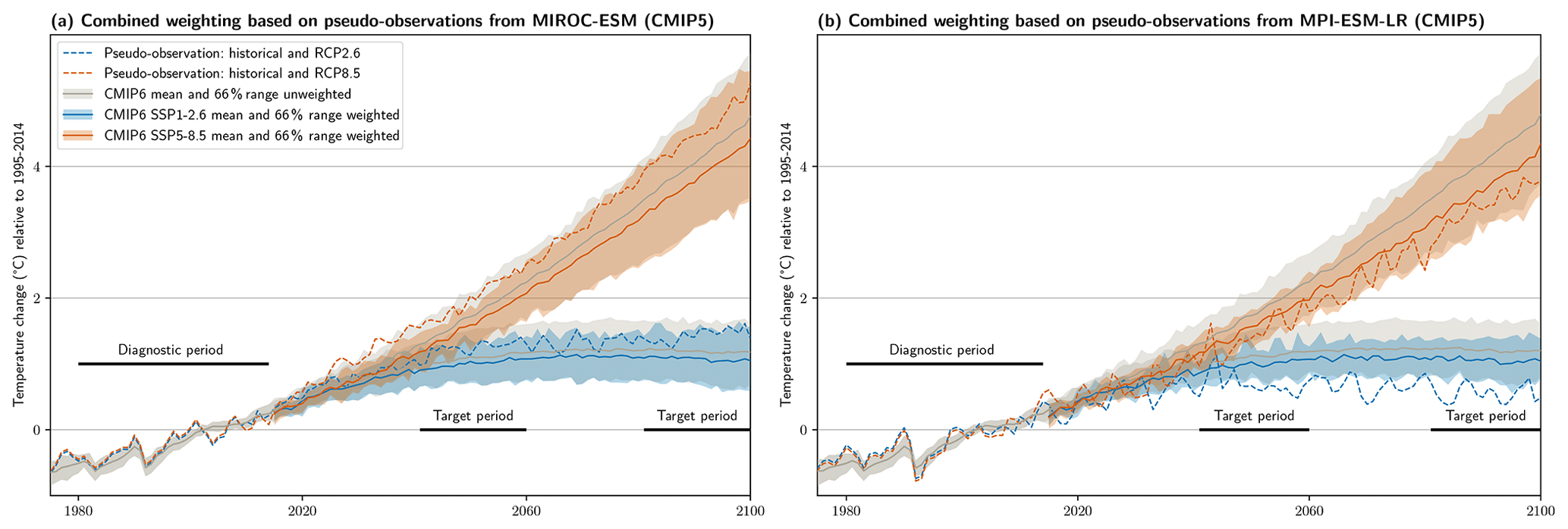
Figure 2Time series of temperature change (relative to 1995–2014) for the unweighted (gray) and weighted (colored) CMIP6 mean (lines) and likely (66 %) range (shading) as well as the CMIP5 models serving as pseudo-observations (dashed lines). Shown are the cases that lead to (a) the largest decrease in skill (CMIP5 pseudo-observation: MIROC-ESM) and (b) to the largest increase (MPI-ESM-LR) for SSP5-8.5 in the end-of-century target period. Note that no inference on the performance of the CMIP5 models can be drawn from this figure. The diagnostic period refers to the 1980–2014 period, which informs the weights; the target periods refer to 2041–2060 and 2081–2100.
The largest skill increases, in turn, often come from pseudo-observations rather far away from the unweighted mean. It seems that if the pseudo-observations behave very differently from the model ensemble in the historical period, there is a good chance that they will continue to do so in the future. One explanation for this could be a systematic difference between the models in the ensemble and the pseudo-observation due to factors such as a missing feedback or component. Thus, an important cautionary takeaway is to not only maximize the mean skill increase when setting up the method, as the cases with the highest skill might come from rather “unrealistic” pseudo-observations (i.e., those on the tails of the model distribution). This is illustrated in Fig. S5 (e.g., using the CMIP5 GFDL or GISS models as pseudo-observations). However, in many cases, we do not necessarily expect the real climate to follow such an extreme trajectory but rather to be closer to the unweighted MME mean (in part because real observations tend to be used in model development and tuning). Therefore, it is important to use a balanced set of multiple diagnostics and not only to optimize for maximal correlation when choosing σD, which might make the highest possible skill increases unattainable, but – maybe more importantly – to guard against even more substantial skill decreases.
Finally, it is important to note that the skill of the weighting for a given pseudo-observation also depends on the target. In isolated cases this can mean that the weighting leads to an increase in skill for one SSP while it leads to a decrease in the other (e.g., IPSL-CM5A-LR as pseudo-observation) or to an increase in one time period and to a decrease in the other (e.g., CSIRO-Mk3-6-0). An overview of the weighting based on each of the 27 CMIP5 models can be found in Fig. S5.

Figure 3(a) Similar to Fig. 1 but using 27 CMIP5 models as pseudo-observations and showing only the 50 % tasTREND case. (b) Map of the median of the CRPSS relative to the unweighted ensemble for 2041–2060 under SSP5-8.5.
To look into the skill change more quantitatively, Fig. 3a shows the skill distribution of weighting CMIP6 to predict each of the pseudo-observations drawn from CMIP5 for both target time periods and scenarios. We note again that for each CMIP5 pseudo-observation, the directly related CMIP6 models are excluded (see Table S5 for a list). Compared with the leave-one-out perfect model test with CMIP6 shown in Fig. 1, the increase in median CRPSS is lower and the risk of negative CRPSSs is slightly higher. This is not unexpected for a test sample that is structurally different from CMIP6 in several aspects (such as the forcing scheme and maximum amount of warming). However, the setup still achieves a median CRPSS increase of about 12 % to 22 %, with the risk of a skill reduction being confined to about 15 % of cases and to a maximum decrease of about 25 %. This clearly shows that ClimWIP can be used to provide reliable estimates of future global temperature change and related uncertainties from the CMIP6 MME.
Finally, we consider the question of whether there are regional patterns in the skill change by investigating a map of median CRPSSs for SSP5-8.5 in the mid-century period in Fig. 3b (see Fig. S6 for the other cases). Note that each CMIP6 model is still assigned only one weight, but the CRPSS is calculated at each respective grid point. The skill increases almost everywhere with the Northern Hemisphere having a slightly higher amplitude. A notable exception is the North Atlantic, where weighting leads to a slight decrease in the median skill. Indeed, this is the only region where the unweighted CMIP6 mean underestimates the warming from CMIP5. Weighting the CMIP6 ensemble leads to a slight strengthening of the underestimation in this region, whereas it reduces the difference almost everywhere else.

Figure 4Combined independence–performance weights for each CMIP6 model (line with dots) as well as pure performance weights (squares) and pure independence weights (triangles). All three cases are individually normalized, and the equal weighting each model would receive in a normal arithmetic mean is shown for reference (dashed line). The labels are colored by each model's TCR value: >2.5 ∘C – red, >2 ∘C – yellow, >1.5 ∘C – green, and ≤1.5 ∘C – blue. The number of ensemble members per model is shown in parentheses after the model name.
In summary, weighting CMIP6 in a perfect model test using five different diagnostics to establish model performance and two diagnostics for independence shows a clear increase in median skill compared with the unweighted distribution consistent over both investigated scenarios and time periods. Looking into the geographical distribution reveals an increase in skill almost everywhere, with some decreases found in the Southern Ocean, particularly in SSP1-2.6 (Fig. S6). Importantly, skill increases almost everywhere over land, thereby benefiting assessments of climate impacts and adaptation where people are affected most directly.
So far we have selected a combination of diagnostics that leads to the highest increase in median skill while minimizing the risk of a skill decrease based on an out-of-sample perfect model test with CMIP6 in Sect. 3.1. We also argued that we use the same shape parameters (which determine the strength of the weighting) for all cases, namely σS=0.54 for independence and σD=0.43 for performance. In Sect. 3.2, we then evaluated this setup using 27 pseudo-observations drawn from the CMIP5 MME. In this section, we now calculate weights for CMIP6 based on observed climate and validate the effect of the independence weighting. We use observational surface air temperature and sea level pressure estimates from the ERA5 and MERRA-2 reanalyses to calculate the performance diagnostics (tasANOM, tasSTD, tasTREND, pslANOM, and pslSTD). We continue to use model–model distances in tasCLIM and pslCLIM as independence diagnostics.
4.1 Calculation of weights for CMIP6
Figure 4 shows the combined performance and independence weights assigned to each CMIP6 model by ClimWIP when applied to the target of global temperature change. In addition, the individual performance and independence weights are also shown. All three cases are individually normalized. Applying the combined weight, about half of the models receive more weight than in a simple arithmetic mean and about half receive less. The best performing model, GFDL-ESM4, has about 4 times more influence than it would have without weighting (about 0.13 compared with 0.03 in the case with equal weighting). The three worst performing models, MIROC-ES2L, CanESM5, and HadGEM3-GC31-LL, in turn, receive less than 1∕20 of the equal weighting (about 0.001).
Indeed, several recent studies have found that models which show more future warming per unit of greenhouse gas are less likely based on comparison with past observations (e.g., Jiménez-de-la Cuesta and Mauritsen, 2019; Nijsse et al., 2020; Tokarska et al., 2020). Consistent with their findings, models with high TCR receive very low performance (and combined) weights (label colors in Fig. 4). Among the five lowest ranking models, four have a TCR above 2.5 ∘C, and all models with a TCR above 2.5 ∘C receive less then equal weight. The eight highest ranking models, in turn, have TCR values ranging from 1.5 to 2.5 ∘C; therefore, the lie in the middle of the CMIP6 TCR range. See Table S2 for a summary of all model weights and TCR values.
In addition to the combined weighting, Fig. 4 also shows the independence and performance weights separately. We discuss model independence in more detail in the next section. For the model performance weighting, the relative difference from the combined weighting (i.e., the influence of the independence weighting) is mostly below 50 %, with the MIROC model family being one notable exception. Both MIROC models are very independent, which shifts MIROC6 from a below-average model (based on the pure performance weight; square in Fig. 4) to an above-average model in the combined weight (dot in Fig. 4), effectively more than doubling its performance weight. For MIROC-ES2L the scaling due to independence is similarly high, but its total weight is still dominated by the very low performance weight. In the next section, we investigate if these independence weights indeed correctly represent the complex model interdependencies in the CMIP6 MME and appropriately down-weight models that are highly dependent on other models.
4.2 Validation of the independence weighting
Focusing on the independence weights in Fig. 4, one can broadly distinguish three cases: (i) relatively independent models, (ii) clusters of models that are quite dependent, and (iii) models for which the independence weighting does not really influence the weighting. To visualize and discuss these cases somewhat quantitatively, we show a CMIP6 model family tree similar to the work by Masson and Knutti (2011) and Knutti et al. (2013).
Using the same two diagnostics, namely horizontally resolved global temperature and sea level pressure climatologies (from 1980 to 2014), we apply a hierarchical clustering approach (Sect. 2.7). Figure 5 shows the resulting family tree of CMIP6 models similar to the work by Masson and Knutti (2011) and Knutti et al. (2013). In this tree, models that are closely related branch further to the left, whereas very independent model clusters branch further to the right. The mean generalized distance between two initial-condition members of the same model is used as an estimation of the internal variability and is indicated using gray shading. Models that have a distance similar to this value (e.g., the two CanESM5 model versions) are basically indistinguishable. The independence shape parameter used through the paper (σS=0.54) is shown as dashed vertical line.
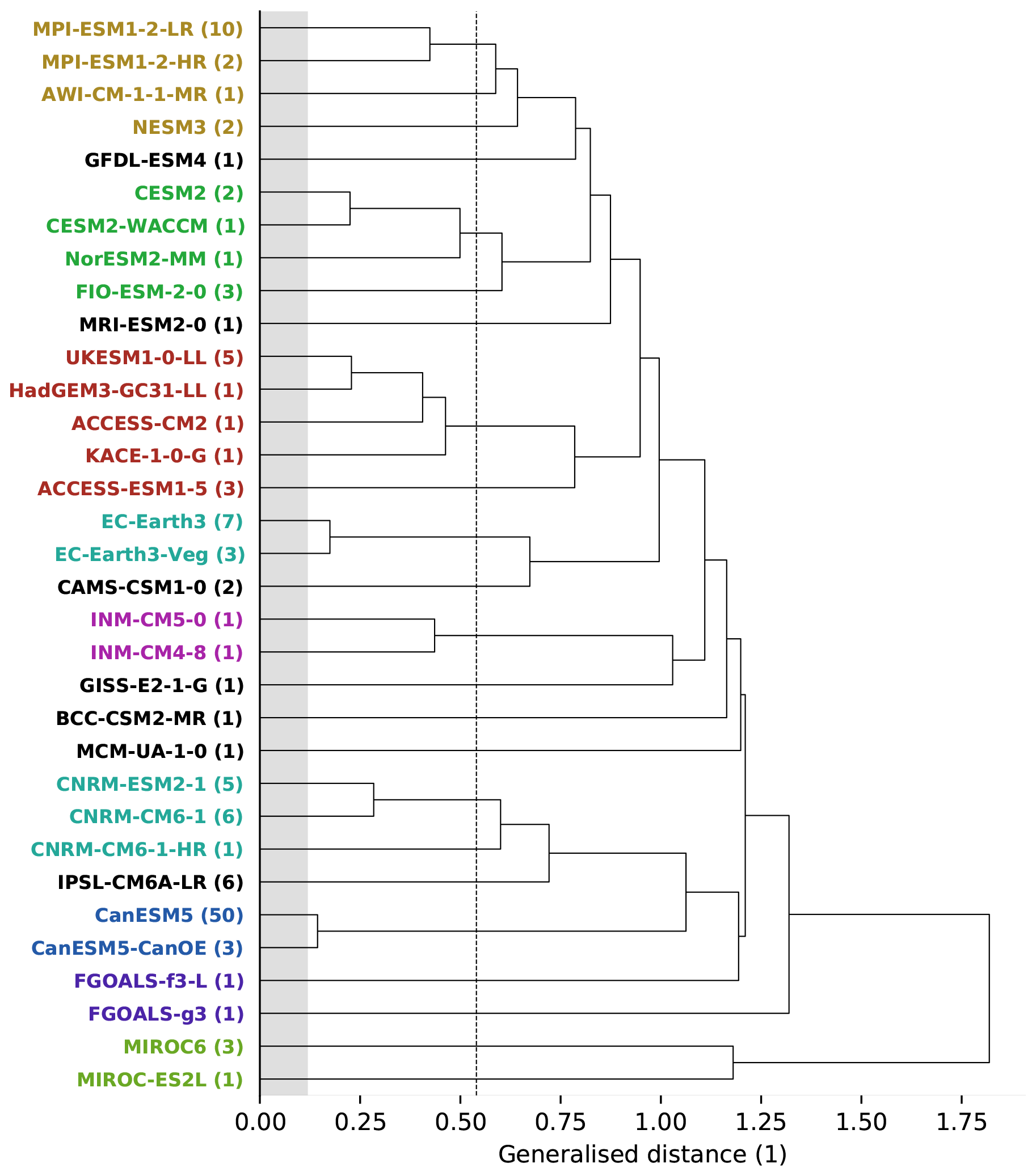
Figure 5Model family tree for all 33 CMIP6 models used in this study, similar to Knutti et al. (2013). Models branching further to the left are more dependent, and models branching further to the right are more independent. The analysis is based on global, horizontally resolved tasCLIM and pslCLIM in the period from 1980 to 2014. The independence shape parameter σS is indicated as dashed vertical line, and an estimation of internal variability is given using gray shading. Labels with the same color indicate models with obvious dependencies, such as shared components or the same origin, whereas models with no clear dependencies are labeled in black.
A comprehensive investigation of the complex interdependencies within the multi-model ensemble in use and further between models from the same institution or of similar origin is beyond the scope of this study and will be the subject of future work. Here, we limit ourselves to pointing out several base features of the output-based clustering, which serve as indications that it is skillful with respect to identifying interdependent models. The labels of models with the same origin or with known shared components are marked in the same color in Fig. 5. These two factors are the most objective measure for a priori model dependence that we have. The information about the model components is taken from each model's description page on the ES-DOC explorer (https://es-doc.org/cmip6/, last access: 17 April 2020), as listed in Table S4.
Figure 5 clearly shows that clustering models based on the selected diagnostics performs well: models with shared components or with the same origin (indicated by the same color) are always grouped together. Examining this in more detail, we find, for example, that closely related models such as low- and high-resolution versions (MPI-ESM-2-LR and MPI-ESM-2-HR; CNRM-CM6-1 and CNRM-CM6-1-HR) or versions with only one differing component (CESM2 and CESM2-WACCM; INM-CM5-0 and INM-CM4-8; both differing only in the atmosphere) are detected as being very similar. Both MIROC models, which have been identified as very independent based on Fig. 4, in turn, are found to be very far away from each other and even further away from all of the other models in the CMIP6 MME.
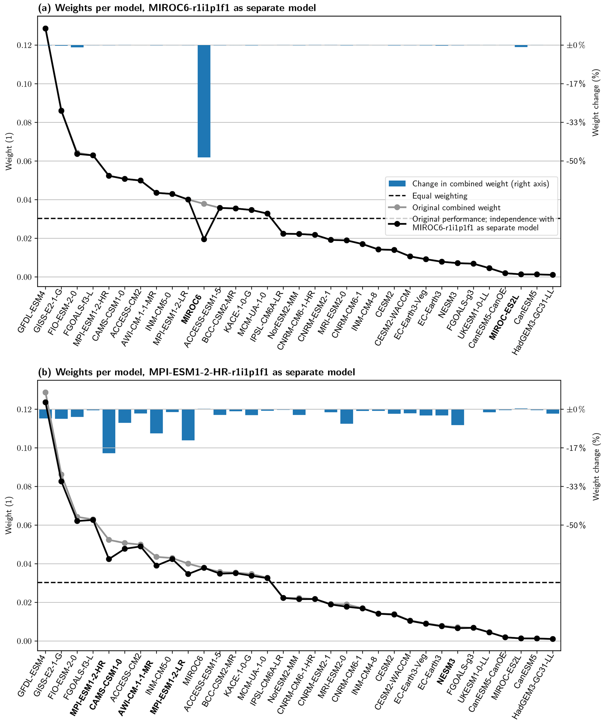
Figure 6Similar to Fig. 4 but removing one initial-condition ensemble member from (a) MIROC6 and (b) MPI-ESM1-2-HR and adding it as a separate model when calculating the independence weights (the “new” model is not shown in the plot). Models with obvious dependencies on the “new” model have bold labels (equivalent to Fig. 5). The change in the combined weight relative to the original weight is shown as blue bars using the right axis.
To investigate if the independence weighting correctly translates model distance into weights, we now look at two models as examples: one that performs well and is relatively independent (MIROC6) and another that also performs well but is more dependent (MPI-ESM1-2-HR). Each has multiple ensemble members; we remove one member from each and add it to the MME as an additional model, as detailed in Sect. 2.7.
In the first case (Fig. 6a; MIROC6 which is among the least dependent models), the original weight is reduced by almost half, which is close to what we would expect in the idealized case. All other models are unaffected by the addition of a duplicate of MIROC6, even the other model from the same center – MIROC-ES2L, which differs in atmospheric resolution and cumulus treatment (Tatebe et al., 2019; Hajima et al., 2020). Based on the “family tree” shown in Fig. 5 this behavior is not surprising: the two MIROC models are not only identified as the most independent models in the CMIP6 MME, but they are also identified as being very independent of one another. While some of the components and parameterizations are similar, updates to parameterizations and to the tuning of the parameters appear to be sufficient here to create a model that behaves quite differently.
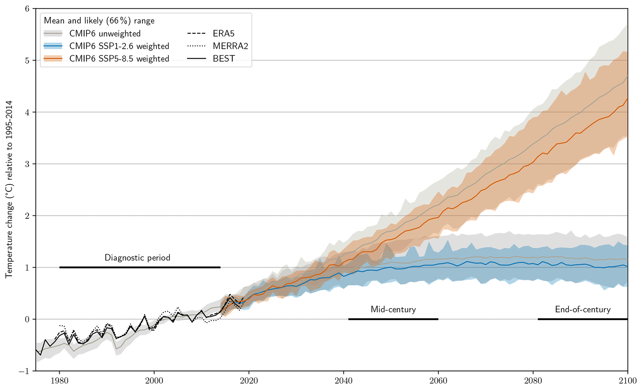
Figure 7Time series of temperature change (relative to 1995–2014) for the unweighted (gray) and weighted (colored) CMIP6 mean (lines) and likely (66 %) range (shading). Three observational datasets are also shown in black; note that BEST is not used to inform the weighting and is only shown for comparison here.
The second case (Fig. 6b; MPI-ESM1-2-HR which is among the most dependent models) shows a very different picture. The strongest effect on the original weight is found for the copied model itself, which is reduced by about 20 %, but several other models are also affected. Looking into these models in more detail, we conclude that the interdependencies detected by our method can be traced to shared components in most cases: MPI-ESM1-2-LR is just the low-resolution version of MPI-ESM1-2-HR (run with a T63 atmosphere instead of T127 and a 1.5∘ ocean instead of 0.4∘), AWI-CM-1-1-MR and NESM3 share the atmospheric component (ECHAM6.3) and have similar land (JSBACH3.x) components, and CAMS-CSM1-0 shares a similar atmospheric (ECHAM5) component. MRI-ESM2-0, in contrast, does not have any obvious dependencies. Information about the models can be found in their reference publications (Mauritsen et al., 2019; Gutjahr et al., 2019; Semmler et al., 2019; Yang et al., 2020; Chen et al., 2019; Yukimoto et al., 2019) and on the ES-DOC explorer, which provides detailed information about all of the models used in this study. The links to each model's information page can be found in Table S4.
4.3 Applying weights to CMIP6 temperature projections and TCR
Figure 7 shows a time series of unweighted and weighted projections based on a weak (SSP1-2.6) and strong (SSP5-8.5) climate change scenario. For both scenarios a clear shift in the mean towards less warming is visible, which is also reflected in the upper uncertainty bound. Notably, however, the lower bound hardly changes, leading to a general reduction in projection uncertainty. This becomes even clearer when investigating the two 20-year periods, reflecting mid- and end-of-century conditions (Fig. 8a and Table S3).

Figure 8(a) Unweighted (gray) and weighted (colors) temperature change (relative to 1995–2014) for both periods and scenarios. (b) Unweighted (gray) and weighted (green) transient climate response (TCR). The dots show individual models as labeled, with the size of the dot indicating the weight. The horizontal dot position is arbitrary.
Based on these results, warming exceeding 5 ∘C by the end of the century is very unlikely even under the strongest climate change scenario SSP5-8.5. The mean warming for this case is shifted downward to about 3.7 ∘C, and the 66 % (likely) and 90 % ranges are reduced by 13 % and 30 %, respectively. For SSP1-2.6 in the end-of-century period as well as both SSPs in the mid-century period, reductions in the mean warming of 0.1 to 0.2∘ C are found. The likely range is reduced by about 20 % to 35 % in these three cases. A summary of weights and warming values for all models as well as all statistics can be found in Tables S2 and S3. Recent studies that use the historical temperature trend as an observational constraint for future warming (e.g., Nijsse et al., 2020; Tokarska et al., 2020) lead to similar conclusions, with lower constrained warming compared with unconstrained (both in the mean and upper percentiles of the distributions).
To investigate the influence of remaining internal variability in our combination of diagnostics on the weighting, we also perform a bootstrap test. Selecting only one random member per model (for models with more than one ensemble member), we calculate weights and the corresponding unweighted and weighted temperature change distributions. This is repeated 100 times, providing uncertainty estimates for both the unweighted and weighted percentiles. The mean values of the weighted percentiles taken over all 100 bootstrap samples are very similar to the values from the weighting based on the full MME (including all ensemble members; see Fig. S7), confirming the robustness of our approach.
We also apply weights to TCR estimates in Fig. 8b, finding an unweighted mean TCR value of about 2 ∘C with a likely range of 1.6 to 2.5 ∘C. Weighting by historical model performance and independence constrains this to 1.9 ∘C (1.6 to 2.2 ∘C), which amounts to a reduction of 38 % in the likely range. These values are consistent with recent studies based on emergent constraints which estimate the likely range of TCR to be 1.3 to 2.1 ∘C (Nijsse et al., 2020) and 1.2 to 2.0 ∘C (Tokarska et al., 2020); they are also very similar to the range of 1.5 to 2.2 ∘C from Sherwood et al. (2020), who combined multiple lines of evidence. They are also consistent but substantially more narrow than the likely range from the Fifth Assessment Report of the Intergovernmental Panel on Climate Change (IPCC) (IPCC, 2013) based on CMIP5: 1 to 2.5 ∘C. Figure 8b clearly shows that almost all models with higher than equal weights lie within the likely range and only one model lies above it (FIO-ESM-2-0). This is a strong indication that TCR values beyond about 2.5 ∘C are unlikely when weighting based on several diagnostics and when accounting for model independence.
We have used the climate model weighting by independence and performance (ClimWIP) method to constrain projections of future global temperature change from the CMIP6 multi-model ensemble. Based on a leave-one-out perfect model test, a combination of five global, horizontally resolved diagnostic fields (anomaly, variance, and trend of surface air temperature, and anomaly and variance of sea level pressure) was selected to inform the performance weighting. The skill of weighting based on this selection was tested and confirmed in a second perfect model test using CMIP5 models as pseudo-observations. Our results clearly show the usefulness of this weighting approach in translating model spread into reliable estimates of future changes and, in particular, into uncertainties that are consistent with observations of present-day climate and observed trends.
We also discussed the remaining risk of decreasing skill compared with the raw distribution which is a crucial question in all weighting or constraining methods. We show the importance of using a balanced combination of climate system features (i.e., diagnostics) relevant for the target to inform the weighting in order to minimize the risk of skill decreases. This guards against the possibility of a model “accidentally” fitting observations for a single diagnostic while being far away from them in several others (and, hence, possibly not providing a skillful projection of the target variable).
By adding copies of existing models into the CMIP6 multi-model ensemble we verified the effect of the independence weighting, showing that models get correctly down-weighted based on an estimate of dependence derived from their output. To inform the independence weighting, we used two global, horizontally resolved fields (climatology of surface air temperature and sea level pressure) which we showed to allow a clear clustering of models with obvious interdependencies using a CMIP6 “family tree”.
From these tests, we conclude that ClimWIP is skillful in weighting global mean temperature change from CMIP6 using the selected setup. Hence, we use it to calculate weights for each CMIP6 model and apply them in order to obtain probabilistic estimates of future changes. Compared with the unweighted case, these results clearly show that the CMIP6 models that lead to the highest warming are less probable, confirming earlier studies (e.g., Nijsse et al., 2020; Sherwood et al., 2020; Tokarska et al., 2020). We find a weighted mean global temperature change (relative to 1995–2014) of 3.7 ∘C with a likely (66 %) range of 3.1 to 4.6 ∘C by the end of the century when following SSP5-8.5. With ambitious climate mitigation (SSP1-2.6) a weighted mean change of 1 ∘C (likely range from 0.7 to 1.4 ∘C) is projected for the same period.
On the policy level, this highlights the need for quick and decisive climate action to achieve the Paris climate targets. For climate modeling on the other hand, this approach demonstrates the potential to narrow the uncertainties in CMIP6 projections, particularly on the upper bound. The large investments in climate model development have not led to reduced model spread in the raw ensemble so far, but the use of climatological information and emergent transient constraints has the potential to provide more robust projections with reduced uncertainties, which are also more consistent with observed trends, thereby maximizing the value of climate model information for impacts and adaptation.
The ClimWIP model weighting package is available under a GNU General Public License, version 3 (GPLv3), at https://doi.org/10.5281/zenodo.4073039 (Brunner et al., 2020c).
The supplement related to this article is available online at: https://doi.org/10.5194/esd-11-995-2020-supplement.
LB, ALM, and RK were involved in conceiving the study. LB carried out the analysis and created the plots with substantial support from AGP. LB wrote the paper with contributions from all authors. The ClimWIP package was implemented by LB and RL. AGP wrote the script used to create Tables S4 and S6.
The authors declare that they have no conflict of interest.
The authors thank Martin B. Stolpe for providing the TCR values as well as Martin B. Stolpe and Katarzyna B. Tokarska for helpful discussions and comments on the paper. This work was carried out in the framework of the EUCP project, which is funded by the European Commission through the Horizon 2020 Research and Innovation program (grant agreement no. 776613). Ruth Lorenz was funded and Anna L. Merrifield was co-funded by the European Union's Horizon 2020 Research and Innovation program (grant agreement no. 641816; CRESCENDO). Flavio Lehner was supported by a SNSF Ambizione Fellowship (project no. PZ00P2_174128). This material is partly based upon work supported by the National Center for Atmospheric Research, which is a major facility sponsored by the National Science Foundation (NSF) under cooperative agreement no. 1947282, and by the Regional and Global Model Analysis (RGMA) component of the Earth and Environmental System Modeling Program of the U.S. Department of Energy's Office of Biological & Environmental Research (BER) via NSF IA no. 1844590. This study was generated using Copernicus Climate Change Service information 2020 from ERA5. The authors thank NASA for providing MERRA-2 and Berkeley Earth for providing BEST. We acknowledge the World Climate Research Programme, which, through its Working Group on Coupled Modelling, coordinated and promoted CMIP5 and CMIP6. We thank the climate modeling groups for producing and making their model output available, the Earth System Grid Federation (ESGF) for archiving the data and providing access, and the multiple funding agencies that support CMIP5, CMIP6, and ESGF. A list of all CMIP6 runs and their references can be found in Table S6. We thank all contributors to the numerous open-source packages that were crucial for this work, in particular the xarray Python project (http://xarray.pydata.org, v0.15.1). The authors thank the two anonymous reviewers for their helpful comments on our work.
This research has been supported by the H2020 European Research Council (grant no. EUCP 776613).
This paper was edited by Ben Kravitz and reviewed by two anonymous referees.
Abramowitz, G. and Bishop, C. H.: Climate model dependence and the ensemble dependence transformation of CMIP projections, J. Climate, 28, 2332–2348, https://doi.org/10.1175/JCLI-D-14-00364.1, 2015. a
Abramowitz, G., Herger, N., Gutmann, E., Hammerling, D., Knutti, R., Leduc, M., Lorenz, R., Pincus, R., and Schmidt, G. A.: ESD Reviews: Model dependence in multi-model climate ensembles: weighting, sub-selection and out-of-sample testing, Earth Syst. Dynam., 10, 91–105, https://doi.org/10.5194/esd-10-91-2019, 2019. a
Amos, M., Young, P. J., Hosking, J. S., Lamarque, J.-F., Abraham, N. L., Akiyoshi, H., Archibald, A. T., Bekki, S., Deushi, M., Jöckel, P., Kinnison, D., Kirner, O., Kunze, M., Marchand, M., Plummer, D. A., Saint-Martin, D., Sudo, K., Tilmes, S., and Yamashita, Y.: Projecting ozone hole recovery using an ensemble of chemistry–climate models weighted by model performance and independence, Atmos. Chem. Phys., 20, 9961–9977, https://doi.org/10.5194/acp-20-9961-2020, 2020. a
Andrews, T., Andrews, M. B., Bodas-Salcedo, A., Jones, G. S., Kuhlbrodt, T., Manners, J., Menary, M. B., Ridley, J., Ringer, M. A., Sellar, A. A., Senior, C. A., and Tang, Y.: Forcings, Feedbacks, and Climate Sensitivity in HadGEM3-GC3.1 and UKESM1, J. Adv. Model. Earth Syst., 11, 4377–4394, https://doi.org/10.1029/2019MS001866, 2019. a
Annan, J. D. and Hargreaves, J. C.: On the meaning of independence in climate science, Earth Syst. Dynam., 8, 211–224, https://doi.org/10.5194/esd-8-211-2017, 2017. a
Bishop, C. H. and Abramowitz, G.: Climate model dependence and the replicate Earth paradigm, Clim. Dynam., 41, 885–900, https://doi.org/10.1007/s00382-012-1610-y, 2013. a, b
Boé, J.: Interdependency in Multimodel Climate Projections: Component Replication and Result Similarity, Geophys. Res. Lett., 45, 2771–2779, https://doi.org/10.1002/2017GL076829, 2018. a, b, c
Boé, J. and Terray, L.: Can metric-based approaches really improve multi-model climate projections? The case of summer temperature change in France, Clim. Dynam., 45, 1913–1928, https://doi.org/10.1007/s00382-014-2445-5, 2015. a, b
Brunner, L., Lorenz, R., Zumwald, M., and Knutti, R.: Quantifying uncertainty in European climate projections using combined performance-independence weighting, Environ. Res. Lett., 14, 124010, https://doi.org/10.1088/1748-9326/ab492f, 2019. a, b, c, d, e, f, g, h
Brunner, L., Hauser, M., Lorenz, R., and Beyerle, U.: The ETH Zurich CMIP6 next generation archive: technical documentation, Zenodo, https://doi.org/10.5281/zenodo.3734128, 2020a. a
Brunner, L., McSweeney, C., Ballinger, A. P., Hegerl, G. C., Befort, D. J., O'Reilly, C., Benassi, M., Booth, B., Harris, G., Lowe, J., Coppola, E., Nogherotto, R., Knutti, R., Lenderink, G., de Vries, H., Qasmi, S., Ribes, A., Stocchi, P., and Undorf, S.: Comparing methods to constrain future European climate projections using a consistent framework, J. Climate, 33, 8671–8692, https://doi.org/10.1175/jcli-d-19-0953.1, 2020b. a, b
Brunner, L., Lorenz, R., Merrifield, A. L., and Sedlacek, J.: Climate model Weighting by Independence and Performance (ClimWIP): Code Freeze for Brunner et al. (2020) ESD, Zenodo, https://doi.org/10.5281/zenodo.4073039, 2020. a
Chen, X., Guo, Z., Zhou, T., Li, J., Rong, X., Xin, Y., Chen, H., and Su, J.: Climate Sensitivity and Feedbacks of a New Coupled Model CAMS-CSM to Idealized CO2 Forcing: A Comparison with CMIP5 Models, J. Meteorol. Res., 33, 31–45, https://doi.org/10.1007/s13351-019-8074-5, 2019. a
Cowtan, K.: The Climate Data Guide: Global surface temperatures: BEST: Berkeley Earth Surface Temperatures, available at: https://climatedataguide.ucar.edu/climate-data/global-surface-, last access: 9 September 2019. a
C3S: ERA5: Fifth generation of ECMWF atmospheric reanalyses of the global climate, https://doi.org/10.24381/cds.f17050d7, 2017. a
Deser, C., Phillips, A., Bourdette, V., and Teng, H.: Uncertainty in climate change projections: the role of internal variability, Clim. Dynam., 38, 527–546, https://doi.org/10.1007/s00382-010-0977-x, 2012. a
Eyring, V., Bony, S., Meehl, G. A., Senior, C. A., Stevens, B., Stouffer, R. J., and Taylor, K. E.: Overview of the Coupled Model Intercomparison Project Phase 6 (CMIP6) experimental design and organization, Geosci. Model Dev., 9, 1937–1958, https://doi.org/10.5194/gmd-9-1937-2016, 2016. a
Eyring, V., Cox, P. M., Flato, G. M., Gleckler, P. J., Abramowitz, G., Caldwell, P., Collins, W. D., Gier, B. K., Hall, A. D., Hoffman, F. M., Hurtt, G. C., Jahn, A., Jones, C. D., Klein, S. A., Krasting, J. P., Kwiatkowski, L., Lorenz, R., Maloney, E., Meehl, G. A., Pendergrass, A. G., Pincus, R., Ruane, A. C., Russell, J. L., Sanderson, B. M., Santer, B. D., Sherwood, S. C., Simpson, I. R., Stouffer, R. J., and Williamson, M. S.: Taking climate model evaluation to the next level, Nat. Clim. Change, 9, 102–110, https://doi.org/10.1038/s41558-018-0355-y, 2019. a
Flato, G., Marotzke, J., Abiodun, B., Braconnot, P., Chou, S., Collins, W., Cox, P., Driouech, F., Emori, S., Eyring, V., Forest, C., Gleckler, P., Guilyardi, E., Jakob, C., Kattsov, V., Reason, C., and Rummukainen, M.: Evaluation of Climate Models, in: Climate Change 2013: The Physical Science Basis, Contribution of Working Group I to the Fifth Assess- ment Report of the Intergovernmental Panel on Climate Change, edited by: Stocker, T., Qin, D., Plattner, G.-K., Tignor, M., Allen, S., Boschung, J., Nauels, A., Xia, Y., Bex, V., and Midgley, P., Cambridge University Press, Cambridge, UK and New York, NY, USA, 2013. a
Forster, P. M., Maycock, A. C., McKenna, C. M., and Smith, C. J.: Latest climate models confirm need for urgent mitigation, Nat. Clim. Change, 10, 7–10, https://doi.org/10.1038/s41558-019-0660-0, 2020. a, b
Gelaro, R., McCarty, W., Suárez, M. J., Todling, R., Molod, A., Takacs, L., Randles, C. A., Darmenov, A., Bosilovich, M. G., Reichle, R., Wargan, K., Coy, L., Cullather, R., Draper, C., Akella, S., Buchard, V., Conaty, A., da Silva, A. M., Gu, W., Kim, G. K., Koster, R., Lucchesi, R., Merkova, D., Nielsen, J. E., Partyka, G., Pawson, S., Putman, W., Rienecker, M., Schubert, S. D., Sienkiewicz, M., and Zhao, B.: The modern-era retrospective analysis for research and applications, version 2 (MERRA-2), J. Climate, 30, 5419–5454, https://doi.org/10.1175/JCLI-D-16-0758.1, 2017. a
Gettelman, A., Hannay, C., Bacmeister, J. T., Neale, R. B., Pendergrass, A. G., Danabasoglu, G., Lamarque, J., Fasullo, J. T., Bailey, D. A., Lawrence, D. M., and Mills, M. J.: High Climate Sensitivity in the Community Earth System Model Version 2 (CESM2), Geophys. Res. Lett., 46, 8329–8337, https://doi.org/10.1029/2019GL083978, 2019. a
Giorgi, F. and Coppola, E.: Does the model regional bias affect the projected regional climate change? An analysis of global model projections: A letter, Climatic Change, 100, 787–795, https://doi.org/10.1007/s10584-010-9864-z, 2010. a
Giorgi, F. and Mearns, L. O.: Calculation of average, uncertainty range, and reliability of regional climate changes from AOGCM simulations via the “Reliability Ensemble Averaging” (REA) method, J. Climate, 15, 1141–1158, https://doi.org/10.1175/1520-0442(2002)015<1141:COAURA>2.0.CO;2, 2002. a, b
Gleckler, P. J., Taylor, K. E., and Doutriaux, C.: Performance metrics for climate models, J. Geophys. Res. Atmos., 113, 1–20, https://doi.org/10.1029/2007JD008972, 2008. a
GMAO: MERRA-2 tavg1_2d_slv_Nx: 2d,1-Hourly,Time-Averaged,Single-Level,Assimilation,Single-Level Diagnostics V5.12.4, available at: https://disc.gsfc.nasa.gov/api/jobs/results/ 5e7b68e9ed720b5795af914a (last access: 25 March 2020), 2015a. a
GMAO: MERRA-2 statD_2d_slv_Nx: 2d,Daily,Aggregated Statistics,Single-Level,Assimilation,Single-Level Diagnostics V5.12.4, available at: https://disc.gsfc.nasa.gov/api/jobs/results/ 5e7b648f4900ab500326d17e (last access: 25 March 2020), 2015b. a
Golaz, J. C., Caldwell, P. M., Van Roekel, L. P., Petersen, M. R., Tang, Q., Wolfe, J. D., Abeshu, G., Anantharaj, V., Asay-Davis, X. S., Bader, D. C., Baldwin, S. A., Bisht, G., Bogenschutz, P. A., Branstetter, M., Brunke, M. A., Brus, S. R., Burrows, S. M., Cameron-Smith, P. J., Donahue, A. S., Deakin, M., Easter, R. C., Evans, K. J., Feng, Y., Flanner, M., Foucar, J. G., Fyke, J. G., Griffin, B. M., Hannay, C., Harrop, B. E., Hoffman, M. J., Hunke, E. C., Jacob, R. L., Jacobsen, D. W., Jeffery, N., Jones, P. W., Keen, N. D., Klein, S. A., Larson, V. E., Leung, L. R., Li, H. Y., Lin, W., Lipscomb, W. H., Ma, P. L., Mahajan, S., Maltrud, M. E., Mametjanov, A., McClean, J. L., McCoy, R. B., Neale, R. B., Price, S. F., Qian, Y., Rasch, P. J., Reeves Eyre, J. E., Riley, W. J., Ringler, T. D., Roberts, A. F., Roesler, E. L., Salinger, A. G., Shaheen, Z., Shi, X., Singh, B., Tang, J., Taylor, M. A., Thornton, P. E., Turner, A. K., Veneziani, M., Wan, H., Wang, H., Wang, S., Williams, D. N., Wolfram, P. J., Worley, P. H., Xie, S., Yang, Y., Yoon, J. H., Zelinka, M. D., Zender, C. S., Zeng, X., Zhang, C., Zhang, K., Zhang, Y., Zheng, X., Zhou, T., and Zhu, Q.: The DOE E3SM Coupled Model Version 1: Overview and Evaluation at Standard Resolution, J. Adv. Model. Earth Syst., 11, 2089–2129, https://doi.org/10.1029/2018MS001603, 2019. a
Gutjahr, O., Putrasahan, D., Lohmann, K., Jungclaus, J. H., Von Storch, J. S., Brüggemann, N., Haak, H., and Stössel, A.: Max Planck Institute Earth System Model (MPI-ESM1.2) for the High-Resolution Model Intercomparison Project (HighResMIP), Geosci. Model Dev., 12, 3241–3281, https://doi.org/10.5194/gmd-12-3241-2019, 2019. a
Hajima, T., Watanabe, M., Yamamoto, A., Tatebe, H., Noguchi, M. A., Abe, M., Ohgaito, R., Ito, A., Yamazaki, D., Okajima, H., Ito, A., Takata, K., Ogochi, K., Watanabe, S., and Kawamiya, M.: Development of the MIROC-ES2L Earth system model and the evaluation of biogeochemical processes and feedbacks, Geosci. Model Dev., 13, 2197–2244, https://doi.org/10.5194/gmd-13-2197-2020, 2020. a
Hawkins, E. and Sutton, R.: The Potential to Narrow Uncertainty in Regional Climate Predictions, B. Am. Meteorol. Soc., 90, 1095–1108, https://doi.org/10.1175/2009BAMS2607.1, 2009. a, b
Herger, N., Abramowitz, G., Knutti, R., Angélil, O., Lehmann, K., and Sanderson, B. M.: Selecting a climate model subset to optimise key ensemble properties, Earth Syst. Dynam., 9, 135–151, https://doi.org/10.5194/esd-9-135-2018, 2018a. a, b
Herger, N., Angélil, O., Abramowitz, G., Donat, M., Stone, D., and Lehmann, K.: Calibrating Climate Model Ensembles for Assessing Extremes in a Changing Climate, J. Geophys. Res.-Atmos., 123, 5988–6004, https://doi.org/10.1029/2018JD028549, 2018b. a
Hersbach, H.: Decomposition of the Continuous Ranked Probability Score for Ensemble Prediction Systems, Weather Forecast., 15, 559–570, https://doi.org/10.1175/1520-0434(2000)015<0559:DOTCRP>2.0.CO;2, 2000. a
IPCC: Climate Change 2013: The Physical Science Basis, in: Contribution of Working Group I to the Fifth Assessment Report of the Intergovern- mental Panel on Climate Change, Cambridge University Press, Cambridge, 2013. a
Jiménez-de-la Cuesta, D. and Mauritsen, T.: Emergent constraints on Earth's transient and equilibrium response to doubled CO2 from post-1970s global warming, Nat. Geosc., 12, 902–905, https://doi.org/10.1038/s41561-019-0463-y, 2019. a, b
Kay, J. E., Deser, C., Phillips, A., Mai, A., Hannay, C., Strand, G., Arblaster, J. M., Bates, S. C., Danabasoglu, G., Edwards, J., Holland, M., Kushner, P., Lamarque, J. F., Lawrence, D., Lindsay, K., Middleton, A., Munoz, E., Neale, R., Oleson, K., Polvani, L., and Vertenstein, M.: The community earth system model (CESM) large ensemble project: A community resource for studying climate change in the presence of internal climate variability, B. Am. Meteorol. Soc., 96, 1333–1349, https://doi.org/10.1175/BAMS-D-13-00255.1, 2015. a, b
Knutti, R.: The end of model democracy?, Climatic Change, 102, 395–404, https://doi.org/10.1007/s10584-010-9800-2, 2010. a
Knutti, R., Furrer, R., Tebaldi, C., Cermak, J., and Meehl, G. A.: Challenges in combining projections from multiple climate models, J. Climate, 23, 2739–2758, https://doi.org/10.1175/2009JCLI3361.1, 2010. a, b
Knutti, R., Masson, D., and Gettelman, A.: Climate model genealogy: Generation CMIP5 and how we got there, Geophys. Res. Lett., 40, 1194–1199, https://doi.org/10.1002/grl.50256, 2013. a, b, c, d, e, f, g, h
Knutti, R., Rugenstein, M. A., and Hegerl, G. C.: Beyond equilibrium climate sensitivity, Nat. Geosci., 10, 727–736, https://doi.org/10.1038/NGEO3017, 2017a. a
Knutti, R., Sedláček, J., Sanderson, B. M., Lorenz, R., Fischer, E. M., and Eyring, V.: A climate model projection weighting scheme accounting for performance and interdependence, Geophys. Res. Lett., 44, 1909–1918, https://doi.org/10.1002/2016GL072012, 2017b. a, b, c, d, e, f, g
Leduc, M., Laprise, R., de Elía, R., and Šeparović, L.: Is institutional democracy a good proxy for model independence?, J. Climate, 29, 8301–8316, https://doi.org/10.1175/JCLI-D-15-0761.1, 2016. a
Lehner, F., Deser, C., Maher, N., Marotzke, J., Fischer, E. M., Brunner, L., Knutti, R., and Hawkins, E.: Partitioning climate projection uncertainty with multiple large ensembles and CMIP5/6, Earth Syst. Dynam., 11, 491–508, https://doi.org/10.5194/esd-11-491-2020, 2020. a
Liang, Y., Gillett, N. P., and Monahan, A. H.: Climate Model Projections of 21st Century Global Warming Constrained Using the Observed Warming Trend, Geophys. Res. Lett., 47, 1–10, https://doi.org/10.1029/2019GL086757, 2020. a, b
Lorenz, R., Herger, N., Sedláček, J., Eyring, V., Fischer, E. M., and Knutti, R.: Prospects and Caveats of Weighting Climate Models for Summer Maximum Temperature Projections Over North America, J. Geophys. Res.-Atmos., 123, 4509–4526, https://doi.org/10.1029/2017JD027992, 2018. a, b, c, d, e, f
Maher, N., Milinski, S., Suarez-Gutierrez, L., Botzet, M., Dobrynin, M., Kornblueh, L., Kröer, J., Takano, Y., Ghosh, R., Hedemann, C., Li, C., Li, H., Manzini, E., Notz, D., Putrasahan, D., Boysen, L., Claussen, M., Ilyina, T., Olonscheck, D., Raddatz, T., Stevens, B., and Marotzke, J.: The Max Planck Institute Grand Ensemble: Enabling the Exploration of Climate System Variability, J. Adv. Model. Earth Syst., 11, 2050–2069, https://doi.org/10.1029/2019MS001639, 2019. a, b
Masson, D. and Knutti, R.: Climate model genealogy, Geophys. Res. Lett., 38, 1–4, https://doi.org/10.1029/2011GL046864, 2011. a, b, c, d, e
Mauritsen, T., Bader, J., Becker, T., Behrens, J., Bittner, M., Brokopf, R., Brovkin, V., Claussen, M., Crueger, T., Esch, M., Fast, I., Fiedler, S., Fläschner, D., Gayler, V., Giorgetta, M., Goll, D. S., Haak, H., Hagemann, S., Hedemann, C., Hohenegger, C., Ilyina, T., Jahns, T., Jimenéz-de-la Cuesta, D., Jungclaus, J., Kleinen, T., Kloster, S., Kracher, D., Kinne, S., Kleberg, D., Lasslop, G., Kornblueh, L., Marotzke, J., Matei, D., Meraner, K., Mikolajewicz, U., Modali, K., Möbis, B., Müller, W. A., Nabel, J. E., Nam, C. C., Notz, D., Nyawira, S. S., Paulsen, H., Peters, K., Pincus, R., Pohlmann, H., Pongratz, J., Popp, M., Raddatz, T. J., Rast, S., Redler, R., Reick, C. H., Rohrschneider, T., Schemann, V., Schmidt, H., Schnur, R., Schulzweida, U., Six, K. D., Stein, L., Stemmler, I., Stevens, B., von Storch, J. S., Tian, F., Voigt, A., Vrese, P., Wieners, K. H., Wilkenskjeld, S., Winkler, A., and Roeckner, E.: Developments in the MPI-M Earth System Model version 1.2 (MPI-ESM1.2) and Its Response to Increasing CO2, J. Adv. Model. Earth Syst., 11, 998–1038, https://doi.org/10.1029/2018MS001400, 2019. a
Merrifield, A. L., Brunner, L., Lorenz, R., Medhaug, I., and Knutti, R.: An investigation of weighting schemes suitable for incorporating large ensembles into multi-model ensembles, Earth Syst. Dynam., 11, 807–834, https://doi.org/10.5194/esd-11-807-2020, 2020. a, b, c, d, e, f, g, h
Müllner, D.: Modern hierarchical, agglomerative clustering algorithms, 1–29, arxiv preprint: http://arxiv.org/abs/1109.2378 (last access: 6 April 2020), 2011. a
Nijsse, F. J. M. M., Cox, P. M., and Williamson, M. S.: Emergent constraints on transient climate response (TCR) and equilibrium climate sensitivity (ECS) from historical warming in CMIP5 and CMIP6 models, Earth Syst. Dynam., 11, 737–750, https://doi.org/10.5194/esd-11-737-2020, 2020. a, b, c, d, e, f
O'Neill, B. C., Kriegler, E., Riahi, K., Ebi, K. L., Hallegatte, S., Carter, T. R., Mathur, R., and van Vuuren, D. P.: A new scenario framework for climate change research: the concept of shared socioeconomic pathways, Climatic Change, 122, 387–400, https://doi.org/10.1007/s10584-013-0905-2, 2014. a
Pennell, C. and Reichler, T.: On the Effective Number of Climate Models, J. Climate, 24, 2358–2367, https://doi.org/10.1175/2010JCLI3814.1, 2011. a
Ribes, A., Zwiers, F. W., Azaïs, J. M., and Naveau, P.: A new statistical approach to climate change detection and attribution, Clim. Dynam., 48, 367–386, https://doi.org/10.1007/s00382-016-3079-6, 2017. a
Sanderson, B. and Wehner, M.: Appendix B. Model Weighting Strategy, Forth Natl. Clim. Assess., 1, 436–442, https://doi.org/10.7930/J06T0JS3, 2017. a
Sanderson, B. M., Knutti, R., and Caldwell, P.: A representative democracy to reduce interdependency in a multimodel ensemble, J. Climate, 28, 5171–5194, https://doi.org/10.1175/JCLI-D-14-00362.1, 2015a. a
Sanderson, B. M., Knutti, R., and Caldwell, P.: Addressing interdependency in a multimodel ensemble by interpolation of model properties, J. Climate, 28, 5150–5170, https://doi.org/10.1175/JCLI-D-14-00361.1, 2015b. a
Sanderson, B. M., Wehner, M., and Knutti, R.: Skill and independence weighting for multi-model assessments, Geosci. Model Dev., 10, 2379–2395, https://doi.org/10.5194/gmd-10-2379-2017, 2017. a, b, c
Selten, F. M., Bintanja, R., Vautard, R., and van den Hurk, B. J.: Future continental summer warming constrained by the present-day seasonal cycle of surface hydrology, Scient. Rep., 10, 1–7, https://doi.org/10.1038/s41598-020-61721-9, 2020. a
Semmler, T., Danilov, S., Gierz, P., Goessling, H., Hegewald, J., Hinrichs, C., Koldunov, N. V., Khosravi, N., Mu, L., and Rackow, T.: Simulations for CMIP6 with the AWI climate model AWI-CM-1-1, Earth Space Science Open Archive, p. 48, https://doi.org/10.1002/essoar.10501538.1, 2019. a
Sherwood, S., Webb, M. J., Annan, J. D., Armour, K. C., Forster, P. M., Hargreaves, J. C., Hegerl, G., Klein, S. A., Marvel, K. D., Rohling, E. J., Watanabe, M., Andrews, T., Braconnot, P., Bretherton, C. S., Foster, G. L., Hausfather, Z., von der Heydt, A. S., Knutti, R., Mauritsen, T., Norris, J. R., Proistosescu, C., Rugenstein, M., Schmidt, G. A., Tokarska, K. B., and Zelinka, M. D.: An assessment of Earth's climate sensitivity using multiple lines of evidence, Rev. Geophys., 58, 4, https://doi.org/10.1029/2019rg000678, 2020. a, b
Swart, N. C., Cole, J. N., Kharin, V. V., Lazare, M., Scinocca, J. F., Gillett, N. P., Anstey, J., Arora, V., Christian, J. R., Hanna, S., Jiao, Y., Lee, W. G., Majaess, F., Saenko, O. A., Seiler, C., Seinen, C., Shao, A., Sigmond, M., Solheim, L., Von Salzen, K., Yang, D., and Winter, B.: The Canadian Earth System Model version 5 (CanESM5.0.3), Geosci. Model Dev., 12, 4823–4873, https://doi.org/10.5194/gmd-12-4823-2019, 2019. a
Tatebe, H., Ogura, T., Nitta, T., Komuro, Y., Ogochi, K., Takemura, T., Sudo, K., Sekiguchi, M., Abe, M., Saito, F., Chikira, M., Watanabe, S., Mori, M., Hirota, N., Kawatani, Y., Mochizuki, T., Yoshimura, K., Takata, K., O'Ishi, R., Yamazaki, D., Suzuki, T., Kurogi, M., Kataoka, T., Watanabe, M., and Kimoto, M.: Description and basic evaluation of simulated mean state, internal variability, and climate sensitivity in MIROC6, Geosci. Model Dev., 12, 2727–2765, https://doi.org/10.5194/gmd-12-2727-2019, 2019. a
Tebaldi, C. and Knutti, R.: The use of the multi-model ensemble in probabilistic climate projections, Philos. T. Roy. Soc. A, 365, 2053–2075, https://doi.org/10.1098/rsta.2007.2076, 2007. a
Tegegne, G., Kim, Y.-O., and Lee, J.-K.: Spatiotemporal reliability ensemble averaging of multi‐model simulations, Geophys. Res. Lett., 46, 12321–12330, https://doi.org/10.1029/2019GL083053, 2019. a
Tokarska, K. B., Stolpe, M. B., Sippel, S., Fischer, E. M., Smith, C. J., Lehner, F., and Knutti, R.: Past warming trend constrains future warming in CMIP6 models, Sci. Adv., 6, eaaz9549, https://doi.org/10.1126/sciadv.aaz9549, 2020. a, b, c, d, e, f, g
van Vuuren, D. P., Edmonds, J., Kainuma, M., Riahi, K., Thomson, A., Hibbard, K., Hurtt, G. C., Kram, T., Krey, V., Lamarque, J. F., Masui, T., Meinshausen, M., Nakicenovic, N., Smith, S. J., and Rose, S. K.: The representative concentration pathways: An overview, Climatic Change, 109, 5–31, https://doi.org/10.1007/s10584-011-0148-z, 2011. a
Voldoire, A., Saint‐Martin, D., Sénési, S., Decharme, B., Alias, A., Chevallier, M., Colin, J., Guérémy, J., Michou, M., Moine, M., Nabat, P., Roehrig, R., Salas y Mélia, D., Séférian, R., Valcke, S., Beau, I., Belamari, S., Berthet, S., Cassou, C., Cattiaux, J., Deshayes, J., Douville, H., Ethé, C., Franchistéguy, L., Geoffroy, O., Lévy, C., Madec, G., Meurdesoif, Y., Msadek, R., Ribes, A., Sanchez‐Gomez, E., Terray, L., and Waldman, R.: Evaluation of CMIP6 DECK Experiments With CNRM‐CM6‐1, J. Adv. Model. Earth Syst., 11, 2177–2213, https://doi.org/10.1029/2019MS001683, 2019. a
Yang, Y.-M., Wang, B., Cao, J., Ma, L., and Li, J.: Improved historical simulation by enhancing moist physical parameterizations in the climate system model NESM3.0, Clim. Dynam., 54, 3819–3840, https://doi.org/10.1007/s00382-020-05209-2, 2020. a
Yukimoto, S., Kawai, H., Koshiro, T., Oshima, N., Yoshida, K., Urakawa, S., Tsujino, H., Deushi, M., Tanaka, T., Hosaka, M., Yabu, S., Yoshimura, H., Shindo, E., Mizuta, R., Obata, A., Adachi, Y., and Ishii, M.: The meteorological research institute Earth system model version 2.0, MRI-ESM2.0: Description and basic evaluation of the physical component, J. Meteorol. Soc. Jpn., 97, 931–965, https://doi.org/10.2151/jmsj.2019-051, 2019. a
Zelinka, M. D., Myers, T. A., McCoy, D. T., Po‐Chedley, S., Caldwell, P. M., Ceppi, P., Klein, S. A., and Taylor, K. E.: Causes of Higher Climate Sensitivity in CMIP6 Models, Geophys. Res. Lett., 47, 1–12, https://doi.org/10.1029/2019GL085782, 2020. a, b
- Abstract
- Introduction
- Data and methods
- Evaluation of the weighting in the perfect model test
- Weighting CMIP6 projections of future warming based on observations
- Discussion and conclusions
- Code availability
- Author contributions
- Competing interests
- Acknowledgements
- Financial support
- Review statement
- References
- Supplement