the Creative Commons Attribution 4.0 License.
the Creative Commons Attribution 4.0 License.
 | 05 Jun 2020
On the interconnections among major climate modes and their common driving factors
Xinnong Pan
Geli Wang
Peicai Yang
Jun Wang
Anastasios A. Tsonis
The variations in oceanic and atmospheric modes on various timescales play
important roles in generating global and regional climate variability. Many
efforts have been devoted to identifying the relationships between the
variations in climate modes and regional climate variability, but these have rarely
explored the interconnections among these climate modes. Here we use climate
indices to represent the variations in major climate modes and examine the
harmonic relationship among the driving forces of climate modes using slow
feature analysis (SFA) and wavelet analysis. We find that all of the
significant peak periods of driving-force signals in the climate indices can
be represented as harmonics of four base periods: 2.32, 3.90, 6.55,
and 11.02 years. We infer that the period of 2.32 years is associated with the
signal of the quasi-biennial oscillation (QBO). The periods of 3.90 and 6.55 years are linked to the intrinsic variability of the El Niño–Southern
Oscillation (ENSO), and the period of 11.02 years arises from the sunspot
cycle. Results suggest that the base periods and their harmonic oscillations
related to QBO, ENSO, and solar activities act as key connections among the
climatic modes with synchronous behaviors, highlighting the important roles
of these three oscillations in the variability of the Earth's climate.
Highlights.
- i.
The harmonic relationship among the driving forces of climate modes was investigated by using slow feature analysis and wavelet analysis.
- ii.
All of the significant peak periods of driving-force signals in climate indices can be represented as the harmonics of four base periods.
- iii.
The four base periods related to QBO, ENSO, and solar activities act as the key linkages among different climatic modes with synchronous behaviors.
- Article
(2450 KB) - Full-text XML
-
Supplement
(594 KB) - BibTeX
- EndNote


The influences of large-scale climate modes (e.g., El Niño–Southern Oscillation (ENSO), Pacific Decadal Oscillation (PDO), North Atlantic Oscillation (NAO), and the Atlantic Multidecadal Oscillation – AMO) on the variations of global to regional climate (e.g., temperature, rainfall, and atmospheric circulations) have been extensively examined (Bradley et al., 1987; Wu et al., 2003; McCabe et al., 2004; Kenyon and Hegerl, 2008; Steinman et al., 2015; Wang et al., 2016, 2017; Yang et al., 2016; R. Zhang et al., 2017; Xie et al., 2019). It has been well established that regional climate variations at various temporal and spatial scales are modulated by the variabilities of major climate modes. For instance, Wu et al. (2003) estimated that about 25 % of rainfall variance in fall and winter over southern China can be explained by ENSO. McCabe et al. (2004) reported that the PDO and AMO have contributed to more than half (52 %) of the spatiotemporal variance in multidecadal drought occurrence over the conterminous United States. Xie et al. (2019) found that the multidecadal variability in East Asian surface air temperature (EASAT) is highly associated with the NAO, which leads detrended annual EASAT by 15–20 years. Based on this relationship, they proposed an NAO-based linear model to predict the near-future change in EASAT.
The variations of oceanic and atmospheric modes affect regional climate mainly through the teleconnections within the atmosphere (i.e., atmospheric bridge) and ocean (i.e., oceanic tunnel) (Liu and Alexander, 2007). Atmospheric teleconnections can be produced by both external forcings from ocean or land (e.g., sea surface temperature (SST) anomalies related to ENSO) and internal atmospheric processes (e.g., Rossby wave in the westerlies) (Trenberth et al., 1998). Though many theories have been developed to explain the physical mechanisms behind the influences of major climate modes on regional climate, the interconnections among these climate modes per se and their primary driving factors remain largely unclear. Given that remote teleconnections exist between climate modes and regional climate at various temporal and spatial scales, tight interconnections are expected to exist among these climate modes (Rossi et al., 2011). In addition, acting as the primary regulator of the energy budget of the climate system, the external forcings of climate system (e.g., solar activities) impose extensive influences on various climate modes (e.g., ENSO and NAO) (Kirov and Georgieva, 2002; Velasco and Mendoza, 2008). Thus, it appears to be promising to identify the interconnections among major climate modes and their common driving factors. As the indicators of climate modes, many climate indices (e.g., SST anomaly in the Niño 3.4 region for ENSO) have been proposed and widely used to investigate the dynamic processes and physical mechanisms within the climate system (Dai, 2006; Steinman et al., 2015; Wang et al., 2017). However, the major barrier to clarifying the interconnections of these climate indices is how to effectively extract the driving forces and identify their corresponding essential driving factors.
It is well recognized that most of the time series observed in the real world are nonstationary because of the effects of external perturbations (Verdes et al., 2001). Climate is in general a nonstationary dynamic system. As such, the driving forces in the variations of major climate modes remain difficult to determine. Some pioneering works have been conducted to overcome this daunting challenge. For example, Yang et al. (2003) proposed a physical conceptual framework within which the nonstationary features of the climate system are relevant to the characteristics of a hierarchical structure: the driving force originating from a higher-hierarchy subsystem controls the behaviors of a lower-hierarchy subsystem in a cascade way. Compared to the dynamic reality manifested in the lower-hierarchy subsystem, the driving force of the higher-hierarchy subsystem is a much slower process. In other words, the essential differences between higher and lower subsystems are reflected in scale and energy. Many efforts have been devoted to extracting information on driving forces from the dynamic system (Verdes et al., 2001; Wiskott et al., 2002; Yang et al., 2016). Slow feature analysis (SFA) is an algorithm that was developed to extract the slowly varying features from nonstationary time series, which provides a direct and effective approach to identify the driving forces of a nonstationary dynamic system. Based on idealized models (e.g., tent map and logistic map), recent studies have demonstrated that SFA can extract slowly varying driving forces and subcomponent signals from fast-varying nonstationary time series even without any prerequisite knowledge about the underlying dynamic system and its driving forces (Wiskott et al., 2002; Konen and Koch, 2011; Escalante-B and Wiskott, 2012).
Considering that the driving-force signal of a dynamic system often consists of different components with various timescales, Pan et al. (2017) robustly detected independent driving-force factors that contain significant peak periods from the SFA-extracted signals by combing SFA with wavelet analysis (Torrence and Compo, 1998). Recently, this kind of technique that combines the SFA with wavelet analysis has also been applied to detect the external and internal driving-force signals responsible for the variations of a regional climate, such as the drought variability in the southwestern United States (F. Zhang et al., 2017), the temperature variations in central England (Wang et al., 2017) and the Northern Hemisphere (Yang et al., 2016), and the oscillations of stratospheric ozone concentration (Wang et al., 2016). In this study, we employed this new approach to understand the interconnections among major climate modes and their primary driving factors. The remainder of this paper is organized as follows. The data and methods are described in Sects. 2 and 3, respectively. The main results are presented in Sect. 4, followed by the conclusions and a discussion in Sect. 5.
We use monthly mean indices to represent four widely investigated climate modes (ENSO, PDO, AMO, and NAO) that were developed and provided by NOAA (https://psl.noaa.gov/gcos_wgsp/Timeseries/, last access: 1 March 2020). Figure 1 shows the normalized series of these climate indices. These indices and their corresponding climate modes are described briefly as follows.
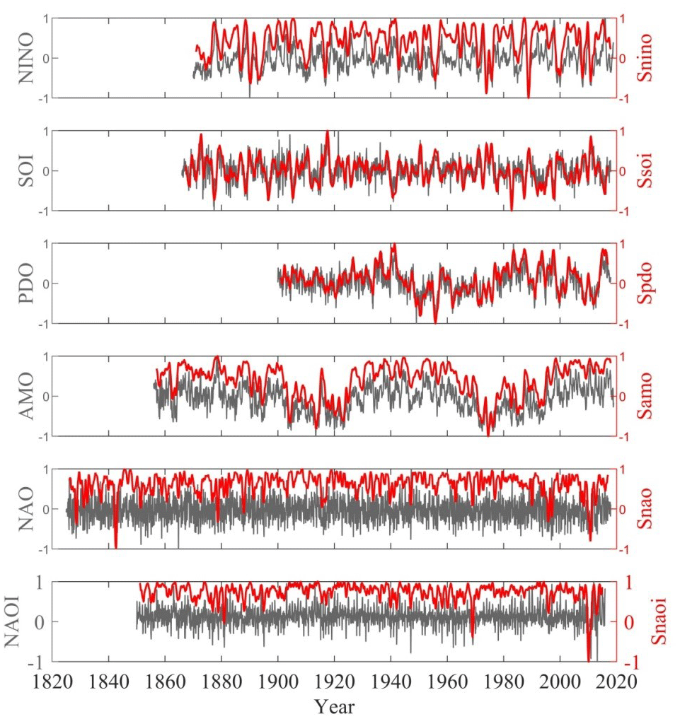
Figure 1Normalized monthly time series of six climate indices during each period (gray lines): NINO (01/1870–12/2018), SOI (01/1866–12/2017), PDO (01/1900–12/2017), AMO (01/1856–12/2018), NAO (01/1825–12/2017), and NAOI (01/1850–12/2015) with their corresponding SFA-derived slow feature signals (red lines), which are indicated by Snino, Ssoi, Spdo, Samo, Snao, and Snaoi, respectively (setting embedding dimension m to be 11).
2.1 ENSO
ENSO is well recognized as a natural ocean–atmosphere coupled mode in the tropical Pacific (Deser et al., 2010) affecting the global climate (Newman et al., 2003). El Niño (La Niña) refers to the warming (cooling) phase of the tropical Pacific Ocean occurring every 2–7 years. Meanwhile, the anomalous warming or cooling conditions are linked to a large-scale east–west seesaw air pressure pattern referred to as the Southern Oscillation (Capotondi et al., 2015). El Niño and the Southern Oscillation are two manifestations of the ENSO phenomenon (Bjerknes, 1969). In this study, ENSO is represented by both the Niño 3.4 index and the Southern Oscillation index (SOI). The Niño 3.4 index (1870/01–2018/12, hereafter referred to as NINO) is defined as the SST anomalies in the Niño 3.4 region (5∘ N–5∘ S; 170–120∘ W) based on the HadISST1 dataset (Rayner et al., 2003). The SOI (1866/01–2017/12) is calculated from the observed standardized sea level pressure (SLP) differences between the islands of Tahiti and Darwin, Australia (Ropelewski and Jones, 1987).
2.2 PDO
PDO is the dominant pattern of decadal variability in North Pacific SST, which has been widely studied across different disciplines (Newman et al., 2016). A previous study shows that the changing phase of PDO affects the anomalies of atmospheric circulation around the North Pacific Ocean basin and even the Southern Hemisphere (Mantua and Hare, 2002). The characteristic period of PDO is 50–60 years, and a warm or cold phase of PDO can typically persist for about 20–30 years. If PDO is in its positive phase, the North Pacific Ocean turns colder and the Middle East Pacific Ocean turns warmer; otherwise, it is in a negative phase. In this study, PDO is defined by the leading principal component of monthly SST anomalies in the Pacific basin (poleward of 20∘ N) during 1900–2017 (Mantua et al., 1997).
2.3 AMO
AMO is a dominant signal of climate variability in the North Atlantic SST, which has a statistically significant spectral peak in the 50–70-year band (Schlesinger and Ramankutty, 1994; Sun et al., 2015). Related studies have suggested that AMO is an inner variability of the climate system modulating hemispheric climate change (Zhang, 2007; Knight et al., 2006). The slow variation of the Atlantic meridional overturning circulation (AMOC) plays a dominant role in the Atlantic multidecadal variability of SST (Zhang, 2017; Delworth and Mann, 2000; Garuba et al., 2018). The AMO is defined by the detrended area-weighted average SST over the North Atlantic (from 0 to 70∘ N) during 1856–2018 based on the Kaplan SST dataset (Enfield et al., 2001). Both unsmoothed and smoothed AMO indexes are available. The high-frequency variability of the smoothed AMO index has been removed by a common 121-month filter. We choose to use the unsmoothed AMO index in this study.
2.4 NAO
The NAO is active in the North Atlantic region, which is characterized by a large-scale seesaw in atmospheric mass between the subtropical high and the polar low (Li and Wang, 2003). It manifests as climate fluctuations at multiple timescales ranging from interannual to multidecadal variabilities (Jones et al., 1997; Li et al., 2013), affecting the climate within and around the North Atlantic Ocean basin and even the entire Northern Hemisphere (Wallace and Gutzler, 1981; Hurrell, 1995; Li et al., 2013; Delworth et al., 2017; Jajcay et al., 2016). Although the climatic effect of the NAO is most pronounced in winter, it is the dominant mode of atmospheric circulation in the North Atlantic sector throughout the whole year. A previous study suggested that the NAO drives the North Atlantic SST anomalies at a timescale less than 10 years (Delworth et al., 2017). The NAO index is typically defined as a meridional dipole mode (which has lately been suggested to be a three-pole pattern; Tsonis et al., 2008) in atmospheric pressure with two centers of action in Iceland and the Azores during 1825–2017. For comparison, we also examine another observationally based monthly NAO index for the period 1850–2015 (hereafter referred to as NAOI), which is defined by the difference in the normalized sea level pressure (SLP) that is zonally averaged over the North Atlantic sector from 80∘ W to 30∘ E between 35 and 65∘ N (Li and Wang, 2003; http://ljp.gcess.cn/dct/page/65610, last access: 1 March 2020). The NAOI is calculated based on the HadSLP dataset with the reference period of 1961–1990.
3.1 Slow feature analysis (SFA)
Based on time-embedding theorems, one-dimensional time series can turn into a multidimensional system. For this multidimensional input system, the SFA acts as a nonlinear method that uses a nonlinear expansion to map the input signal into a feature space and solves a linear problem (Blaschke et al., 2006). The objective of SFA is to find instantaneous scalar input–output functions that generate output signals that vary as slowly as possible but still carry significant information. To ensure this, we require the output signals to be uncorrelated and have unit variance (Franzius et al., 2011).
Consider a time series , where t denotes time and n indicates the length of the time series. First, we embed {x(t)} into an m-dimensional state space:
where . Then nonlinear expansions (usually second-order polynomials) are used to generate a k-dimensional function state space:
which can also be written as , where
Then, the expanded signal H(t) is normalized so that it satisfies the constraints of zero mean and unit variance. This process is referred to as whitening or sphering. Thus, we have
Using the Schmidt algorithm, H′(t) is orthogonalized into
Thus, each output signal can be expressed as the following linear combination:
where is a set of weighting coefficients.
Note that the output signals are orthogonal and nontrivial:
Subsequently, we perform first-order differencing on Z(t) to obtain the derivative function space:
Then we calculate the time-derivative K×K covariance matrix , where its eigenvalues are and the corresponding eigenvectors are . Finally, using W1, the driving force can be written as
where r and c are two arbitrary constants that are derived from the quadrature of y(t) and the solution of W1, respectively.
3.2 Wavelet analysis
Wavelet analysis is widely used to analyze localized structures and spectral properties of time series. Torrence (1998) provided a useful tool kit to conduct wavelet analysis step by step, including a statistical significance test. The tool kit can be accessed from the following website: http://paos.colorado.edu/research/wavelets/ (last access: 1 March 2020).
In this study, we use the Morlet wavelet that offers a high spectrum resolution. The wavenumber is set to 4, representing a lower-resolution wavelet scale to analyze the time-averaged global power spectrum of climate indices. A previous study based on idealized models shows that the significant peak periods of the SFA-derived signal correspond well to the driving-force factors (Pan et al., 2017). Here we focus on the peak periods that are statistically significant at the 0.05 significance level.
As the first step, we set the embedding dimension m to 11 (within 1 year) for the SFA and extract each driving-force signal from six climate indices, which are denoted as Snino, Ssoi, Spdo, Samo, Snao, and Snaoi. Figure 1 shows the variations of these SFA-extracted driving-force signals (red lines) along with the native time series (gray lines) of climate indices. It should be noted that the slowly varying signals extracted by the SFA are essentially different from the low-frequency signal obtained by low-pass filtering. In contrast to the quickly varying and lack-of-feature native climate index time series, the slowly varying signals appear to be a mixture of driving factors.
Figure 2 shows the time-averaged power spectrum of these driving-force signals as reconstructed by SFA. The blue dots indicate the peak periods that have passed the significance test at the 0.05 level. Results show that each SFA-extracted signal involves significant peak periods at interannual to multidecadal timescales. Table 1 lists the statistically significant peak periods of each climate indices. We find that four base independent peak periods (i.e., 2.32, 3.90, 6.55, and 11.02 years) exist among different climate indices. Other peak periods of the SFA-derived signals from different climate indices can be expressed as integral multiples of the above base periods. For the sake of convenience, the above base peak periods and their corresponding harmonic periods are denoted by integral multiples of Tq (purple), Te1 (light blue), Te2 (dark blue), and Ts (orange), respectively.
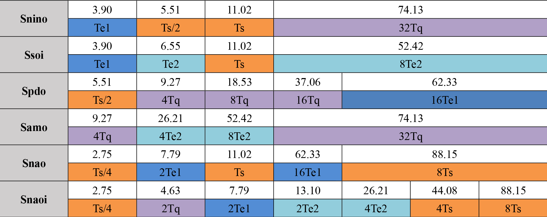
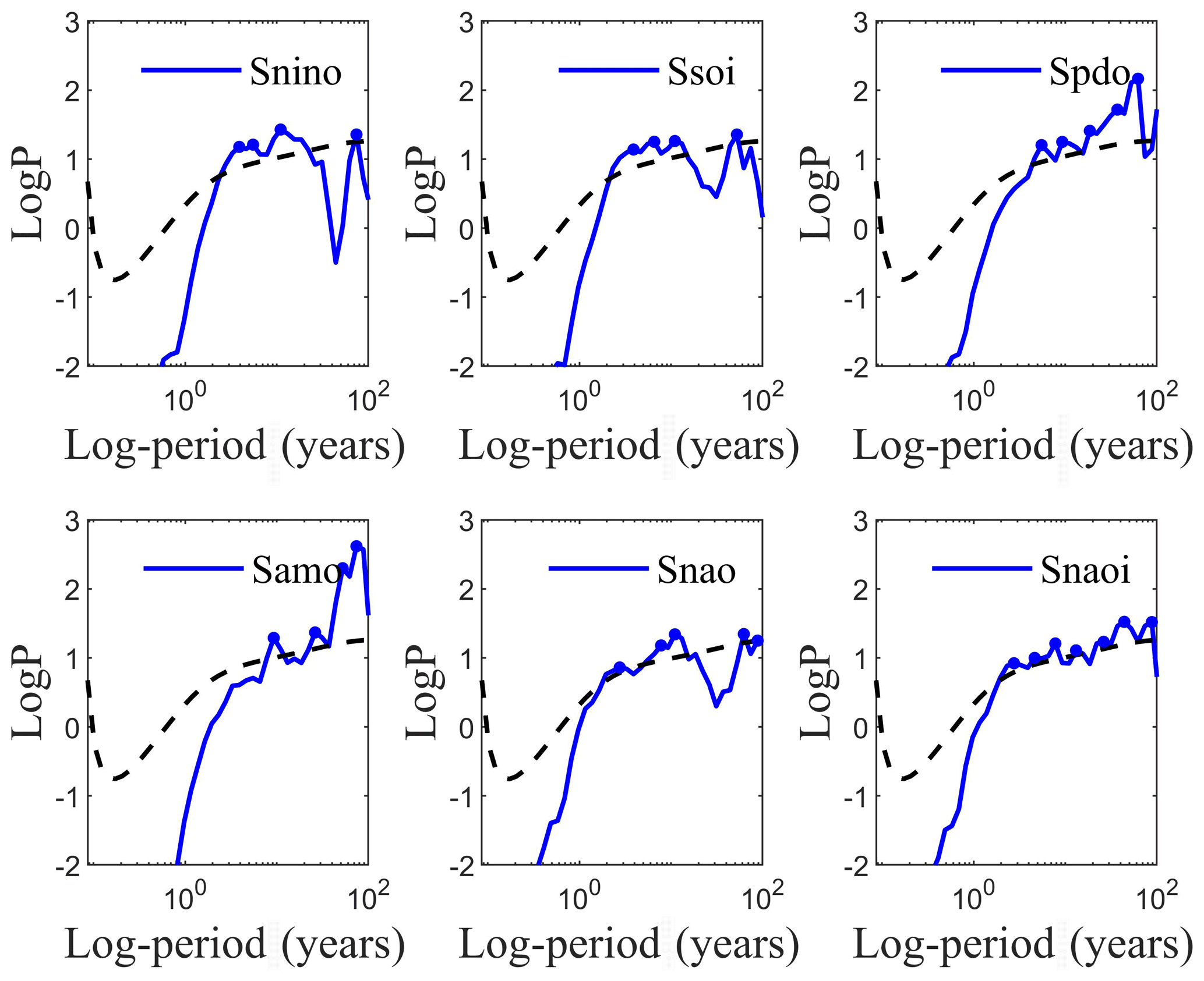
Figure 2The time-averaged power spectrum of SFA-extracted (m=11) slow feature signals for six climate indices; the significant points (blue dots) with peak power that pass the significance test at the 0.05 significance level (black dashed lines) are also indicated.
The peak period of 2.32 years (Tq, around 28 months) coincides with the cycle of the quasi-biennial oscillation (QBO) (Baldwin et al., 2001), which is the dominant pattern of variability in the tropical stratosphere and displays alternating downward-propagating easterly and westerly wind regimes. Although the QBO is a tropical stratospheric phenomenon, it affects not only the chemical constituents (e.g., water vapor, ozone, etc.) but also the stratospheric flow from pole to pole by changing the influences of extratropical waves. Specifically, through the effects on the polar vortex, the QBO modulates surface weather patterns indirectly (Baldwin et al., 2001). Previous studies suggested that the temperature gradient between the troposphere and stratosphere can modulate the Walker circulation and SST anomalies in the equatorial Pacific Ocean by altering the atmospheric stability and tropical deep convection (Huang et al., 2012).
We cautiously infer that the two periods (i.e., 3.90 years for Te1 and 6.55 years for Te2) are related to the intrinsic interannual variability of ENSO activities, and the period of 11.02 years (Ts) corresponds well to the Schwabe sunspot cycle (11 years). The results of harmonic analysis show that the peak periods of the SFA-derived signals from different climate indices can be expressed as integral multiples of base independent periods (i.e., Tq, Te1, Te2, and Ts), implying that these four independent periods associated with the QBO, ENSO, and solar activity can be regarded as three common driving factors for the variabilities of ENSO, PDO, AMO, and NAO.
Note that in Fig. 2, even though NAO and NAOI represent the same mode, the results are a bit different. The reason is that Fig. 2 is an illustration for an embedding dimension to 13. However, as Fig. 3 shows, when we vary the embedding dimension from 1 to 25, the peak periods of both NAO and NAOI show robust relations with ENSO, QBO, and solar activities. In a way, repeating for many embedding dimensions serves as a sensitivity analysis to see if the results are robust. Thus, even though this work does not directly assess the uncertainties on the peak values, our approach provides evidence of their robustness. In the Supplement, we present further results using an ideal model to confirm the effectiveness and robustness of the approach that combines SFA with wavelet analysis in extracting the driving factors of the dynamic system and their peak values. The results show that the significant peak periods of the SFA-derived signal reflect the true independent driving factors (Supplement Table S1; Figs. S1–S3).

Figure 3The significant peak periods of the SFA-extracted slow feature signals in six climate indices when setting different embedding dimensions from 1 to 25.
Given that the driving-force signal consists of several components, the selection of embedding dimension m may affect the phase-space reconstruction of time series (Konen and Koch, 2011; Yang et al., 2016). Considering that the peak periods of SFA-extracted driving-force signals may be sensitive to the embedding dimension m as set in SFA, we conduct an additional analysis by increasing m from 1 to 25 months (covering 2 years) to detect the significant peak periods of these driving-force signals. As Fig. 3 shows, all the significant peak periods can be represented as the integral multiples of Tq, Te1, Te2, and Ts, which confirms that the three abovementioned driving factors (QBO, the intrinsic variabilities of ENSO, and solar activities) are the common driving factors for the variabilities of ENSO, PDO, AMO, and NAO.
We further exploit the information involved in Fig. 3 and decompose it into tables. Table 2 shows the number of embedding dimensions by which a peak period is significant for each index. The two columns show the peak periods and their corresponding identifier (forcing). If the number is greater than 10, we highlight it in bold. Taking Snino for example, the entries in Table 2 show that 15∕25 embedding dimensions have a significant peak value at the period of 74.13 years (32Tq); 12∕25 embedding dimensions have a significant peak value at the period of 3.90 years (Te1); 16∕25 embedding dimensions have a significant peak value at the period of 5.51 years (0.5Ts); and 17∕25 embedding dimensions have a significant peak value at the period of 11.02 years (Ts).
Table 2The entries show, for each index, the number of embedding dimensions in which a peak period is significant. The left column lists the periods, and the right column shows the identifiers (forcings). If the number is greater than 10, it is highlighted in bold.
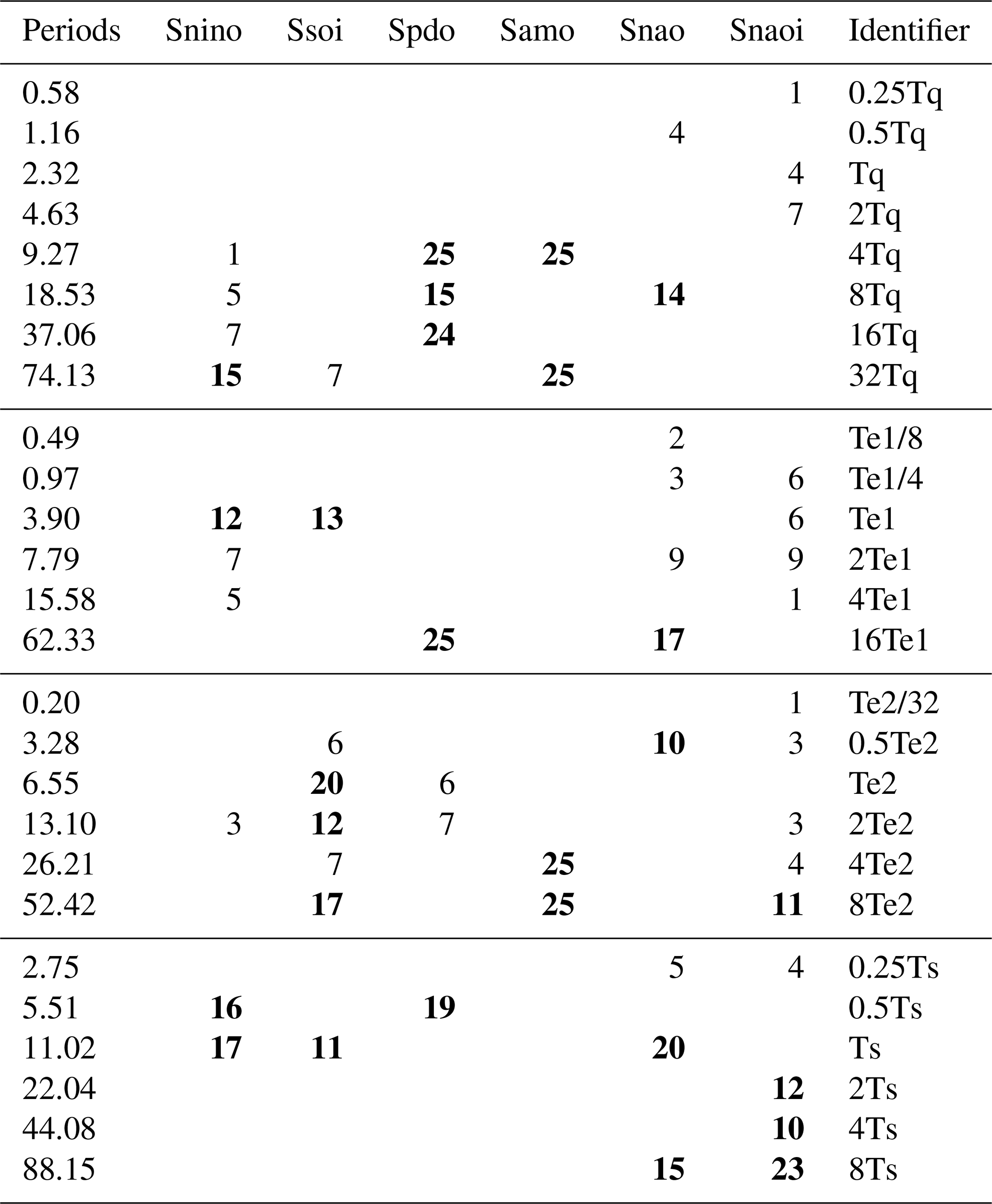
As shown in Table 2, each climate mode can be modulated by various driving factors that generate harmonic oscillations at different timescales. For instance, QBO presents four harmonic oscillations from interannual (9.27 years) to multidecadal (74.13 years) periods on NINO variability. The intrinsic variability of ENSO presents five harmonic oscillations from intra-seasonal (0.2 years) to multidecadal (52.42 years) timescales on the NAO variability. Similar results can be found for other climate indices.
In addition, we found that different climate indices involve the same driving harmonic oscillations. For instance, both PDO and AMO are modulated by the period of 9.27 years, which is a QBO-related harmonic oscillation. Both NINO and SOI are modulated by the period of 3.90 years, which we infer is linked to the intrinsic ENSO cycle. Both NINO and PDO are modulated by the interannual period of 5.51 years, which is a harmonic oscillation of solar activity.
The results displayed in Fig. 3 and Table 2 can be alternatively presented in Tables 3 and 4. In Table 3 the columns are the driving factors (Tq, Te1, Te2, and Ts) and the rows are the climate indices. The entries in the table show the harmonic(s) of driving-force factors affecting each index in more than 10 embedding dimensions. It shows that ENSO-Te1 presents the fewest harmonic peak periods and that solar, QBO, and ENSO-Te2 present an equally similar number of peak periods in shaping the variability of climate indices. Table 4 further shows the corresponding driving harmonic oscillations that modulate the variability of climate indices on various timescales (periods) for all embedding dimensions. The entries in bold correspond to the highlighted entries in Table 2.
Table 3The entries in the table show the harmonics of the basic driving forces (significant when affecting an index in more than 10 different embedding dimensions) for each climate mode index.
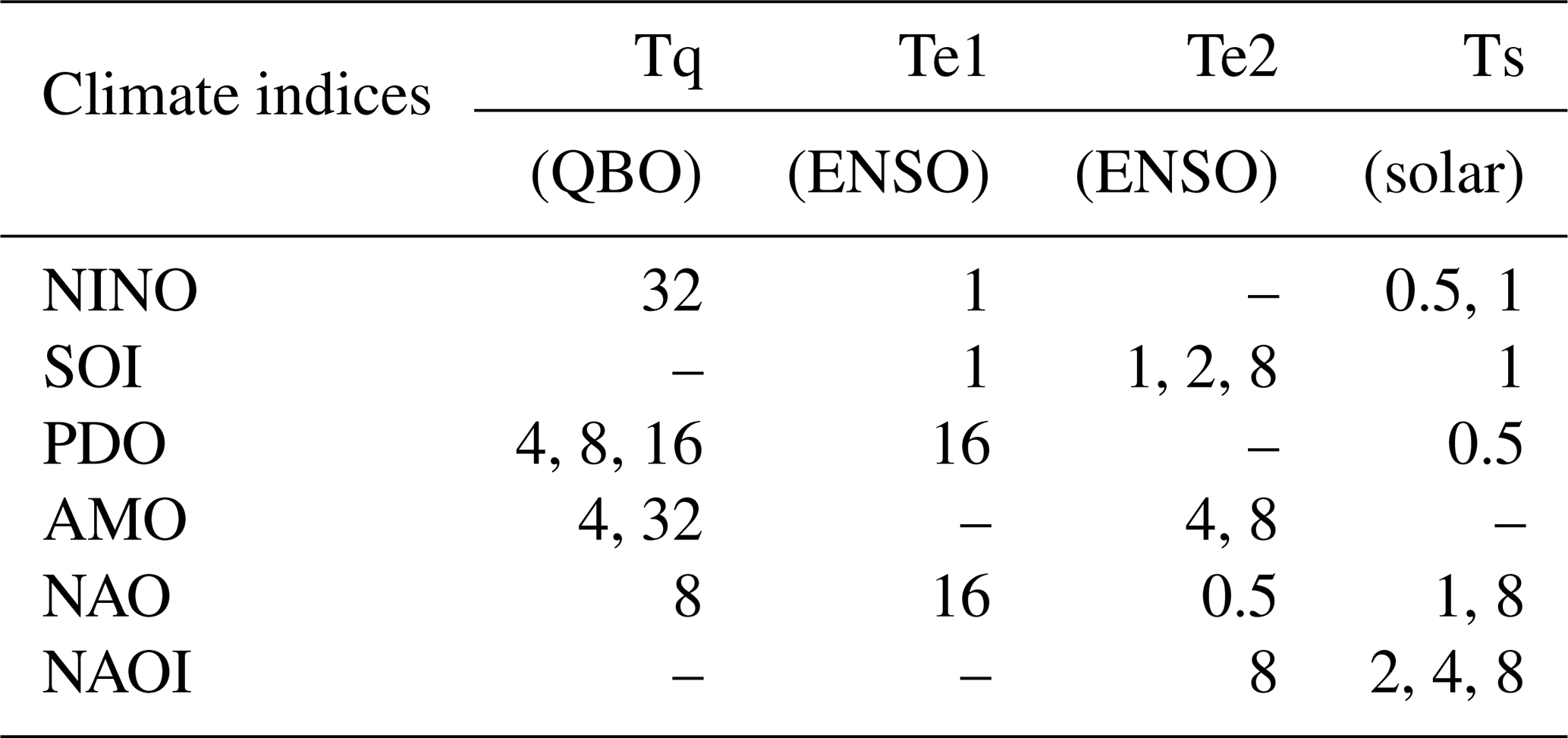
Table 4The basic driving forces and their harmonic oscillations that are associated with the variability of climate mode indices at various timescales (periods) for all embedding dimensions. The entries in bold correspond to the highlighted numbers in Table 3.
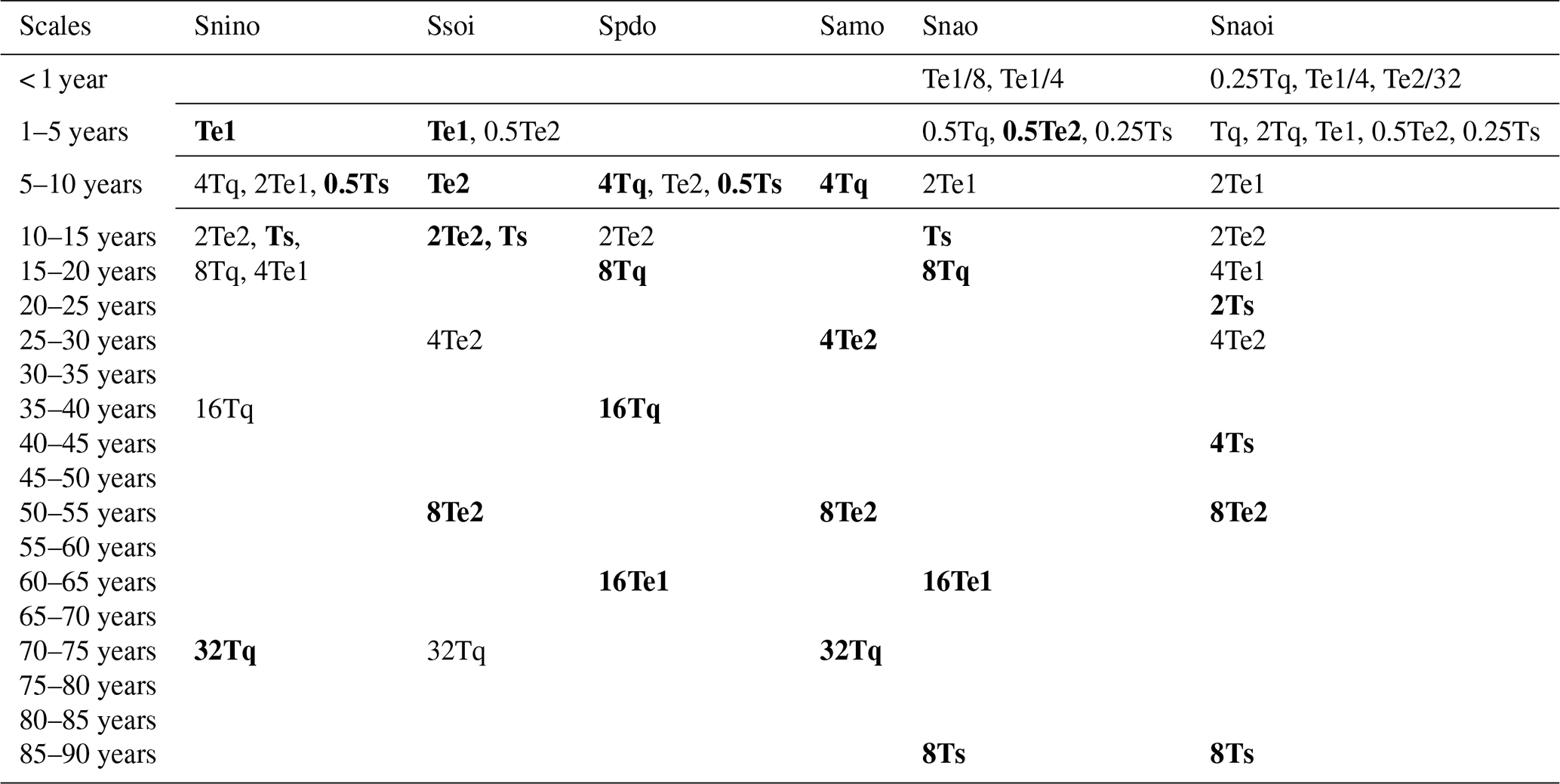
As shown in Table 4 the driving harmonic oscillations among different climate indices are diverse and complicated in periods less than 20 years in most conditions. Taking NAOI as an example, there are up to five driving harmonic oscillations on similar timescales (1–5 years). Nevertheless, the driving harmonic oscillations in the multidecadal period of 50–55 years are only related to ENSO-Te2, and the ones in the period of 60–65 years are only associated with ENSO-Te1. For the driving harmonic oscillations in the period of 70–75 years, the QBO is identified as the primary influencing factor. The driving harmonic oscillations in the period of 80–85 years appear to be linked to Ts.
Based on the results obtained by combining SFA with wavelet analysis, we find that all the detected peak periods can be represented as the integral multiples of the base peak periods associated with QBO, intrinsic variabilities of ENSO, and solar activities. Considering that the time series of AMO used in this study is unsmoothed, we repeat the analysis by using the smoothed AMO index (with a 121-month smoother). The peak periods detected in the smoothed time series are exactly the same as the ones based on the unsmoothed index (figure not shown). This means that the preprocessing of the AMO index has little effect on the application of SFA and its related results.
In this study, we identify four independent base peak periods: Tq (2.32 years), Te1 (3.90 years), Te2 (6.55 years), and Ts (11.02 years). We cautiously infer that these base peak periods are essentially associated with the QBO cycle, two intrinsic ENSO cycles, and the solar cycle, respectively. Other detected significant peak periods can be represented by the integral multiples of these four base periods. This implies that the QBO, ENSO, and solar activities could be three key periodic driving factors in global climate variability. These results provide possible clues for the intricate relationships between driving forces and their harmonics in the variability of major climate modes as well as the coupling paths among them. The finding of the interconnections of major climate modes indicates that using statistical models to predict decadal to multidecadal climate variability could be promising in the future. It should be noted that uncertainties still exist in the multidecadal variability of ENSO and QBO. The relatively long peak periods (e.g., 52.42, 62.33, 74.13, and 88.15 years) detected by SFA may result from the effect of continuous wavelet transform.
Recent studies on complex climate networks have provided new insights into how the collective behavior of major climate modes affects global temperature variations (Tsonis et al., 2007; Tsonis, 2018). By considering a network of major climate modes (more or less the same set as here) and the theory of synchronized chaos, these previous studies found that the network may synchronize temporally. During synchronization, the increased coupling strength among the climate modes may lead to the destruction of the synchronized state, which leads to changes in the trends of global temperature and the amplitudes of ENSO variability on decadal to multidecadal timescales. These studies proposed a dynamical mechanism and its related physical causes for the observed climate shifts. The idea that the interaction between major climate modes plays a significant role in climate variability has found many applications in the last decade or so.
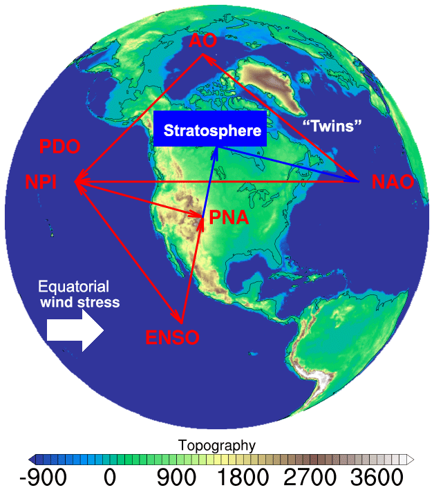
Figure 4The 3-D super-loop NAO → PDO → ENSO → PNA → stratosphere → NAO, which may capture the essence of low-frequency variability in the Northern Hemisphere.
Solid dynamical arguments and past work offer a concrete picture of how the physics may play out (Wang et al., 2009). NAO, with its huge mass rearrangement in the North Atlantic, affects the strength of the westerly flow across midlatitudes. At the same time, through its “twin”, the Arctic Oscillation (AO), it affects sea level pressure patterns in the northern Pacific. This process is part of the so-called intrinsic midlatitude Northern Hemisphere variability. Then, this intrinsic variability, through the seasonal “footprinting” mechanism, couples with equatorial wind stress anomalies, thereby acting as a stochastic forcing of ENSO. Subsequently, ENSO, with its effects on PNA, can influence the lower stratosphere through the vertical propagation of Rossby waves, and in turn the stratosphere influences NAO through the downward progression of Rossby waves. These results, coupled with our results, suggest the following 3-D super-loop NAO → PDO → ENSO → PNA → stratosphere → NAO, which may capture the essence of low-frequency variability in the Northern Hemisphere (Fig. 4).
While still more work is needed on the physical and dynamical links among major climate modes and their interactions, our results here provide additional possible players in the above picture. Solar activity can be linked to the stratosphere (see Roy, 2018, for example). Solar activity affects the QBO and thus the stratosphere, which together with ENSO are implicated in this 3-D loop. Our results provide further new insights into those dynamical mechanisms and how the complex interactions among the base driving factors and their harmonics may cause peak periods in climate modes and thus affect climate variability.
All data needed to evaluate the conclusions in the paper are presented in the paper. Additional data and codes related to this paper may be requested from the corresponding author.
The supplement related to this article is available online at: https://doi.org/10.5194/esd-11-525-2020-supplement.
XP and GW designed this study. All of the authors contributed to the preparation and writing of the paper.
The authors declare that they have no conflict of interest.
This research was supported by the National Key R&D Program of China (2017YFC1501804) and the National Natural Science Foundation of China (91737102 and 41575058).
This research has been supported by the National Key R&D Program of China (grant no. 2017YFC1501804) and the National Natural Science Foundation of China (grant nos. 91737102 and 41575058).
This paper was edited by Ben Kravitz and reviewed by two anonymous referees.
Baldwin, M. P., Gray, L. J., Dunkerton, T. J., Hamilton, K., Haynes, P. H., Randel, W. J., Holton J. R., Alexander, M. J., Hirota, I., Horinouchi, T., Jones, D. B. A., Kinnersley, J. S., Marquardt, C., Sato, K., and Takahashi M..: The quasi-biennial oscillation, Rev. Geophys., 39, 179–229, https://doi.org/10.1029/1999rg000073, 2001.
Bjerknes, J.: Atmospheric teleconnections from the equatorial pacific, Mon. Weather Rev., 97, 163–172, https://doi.org/10.1175/1520-0493(1969)0972.3.CO;2, 1969.
Blaschke, T., Berkes, P., and Wiskott, L.: What is the relation between slow feature analysis and independent component analysis?, Neural Comput., 18, 2495–2508, https://doi.org/10.1162/neco.2006.18.10.2495, 2006.
Bradley, R. S., Diaz, H. F., Kiladis, G. N., and Eischeid, J. K.: ENSO signal in continental temperature and precipitation records, Nature, 327, 497–501, https://doi.org/10.1038/327497a0, 1987.
Capotondi, A., Wittenberg, A. T., Newman, M., Di Lorenzo, E., Yu, J. Y., Braconnot, P., Cole, J., Dewitte, B., Giese, B., Guilyardi, E., Jin, F. F., Karnauskas, K., Kirtman, B., Lee, T., Schneider, N., Xue, Y., and Yeh, S. W.: Understanding ENSO diversity, B. Am. Meteorol. Soc., 96, 921–938, https://doi.org/10.1175/BAMS-D-13-00117.1, 2015.
Dai, A. G.: Recent climatology, variability, and trends in global surface humidity, J. Climate, 19, 3589–3606, https://doi.org/10.1175/JCLI3816.1, 2006.
Delworth, T. L. and Mann, M. E.: Observed and simulated multidecadal variability in the Northern Hemisphere, Clim. Dynam., 16, 661–676, https://doi.org/10.1007/s003820000075, 2000.
Delworth, T. L., Zeng, F. R., Zhang, L. P., Zhang, R., Vecchi, G. A., and Yang, X. S.: The central role of ocean dynamics in connecting the North Atlantic Oscillation to the extratropical component of the Atlantic Multidecadal Oscillation, J. Climate, 30, 3789–3805, https://doi.org/10.1175/JCLI-D-16-0358.1, 2017.
Deser, C., Alexander, M. A., Xie, S. P., and Phillips, A. S.: Sea surface temperature variability: patterns and mechanisms, Ann. Rev. Mar. Sci., 2, 115–143, https://doi.org/10.1146/annurev-marine-120408-151453, 2010.
Enfield, D. B., Mestas-Nuñez, A. M., and Trimble, P. J.: The Atlantic multidecadal oscillation and its relation to rainfall and river flows in the continental U.S., Geophys. Res. Lett., 28, 2077–2080, https://doi.org/10.1029/2000gl012745, 2001.
Escalante-B., A. N. and Wiskott, L.: Slow feature analysis: perspectives for technical applications of a versatile learning algorithm, KI-Künstliche Intelligenz, 26, 341–348, https://doi.org/10.1007/s13218-012-0190-7, 2012.
Franzius, M., Wilbert, N., and Wiskott, L.: Invariant object recognition and pose estimation with slow feature analysis, Neural Comput., 23, 2289–2323, https://doi.org/10.1162/NECO_a_00171, 2011.
Garuba, O. A., Lu, J., Singh, H. A., Liu, F. K., and Rasch, P.: On the relative roles of the atmosphere and ocean in the Atlantic multidecadal variability, Geophys. Res. Lett., 45, 9186–9196, https://doi.org/10.1029/2018GL078882, 2018.
Huang, B. H., Hu, Z. Z., Kinter, J. L., Wu, Z. H., and Kumar, A.: Connection of stratospheric QBO with global atmospheric general circulation and tropical SST. part I: methodology and composite life cycle, Clim. Dynam., 38, 1–23, https://doi.org/10.1007/s00382-011-1250-7, 2012.
Hurrell, J. W.: Decadal trends in the North Atlantic Oscillation: regional temperatures and precipitation, Science, 269, 676–679, https://doi.org/10.1126/science.269.5224.676, 1995.
Jajcay, N., Hlinka, J., Kravtsov, S., Tsonis, A. A., and Paluš, M.: Time-scales of the European surface air temperature variability: The role of the 7–8 year cycle, Geophys. Res. Lett., 43, 902–909, https://doi.org/10.1002/2015GL067325, 2016.
Jones, P. D., Jonsson, T., and Wheeler, D.: Extension to the North Atlantic oscillation using early instrumental pressure observations from Gibraltar and south-west Iceland, Int. J. Climatol., 17, 1433–1450, https://doi.org/10.1002/(sici)1097-0088(19971115)17:13<1433::aid-joc203>3.0.co;2, 1997.
Kenyon, J. and Hegerl, G. C.: Influence of modes of climate variability on global temperature extremes, J. Climate, 21, 3872–3889, https://doi.org/10.1175/2008JCLI2125.1, 2008.
Kirov, B. and Georgieva, K.: Long-term variations and interrelations of ENSO, NAO and solar activity, Phys. Chem. Earth, 27, 441–448, https://doi.org/10.1016/S1474-7065(02)00024-4, 2002.
Knight, J. R., Folland, C. K., and Scaife, A. A.: Climate impacts of the Atlantic Multidecadal Oscillation, Geophys. Res. Lett., 33, L17706, https://doi.org/10.1029/2006GL026242, 2006.
Konen, W. and Koch, P.: The slowness principle: SFA can detect different slow components in non-stationary time series, Int. J. Innov. Comp. Appl., 3, 3–10, https://doi.org/10.1504/IJICA.2011.037946, 2011.
Li, J. P. and Wang, J. X. L.: A new North Atlantic Oscillation index and its variability, Adv. Atmos. Sci., 20, 661–676, https://doi.org/10.1007/BF02915394, 2003.
Li, J. P., Sun, C., and Jin, F. F.: NAO implicated as a predictor of Northern Hemisphere mean temperature multidecadal variability, Geophys. Res. Lett., 40, 5497–5502, https://doi.org/10.1002/2013GL057877, 2013.
Liu, Z. Y. and Alexander, M.: Atmospheric bridge, oceanic tunnel, and global climatic teleconnections, Rev. Geophys., 45, RG2005, https://doi.org/10.1029/2005RG000172, 2007.
Mantua, N. J. and Hare, S. R.: The Pacific Decadal Oscillation, J. Oceanogr., 58, 35–44, https://doi.org/10.1023/A:1015820616384, 2002.
Mantua, N. J., Hare, S. R., Zhang, Y., Wallace, J. M., and Francis, R. C.: A Pacific interdecadal climate oscillation with impacts on salmon production, B. Am. Meteorol. Soc., 78, 1069–1079, https://doi.org/10.1175/1520-0477(1997)078<1069:APICOW>2.0.CO;2, 1997.
McCabe, G. J., Palecki, M. A., and Betancourt, J. L.: Pacific and Atlantic Ocean influences on multidecadal drought frequency in the United States, P. Natl. Acad. Sci. USA, 101, 4136–4141, https://doi.org/10.1073/pnas.0306738101, 2004.
Newman, M., Compo, G. P., and Alexander, M. A.: ENSO-forced variability of the Pacific Decadal Oscillation, J. Climate, 16, 3853–3857, https://doi.org/10.1175/1520-0442(2003)016<3853:EVOTPD>2.0.CO;2, 2003.
Newman, M., Alexander, M. A., Ault, T. R., Cobb, K. M., Deser, C., Di Lorenzo, E., Mantua, N. J., Miller, A. J., Minobe, S., Nakamura, H., Schneider, N., Vimont, D. J., Phillips, A. S., Scott, J. D., and Smith, C. A.: The pacific decadal oscillation, revisited, J. Climate, 29, 4399–4427, https://doi.org/10.1175/JCLI-D-15-0508.1, 2016.
Pan, X. N., Wang, G. L., and Yang, P. C.: Extracting the driving force signal from hierarchy system based on slow feature analysis, Acta Phys. Sin., 66, 080501, https://doi.org/10.7498/aps.66.080501, 2017.
Rayner, N. A., Parker, D. E., Horton, E. B., Folland, C. K., Alexander, L. V., Rowell, D. P., Kent, E. C., and Kaplan, A.: Global analyses of sea surface temperature, sea ice, and night marine air temperature since the late nineteenth century, J. Geophys. Res., 108, 4407, https://doi.org/10.1029/2002jd002670, 2003.
Ropelewski, C. F. and Jones, P. D.: An extension of the Tahiti–Darwin southern oscillation index, Mon. Weather Rev., 115, 2161–2165, https://doi.org/10.1175/1520-0493(1987)1152.0.CO;2, 1987.
Rossi, A., Massei, N., and Laignel, B.: A synthesis of the time-scale variability of commonly used climate indices using continuous wavelet transform, Global Planet. Change, 78, 1–13, https://doi.org/10.1016/j.gloplacha.2011.04.008, 2011.
Roy, I. (Ed.): Climate variability and sunspot activity: Analysis of solar influence on climate, Springer, ISBN 978-3-319-77106-9, 2018.
Schlesinger, M. E. and Ramankutty, N.: An oscillation in the global climate system of period 65–70 years, Nature, 367, 723–726, https://doi.org/10.1038/372508a0, 1994.
Steinman, B. A., Mann, M. E., and Miller, S. K.: Atlantic and Pacific multidecadal oscillations and Northern Hemisphere temperatures, Science, 347, 988–991, https://doi.org/10.1126/science.1257856, 2015.
Sun, C., Li, J. P., and Jin, F. F.: A delayed oscillator model for the quasi-periodic multidecadal variability of the NAO, Clim. Dynam., 45, 2083–2099, https://doi.org/10.1007/s00382-014-2459-z, 2015.
Torrence, C. and Compo, G. P.: A practical guide to wavelet analysis, B. Am. Meteorol. Soc., 79, 61–78, https://doi.org/10.1175/1520-0477(1998)079<0061:APGTWA_2.0.CO;2, 1998.
Trenberth, K. E., Branstator, G. W., Karoly, D., Kumar, A., Lau, N. C., and Ropelewski, C.: Progress during TOGA in understanding and modeling global teleconnections associated with tropical sea surface temperatures, J. Geophys. Res.-Atmos., 103, 14291–14324, https://doi.org/10.1029/97jc01444, 1998.
Tsonis, A. A.: Insights in climate dynamics from climate networks, Adv. Nonlinear Geosci., 631–649, https://doi.org/10.1007/978-3-319-58895-7_29, 2018.
Tsonis, A. A., Swanson, K., and Kravtsov, S.: A new dynamical mechanism for major climate shifts, Geophys. Res. Lett., 34, L13705, https://doi.org/10.1029/2007GL030288, 2007.
Tsonis, A. A., Swanson, K. L., and Wang, G. L.: On the role of atmospheric teleconnections in climate, J. Climate, 21, 2990–3001, https://doi.org/10.1175/2007JCLI1907.1, 2008.
Velasco, V. M. and Mendoza, B.: Assessing the relationship between solar activity and some large scale climatic phenomena, Adv. Space Res., 42, 866–878, https://doi.org/10.1016/j.asr.2007.05.050, 2008.
Verdes, P. F., Granitto, P. M., Navone, H. D., and Ceccatto, H. A.: Nonstationary time-series analysis: Accurate reconstruction of driving forces, Phys. Rev. Lett., 87, 124101, https://doi.org/10.1103/PhysRevLett.87.124101, 2001.
Wallace, J. M. and Gutzler, D. S.: Teleconnections in the geopotential height field during the northern hemisphere winter, Mon. Weather Rev., 109, 784–812, https://doi.org/10.1175/1520-0493(1981)109<0784:TITGHF>2.0.CO;2, 1981.
Wang, G. L., Swanson, K. L., and Tsonis, A. A.: The pacemaker of major climate shifts, Geophys. Res. Lett., 36, L07708, https://doi.org/10.1029/2008GL036874, 2009.
Wang, G. L., Yang, P. C., and Zhou, X. J.: Extracting the driving force from ozone data using slow feature analysis, Theor. Appl. Climatol., 124, 985–989, https://doi.org/10.1007/s00704-015-1475-1, 2016.
Wang, G. L., Yang, P. C., and Zhou, X. J.: Identification of the driving forces of climate change using the longest instrumental temperature record, Sci. Rep.-UK, 7, 46091, https://doi.org/10.1038/srep46091, 2017.
Wiskott, L. and Sejnowski, T. J.: Slow feature analysis: Unsupervised learning of invariances, Neural Comput., 14, 715–770, https://doi.org/10.1162/089976602317318938, 2002.
Wu, R. G., Hu, Z. Z., and Kirtman, B. P.: Evolution of ENSO-related rainfall anomalies in East China, J. Climate, 16, 3742–3758, https://doi.org/10.1175/1520-0442(2003)016<3742:eoerai>2.0.co;2, 2003.
Xie, T. J., Li, J. P., Sun, C., Ding, R. Q., Wang, K. C., Zhao, C. F., and Feng J.: NAO implicated as a predictor of the surface air temperature multidecadal variability over East Asia, Clim. Dynam., 53, 895–905, https://doi.org/10.1007/s00382-019-04624-4, 2019.
Yang, P. C., Bian, J. C., Wang, G. L., and Zhou, X. J.: Hierarchy and non-stationarity in climate systems: Exploring the prediction of complex systems, Chinese Sci. Bull., 48, 2148–2154, https://doi.org/10.1360/03wd0175, 2003.
Yang, P. C., Wang, G. L., Zhang, F., and Zhou, X. J.: Causality of global warming seen from observations: a scale analysis of driving force of the surface air temperature time series in the Northern Hemisphere, Clim. Dynam., 46, 3197–3204, https://doi.org/10.1007/s00382-015-2761-4, 2016.
Zhang, F., Lei, Y. D., Yu, Q. R., Fraedrich, K., and Iwabuchi, H.: Causality of the drought in the southwestern United States based on observations, J. Climate, 30, 4891–4896, https://doi.org/10.1175/JCLI-D-16-0601.1, 2017.
Zhang, R.: Anticorrelated multidecadal variations between surface and subsurface tropical North Atlantic, Geophys, Res. Lett., 34, L12713, https://doi.org/10.1029/2007GL030225, 2007.
Zhang, R.: On the persistence and coherence of subpolar sea surface temperature and salinity anomalies associated with the Atlantic multidecadal variability, Geophys. Res. Lett., 44, 7865–7875, https://doi.org/10.1002/2017GL074342, 2017.