the Creative Commons Attribution 4.0 License.
the Creative Commons Attribution 4.0 License.
 | 15 Aug 2018
A mathematical approach to understanding emergent constraints
Henk A. Dijkstra
One of the approaches to constrain uncertainty in climate models is the identification of emergent constraints. These are physically explainable empirical relationships between a particular simulated characteristic of the current climate and future climate change from an ensemble of climate models, which can be exploited using current observations. In this paper, we develop a theory to understand the appearance of such emergent constraints. Based on this theory, we also propose a classification for emergent constraints, and applications are shown for several idealized climate models.
- Article
(2086 KB) - Full-text XML
- BibTeX
- EndNote


Improving the accuracy of climate projections is one of the most important challenges in climate modelling. The uncertainty can be reduced by the development of more and more sophisticated global climate models, capturing more processes and scales. However, the societal importance of climate projections calls for a faster pace of improvement and alternative approaches that aim to better determine the accuracy of existing models. One of the proposed methods to accomplish this has been the use of so-called emergent constraints, where current observations are used to constrain future projections (Collins et al., 2012).
In multi-model ensembles of complex climate models, an apparent linear relation can be found between short-term and long-term changing variables. More credibility is attached to models that match the observed variability or trend well over the recent period. In this way, current observations provide a constraint to long-term trends. The observed variable is called the predictor, while the variable that is to be constrained is called the predictand (Klein and Hall, 2015). In recent years, emergent constraints have been found for Arctic warming, snow-albedo feedback, tropical carbon, the global precipitation among other variables (Allen and Ingram, 2002; Bracegirdle and Stephenson, 2013; Hall and Qu, 2006; Wenzel et al., 2014) and more recently, climate sensitivity (Cox et al., 2018).
A prominent example is the emergent constraint found in Hall and Qu (2006) where an emergent relationship was found between the strength of the snow-albedo feedback (SAF) on a seasonal timescale and the SAF under global warming in a Coupled Model Intercomparison Project phase 3 (CMIP3) ensemble. They also elucidated the key physical process behind the emergent constraint. Models where the maximum albedo of snow is highest have the largest SAF on both timescales because the contrast between snow-covered and snow-free areas is high (Qu and Hall, 2007).
However, a more general dynamical picture on how emergent constraints occur in multi-model ensembles or even in a parameter ensemble of a single model is still lacking. Under which circumstances are these constraints expected to arise? Some emergent constraints may be spurious and could arise because of shared errors in a particular multi-model ensemble (Bracegirdle and Stephenson, 2013). A mathematical framework is desired to identify spurious constraints and to give an indication as to where new emergent constraints might arise.
Here, we investigate how and under what conditions emergent constraints appear and what can be learned about the physics of the climate system. We will use linear response theory (LRT) to address the problem of forcing-response relations on different timescales (Risken, 1996). Ruelle demonstrated that LRT can be extended to study the response of non-equilibrium systems to external forcing. As with the fluctuation–dissipation theorem, Ruelle's LRT uses the statistical properties of the unforced (equilibrium) state only, but it does not assume (quasi)-equilibrium. Recently, LRT has been proposed as a rigorous framework for computing the response of the climate system and its applicability has been tested on the Lorenz-96 model and on the idealized global climate model PlaSim (Lucarini and Sarno, 2011; Ragone et al., 2016).
The paper is organized as follows. To obtain an understanding of emergent constraints, we start by formulating a mathematical framework in terms of susceptibilities by making use of LRT (Sect. 2). This results in explicit expressions for the appearance of emergent constraints in terms of susceptibility functions. In Sect. 3, a classification scheme for emergent constraints is proposed. Then, in Sect. 4, applications are presented for conceptual climate models, such as Ornstein–Uhlenbeck processes in one and two dimensions, an energy balance model and the PlaSim model. The results are summarized and discussed in Sect. 5.
In this section, explicit expressions are given for response functions of the state of a dynamical system which depends on a single parameter and which is subjected to a non-stationary forcing. Such response functions are used in the following section to classify the different emergent constraints. Rigorous results for linear response properties of large class of general stochastic systems was obtained by Hairer and Majda (2010) (linear response theory for non-equilibrium systems was developed by Ruelle, 1998, 2009).
We illustrate the approach using the general one-dimensional forced stochastic differential equation (SDE):
Here, V(x) is a smooth confining potential, meaning that a equilibrium solution exists for the unforced system (Pavliotis, 2014), and F(t) is a prescribed forcing. Furthermore, σ is the noise amplitude and the associated Wiener process is indicated by Wt. Usually, the potential depends on a parameter.
The probability density function of the unforced (F(t)=0) system, say , satisfies the Fokker–Planck equation:
which defines the Fokker–Planck operator ℒ*. The equilibrium distribution of the unforced system, here indicated by , is given by
Linear response theory (Ragone et al., 2016) provides an expression for the change in the expectation value of the change in an observable O (e.g. the temperature, ice extent or the standard deviation of either), say ΔO(t) when the system is forced, compared to the unforced case, i.e.
where again the subscript “e” indicates the equilibrium of the unforced system. It follows that
where RO(t) is the response function, which is extended to be zero for t<0 to ensure causality with a Heaviside function ℋ(t). When Eq. (5) is Fourier transformed, we find, using the convolution theorem,
where the Fourier transform χ(ω) of the response function RO(t) is the susceptibility. If we take a cosine forcing, i.e. F(t)=F0cosω0t, then , so once we know χ(ω), we can determine the response ΔO(t).
In the Appendix, it is shown that when we take the identity operator O=x as the observable, thus taking the mean value of this variable, the response function and its corresponding susceptibility can be written as
where λl indicates the eigenvalues of the so-called generator ℒ,
and the βl represents projection coefficients that indicate how strongly the system responds to the forcing; see the Appendix for a more detailed description.
The amplitude A of the response to a periodic forcing F(t)=F0cosω0t is determined by the absolute value of the susceptibility:
When the predictor is a response to a uniform frequency forcing, it can be expressed as in Eq. (9). The predictand will generally also have this form, as a forcing with a long timescale can be approximated by a low-frequency forcing. The previous analysis can be generalized to more dimensions. In two dimensions, for example, with a state vector , the SDE becomes
where the term denotes a forcing in the direction of the first variable and I2 the identity matrix. As shown in Pavliotis (2014), the derivation of the response function follows the one-dimensional case closely, resulting in
where gl and hl are again projection coefficients; gl and hl contain a term describing strength of the response in Y1 and Y2, respectively. The derivation of the exact terms is given in the Appendix. Calculating the response is analogous to the one-dimensional case, so that the Fourier transforms of the response functions are given by
Note that, generalizing to uncoupled multidimensional systems, the eigenfunctions are found to be the tensor products of the eigenfunctions in the one-dimensional case, while the corresponding eigenvalues are the sum of the eigenvalues in the one-dimensional case.
Although a wide set of different emergent constraints has been found, no attempts have been made to classify them so far using dynamical criteria. Here, a classification is proposed based on the time characteristics of the predictor and on the relationship between the predictor and the predictand. Using this classification, assessment of their applicability becomes easier. Furthermore, a classification is a prerequisite for a dynamical description of emergent constraints.
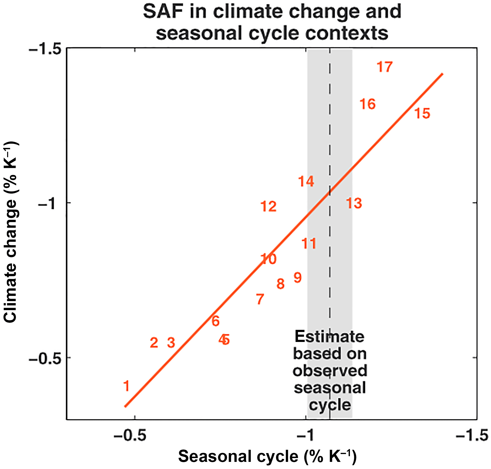
Figure 1The emergent constraint on snow-albedo feedback (from Hall and Qu, 2006, αs given in units of percent). This is an example of a direct emergent constraint (it links the SAF in both past and future time) and a dynamical emergent constraint (it uses a response to a seasonal forcing as its predictor).
Firstly, an emergent constraint can be either direct or indirect. In the direct case, the predictor and predictand are the same observable, while in the indirect case they are not. In the latter case, the predictor variable and predictand variable have to be closely linked, for instance, via a physical process. We make a further distinction between static and dynamic emergent constraints. In a dynamic emergent constraint, a response to a known, or sometimes even unknown, forcing in the (present-day) predictor is linked to the response of the (future) predictand under the same (or a similar) forcing. For example, the forcing can be the annual cycle of solar radiation but can also be caused by ENSO or historical climate change. In a static emergent constraint, a relationship between the time-independent quantity of the unforced system in the present-day (predictor) is linked to the response in a quantity under climate change.
Knutti et al. (2006)Hall and Qu (2006); Qu and Hall (2014)Boe et al. (2009)Clement et al. (2009)Trenberth and Fasullo (2010)Fasullo and Trenberth (2012)Bracegirdle and Stephenson (2013)Gordon and Klein (2014)Qu et al. (2014)Sherwood et al. (2014)Su et al. (2014)Wenzel et al. (2014)Tian (2015)Kwiatkowski et al. (2017)Cox et al. (2018)Table 1Application of our classification of emergent constraints to a selection of examples found in literature. DD is a direct dynamical constraint, DS is a direct static constraint, and IS is an indirect static constraint, while ID denotes indirect dynamical emergent constraints. Abbreviations are as follows: RH: relative humidity, ITCZ: Intertropical Convergence Zone, TOA: top of atmosphere, SH: Southern Hemisphere, ECS: equilibrium climate sensitivity, LLC: low-level cloud, SAF: snow-albedo feedback, SAT: surface air temperature; GMST: global mean surface temperature. The emergent constraint found by Trenberth and Fasullo (2010) seems to be spurious: no physical mechanism was proposed and it did not appear in different ensembles, such as CMIP5 (Grise et al., 2015).
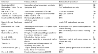
As an illustration, we apply our classification to examples of emergent constraints found in the literature in Table 1. Although this is not a complete overview, examples are found of the four types of emergent constraints. There are many examples of direct dynamical constraints, such as the one involving the snow-albedo feedback shown in Fig. 1 (Hall and Qu, 2006). Dynamic direct emergent constraints are the most intuitive. As long as the variations in the predictor are of a sufficient amplitude compared to those of the predictand, a correlation between the predictor and predictand automatically points towards a common physical basis, for example, a common dynamical response to an external forcing. The direct static emergent constraint found by Bracegirdle and Stephenson (2013) makes use of spatial patterns. All of the indirect constraints involve equilibrium climate sensitivity as the predictand. Often the mean of some variable with some known bias in the model ensemble is linked to ECS. For instance, in Tian (2015), the asymmetry bias in the Intertropical Convergence Zone (ITCZ) is linked to climate sensitivity. An example of a dynamical indirect emergent constraint is provided by Cox et al. (2018), who relate a function of autocorrelation of global surface temperature to ECS. In this case, the short-time forcing is assumed to be caused by internal variability.
Based on the response function theory in Sect. 2, we further elaborate on the classification and also discuss conditions for each type of constraint for a dynamical system with varying parameters (which defines the ensemble of models).
For a direct dynamical emergent constraint, in the standard case of a linear relationship, the relation has the following form: Predictand = Cst× Predictor, where Cst is a constant that is independent of the parameter used to generate the ensemble of models. Rewriting this, the ratio of the responses to forcing of frequencies ω1 and ω2 should be constant over the (parameter) ensemble members ei. For the simple case of two forcings that only differ in frequency, we find the condition from the ratio of the susceptibilities SR as
One variable (B) can act as forcing to a second variable (O), while being itself forced externally (F). The predictor and predictand are then given by the quotient of the response functions of O and B. A further complication is that often the forcing patterns are not exactly the same for the short (F2) and long (F1) periodic forcing. In this case, (Eq. 15) has to be adjusted to
This is further discussed in the example of the idealized energy balance model.
Physically, we expect that the same mechanism is responsible for the response at a short and long timescale to obtain this type of emergent constraint. The system should have response times smaller than the timescale of the forcing or equivalently: the generator should have eigenvalues λ larger than the frequency of the forcing. Naturally, the response times of the dominant processes are expected to be at least smaller than the timescale of the slow forcing .
Mathematically, the ratio in Eq. (15) becomes 1 in the case that all eigenvalues λl are much larger than the forcing frequencies. Interestingly, the linear relation breaks down in the case that the fast forcing has the same order of magnitude as the eigenvalues of the dominant terms in the susceptibility. Under the assumption of a single dominant term in the susceptibility and a slow forcing with frequency ω2→0, the first correction term to the slope-one linear relation between predictand y and predictor x, is cubic in x.
In the case of indirect dynamical emergent constraints, a relationship between a predictor Y1 and a predictand Y2 is found. Assuming the predictor Y1 is again a response to some forcing, we can repeat the analysis above for direct constraints for a system of two dimensions, where a forcing is added in one direction. Mutatis mutandis, a condition very similar to Eq. (15) is found, as
where gl and hl are defined as in Eq. (12). For an emerging constraint to exist, the projection terms of the different observables should thus change in a similar fashion under the change in parameter.
Static direct constraints link the mean of an observable (predictor) to a change in the system under a specific forcing (predictand). Note that the susceptibility only contains information about the response to such forcing. Even in the limit of ω→0, it denotes the linear response of the system, without any information on the mean state (Lucarini and Sarno, 2011). So, to derive the condition for a linear relationship, the mean and the susceptibility at frequency ω1 are used.
For static emergent constraints, the linear relationship between the predictand and the predictor is not expected to pass through the origin, since the predictor will in general be non-zero. Therefore, an additional term I is added to the ratio, denoting the intercept of the line between the predictor's mean state and the predictand. Instead, the susceptibility is compared to the mean state and the following condition is derived, where Cst should again be a constant that is independent of parameter(s), which are used to generate the ensemble:
Again, Cst can either be positive or negative, depending on the physics under consideration. This equation is both valid for direct and indirect static emergent relationships; in the case of a direct constraint, O1=O2 and the term hl contains information about the response of O1 to a forcing, while in the indirect case O1≠O2 and hl contains information about O2.
As an illustration of the theory from Sect. 2 and a direct dynamical emergent constraint, we take the Ornstein–Uhlenbeck process (OU process). Here, , where γ is a parameter that indicates the steepness of the potential. The eigenvalues and eigenfunctions of the generator are given by (Pavliotis, 2014)
where Hn are the Hermite polynomials. For the Ornstein–Uhlenbeck case, the ratio of response amplitudes reduces to
since both the observable and the derivative of the potential are orthogonal to all eigenfunctions other than ϕ1. This ratio is dependent on γ. In the case of γ≫ωi for , this ratio is nearly 1 and an emergent relationship is present for a model ensemble generated by varying γ.
From the previous sections, it appears that the computation of the eigensolutions of the generator of the dynamical system are central to determine whether an emergent constraint will appear or not. In this section, we will provide examples using idealized climate models.
The eigenvalues and eigenfunctions of the generator were numerically determined using the fact that the eigenvalues of the Fokker–Planck operator ℒ* are equal to those of the generator and that the eigenfunctions can be computed from the transformation . The Fokker–Planck operator was discretized with use of Chang–Cooper algorithm (Chang and Cooper, 1970). Eigenvalues and eigenvectors were determined using an implicitly restarted Arnoldi method (Lehoucq et al., 1998). Explicit simulations of the SDEs were performed using a stochastic Runge–Kutta method (Kloeden and Platen, 1992).
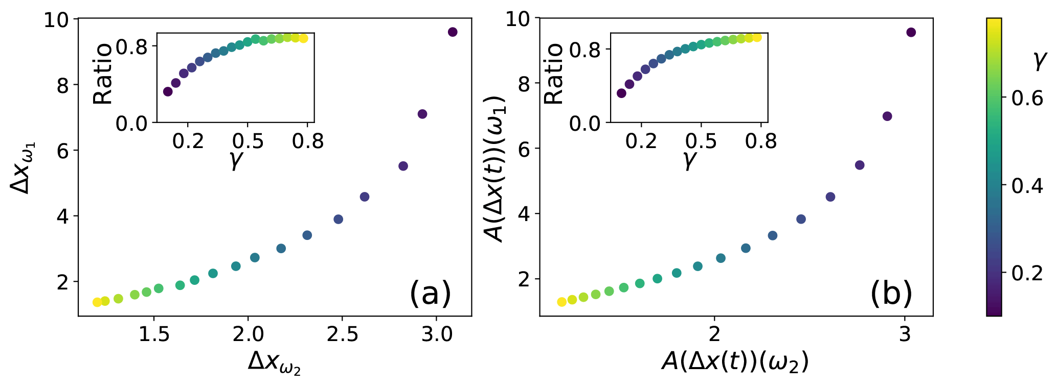
Figure 2(a) Response to forcings at two different frequencies of the one-dimensional Ornstein–Uhlenbeck process. Shown is the average of a 500-member simulation of trajectories. (b) The susceptibility at these frequencies, whose ratio is given in the inset figure. This is an example of a direct dynamical emergent relationship.
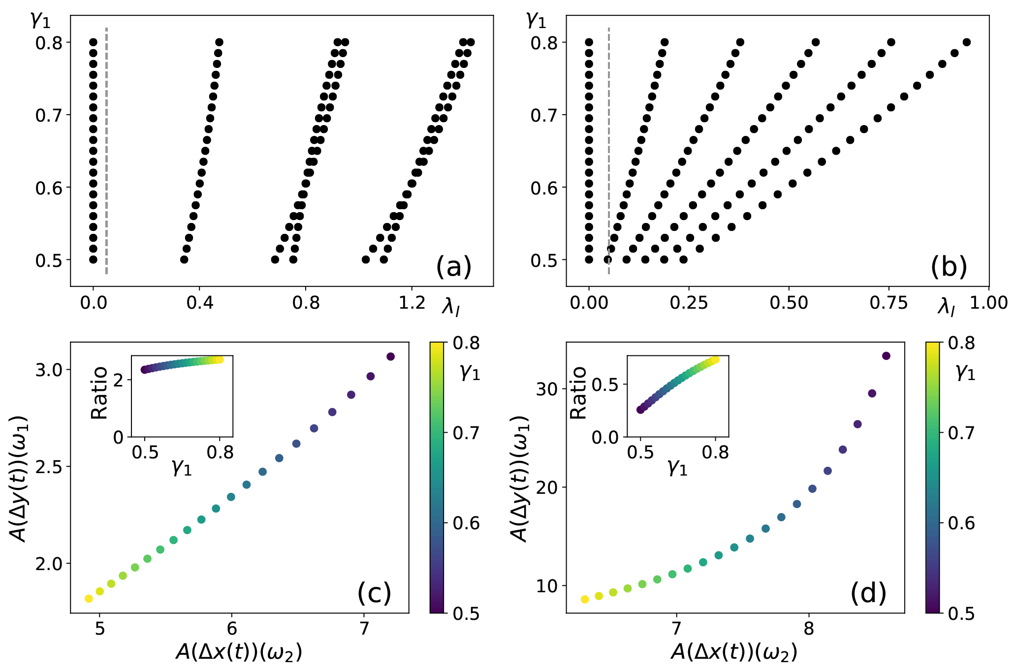
Figure 3Eigenvalue spectrum for (a) δ=0.2 and (b) δ=0.5. The dashed line corresponds to the frequency ω2 of the fast forcing. (c, d) Corresponding susceptibilities, with their ratio in the inset figures. This is an example of an indirect dynamical emergent relationship. Note that for reasons of numerical stability, the range of γ1 is different than that of γ in Fig. 2.
4.1 Ornstein–Uhlenbeck cases
First, the one-dimensional Ornstein–Uhlenbeck process is considered with SDE
forcing Fi(t)=sin2πtωi and frequencies ω1=0.001 and ω2=0.1. A parameter ensemble is created by varying γ. In this case, analytic solutions exist for the eigenvalues and eigenvectors of the generator. Eigenvectors and eigenvalues were determined using the Chang–Cooper scheme on a domain [−25, 25] with Δx=0.25. The numerically computed susceptibilities, as shown in Fig. 2b, are in agreement with the analytic ones and capture the response (Fig. 2a) well, as expected in this linear case.
In the two-dimensional Ornstein–Uhlenbeck case, the same forcing Fi(t) is added but only in the first dimension. The governing SDE is given by
and a parameter ensemble is generated by changing the damping rate γ1. Two ensembles are compared with δ=0.2 in the first ensemble and δ=0.5 in the second. The damping term γ2 is held constant at γ2=0.6.
In Fig. 3, the eigenvalues and susceptibility ratios are plotted. In the case of a relatively weak coupling (δ=0.2), all non-zero eigenvalues are larger than the fast forcing frequency ω2, so the system response time is smaller than the forcing timescales. On the other hand, the strong coupling (δ=0.5) leads to a slowdown of the system, so that some eigenvalues now become smaller than ω2. In these cases (γ1<0.5), the system does not have time to portray the full response to a forcing, while for others (γ1>0.5) it does. Consequently, the strength of the response actually decreases for γ1<0.5. Directly calculating the expectation value as the mean of 500 stochastic trajectories confirms this result (not shown).
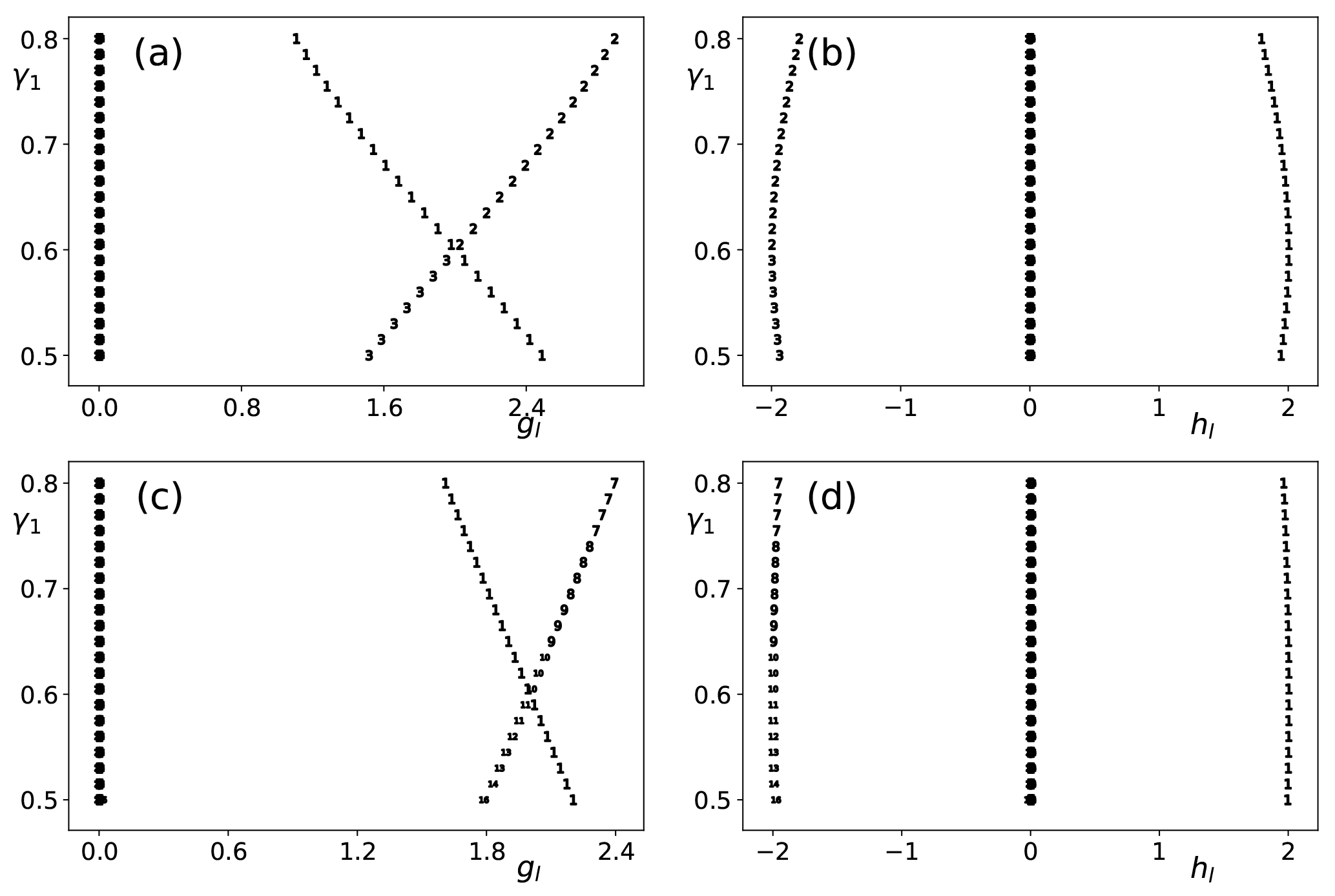
Figure 4(a, b) Projections gl (of predictor variable) and hl (of predictand variable) for a weakly coupled two-dimensional OU system with δ=0.2 and (c, d) the same for δ=0.5.
The results in Fig. 4 show a large variation over the ensemble in the projection term of the predictor on the eigenfunctions (gl; see the Appendix). In contrast, the product of the two projection terms in the predictand (hl) changes relatively little over the ensemble for both coupling strengths. Even though the projection terms now play a significant role in determining the response, the eigenvalues still determine whether the relation is linear (fast compared to forcing) or non-linear (similar size to forcing frequency). In the weak-coupling system, the susceptibility ratio is almost constant, and an emergent linear relationship is found. The strong-coupling system only portrays an emergent relationship for certain regimes (low or high γ1). A case can be made though that the highly coupled system is the system for which finding an emergent constraint is more likely, because the strength of the response is substantially higher and a better signal-to-noise ratio can be obtained.
4.2 Energy balance model
In this section, a specific emergent constraint is examined in more detail, namely the one pertaining to the SAF first described by Hall and Qu (2006). They found a correlation between SAF on a seasonal scale and SAF as a result of climate change. In models with a high snow albedo, the contrast between snow-covered and bare surfaces was largest and consequently the sensitivity to changes in temperature was largest (Qu and Hall, 2007). To study this emergent constraint, we modify a simple energy balance model based on the seminal work by Budyko (1969) and Sellers (1969). The albedo is made temperature dependent following Fraedrich (1979), and a stochastic term is added following Sutera (1981). A parameter in the albedo function will be used to define a parameter ensemble.
With constant albedo, the energy balance model reads
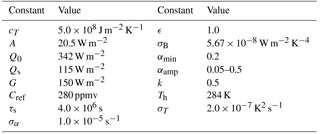
where dT is the temperature change, cT the atmospheric heat capacity, Q the solar insolation, α the albedo, C the concentration of greenhouse gases, Cref a reference concentration, G the radiative forcing due to the reference greenhouse gas concentration, σB the Stefan–Boltzmann constant and ϵ the emissivity of the Earth. The standard parameter values for this model can be found in Table 2. The parameters of the albedo function are chosen to ensure that no bistability is present in the model, in which case LRT would break down.
Before examining the snow-albedo feedback, note that, for some variables, notably the climate sensitivity, a simple energy balance model (EBM) can react differently to forcing from solar insolation or greenhouse gases. This can be determined from, with and for a value of ϵ=1,
Sensitivity to greenhouse forcing decreases when albedo decreases, while sensitivity to solar insolation (seasonal sensitivity) increases for an increasing albedo, using typical values for Q and H.
To mimic the physical mechanism behind the emergent constraint, the albedo is taken to be temperature dependent; i.e. for low (high) temperatures, the albedo is high (low). A logistic function is used to model this effect:
where αmin is the minimum albedo, αamp is the amplitude, k is a steepness factor, and Th is the temperature at which half of the amplitude is reached. The amplitude αamp is the parameter that is varied over the ensemble.
In the first case, the insolation forcing is given by , where τ corresponds to 1 year and Qs is a seasonal modulation amplitude, with parameter values shown in Table 2. The snow-albedo feedback term is then computed by dividing the amplitude of the albedo cycle by the amplitude of the temperature cycle. A second case is considered in which the greenhouse gas concentration C is increased 0.3 % per year from 295 ppmv over a period of 300 years. Here, the snow-albedo feedback is computed by dividing the total albedo response by the total temperature response. In each case, the variance of the noise σT in Eq. (23) was chosen as 10−7 K2 s−1. Changing this parameter does not influence the eigenvalues as expected from the theory (Pavliotis, 2014). While the projections of the eigenvalues and eigenfunctions did change slightly, the susceptibility ratio was not influenced significantly by a variation of the σT (halving and doubling of σ, not shown). In the computation of the solution of the Fokker–Planck equation using the Chang–Cooper scheme, we used a resolution of 1 K which is sufficient to accurately determine the eigenvalues and eigenfunctions of the generator.
As mentioned above, application of Eq. (15) is not self-evident. Considering temperature to be a forcing ignores the fact that temperature responds differently to seasonal and greenhouse gas forcing, as shown in Eq. (25). Secondly, using dα∕dT as the observable directly does not work either. Linear response theory does not give the expectation value of the observable, but the expectation value of the deviation due to the forcing, while we are interested in the change due to a parameter change.
Instead, the SAF can be described by two observables: SAF is determined by taking the ratio of the susceptibilities of albedo to temperature. Therefore, we use the modified Eq. (16):
where
In the case that the susceptibilities are all dominated by one term with index l, this reduces to .
In Fig. 5, the sensitivity of temperature to varying amplitude of the albedo function is shown, as well as the sensitivity of the snow-albedo feedback and condition for the existence of an emergent constraint. As shown in Fig. 5a, no emergent relationship is found for climate sensitivity, a feature that was analytically found in the case of constant albedo. In Fig. 5b, the emergent constraint on SAF is shown. In the warm regime (low albedo, lower line in the figure), the SAF becomes larger for larger αamp. The larger the maximum albedo, the steeper the logistic albedo function. A second effect also takes place, the higher the maximum albedo, the warmer it gets. Consequently, sensitivity of the albedo function is smaller. This decrease in sensitivity also takes place in the cold regime; the colder it gets, the less sensitive the albedo gets. In the cold regime, it is clear that this second mechanism dominates. The results can be reproduced by use of LRT, as shown in Fig. 5c and d. The discrepancies disappear when forcing is small; the climate change forcing in particular is causing most of the differences.
One can extend the energy balance model by representing the response of snow and ice explicitly as a relaxation towards the logistic reference albedo function α(T) given in Eq. (26). This gives the extended model
where s is the response time of the albedo. The drift term in the Fokker–Planck equation corresponding to Eq. (31) is not the gradient of a potential but the eigensolutions of the generator can of course still be computed numerically.
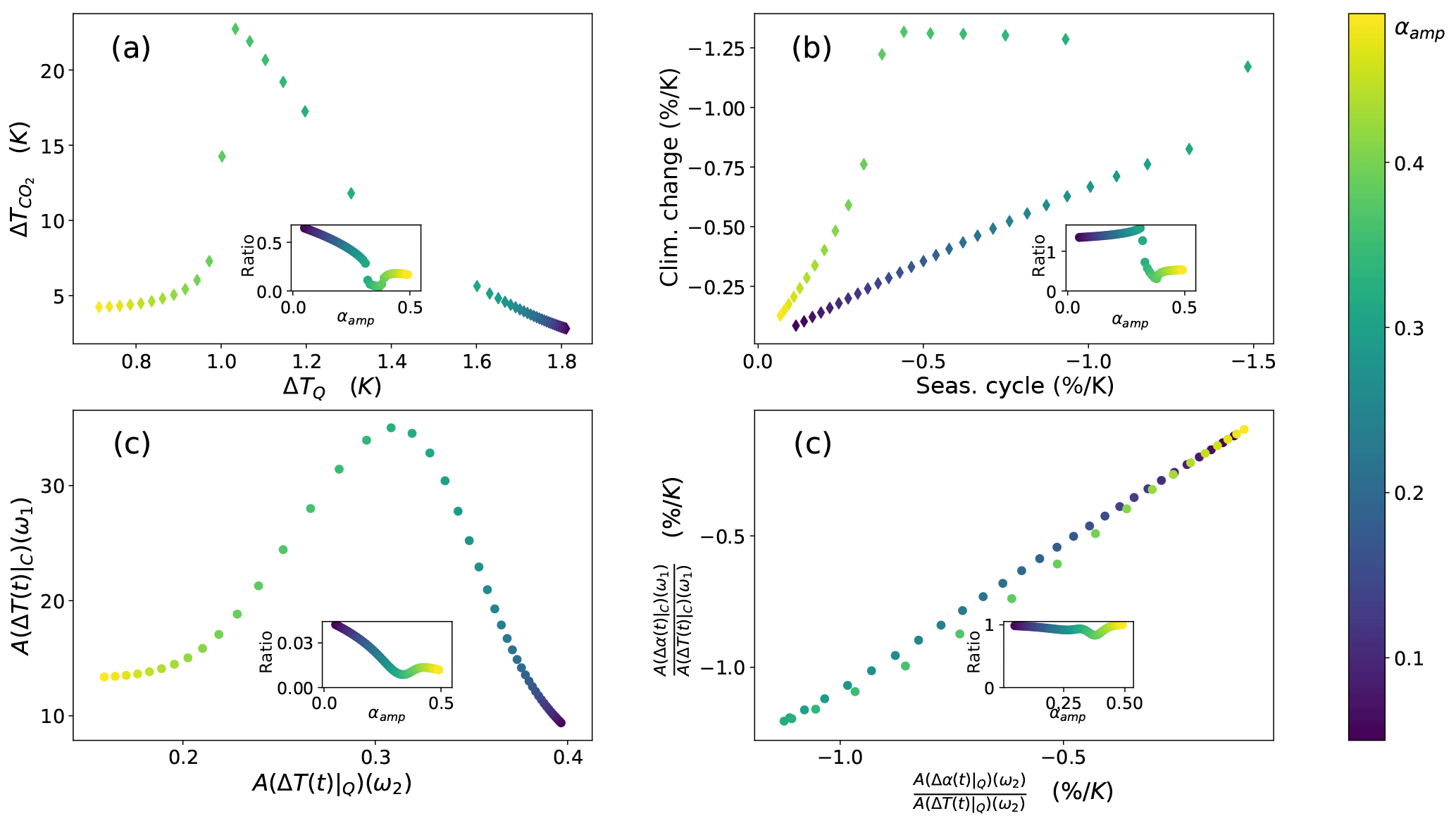
Figure 5(a) The relation between temperature response to the seasonal cycle and the temperature response to greenhouse gas forcing. (b) The strength of the snow-albedo feedback to solar and greenhouse gas forcing on different timescales. In the inset: their ratio as a function of αmax. For clearness, panels (a, b) are shown without noise. (c) The susceptibilities for temperature as the observable. (d) The ratio of albedo and temperature susceptibilities and their ratio (RFS).
Extending the model with an explicit albedo function does not change the dynamics of the system significantly, nor the eigenvalues and eigenvectors. Figure 6b shows the eigenvalues of the extended EBM to be almost exactly equal to the eigenvalues of the original model, the imaginary parts continuing to be zero. The projection coefficients are very similar as well (not shown). Thus, the inclusion of a smaller timescale does not improve the response.
4.3 PlaSim
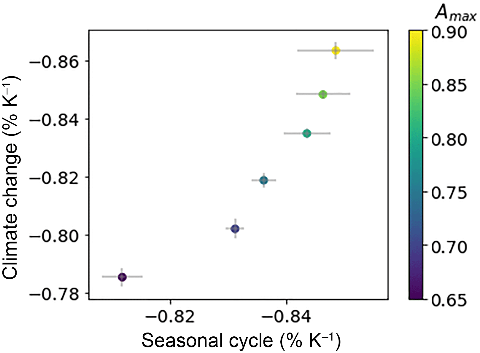
To bridge the gap between parameter ensembles in simple dynamical systems and Earth system models, the SAF emergent constraint is further examined in PlaSim. PlaSim is a numerical model of intermediate complexity, developed at the University of Hamburg to provide a fairly realistic present climate which can still be simulated on a personal computer (Fraedrich et al., 2005). The atmospheric dynamics are modelled using the primitive equations formulated for temperature, vorticity, divergence and surface pressure. Moisture is included by transport of water vapour. The equations are solved using the spectral method. A full set of parameterizations is used for unresolved processes such as long- and shortwave radiation with interactive clouds, boundary layer fluxes of latent and sensible heat and diffusion.
In this climate model, snow albedo is a function of surface temperature Ts, snow depth and vegetation cover. The bare soil snow albedo in PlaSim is described by
This equation is modified in the presence of vegetation and in the case of shallow snow depth; see Lunkeit et al. (2011) for more details. A set of simulations was performed with Amax varying between 0.650 and 0.900. The historical forcing in PlaSim was approximated by a CO2 increase from 295 ppm at a rate of 0.3 % per year in the 20th century and 1 % per year in the 21st century before it stabilized at 720 ppm; a 50-year spin-up corresponding to the period 1850–1900 was used.
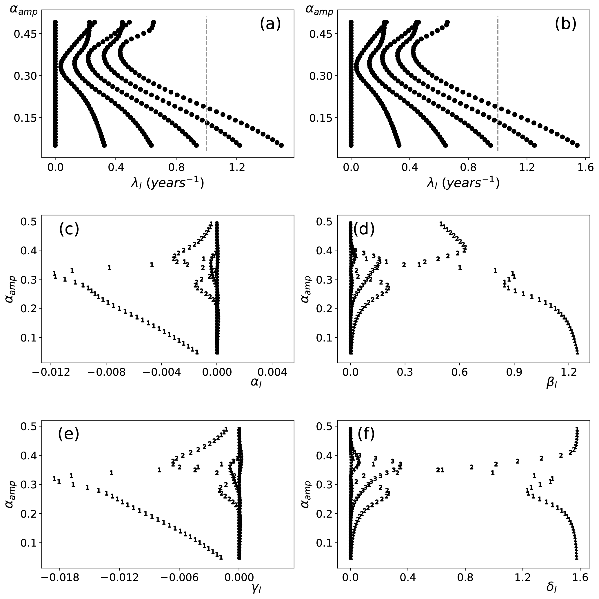
Figure 6(a) Eigenvalues of the EBM depending on the amplitude of the albedo function for the simple EBM. The zero eigenvalues correspond to the invariant measure. (b) The extended EBM. (c) Albedo projection terms for solar forcing (αl) as defined in Eq. (29) where the markers denote l. (d) Same for temperature βl (e, f) projections terms for greenhouse gas forcing γl and δl, respectively.
In Fig. 7, the PlaSim results are shown which can be compared to the results from Hall and Qu (2006) in Fig. 1. Note that the variation in CMIP3 is significantly larger than the variation found in PlaSim but that the PlaSim results fit on the relation found by Hall and Qu (2006). Variations in other parameterizations, such as the maximum snow albedo over forested regions, increase the spread in PlaSim SAF further (not shown). This simulation shows that the constraint that emerges in a multi-model ensemble with structurally different formulations of the snow response can to some extent also be reproduced using variations in one parameter. This provides the justification for simplifying further to energy balance models to examine the SAF emergent constraint.
In this paper, we have presented a dynamical framework behind the occurrence of emergent constraints in parameter-dependent stochastic dynamical systems. In these systems, emergent constraints are related to ratios of response functions which can be determined using linear response theory. It was shown that for a large class of systems, these ratios could be expressed in terms of eigenvalues and projections on eigenvectors of the generator of the system.
A classification of emergent constraints was given and several types could be distinguished depending on whether similar (direct) or different (indirect) observables are considered and whether a response in present-day climate (dynamical) or the time-independent part of present-day climate (static) is linked to a response of the future climate system. For a linear dynamical emergent constraint, the ratio of susceptibilities at the two frequencies under consideration should be a positive constant over the ensemble. When the response is computed with respect to an internal variable (in contrast to an external forcing), a condition is posed on the susceptibilities of the two observables in the system. Static constraints are encountered when a linear relationship is found between the expectation value of the observable and the susceptibility at the frequency of the forcing.
Examples were given using several idealized climate models. In particular, the emergent constraints involving the snow-albedo feedback was considered in detail. We found that linear dynamical emergent relationships can occur when the timescale of the system, indicated by the eigenvalues, changes with the parameter and is smaller than the forcing timescales. This is of particular interest because differences in response size between climate models is often determined by feedback strength in climate systems. Larger feedbacks give rise to larger timescales (Roe, 2009), which is reflected in the eigenvalues of the generator. For an emergent constraint on a feedback quantity, a more complicated constraint mechanism occurs, where one has to take into account the response to two different observables, which typically have different timescales. When the condition of the predictor's timescale being smaller than the forcing timescale is not met, deviations from linearity occur. When the linearity of the relation is exploited in further analysis, such as in the interpretation of emergent constraints by Wenzel et al. (2014), this might lead to a bias in the estimate of the predictand.
Modelling emergent constraints with conceptual models is justified when different Earth system models (ESMs) are closely related and structural differences can be parameterized. This can, for instance, be tested using an intermediate complexity model with full parameterization of the process under consideration.
The classification of emergent constraints provided gives a hint to which kind of emergent constraints one can look out for in an ensemble of high-dimensional global climate models (GCMs). To find an emergent constraint for climate sensitivity by data mining in a CMIP5 ensemble proved fruitless (Caldwell et al., 2014). Using the susceptibilities to find new emergent constraints does not seem to have a direct advantage above directly looking for plausible correlations, but susceptibilities might provide additional information. For example, when a susceptibility shows a resonance at a certain frequency over the ensemble of models, this could suggest that the same feedback is present in all simulations.
In a high-dimensional dynamical system, eigenfunctions and eigenvalues can be accessed with the help of transfer operators, associated with the propagation of probability densities associated with the Fokker–Planck operator. The eigenfunctions that lie on the invariant measure are then computed by making use of the ergodic properties of the climate system. To overcome the burden of high dimensionality, a reduced transfer operator can be computed from a very long simulation, from which the eigenfunctions on the attractor are approximated (Tantet, 2016). However, a forcing on the system does not generally lie only on the attractor and should be split into a part parallel and perpendicular to the attractor. Consequently, the eigenvectors off the attractor cannot a priori be ignored (Lucarini and Sarno, 2011). Gritsun and Lucarini (2017) showed that indeed for some geophysical systems, specifically quasi-geostrophic flow with orographic forcing, the response to the forcing may have no resemblance to the unforced variability in the same range of spatial and temporal scales.
In conclusion, while the current theoretical framework provides an understanding on how emergent constraints may arise in low-dimensional stochastic dynamical systems, its application to output from GCMs, in particular in finding novel and useful emergent constraints, is a challenging issue for future work.
All the code used in this paper is available upon request.
For A=x, we find from Eq. (5) that
Using the expression for the equilibrium solution from Eq. (3), we find
and hence Eq. (33) becomes
With the standard L2 inner product, the adjoint of ℒ determined as , where ℒ is the generator of the OU process, is given by
Using this property in Eq. (35), we find
and hence
Next, an inner product is defined as
As a next step, let λl and ϕl be the eigenvalues of the generator, i.e. solutions v of
For reversible processes, these eigenvalues are real, positive and discrete under the inner product . The eigenfunctions form a complete orthonormal basis, such that (Pavliotis, 2014). Now, eℒt(x) represents solutions u(x, t) of the problem
with initial condition . We can expand u into eigenfunctions as
From the initial condition, we find
and using the orthogonality of the ϕl under the inner product , we find
On the other hand, substituting the expression for u into Eq. (38) gives
where
Repeating the derivation with a general observable A=f(x) gives . The first term in βl denotes the projection of the observable on the eigenfunctions and could intuitively be interpreted (for l>0) as the amenability of the observable to change. The second projection term in βl can be understood to be the amenability of the whole system to change under the influence of the forcing field. In Eq. (12), those observables are Y1 and Y2, so that and .
FJMMN and HAD designed the study, FJMMN performed the numerical calculations and drafted the manuscript. HAD supervised the project. Both authors discussed the results and contributed to the final manuscript.
The authors declare that they have no conflict of interest.
We thank Frank Lunkeit for his help with the PlaSim simulations and
Alexis Tantet is thanked for useful discussions. The authors also thank
Valerio Lucarini and an anonymous reviewer whose suggestions helped improve
and clarify the manuscript. Both authors acknowledge support by the
Netherlands Earth System Science Centre (NESSC), financially supported by the
Ministry of Education, Culture and Science (OCW), grant no. 024.002.001.
Edited by: Andrey Gritsun
Reviewed by: Valerio Lucarini and one anonymous referee
Allen, M. R. and Ingram, W. J.: Constraints on future changes in climate and the hydrologic cycle, Nature, 419, 224–232, https://doi.org/10.1038/nature01092, 2002. a
Boe, J., Hall, A., and Qu, X.: September sea-ice cover in the Arctic Ocean projected to vanish by 2100, Nat. Geosci., 2, 341–343, 2009. a
Bracegirdle, T. J. and Stephenson, D. B.: On the Robustness of Emergent Constraints Used in Multimodel Climate Change Projections of Arctic Warming, J. Climate, 26, 669–678, 2013. a, b, c, d
Budyko, M. I.: The effect of solar variations on the climate of the Earth, Tellus, 7, 611–619, https://doi.org/10.1111/j.2153-3490.1969.tb00466.x, 1969. a
Caldwell, P. M., Bretherton, C. S., Zelinka, M. D., Klein, S. A., Santer, B. D., and Sanderson, B. M.: Statistical significance of climate sensitivity predictors obtained by data mining, Geophys. Res. Lett., 41, 1803–1808, 2014. a
Chang, J. and Cooper, G.: A practical difference scheme for Fokker–Planck equations, J. Comput. Phys., 6, 1–16, 1970. a
Clement, A. C., Burgman, R., and Norris, J. R.: Observational and Model Evidence for Positive Low-Level Cloud Feedback, Science, 325, 460–464, 2009. a
Collins, M., Chandler, R. E., Cox, P. M., Huthnance, J. M., Rougier, J., and Stephenson, D. B.: Quantifying future climate change, Nat. Clim. Change, 2, 403–409, https://doi.org/10.1038/nclimate1414, 2012. a
Cox, P. M., Huntingford, C., and Williamson, M. S.: Emergent constraint on equilibrium climate sensitivity from global temperature variability, Nature, 553, 319–322, https://doi.org/10.1038/nature25450, 2018. a, b, c
Fasullo, J. T. and Trenberth, K. E.: A Less Cloudy Future: The Role of Subtropical Subsidence in Climate Sensitivity, Science, 338, 792–794, 2012. a
Fraedrich, K.: Catastrophes and resilience of a zero-dimensional climate system with ice-albedo and greenhouse feedback, Q. J. Roy. Meteorol. Soc., 105, 147–167, https://doi.org/10.1002/qj.49710544310, 1979. a
Fraedrich, K., Jansen, H., Kusch, U., and Lunkeit, F.: The Planet Simulator: Towards a user friendly model, Meteorol. Z., 14, 299–304, 2005. a
Gordon, N. D. and Klein, S. A.: Low-cloud optical depth feedback in climate models, J. Geophys. Res.-Atmos., 119, 6052–6065, 2014. a
Grise, K. M., Polvani, L. M., and Fasullo, J. T.: Reexamining the Relationship between Climate Sensitivity and the Southern Hemisphere Radiation Budget in CMIP Models, J. Climate, 28, 9298–9312, 2015. a
Gritsun, A. and Lucarini, V.: Fluctuations, response, and resonances in a simple atmospheric model, Physica D, 349, 62–76, 2017. a
Hairer, M. and Majda, A. J.: A simple framework to justify linear response theory, Nonlinearity, 23, 909–922, https://doi.org/10.1088/0951-7715/23/4/008, 2010. a
Hall, A. and Qu, X.: Using the current seasonal cycle to constrain snow albedo feedback in future climate change, Geophys. Res. Lett., 33, l03502, https://doi.org/10.1029/2005GL025127, 2006. a, b, c, d, e, f, g, h
Klein, S. A. and Hall, A.: Emergent Constraints for Cloud Feedbacks, Current Clim. Change Rep., 1, 276–287, 2015. a
Kloeden, P. and Platen, E.: Numerical Solution of Stochastic Differential Equations, Stochastic Modelling and Applied Probability, Springer, Berlin, Heidelberg, 1992. a
Knutti, R., Meehl, G. A., Allen, M. R., and Stainforth, D. A.: Constraining Climate Sensitivity from the Seasonal Cycle in Surface Temperature, J. Climate, 19, 4224–4233, https://doi.org/10.1175/JCLI3865.1, 2006. a
Kwiatkowski, L., Bopp, L., Aumont, O., Ciais, P., Cox, P. M., Laufkötter, C., Li, Y., and Séférian, R.: Emergent constraints on projections of declining primary production in the tropical oceans, Nat. Clim. Change, 7, 355–358, 2017. a
Lehoucq, R. B., Sorensen, D. C., and Yang, C.: ARPACK USERS GUIDE: Solution of Large Scale Eigenvalue Problems by Implicitly Restarted Arnoldi Methods, SIAM, Philadelphia, 1998. a
Lucarini, V. and Sarno, S.: A statistical mechanical approach for the computation of the climatic response to general forcings, Nonlin. Process. Geophys., 18, 7–28, https://doi.org/10.5194/npg-18-7-2011, 2011. a, b, c
Lunkeit, F., Borth, H., Böttinger, M., and Fraedlich, F.: PLASIM Reference Manual, version 16, available at: https://www.mi.uni-hamburg.de/en/arbeitsgruppen/theoretische-meteorologie/modelle/sources/psreferencemanual-1.pdf (last access: 1 April 2017), 2011. a
Pavliotis, G. A.: Stochastic Processes and Applications: Diffusion Processes, the Fokker–Planck and Langevin Equations, Springer, New York, NY, https://doi.org/10.1007/978-1-4939-1323-7_4, 2014. a, b, c, d, e
Qu, X. and Hall, A.: What Controls the Strength of Snow-Albedo Feedback?, J. Climate, 20, 3971–3981, 2007. a, b
Qu, X. and Hall, A.: On the persistent spread in snow-albedo feedback, Clim. Dynam., 42, 69–81, https://doi.org/10.1007/s00382-013-1774-0, 2014. a
Qu, X., Hall, A., Klein, S. A., and Caldwell, P. M.: On the spread of changes in marine low cloud cover in climate model simulations of the 21st century, Clim. Dynam., 42, 2603–2626, https://doi.org/10.1007/s00382-013-1945-z, 2014. a
Ragone, F., Lucarini, V., and Lunkeit, F.: A new framework for climate sensitivity and prediction: a modelling perspective, Clim. Dynam., 46, 1459–1471, https://doi.org/10.1007/s00382-015-2657-3, 2016. a, b
Risken, H.: The Fokker–Planck Equation, in: vol. 5 of Springer Series in Synergetics, SpringerLink, Berlin, 1996. a
Roe, G.: Feedbacks, Timescales, and Seeing Red, Annu. Rev. Earth Planet. Sci., 37, 93–115, https://doi.org/10.1146/annurev.earth.061008.134734, 2009. a
Ruelle, D.: General linear response formula in statistical mechanics, and the fluctuation-dissipation theorem far from equilibrium, Phys. Lett. A, 245, 220–224, https://doi.org/10.1016/S0375-9601(98)00419-8, 1998. a
Ruelle, D.: A review of linear response theory for general differentiable dynamical systems, Nonlinearity, 22, 855–870, 2009. a
Sellers, W. D.: A Global Climatic Model Based on the Energy Balance of the Earth–Atmosphere System, J. Appl. Meteorol., 8, 392–400, https://doi.org/10.1175/1520-0450(1969)008<0392:AGCMBO>2.0.CO;2, 1969. a
Sherwood, S. C., Bony, S., and Dufresne, J.-L.: Spread in model climate sensitivity traced to atmospheric convective mixing, Nature, 505, 37–42, https://doi.org/10.1038/nature12829, 2014. a
Su, H., Jiang, J. H., Zhai, C., Shen, T. J., Neelin, J. D., Stephens, G. L., and Yung, Y. L.: Weakening and strengthening structures in the Hadley Circulation change under global warming and implications for cloud response and climate sensitivity, J. Geophys. Res.-Atmos., 119, 5787–5805, 2014. a
Sutera, A.: On stochastic perturbation and long-term climate behaviour, Q. J. Roy. Meteorol. Soc., 107, 137–151, https://doi.org/10.1002/qj.49710745109, 1981. a
Tantet, A.: Ergodic theory of climate: variability, stability and response, PhD thesis, Utrecht University, Utrecht, 2016. a
Tian, B.: Spread of model climate sensitivity linked to double-Intertropical Convergence Zone bias, Geophys. Res. Lett., 42, 4133–4141, https://doi.org/10.1002/2015GL064119, 2015. a, b
Trenberth, K. E. and Fasullo, J. T.: Simulation of Present-Day and Twenty-First-Century Energy Budgets of the Southern Oceans, J. Climate, 23, 440–454, 2010. a, b
Wenzel, S., Cox, P. M., Eyring, V., and Friedlingstein, P.: Emergent constraints on climate-carbon cycle feedbacks in the CMIP5 Earth system models, J. Geophys. Res.-Biogeo., 119, 794–807, https://doi.org/10.1002/2013JG002591, 2014. a, b, c
emergent constraintsuses observations of current climate to improve those predictions, using relationships between different climate models. Our paper first classifies the different uses of the technique, and continues with proposing a mathematical justification for their use. We also highlight when the application of emergent constraints might give biased predictions.