Seasonal prediction skill of East Asian summer monsoon in CMIP5 models

The East Asian summer monsoon (EASM) is an important part of the global climate system and plays a vital role in the Asian climate. Its seasonal predictability is a long-standing issue within the monsoon scientist community. In this study, we analyse the seasonal (the leading time is at least 6 months) prediction skill of the EASM rainfall and its associated general circulation in non-initialised and initialised simulations for the years 1979–2005, which are performed by six prediction systems (i.e. the BCC-CSM1-1, the CanCM4, the GFDL-CM2p1, the HadCM3, the MIROC5, and the MPI-ESM-LR) from the Coupled Model Intercomparison Project phase 5 (CMIP 5). We find that most prediction systems of simulated zonal wind over 850 and 200 hPa are significantly improved in the initialised simulations compared to non-initialised simulations. Based on the knowledge that zonal wind indices can be used as potential predictors for the EASM, we select an EASM index based upon the zonal wind over 850 hPa for further analysis. This assessment shows that the GFDL-CM2p1 and the MIROC5 added prediction skill in simulating the EASM index with initialisation, the BCC-CSM1-1, the CanCM4, and the MPI-ESM-LR changed the skill insignificantly, and the HadCM3 indicates a decreased skill score. The different responses to initialisation can be traced back to the ability of the models to capture the ENSO (El Niño–Southern Oscillation) and EASM coupled mode, particularly the Southern Oscillation–EASM coupled mode. As is known from observation studies, this mode links the oceanic circulation and the EASM rainfall. Overall, the GFDL-CM2p1 and the MIROC5 are capable of predicting the EASM on a seasonal timescale under the current initialisation strategy.

1 Introduction

The Asian monsoon is the most powerful monsoon system in the world due to the thermal contrast between the Eurasian continent and the Indo-Pacific Ocean. Its evolution and variability critically influence the livelihood and the socio-economic status of over 2 billion people who live in the Asian-monsoon-dominated region. It encompasses two sub-monsoon systems, the South Asian monsoon (SAM) and the East Asian monsoon (EAM; Wang, 2006). In summertime (June–July–August), the EAM, namely the East Asian summer monsoon (EASM), occurs from the Indo-China peninsula to the Korean Peninsula and Japan and shows strong intraseasonal-to-interdecadal variability (Ding and Chan, 2005). Thus, an accurate prediction of the EASM is an important and long-standing issue in climate science.

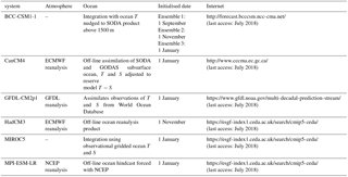
Table 1 Details of the prediction systems investigated in this study.

To predict the EASM, there are two approaches: statistical prediction and dynamical prediction. The statistical method seeks the relationship between the EASM and a strong climate signal (e.g. ENSO, NAO; Wu et al., 2009; Yim et al., 2014; Wang et al., 2015). This method establishes an empirical equation between the EASM and climate index. However, it is limited by the strength of the climate signal. The other method is dynamical prediction. It employs a climate model to predict the EASM (Sperber et al., 2001; Kang and Yoo, 2006; Wang et al., 2008a; Yang et al., 2008; Lee et al., 2010; Kim et al., 2012). Without initialisation, both atmosphere general circulation models (AGCMs) and coupled atmosphere–ocean general circulation models (CGCMs) cannot predict the climate on a seasonal timescale (Goddard et al., 2001). Given an initial condition, AGCMs have the ability to predict the climate, but show little skill in predicting the EASM (Wang et al., 2005; Barnston et al., 2010). Because AGCMs fail to produce a correct relationship between the EASM and the sea surface temperature (SST) anomalies over the tropical western North Pacific, the South China Sea, and the Bay of Bengal (Wang et al., 2004, 2005), the monsoon community endeavours to predict the EASM with CGCMs (Wang et al., 2008a; Zhou et al., 2009; Kim et al., 2012; Jiang et al., 2013).

CGCMs have proved to be the most valuable tools in predicting the EASM (Wang et al., 2008a; Zhou et al., 2009; Kim et al., 2012; Jiang et al., 2013). However, the performance of CGCMs in predicting the EASM on seasonal timescales strongly depends on their ability to reproduce the air–sea coupled process (Kug et al., 2008) and on the given initial conditions (Wang et al., 2005). In the Coupled Model Intercomparison Project (CMIP) phase 3 (CMIP3; Meehl et al., 2007) era, the models simulate not only a too-weak tropical SST–monsoon teleconnection (Kim et al., 2008, 2011), but also a too-weak East Asian zonal wind–rainfall teleconnection (Sperber et al., 2013). Compared to CMIP3 models, CMIP phase 5 (CMIP5; Taylor et al., 2012) models improve the representation of monsoon status (Sperber et al., 2013). Therefore, given the initial conditions, the CMIP5 models do have the potential to predict the EASM.

Table 2 Brief summaries of initialisation strategies used by modelling groups in the study. ECMWF: European Centre for Medium-Range Weather Forecasts; GODAS: Global Ocean Data Assimilation System; NCEP: National Centers for Environmental Prediction; S: salinity; SODA: Simple Ocean Data Assimilation; T: temperature. Initialised date shows the first initialised day of every prediction year.

As mentioned, initial conditions play a vital factor in predicting the EASM on a sub-seasonal to seasonal timescale (Wang et al., 2005; Kang and Shukla, 2006). Under the current set-up of initialisation, the CMIP5 models show the ability to predict the SST variation index (i.e. El Niño–Southern Oscillation (ENSO) index; Niño3.4) up to 15 months in advance (Meehl and Teng, 2012; Meehl et al., 2014; Choi et al., 2016). This extended prediction skill of the ENSO suggests that the EASM can be predicted on a seasonal timescale if the dynamical link between the ENSO and monsoon circulations is well represented in these models. Two scientific questions will be addressed in this study: (1) how realistic are the initialised CMIP5 models in representing the EASM? (2) Can the CMIP5 models capture the dynamical link between the ENSO and EASM?

In this paper, we will intercompare the influence of the initialisation on the capability of the CMIP5 models to capture the EASM and the ENSO–EASM teleconnections. The model simulations, comparison data, and methods are introduced in Sect. 2. Section 3 describes the seasonal skill of the rainfall predictions and the prediction of the associated general circulation of the EASM. The mechanism causing the differential response of the models to the initialisation is presented in Sect. 4. The discussions are presented in Sect. 5. Section 6 summarises the findings of this paper.

2 Models, data, and methods

2.1 Models and initialisation

In this study, we evaluate six prediction systems from the CMIP5 project (Table 1) which have performed a yearly initialisation (Meehl et al., 2014). Their simulations can be used in seasonal prediction studies. There are two groups of experiments: without initialisation (non-initialisation) and with initialisation. For non-initialised simulations, the models are forced by observed atmospheric composition changes (reflecting both anthropogenic and natural sources) and, for the first time, including the time-evolving land cover (Taylor et al., 2012). For initialised simulations, the models update the time-evolving observed atmospheric and oceanic component (Taylor et al., 2012). Following the CMIP5 framework, the six models establish their initialisation strategies, which are summarised in Table 2. More details about the initialisation strategy of each model can be found in the reference paper in Table 1. To simplify the comparison, we select the first lead year (up to 12 months) results for further analysis. The HadCM3-ff is the full-field initialised simulation, which employs the same CGCM (HadCM3) as the anomaly initialisation. Satellite era (1979 to 2005) simulations are used in the study due to the spatial coverage of precipitation observations.

The six models employ different initialisation strategies for atmospheric and oceanic process and for initial date (Table 2). These initialisation strategies contribute to a new approach for climate prediction on a decadal timescale (Meehl et al., 2014). As the ocean is driving the long-term prediction skill rather than the initial condition of the atmosphere, the timing of the initialisation has to be considered on the timescale of the ocean circulation, i.e. years to decades. On an ocean timescale, the initialisation takes place with comparable timing and therefore the results are comparable. This approach is based on decadal prediction experiments, which deviates from the scores of other seasonal prediction experiments based on initialisation techniques derived from weather forecasting.

2.2 Comparison data

The main datasets used for comparison in this study include the following: (1) monthly precipitation data from the Global Precipitation Climatology Project (GPCP; Adler et al., 2003); (2) monthly circulation data from the ECMWF Interim reanalysis (ERA-Interim; Dee et al., 2011); and (3) monthly mean SST from the National Oceanic and Atmospheric Administration (NOAA) improved Extended Reconstructed SST version 4 (ERSST v4; Huang et al., 2015). All the model data and the comparison data are remapped onto a common grid of 2.5^∘ × 2.5^∘ by bilinear interpolation to reduce the uncertainty induced by different data resolutions.

2.3 East Asian monsoon index and ENSO index

In recent decades, more than 25 general circulation indices have been produced to define the variability and the long-term change in the EASM. Wang et al. (2008b) arranged the 25 monsoon indices according to their ability to capture the main features of the EASM. The Wang and Fan index (hereafter WF index; 1999) shows the best performance in capturing the total variance in precipitation and three-dimensional circulation over East Asia. We thus select the WF index for further analysis. Its definition is a standardised average zonal wind over 850 hPa at 5^∘–15^∘ N, 90^∘–130^∘ E subtracting at 22.5^∘–32.5^∘ N, 110^∘–140^∘ E. The WF index is a shear vorticity index which is described by a north–south gradient of the zonal winds. In the positive (negative) phase of the WF index years, two strong (weak) rainfall belts are located at the Indo-China peninsula to the Philippine Sea and northern China to the Japanese Sea, and a weak (strong) rainfall belt occurs from the Yangtze River basin to the south of Japan. The average summer (June–July–August) WF index is used to represent the EASM for further analysis in this study.

Here, we choose the Niño3.4 and Southern Oscillation index (SOI) to represent the ENSO status. The Niño3.4 is calculated by the SST anomaly in the central Pacific (190–240^∘ E, 5^∘ S–5^∘ N), while the SOI is based upon the anomaly of the sea level pressure differences between Tahiti (210.75^∘ E, 17.6^∘ S) and Darwin (130.83^∘ E, 12.5^∘ S). To calculate the SOI, we interpolate the grid data to the Tahiti and the Darwin point by bilinear interpolation.

2.4 Methods

In this study, we employ the un-centred pattern correlation coefficient (PCC; for more details see Barnett and Schlesinger, 1987) to analyse the model performance in comparison to the observational data because centred correlations alone are not sufficient for the attribution of seasonal prediction (Mitchell et al., 2001). The un-centred PCC is defined by

$$\begin{array}{}\text{(1)}& {\displaystyle }\text{PCC}={\displaystyle \frac{{\sum }_{x=\mathrm{1}}^n{\sum }_{y=\mathrm{1}}^m{w}_{(x,y)}{F}_{(x,y)}{A}_{(x,y)}}{\sqrt{{\sum }_{x=\mathrm{1}}^n{\sum }_{y=\mathrm{1}}^m{F}_{(x,y)}^{\mathrm{2}}{\sum }_{x=\mathrm{1}}^n{\sum }_{y=\mathrm{1}}^m{w}_{(x,y)}{A}_{(x,y)}^{\mathrm{2}}}}},\end{array}$$

where n and m are grids on longitude and latitude, respectively. F_(x,y) and A_(x,y) represent two dimensions comparing and validating value. w_(x,y) indicates the weighting coefficient for each grid. An equal weighting coefficient was applied in the study area.

We also use the anomaly correlation coefficient (ACC) to analyse the model performance in reproducing observational variations. The ACC is the correlation between anomalies of forecasts and those of verifying values with the reference values, such as climatological values (Drosdowsky and Zhang, 2003). Its definition is

$$\begin{array}{ll}{\displaystyle }\text{ACC}=& {\displaystyle \frac{{\sum }_{x=\mathrm{1}}^n{w}_i\left(f_i-\stackrel{\mathrm{‾}}{f}\right)\left(a_i-\stackrel{\mathrm{‾}}{a}\right)}{\sqrt{{\sum }_{i=\mathrm{1}}^n{w}_i{\left(f_i-\stackrel{\mathrm{‾}}{f}\right)}^{\mathrm{2}}{\sum }_{i=\mathrm{1}}^n{w}_i{\left(a_i-\stackrel{\mathrm{‾}}{a}\right)}^{\mathrm{2}}}}},\\ \text{(2)}& {\displaystyle }& {\displaystyle }(-\mathrm{1}\le \text{ACC}\le \mathrm{1})\end{array}$$

$$\begin{array}{}\text{(3)}& {\displaystyle }& {\displaystyle }{f}_i=F_i-C_i,\stackrel{\mathrm{‾}}{f}\left(\sum _{i=\mathrm{1}}^n{w}_i{f}_i\right)/\sum _{i=\mathrm{1}}^n{w}_i,\text{(4)}& {\displaystyle }& {\displaystyle }{a}_i=A_i-C_i,\stackrel{\mathrm{‾}}{a}\left(\sum _{i=\mathrm{1}}^n{w}_i{a}_i\right)/\sum _{i=\mathrm{1}}^n{w}_i,\end{array}$$

where n is the number of samples, and F_i, A_i, and C_i represent comparison, verifying value, and reference value such as climatological value, respectively. Also, $\stackrel{\mathrm{‾}}{f}$ is the mean of f_i, $\stackrel{\mathrm{‾}}{a}$ is the mean of a_i, and w_i indicates the weighting coefficient. If the variation in anomalies of comparison is coincident with that of the anomalies of verifying value, ACC will be 1 (the maximum value). It indicates that the forecast has good skill.

The root mean square error (RMSE) is employed to check the model deviation from the observation and its definition is

$$\begin{array}{}\text{(5)}& {\displaystyle }{\displaystyle }\text{RMSE}=\sqrt{\sum _{i=\mathrm{1}}^n{w}_i{D}_i^{\mathrm{2}}}/\sqrt{\sum _{i=\mathrm{1}}^n{w}_i},\end{array}$$

where D_i represents the deviation between comparison and verifying value, w_i is the weighting coefficient for each sample, and n is the number of samples. If RMSE is closer to zero, it means that the comparisons are closer to the verifying values.

3 Seasonal prediction skill of the EASM

The EASM has complex spatial and temporal structures that encompass the tropics, subtropics, and mid-latitudes (Tao and Chen, 1987; Ding, 1994). In the late spring, an enhanced rainfall pattern is observed in the Indo-China peninsula and in the South China Sea. At the same time, the rainfall belt advances northwards to the south of China. In the early summer, the rainfall occurs in the Yangtze River basin and in southern Japan; these are called the Meiyu and Baiu seasons, respectively. The rainfall belt can reach as far as northern China, the Korean Peninsula (called the Changma rainy season), and central Japan in July (Ding, 2004; Ding and Chan, 2005).

The EASM is characterised by both seasonal heterogeneous rainfall distribution and associated large-scale circulation systems (Wang et al., 2008b). In the summer season, water moisture migrates from the Pacific Ocean to central and eastern Asia, which is carried by the south-west surface winds. Generally, a strong summer monsoon year is followed by precipitation in northern China, while a weak summer monsoon year is usually accompanied by heavier rainfall along the Yangtze River basin (Ding, 1994; Zhou and Yu, 2005).

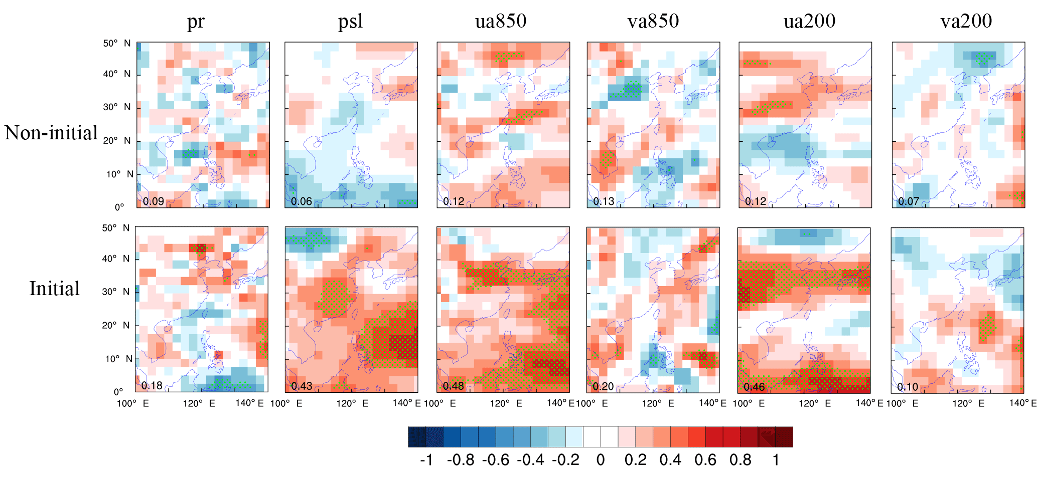
Figure 1 Anomaly correlation coefficient of six variables (i.e. precipitation, mean sea level pressure, and winds over 850 and 200 hPa) between multi-model ensemble mean and observations in non-initialisation and initialisation. The green dotted grids illustrate the significance level at 0.05. The number in the lower left corner indicates the ratio of significant grid points to entire grids. The GPCP is employed as the reference data for precipitation (pr), while winds (i.e. ua850, va850, ua200, and va200) and mean sea level pressure (psl) are compared with ERA-Interim reanalysis.

Table 3 Description of the six variables which contribute to the EASM. The abbreviation of these variables follows the guidelines of CMIP5.

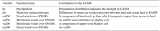
For multi-model ensemble mean (MME), the prediction skill of the June–July–August mean rainfall and the associated general circulation variable (i.e. zonal and meridional wind and mean sea level pressure) are presented in Fig. 1. These variables have been widely used to calculate the monsoon index (Wang et al., 2008b). Table 3 shows the contribution of these variables to the EASM. Their abbreviations follow the guidelines of CMIP5 (Taylor et al., 2012). Compared to the non-initialised experiment, a larger predicted area can be found in the initialised experiment, especially for the psl, ua850, and ua200. There are small changes to the predicted area between the non-initialised and initialised experiment for the pr, va850, and va200. The individual model shows an acceptable performance (high PCC) in capturing the observed spatial variation of the six variables, but a poor performance in simulating their temporal variation (with low ACC; Fig. 2). There is no improvement in estimating the spatial variation of the six variables with initialisation. We can see that the models show a higher ACC in the initialised simulations than that in the non-initialised ones. The improvement in simulating the temporal variation of zonal winds (i.e. ua850 and ua200) is larger than that for the rainfall and meridional winds. One can exploit this improvement by using a general-circulation-based monsoon index as a tool to predict the EASM. As mentioned in Sect. 2.3, the WF index better represents the monsoon rainfall and its associated general circulation structure than the other monsoon index. Therefore, the prediction skill of EASM in the following analysis is based on the WF index.

Figure 2 Taylor diagrams displaying the pattern (PCC) and temporal (ACC) correlation metrics of six variables between observation and model simulation in the EASM region (0–50^∘ N, 100–140^∘ E). Each coloured marker represents a model, i.e. the BCC-CSM1-1 (black), the CanCM4 (green), the GFDL-CM2p1 (red), the HadCM3 (blue), the MIROC5 (brown), the MPI-ESM-LR (light blue), and the HadCM3-ff (orange). The grey marker indicates the multi-model mean (MME).

In non-initialised simulations, none of the models capture the observed EASM, as indicated by an insignificant ACC (Fig. 3). The CanCM4 and the GFDL-CM2p1 simulate a negative phase, while the BCC-CSM1-1, the HadCM3, the MIROC5, and the MPI-ESM-LR all predicted a positive phase of the EASM. With initialisation, the GFDL-CM2p1 and the MIROC5 improve the skill to simulate the EASM, the CanCM4 and the MPI-ESM-LR displayed hardly any reaction, while the BCC-CSM1-1 and the HadCM3 show a worse performance than without initialisation. Particularly with anomaly initialisation, the HadCM3 significantly lost its prediction skill in capturing the EASM. The CMIP5 models show different responses to the initialisation in predicting the EASM on a seasonal timescale. To understand the potential reason, we analyse the principal components of six variables which contribute to the EASM. The details are presented in Sect. 4.

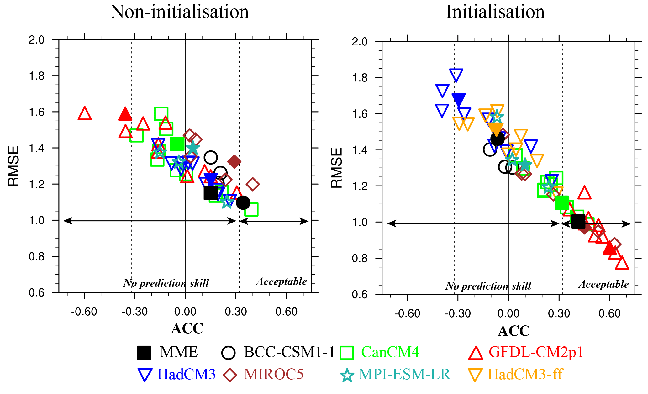
Figure 3 Performance of the model ensemble member (open marker) and its ensemble mean (solid marker) on the EASM index. The abscissa and ordinates are the anomaly correlation coefficient (ACC) and the root mean square error (RMSE), respectively. The observation of the EASM index is calculated by zonal wind at 850 hPa from the ERA-Interim reanalysis data. The black dotted lines indicate the significance level at 0.1. The vertical black line represents the correlation between the simulation and the observation of the EASM index at 0.

4 EASM–ENSO coupled mode in CMIP5

We employ the EOF method to analyse the anomaly in the leading EOF modes of the six meteorological variables in the EASM region (0^∘–50^∘ N, 100^∘–140^∘ E). The first EOF mode of the rainfall is characterised by a “sandwich” pattern, which shows sharp contrast between the prominent rainfall centre over Malaysia, the Yangtze River valley, and the south of Japan and the enhanced rainfall over the Indo-China peninsula and the Philippine Sea (Fig. 4). The increased precipitation is associated with cyclones in the low level (850 hPa) and anticyclones in the upper level (200 hPa).

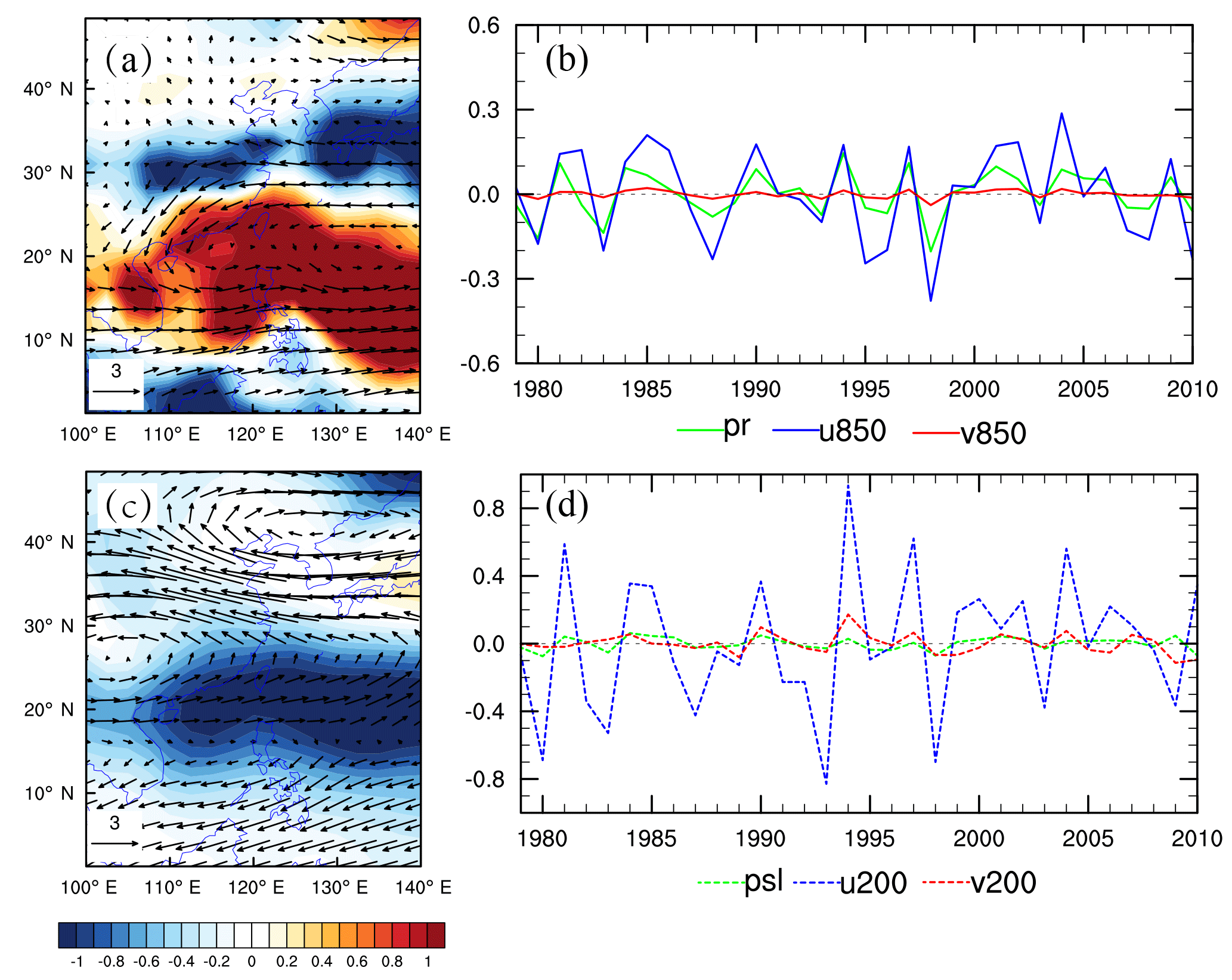
Figure 4 Spatial distribution of the first leading EOF mode of June–July–August precipitation and winds over 850 hPa (a), mean sea level pressure and winds over 200 hPa (c), and the associated principal component (PC; b, d). The GPCP and the ERA-Interim data from 1979–2005 are used for the EOF analysis in the EASM domain.

The correlation coefficient of the first eigenvector and the associated principal component (PC) between the model simulation and the observation in the non-initialised and the initialised simulation is presented in Fig. 5. Models capture the eigenvector of the first EOF for the six meteorological fields in the non-initialised simulation. However, they fail to reproduce the associated PC of the first leading EOF mode. Compared to the non-initialised simulation, models show no improvement in simulating the first leading EOF mode of rainfall, but exhibit a better performance in representing the first leading EOF mode of zonal wind. The CanCM4 and the GFDL-CM2p1 capture the first PC of ua850, but not the other five models. For the zonal wind at 200 hPa, the BCC-CSM1-1 fails to simulate its first EOF mode, while the other six models can. Only the GFDL-CM2p1 accurately simulates the first EOF eigenvectors and the associated PC of va850, which cannot be reproduced in the other models. No model captures the spatial–temporal variation in the first EOF mode of meridional wind at 200 hPa. In addition, the GFDL-CM2p1 and the MIROC5 simulate a reasonable leading EOF mode and associated PC of psl, while the other models do not capture it.

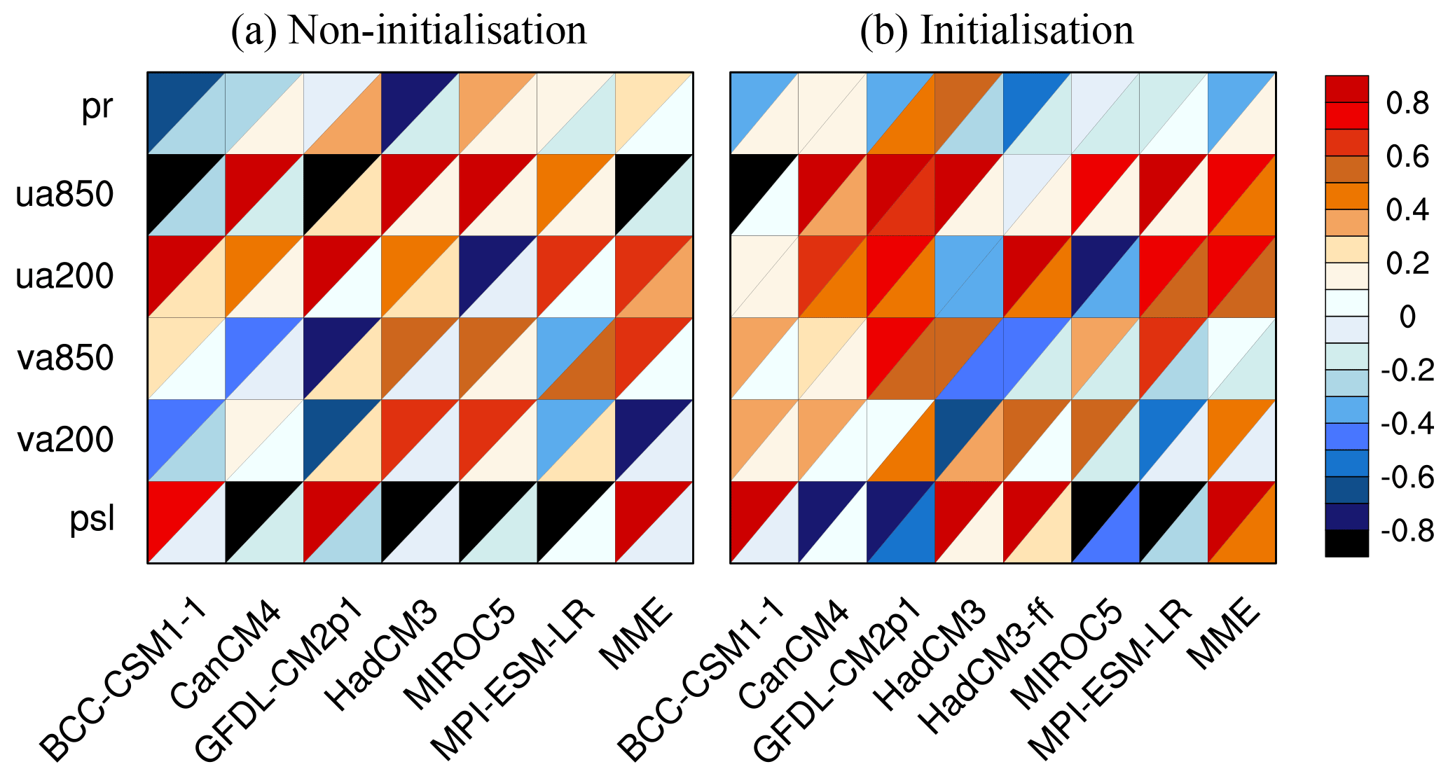
Figure 5 Portrait diagram display of correlation metrics between the observation and the model simulation of the first leading EOF mode for the six fields in the non-initialisation (a) and the initialisation (b). Each grid square is split by a diagonal in order to show the correlation with respect to both the eigenvector (upper left triangle) and its associated principal component (lower right triangle) reference datasets.

Figure 6 Fraction of variance (%) explained by the first EOF mode for six fields in the non-initialisation (a) and the initialisation (b).

Figure 6 shows the fractional (percentage) variances of the six variables from the first EOF mode with the total variances from the observation and the model simulation with (without) initialisation. The observational total variances for the pr, the ua850, the ua200, the va850, the va200, and the psl are depicted by the first leading EOF mode in 21.2, 59.0, 36.5, 20.6, 28.5, and 50.0 percent, respectively. The prediction systems simulate a comparable explanatory variance, which shows a slight discrepancy for the first leading mode in the non-initialisation. From the non-initialised to initialised simulation, the prediction systems tend to enhance the first EOF leading mode because they show larger fractional variances of the total variances of six variables. We note that the CanCM4 and the GFDL-CM2p1 significantly increase the fractional variances from non-initialisation to initialisation.

Figure 7 Model prediction skill of Niño3.4 (red) and SOI (blue) from DJF to SON in non-initialised (a) and initialised (b) simulations. Green diagrams show the correlation coefficient between the model simulation of Niño3.4 and the SOI. Box and whisker diagrams show the ensemble mean of each model (asterisk), median (horizontal line), 25th and 75th percentiles (box), and minimum and maximum (whisker). The two black dotted lines indicate the 0.05 significance level based upon a Student's t test.

The ENSO is the dominant mode of inter-annual variability in the coupled ocean and atmosphere climate system, which has strong effects on the inter-annual variation of the EASM (Wang et al., 2000; Wu et al., 2003). Wang et al. (2015) concluded that the first EOF leading mode of the ASM is the ENSO developing mode. As previously mentioned, the first EOF mode is improved in the initialised simulations compared to the non-initialised simulation. This also can be found in the ENSO indices (Fig. 7). The individual members and their ensemble mean of the six models show a low correlation coefficient to observational Niño3.4 and the SOI in the non-initialised simulations. The two indices show strong anti-phases in the observation, with the correlation range being −0.94 to −0.92 for four seasons (DJF, MAM, JJA, SON). Without initialisation, the models can describe the anti-correlation between Niño3.4 and the SOI, but with a weaker correlation. Compared to the non-initialisation, there is a significant improvement for models in capturing the observation of Niño3.4 and the SOI in the initialised experiments. The initialisation lowers the spread of Niño3.4 and the SOI in all six models. There is a noticeable change between the model in producing the relationship between Niño3.4 and the SOI. We find that the GFDL-CM2p1 (HadCM3) shows a lower (higher) Niño3.4–SOI correlation in the initialised than in the non-initialised simulations. With initialisation, the ensemble mean of each model outperforms its individual members in capturing Niño3.4 and the SOI, while without initialisation it shows a worse performance than that of the individual members in simulating Niño3.4 and the SOI.

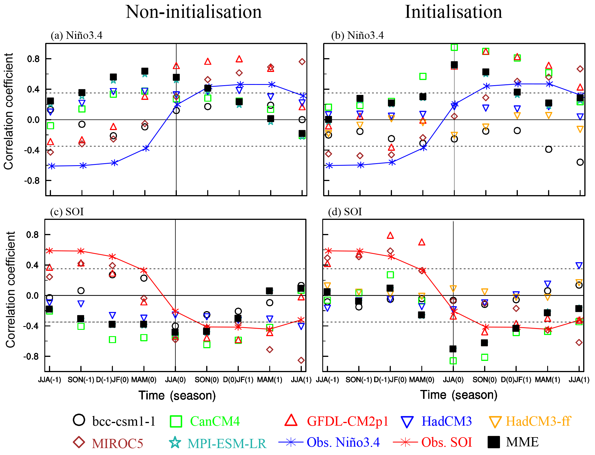
Figure 8 Lead–lag correlation coefficients between the EASM index and Niño3.4 (a), as well as SOI (c) in non-initialised simulations (a,c) and initialised ones (b, d) for observation (marker line) and models (marker) from JJA(−1) to JJA(+1). The two black dotted lines are the 0.05 significance level based upon a Student's t test. The vertical line represents JJA(0), where the simultaneous correlations between the EASM index and Niño3.4, as well as SOI are shown.

The EASM strongly relies on the preseason ENSO signal due to the lag response of the atmosphere to the SST anomaly (Wu et al., 2003). The lead–lag correlation coefficients between the EASM index and Niño3.4, as well as the SOI from JJA(−1) to JJA(+1) are illustrated in Fig. 8. The preseason Niño3.4 (SOI) presents a significant negative (positive) correlation with the EASM, while the postseason Niño3.4 (SOI) shows a notable positive (negative) correlation. This lead–lag correlation coefficient phase is called the Niño3.4 SOI–EASM coupled mode (Wang et al., 2008b). In the non-initialised cases, the models do not produce the teleconnection between the ENSO and the EASM. The CanCM4, the HadCM3, and the MPI-ESM-LR fail to represent the lead–lag correlation coefficient differences between preseason and postseason ENSO and EASM. The BCC-CSM1-1, the GFDL-CM2p1, and the MIROC5 capture the coupled mode of the ENSO and the EASM. However, the preseason ENSO has a weak effect on the EASM. Compared to the non-initialised cases, the MIROC5 and the GFDL-CM2p1 both demonstrate a significant improvement in simulating Niño3.4 SOI–EASM coupled mode in the initialisation. The BCC-CSM1-1, the HadCM3, and the HadCM3-ff show no improvement, with insignificant correlation between Niño3.4 (SOI) and the EASM. The CanCM4 and the MPI-ESM-LR indicate a higher correlation between the EASM and the simultaneous to postseason ENSO than to the preseason ENSO.

5 Discussion

The model exhibits a better performance in simulating the general circulation of the EASM with initialisation. Thus, initialisation is helpful in forecasting the EASM on a seasonal timescale. There are two initialisation methods in our study: full-field initialisation and anomaly initialisation (Table 1). The full-field initialisation produces more skilful predictions on the seasonal timescale in predicting regional temperature and precipitation (Magnusson et al., 2013; Smith et al., 2013). Nevertheless, for predicting the EASM, there is no significant difference between the two methods. We can see that both the GFDL-CM2p1 and the MIROC5 have significant improvement in capturing the EASM with full-field and anomaly initialisation, respectively. Only the HadCM3 is initialised by the two initialisation techniques. However, both of these initialised techniques produce poor predictions of the EASM with no major differences.

The current initialisation strategy updates the observed atmospheric component (i.e. zonal and meridional wind, geopotential height, etc.) and the SST (Meehl et al., 2009, 2014; Taylor et al., 2012). With initialisation, the SST conveys its information via the large heat content of the ocean to the coupled system. Therefore, an index indicating an ocean oscillation like Niño3.4 shows seasonal-to-decadal prediction skill (Jin et al., 2008; Luo et al., 2008; Choi et al., 2016). The models studied here demonstrate a prediction skill in simulating Niño3.4 and the SOI due to this effect. The change in the correlation between Niño3.4 and the SOI is insignificant from non-initialised to initialised simulations. We therefore conclude that the relationship between Niño3.4 and the SOI depends more on the model parameterisation than on the initial condition.

Wang et al. (2015) found that the second EOF mode of ASM is the Indo-western Pacific monsoon–ocean coupled mode, the third is the Indian Ocean dipole (IOD) mode, and the fourth is the trend mode. The Indo-western Pacific monsoon–ocean coupled mode is the atmosphere–ocean interaction mode (Wang et al., 2013; Xiang et al., 2013), which is supported by a positive thermodynamic feedback between the western North Pacific (WNP) anticyclone and the underlying Indo-Pacific sea surface temperature anomaly dipole over the warm pool (Wang et al., 2015). The IOD increases precipitation from the South Asian subcontinent to south-eastern China and suppresses precipitation over the WNP (Wang et al., 2015). It affects the Asian monsoon by the meridional asymmetry of the monsoonal easterly shear during boreal summer, which can particularly strengthen the northern branch of the Rossby wave response to the south-eastern Indian Ocean SST cooling, leading to an intensified monsoon flow and an intensified convection (Wang and Xie, 1996; Wang et al., 2003, 2015; Xiang et al., 2011). We note that the models simulate a reasonable first EOF mode, but illustrate no skill in capturing the other EOF leading modes (not shown). We argue that the models cannot represent the monsoon–ocean interaction well, even with initialisation. The models do not simulate the third EOF leading mode of the EASM since the predictability of the IOD extends only over a 3-month timescale (Choudhury et al., 2015). The current initialisation strategies (both anomaly and full field) enhance the ENSO signal in the model simulations with a higher explained fraction of variance. Kim et al. (2012) described a similar finding in ECMWF system 4 and NCEP Climate Forecast System version 2 (CFSv2) seasonal prediction simulations. With initialisation, the models predict ENSO on a seasonal timescale well, which leads to an overly strong modulation of the EASM by ENSO (Jin et al., 2008; Kim et al., 2012).

It is worth mentioning that it was an extremely weak monsoon and strong El Niño year in 1998. The CanCM4, the GFDL-CM2p1, the MIROC5, and the MPI-ESM-LR have the ability to simulate the extreme monsoon event, while the BCC-CSM1-1 and the HadCM3 do not capture it even with initialisation. There is potential for the BCC-CSM and the HadCM to improve the teleconnection between the ENSO and the EASM.

This study discusses six CMIP5 models in predicting the EASM on a seasonal timescale. The six models are earth system coupled models which present a better SST–monsoon teleconnection than CMIP3 models (Sperber et al., 2013) and IRI (International Research Institute for Climate and Society) models (Barnston et al., 2010). There are four AGCMs contributing to the IRI prediction system, including ECHAM4.5, CCM3.6, COLA, and GFDL-AM2p14. These models are forced to forecast the climate on a seasonal timescale with prescribed SST. Barnston et al. (2010) found that the models showed low prediction skill over East Asia. Therefore, the IRI prediction system cannot be used to predict the EASM. There are two seasonal forecast application systems, the ECMWF system and the NCEP CFS. Both the application systems have low prediction skill of EASM (Kim et al., 2012; Jiang et al., 2013). The CMIP5 models have potential to be developed as an application system for EASM seasonal prediction, especially the GFDL-CM2p1 and the MIROC5.

To better predict the short- to long-term climate, the World Climate Research Programme (WCRP) launched two new projects: the Climate-system Historical Forecast Project (CHFP; Kirtman and Pirani, 2009; Tompkins et al., 2017) and the Subseasonal-to-Seasonal (S2S) Prediction Project (Vitart et al., 2017). The two projects coordinate most climate modelling research groups and provide a large range of forecast datasets. A comprehensive comparison of all the CHFP and S2S data with the CMIP5 simulations regarding the seasonal prediction skill of the EASM is certainly an interesting topic, which should be addressed in an additional paper.

We have compared six CMIP5 systems with their respective initialisation strategies. The GFDL-CM2p1 and the MIROC5 have the potential to serve as a seasonal forecast application system even with their current initialisation method. These models have great potential to optimise the SST–EASM interaction simulation performance to improve their seasonal prediction skill of the EASM.

6 Summary

Six earth system models from CMIP5 have been selected in this study. We have analysed the improvement of rainfall, mean sea level pressure, zonal wind, and meridional wind in the EASM region from non-initialisation to initialisation. The low prediction skill of summer monsoon precipitation is due to the uncertainties of cloud physics and cumulus parameterisations in the models (Lee et al., 2010; Seo et al., 2015). The models show a better performance in capturing the inter-annual variability of zonal wind than precipitation with initialisation. Thus, the zonal wind index is an additional factor which can indicate the prediction skill of the model. When we calculate the WF index in both non-initialised and initialised simulations, the GFDL-CM2p1 and the MIROC5 show a significant advancement in simulating the EASM from the non-initialised to initialised simulation with a lower RMSE and a higher ACC. There is a slight change in the WF index calculated from the BCC-CSM1-1, the CanCM4, and the MPI-ESM-LR data with initialisation. Compared to the non-initialised simulation, the HadCM3 loses prediction skill, especially with anomaly initialisation.

To test the possible mechanisms of the models' performance in non-initialisation and initialisation, we have calculated the leading mode of the six fields associated with the EASM. The models demonstrate a better agreement with the observational first EOF mode in the initialised simulations. The first leading mode of zonal wind at 200 hPa shows a significant improvement in the models except the BCC-CSM1-1 with initialisation. Therefore, a potential predictor might be an index based upon the zonal wind at 200 hPa. Compared to non-initialisation, the models enhance the first EOF mode with a higher fraction of variance to the total variance after initialisation. The first EOF mode of the EASM is the ENSO developing mode (Wang et al., 2015). We have analysed the seasonal simulating skill of Niño3.4 and the SOI in each model. The models show a poor performance in representing Niño3.4 and the SOI in the non-initialised simulation. Initialisation improves the model simulating skill of Niño3.4 and the SOI. The initialised simulations decrease the spread of ensemble members in the models. We find that there is no significant change in the models reproducing the correlation between Niño3.4 and the SOI from non-initialisation to initialisation.

In general, the preseason warm phase of the ENSO (El Niño) leads to a weak EASM producing more rainfall over the South China Sea and north-west China and less rainfall over the Yangtze River valley and southern Japan; the cold phase of the ENSO (La Niña) illustrated a reverse rainfall pattern to El Niño in East Asia. The preseason Niño3.4 (SOI) exhibits a strong negative (positive) correlation with the EASM, while the correlation between the postseason Niño3.4 (SOI) and the EASM illustrated an anti-phase from the preseason. In the non-initialised simulations, the models do not capture the Niño3.4 SOI–EASM coupled mode. The MIROC5 is the only model that has the ability to represent the Niño3.4–EASM coupled mode with initialisation. For the SOI–EASM coupled mode, the GFDL-CM2p1 and the MIROC5 capture it in the initialisation, while the BCC-CSM1-1, the HadCM3, the HadCM2-ff, the CanCM4, and the MPI-ESM-LR do not. Therefore, we argue that the differential depiction of the ENSO–EASM coupled mode in CMIP5 models leads to their differential responses to initialisation.