Assessing the performance of LPJmL-5 in simulating vegetation responses to normal and multi-year droughts

Climate change is expected to increase the frequency and severity of Multi-Year Droughts (MYDs), but their impacts on vegetation remain poorly understood. While satellite records offer valuable insights, they only cover recent decades, limiting the number of MYDs available for analysis. The dynamic global vegetation model LPJmL-5 can simulate vegetation dynamics under varying climate conditions and over longer temporal scales than are typically available from satellite observations. However, its ability to capture vegetation responses to drought, including MYDs, has not yet been systematically evaluated against observation-based datasets. In this study, we benchmark LPJmL-5 against MODIS-derived gross primary production (GPP) to assess how well the model reproduces vegetation responses to drought. We find that LPJmL-5 captures the key temporal and spatial dynamics of drought-related GPP observed by MODIS, although notable differences remain. In particular, LPJmL-5 tends to overestimate vegetation response at the onset of MYDs and shows some rapid recovery behaviour, resulting in muted overall drought impacts. Vegetation responses also vary by type: drought dynamics in croplands are captured relatively well, whereas responses in boreal and temperate vegetation are underestimated in magnitude. These discrepancies appear to be linked to simplified model representations of vegetation stress and mortality, which limit long-term vegetation loss. Beyond drought conditions, LPJmL-5 reproduces absolute GPP values reasonably well in some regions, but performance declines in parts of the Southern Hemisphere and in cropland-dominated areas. This suggests that general GPP simulation performance is not necessarily linked to performance during drought conditions. Overall, this benchmarking highlights strengths and limitations in how LPJmL-5 represents vegetation responses to drought and provides a foundation for future studies of vegetation responses to multi-year droughts.

1 Introduction

Multi-Year Droughts (MYDs) can have severe impacts on natural vegetation and croplands, ranging from reduced vegetation health to diminished ecosystem resilience and increased tree mortality (Choat et al., 2018; DeSoto et al., 2020; Gessler et al., 2020; Allen et al., 2010; Cooley et al., 2015; Dong et al., 2019; Moravec et al., 2021; Jiao et al., 2020; Wittwer and Waschik, 2021; Hughes et al., 2019). Although less frequent than shorter droughts, MYDs have already been observed worldwide (van Mourik et al., 2025) and are projected to increase in both frequency and severity (van der Wiel et al., 2023). Understanding how vegetation responds to MYDs is therefore essential for assessing ecosystem vulnerability and anticipating future changes in vegetation health and productivity.

Satellite remote sensing datasets, such as those derived from MODIS, have been widely used to monitor vegetation dynamics and assess drought impacts (Ruijsch et al., 2025; van Hateren et al., 2021; Dong et al., 2019; Yang et al., 2021). These datasets offer global coverage with high spatial and temporal resolution, making them valuable tools for analysing vegetation responses during droughts. These remotely sensed observations show that, while MYDs generally reduce vegetation productivity and increase stress, the magnitude and direction of these impacts vary across regions. Local water and energy availability can influence responses, resulting in weak, neutral, or even positive effects in some cases (Ruijsch et al., 2025; van Hateren et al., 2021; Dong et al., 2019; Yang et al., 2021). However, satellite records typically extend back only to around 2000 (Didan, 2015a, b), limiting the number of MYDs available for analysis and reducing the statistical robustness of drought impact assessments based solely on remote sensing datasets.

Dynamic Global Vegetation Models (DGVMs), such as LPJmL-5 (von Bloh et al., 2018), can simulate vegetation dynamics under varying climate conditions and over longer temporal scales than are typically available from satellite observations. LPJmL-5 has been widely used to study vegetation and agricultural dynamics under historical and projected climate scenarios (von Bloh et al., 2018; Müller and Robertson, 2014; Gerten et al., 2013), and its performance has been extensively evaluated (Schaphoff et al., 2018b, a; von Bloh et al., 2018). However, while the model performs well in many aspects, its ability to capture vegetation responses to (multi-year) droughts has not yet been systematically evaluated against observation-based datasets.

In this study, we benchmark LPJmL-5 against MODIS-derived GPP to evaluate how well the model reproduces vegetation responses to both MYDs and normal droughts (NDs; droughts lasting less than one year). Specifically, we assess the model's ability to capture the magnitude, timing, and spatial patterns of drought-induced GPP anomalies across different regions and vegetation types. This evaluation provides insight into observed drought response behaviour and highlights where LPJmL-5 realistically represents drought stress and recovery, as well as where improvements are needed.

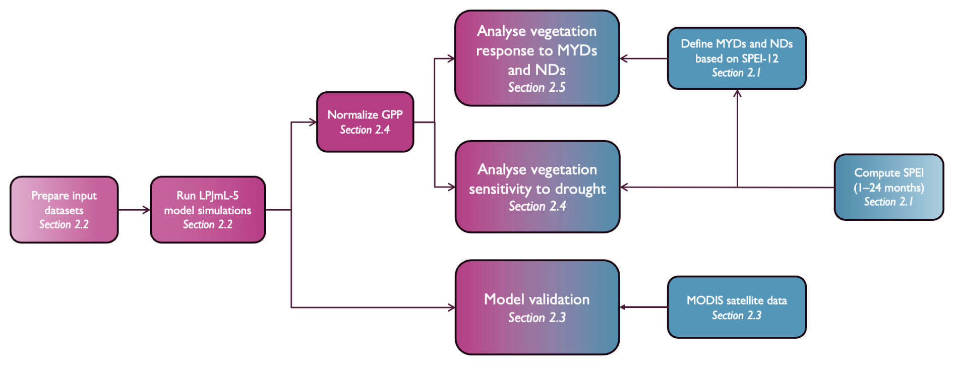
Figure 1 Schematic overview of the methodological workflow used in this study. The processes include drought classification, LPJmL-5 model simulations, comparison with MODIS-derived GPP, and the analysis of vegetation responses to both MYDs and NDs across selected focus regions. Blue elements represent observational data, while pink elements indicate model outputs.

2 Materials and methods

This section outlines the definitions, vegetation model, data, and methods used to evaluate vegetation responses to (multi-year) droughts (Fig. 1). Section 2.1 defines MYDs and NDs, Sect. 2.2 describes the LPJmL-5 model, followed by model validation against observational data in Sect. 2.3. Section 2.4 and 2.5 explain how vegetation responses to (multi-year) droughts are defined. Finally, Sect. 2.6 introduces the focus regions analysed in this study.

2.1 Drought identification

Drought indices are essential for studying drought events, as they allow for consistent comparison of drought characteristics across space and time. In this study, we used the Standardized Precipitation Evapotranspiration Index (SPEI), which accounts for both water supply (precipitation, P) and atmospheric water demand (potential evapotranspiration, PET) (Vicente-Serrano et al., 2010). SPEI is particularly suitable for assessing drought impacts on vegetation as vegetation is not only impacted by lack of water supply via P, but also the increase in atmospheric water demand via PET.

SPEI was computed at multiple timescales (1–24 months) using P and PET derived from W5E5 reanalysis data (see Table 1, Lange et al., 2022). Both P and PET were aggregated to monthly values to generate monthly SPEI outputs. A detailed description of the SPEI calculation is provided in Sect. S1 in the Supplement.

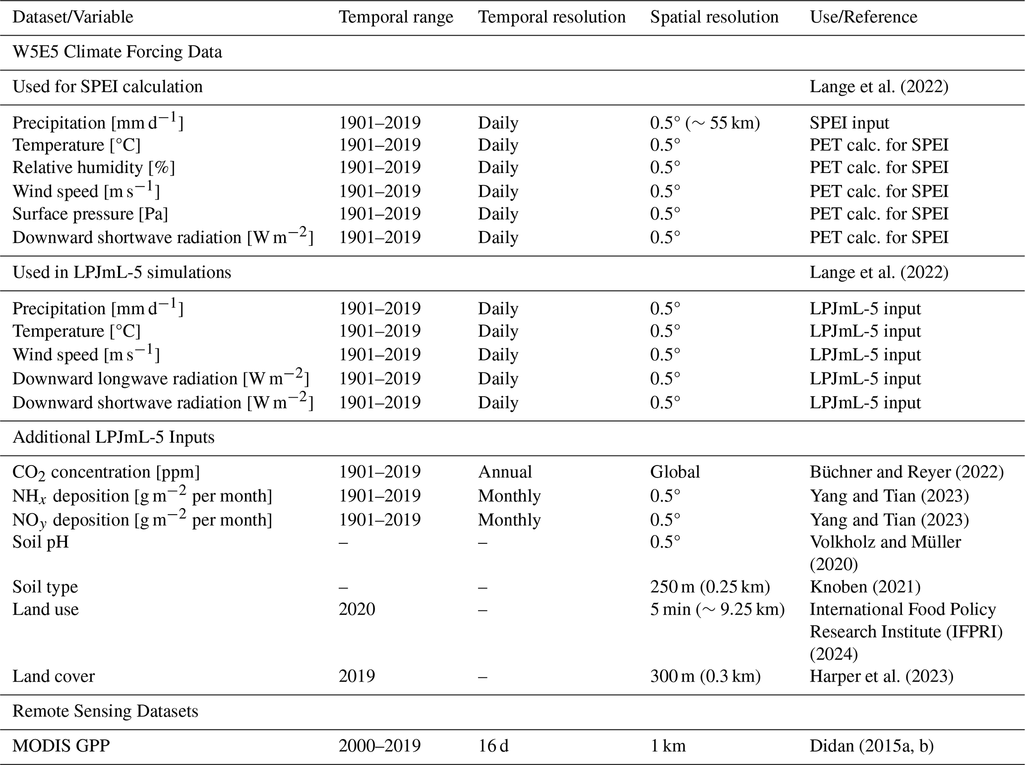
Lange et al. (2022)Lange et al. (2022)Büchner and Reyer (2022)Yang and Tian (2023)Yang and Tian (2023)Volkholz and Müller (2020)Knoben (2021)International Food Policy Research Institute (IFPRI) (2024)Harper et al. (2023)Didan (2015a, b)

Table 1 Overview of datasets and variables used in this study. W5E5 climate variables are grouped by their application in either SPEI calculation or LPJmL-5 simulations.

To define MYDs and NDs, we focused on SPEI calculated at a 12-month timescale (SPEI-12), as it captures multi-year drought conditions while minimizing seasonal variability. Following Wiel et al. (2022), MYDs are defined as periods where SPEI-12 remains below −1 for at least 12 consecutive months. The threshold of −1 was chosen to represent moderate to extreme droughts (McKee et al., 1993). While the start date of the drought is only identified as the first month where SPEI-12 dips below −1, this definition already takes into account the accumulated P and PET over the 12 months leading up to the start of the drought. Ruijsch et al. (2025) evaluated the impact of different SPEI aggregation periods and concluded that the SPEI-12 is suitable for capturing multi-year drought dynamics.

To distinguish MYDs from shorter drought events, we define NDs as periods where SPEI-12 remains below −1 for less than 12 consecutive months. This definition ensures that each drought event is consistently categorized as either an MYD or ND, allowing us to systematically compare their respective impacts on vegetation.

2.2 Dynamic global vegetation modelling using LPJmL-5

In this study, the DGVM LPJmL-5 (v5.7.9, von Bloh et al., 2018) was used to simulate vegetation responses to MYDs. LPJmL-5 builds on LPJmL-4 and simulates both natural and agricultural vegetation, linking their growth and productivity through consistent water, carbon, and energy fluxes (Schaphoff et al., 2018b). LPJmL-5 makes use of the big-leaf representation for different Plant Functional Types (PFTs) that can coexist within a grid cell and compete for resources such as light, water, and nitrogen (von Bloh et al., 2018). Land cover can either be simulated dynamically or be prescribed, both of which are used in this study. In contrast, Crop Functional Types (CFTs) are always prescribed, with a distinction between irrigated and rainfed crops. Each grid cell can contain both managed and natural vegetation fractions, allowing for a realistic subgrid representation of land-use. CFTs only appear when crops are sown and grow on soil areas separate from natural vegetation (von Bloh et al., 2018). The model also includes key physiological processes such as photosynthesis, gross primary production, evapotranspiration, and plant responses to soil moisture and drought stress (Schaphoff et al., 2018b). The terrestrial nitrogen cycle is incorporated to account for nutrient limitations to plant growth (von Bloh et al., 2018). This makes that LPJmL-5 contains all the necessary processes to study vegetation responses to drought, though its performance may still vary across regions and vegetation types.

2.2.1 Drought in the LPJmL-5 model

In LPJmL-5, GPP is first calculated as a potential GPP, based on the light-limited (JE) and Rubisco-limited (JC) rates and on the absorbed photosynthetically active radiation (APAR; Schaphoff et al., 2018b). This potential GPP is then constrained by soil water availability. When the water supply cannot meet atmospheric demand, water stress develops and the potential GPP is reduced to the actual GPP.

Drought can further influence GPP through phenology. LPJmL-5 includes a phenology function that controls how active the canopy is, ranging from 0 (no active canopy) to 1 (fully active canopy). When phenology declines, leaf area and FAPAR decrease, thereby reducing GPP. The phenology is determined by four limiting functions: cold temperature, light availability, water availability, and heat stress (Schaphoff et al., 2018b). Each factor varies between 0 (full limitation) and 1 (no limitation), and their combined effect defines the total phenology. The limiting functions follow logistic curves and include a memory term, meaning that canopy responses are delayed and differ across PFTs (Schaphoff et al., 2018b). The associated parameters were calibrated by fitting simulated FAPAR to satellite-derived FAPAR over 30 years (Schaphoff et al., 2018b).

Vegetation in LPJmL-5 is represented using the big-leaf representation, meaning that all leaves of a PFT within a grid cell are treated as a single canopy layer with an average temperature, photosynthesis, and water use. Under drought, reductions in phenology and water supply therefore shrink this “big leaf” and makes it less productive, rather than simulating individual trees.

Finally, LPJmL-5 does not simulate explicit drought-induced mortality. Instead, mortality emerges indirectly from low productivity and heat stress, and is capped by a maximum annual mortality rate (Schaphoff et al., 2018b). As a result, prolonged water deficits only lead to die-off when plants repeatedly fail to maintain sufficient biomass. Moreover, this mortality process is only active when land cover is simulated dynamically and is not applied when land cover is prescribed.

2.2.2 LPJmL-5 input and output

In this study, LPJmL-5 was used to simulate vegetation dynamics at a 0.1° spatial resolution (∼11 km) and a daily temporal resolution. The model was forced with meteorological forcing, soil properties, land use, and land cover derived from observational datasets (Table 1). Daily meteorological forcings are taken from the W5E5 dataset and include temperature, precipitation, downward longwave and shortwave radiation, and wind speed (Lange et al., 2022). Soil inputs include static variables such as soil pH (Volkholz and Müller, 2020) and soil type (Knoben, 2021), as well as dynamic inputs like monthly nitrogen deposition (NH₄ and NO₃) (Yang and Tian, 2023). Annual atmospheric CO₂ concentrations were taken from Büchner and Reyer (2022). Land use and country code data are provided at a 5 min (∼9.25 km) spatial resolution, and soil type data at 250 m. All three were regridded to a 0.1° spatial resolution, whereas soil pH and climate forcing data are downscaled using a nearest neighbour interpolation from their original 0.5° (∼55 km) resolution.

The land use map was primarily derived from International Food Policy Research Institute (IFPRI) (2024), which provides information on crop areas. However, the crop types in this dataset did not directly match the CFTs used in LPJmL-5, so they were reclassified accordingly. Additionally, pasture areas are a land-use type in LPJmL-5 but were not included in the IFPRI dataset. These were obtained from the ESA land cover maps (Harper et al., 2023) and incorporated into the land-use input. For the land cover input, we used the ESA PFT maps (Harper et al., 2023), which provide fractional cover of tree, shrub, and grass types. Because LPJmL-5 separates PFTs by climate zone (tropical, temperate, and boreal), we reclassified the ESA PFT maps to match the PFTs in LPJmL-5 using the Köppen-Geiger classification (Beck et al., 2023), following the approach of Forkel et al. (2019) (see Sect. S6). Shrubs were merged with the corresponding tree PFTs because LPJmL-5 does not distinguish between these growth forms. This procedure ensured that land-use and land-cover inputs were compatible with the vegetation types represented in LPJmL-5.

LPJmL-5 provides a multitude of vegetation-related outputs on ecological, hydrological, and agricultural components (such as leaf area index, soil moisture, runoff, and crop yields). To study vegetation response to drought, this study used the monthly Gross Primary Production (GPP), which is the amount of carbon captured from the atmosphere through vegetation photosynthesis (Beer et al., 2010). The GPP output used in this study was produced at a 0.1° spatial and monthly temporal resolution.

2.3 Model validation

2.3.1 MODIS GPP as validation dataset

In this study, we evaluated simulated GPP by LPJmL5 against MODIS satellite derived GPP estimates. Although MODIS GPP is widely used, it is not purely observational, but derived using the MOD17 light-use efficiency algorithm and relies on inputs such as MODIS FPAR, meteorological drivers, and land-cover classification (Running and Zhao, 2021). Therefore, before using it as a validation dataset, we assessed how well the MODIS GPP product represents vegetation productivity (Sect. S3).

We compared MODIS GPP with two satellite products that are more directly observation-based: the Enhanced Vegetation Index (EVI; Didan, 2015a, b) and solar-induced fluorescence (SIF; Wang and Zhang, 2023). Both comparisons showed strong and statistically significant relationships, particularly outside tropical regions, indicating that MODIS GPP captures large-scale variability in vegetation productivity. Other validation studies report similar limitations, with reduced performance mainly in tropical ecosystems. A full description of these analyses is provided in Sect. S3. Together, these results support the use of MODIS GPP as a validation product for LPJmL5, while acknowledging that uncertainties are larger in tropical regions.

To ensure consistency with LPJmL5 output, the MODIS GPP data was regridded to a spatial resolution of 0.1° and a monthly temporal resolution. Because LPJmL-5 provides a single GPP value per grid cell, each cell was assigned to its dominant vegetation type. CFT fractions were aggregated into one cropland category, while natural PFTs were grouped into broader classes: tropical trees, temperate trees, boreal trees, tropical C₄ grass, temperate C₃ grass, and polar C₃ grass (Appendix A).

2.3.2 Kling-Gupta Efficiency

To quantify model performance, we used the Kling-Gupta Efficiency (Gupta et al., 2009), which combines correlation, bias, and variability into a single metric:

$$\begin{array}{}\text{(1)}& \text{KGE}=\mathrm{1}-\sqrt{(r-\mathrm{1}{)}^{\mathrm{2}}+(\mathit{\alpha }-\mathrm{1}{)}^{\mathrm{2}}+(\mathit{\beta }-\mathrm{1}{)}^{\mathrm{2}}},\end{array}$$

where r is the linear correlation between observations and simulations, $\mathit{\alpha }=\frac{{\mathit{\sigma }}_{\mathrm{sim}}}{{\mathit{\sigma }}_{\mathrm{obs}}}$ a measure of the variability error, and $\mathit{\beta }=\frac{{\mathit{\mu }}_{\mathrm{sim}}}{{\mathit{\mu }}_{\mathrm{obs}}}$ a bias term. Here, σ_obs and σ_sim are the standard deviations of the observations and simulations, respectively, while μ_sim and μ_obs are the corresponding means. KGE values greater than −0.41 indicate that the model performs better than the mean benchmark, while a value of 1 indicates perfect agreement between simulations and observations (Knoben et al., 2019). This allows us to assess how well LPJmL-5 simulates GPP for different PFTs compared to MODIS, and to identify structural patterns in performance across the globe.

2.4 Vegetation sensitivity to varying drought timescales

After evaluating how well LPJmL-5 simulates general patterns of GPP compared to MODIS GPP, we examined how well LPJmL-5 can model vegetation responses to drought. Here, we aim to understand modelled vegetation sensitivity to drought without differentiating between “normal” and “multi-year” droughts. To ensure a fair comparison of vegetation responses across regions and to remove seasonal variation, the GPP data was normalized and standardized using z-score normalization resulting in a standardized GPP anomaly (GPP_SA). The reference normalization period was chosen to match the MODIS dataset (2000–2019) to avoid errors resulting from GPP trend differences between modelled and observed data.

Vegetation can respond differently to drought events of different durations. To capture this, we used the extreme-based method developed by Deng et al. (2022). This method examines how different drought durations affect vegetation across various SPEI timescales (ranging from 1 to 24 months). Specifically, we calculated the average GPP_SA response for each timescale and identified which one has the strongest negative impact during drought periods. This timescale is referred to as the dominant drought timescale and reflects how quickly vegetation responds to drought stress. Shorter timescales indicate faster, more sensitive responses, while longer timescales suggest a slower response and less drought-sensitive vegetation. For this analysis, a SPEI threshold of −1 was chosen to define atmospheric drought conditions, as suggested by McKee et al. (1993).

2.5 Vegetation response to MYDs

After determining how sensitive vegetation is to drought at different timescales, we further investigated how vegetation in LPJmL-5 responds to MYDs specifically. We compared MODIS observations and LPJmL-5 simulations by analysing global spatial patterns together with temporal dynamics in selected focus regions. Vegetation responses during MYDs were quantified by using the mean GPP_SA during MYD events.

2.6 Selection of focus regions

While this study primarily examines global drought patterns, it also focuses on selected focus regions to better understand local drought dynamics and how regional differences affect vegetation responses. The focus regions used in this study are: California (CAL), the Rhine-Meuse delta in western Europe (WEU), the Brahmaputra River basin spanning Bangladesh, India, Bhutan, and China (BRA), central Argentina (ARG), the Orange River basin in southern Africa (SA), and the Murray-Darling basin in Australia (AUS) (Appendix B). These regions correspond to the focus regions used by Ruijsch et al. (2025) examining MYD patterns. The focus regions were selected based on the number of MYDs that have occurred between 2000–2019, geographic and climatic diversity, and variation in vegetation types, ensuring a broad representation of both water- and energy-limited regions across different climate zones.

3 Results

The following sections describe different aspects of the analysis on the potential of LPJmL-5 to simulate vegetation response to (multi-year) droughts. Section 3.1 examines LPJmL's ability to reproduce satellite-derived GPP, while Sect. 3.2 and 3.3 focus on its ability to reproduce (multi-year) droughts.

3.1 General performance of LPJmL-5

To evaluate LPJmL-5's ability to simulate GPP, we compared modelled GPP to MODIS-derived GPP using two simulation setups: dynamic and prescribed land cover. The dynamic land cover setup allows vegetation fractions to shift in response to climate and includes background mortality, capturing potential vegetation loss (Schaphoff et al., 2018b). However, dynamic vegetation does not necessarily match observed vegetation types, which can lead to differences in GPP due to mismatched vegetation types. The prescribed land cover simulation maintains fixed vegetation fractions based on observed maps. This approach ensures that variations in GPP result from the model's ability to simulate vegetation productivity. However, this setup does not include background mortality, potentially causing an underestimation of vegetation loss. By comparing both setups, we can determine which one provides a better representation of satellite-derived GPP and choose the setup to be used in later analyses. Model performance is evaluated by comparing LPJmL-5 and MODIS GPP using the KGE metric (Sect. 3.1.1) and time series analysis (Sect. 3.1.2).

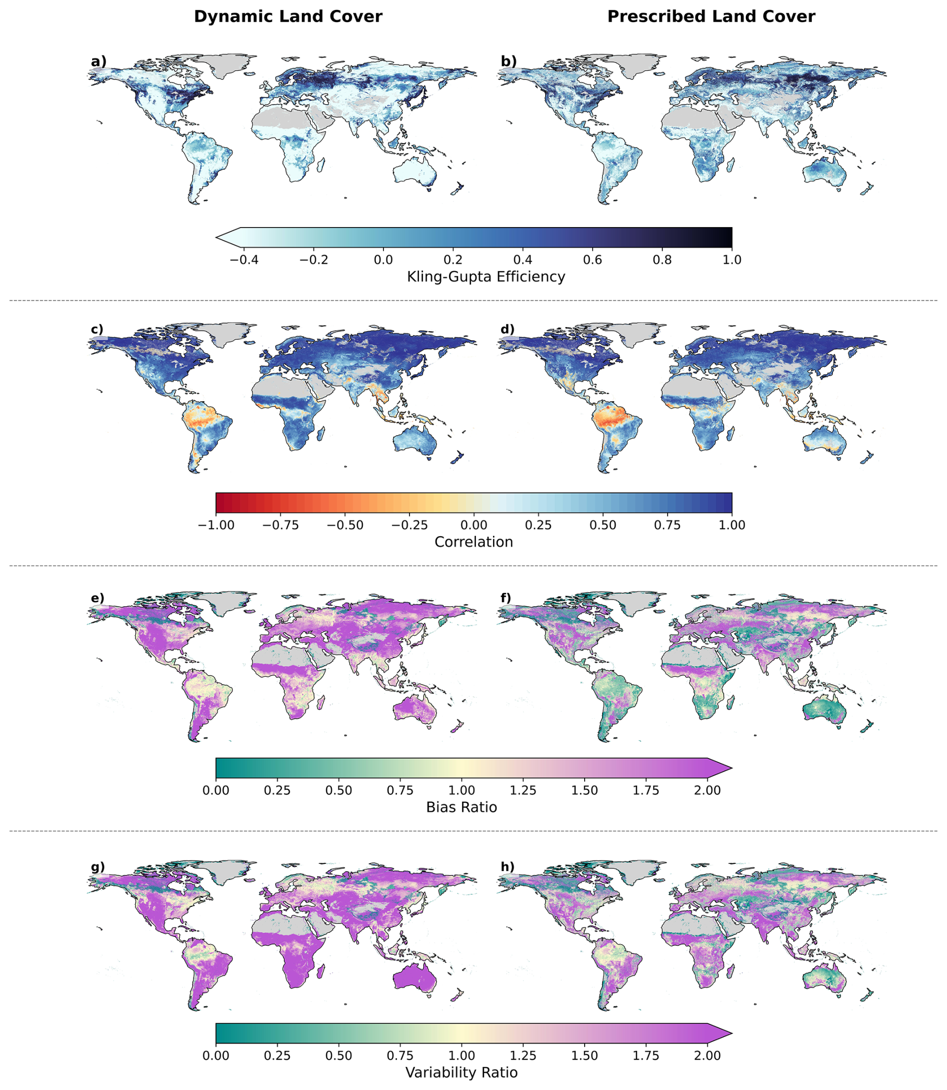
Figure 2 Spatial comparison of LPJmL-5 model performance using the Kling-Gupta Efficiency (KGE) metric and its components for dynamic (left column) and prescribed (right column) land cover simulations. The rows show (a–b) overall KGE, followed by its components: (c–d) correlation, (e–f) bias, and (g–h) variability.

3.1.1 Evaluating model performance with the KGE metric

Figure 2 shows the spatial distribution of the KGE and its components (correlation, bias, and variability) for both dynamic and prescribed land cover simulations. Overall, the prescribed land cover demonstrates a clear performance improvement over the dynamic simulation (Fig. 2a and b).

The dynamic land cover consistently shows low agreement with MODIS across all KGE components (Fig. 2c, e and g). The agreement is particularly poor in the Southern Hemisphere, with KGE values often falling below −0.41, which is the threshold for a skilful performance. In contrast, the Northern Hemisphere generally shows a better performance. Switching to prescribed land cover results in improved KGE scores globally. However, the performance difference between the Northern and Southern Hemispheres remains.

When examining the individual KGE components, the correlation between modelled and satellite-derived GPP is relatively high for both simulations, except in the tropical and semi-arid regions (Fig. 2c and d). This suggests that the intra-annual response to changing meteorological conditions is similar between LPJmL-5 and satellite-derived MODIS GPP.

Both the bias (Fig. 2e) and variability (Fig. 2g) components are overestimated in the dynamic land cover simulation. The bias frequently exceeds 2, except in the tropical regions, suggesting that the model's mean GPP is approximately double that of the satellite-derived value. The prescribed land cover simulation (Fig. 2f) significantly reduces this bias, particularly in tropical and temperate regions, bringing modelled GPP closer to the satellite-derived reference. A similar pattern is observed for the GPP variability, where the dynamic land cover shows overestimated variability (greater than 2) in Fig. 2g, while prescribed land cover reduces this variability (Fig. 2h).

These differences in model performance can be attributed to discrepancies between the modelled and observed vegetation types when using dynamic land cover. For example, we observe that LPJmL-5 simulates tree cover in regions where the ESA land cover map shows predominantly grasslands, such as Western Europe and parts of South Africa (see Appendix C and Sect. S5). These discrepancies in vegetation types lead to differences in GPP that are not related to the model's capability to simulate GPP responses to changing meteorological conditions, but rather to inconsistencies in vegetation cover. By using prescribed land cover fractions based on the ESA land cover map, we observe an improvement in model performance, with remaining errors linked to LPJmL-5's inability to accurately simulate the GPP response to changes in meteorological conditions.

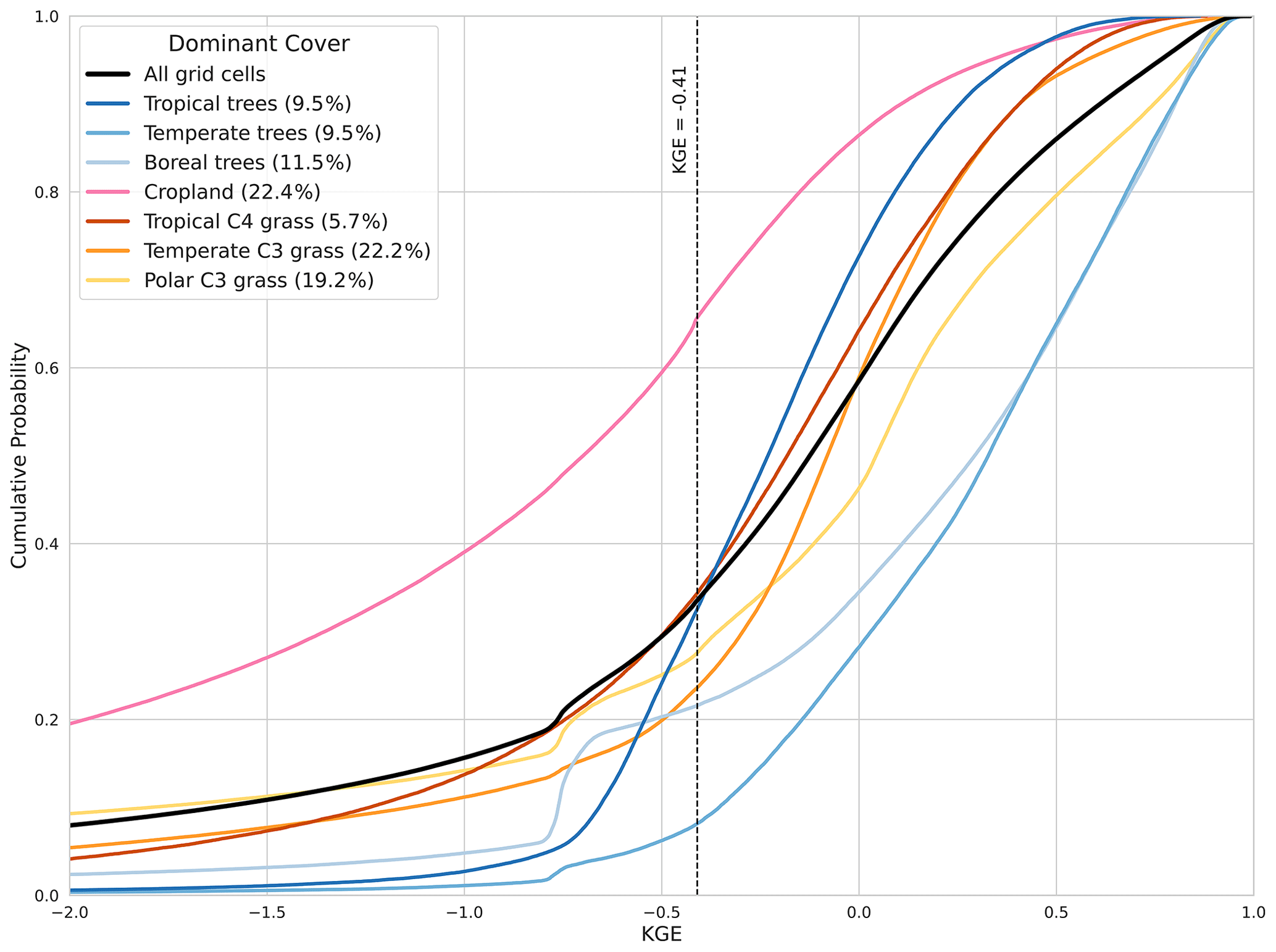
Figure 3 Cumulative distribution function (CDF) of the KGE of the prescribed land cover GPP for the different vegetation types in LPJmL-5. Percentages show the percentage of grid cells with that dominant land cover. Black dashed line indicates KGE $=-\mathrm{0.41}$. Values greater than −0.41 indicate that the model improved upon the mean benchmark.

To further assess model performance in the prescribed land cover simulation, we analyse the KGE distribution for each PFT, as shown in Fig. 3. This cumulative distribution function (CDF) displays the proportion of grid cells for each dominant vegetation type (Appendix A) that exceed the KGE threshold of −0.41, which represents the mean benchmark (Knoben et al., 2019).

The performance of LPJmL-5 varies significantly across PFTs. Croplands show the lowest agreement with satellite-derived GPP, with over 60 % of grid cells falling below the KGE $=-\mathrm{0.41}$ line. In contrast, temperate trees show the best agreement, with 90 % showing skilful GPP simulations. Approximately 80 % of areas dominated by boreal trees show good agreement with MODIS data. Polar and temperate C₃ grasses are the dominant PFTs and exhibit intermediate performance, with around 75 % of their area showing significant skill. Tropical trees show moderate KGE values, indicating a moderate performance in simulating the GPP. The corresponding analysis for the dynamic land-cover simulation (Fig. C2) shows consistently lower agreement across most PFTs than for prescribed land cover.

Overall, the KGE map and the CDF analysis (Figs. 2, 3, and C2) indicate that simulating with prescribed land cover outperforms dynamic land cover in LPJmL-5. However, significant improvements in modelled GPP response can still be made in the Southern Hemisphere and for croplands. Based on these results, all subsequent simulations will be done using prescribed land cover to ensure a more robust comparison with observational data.

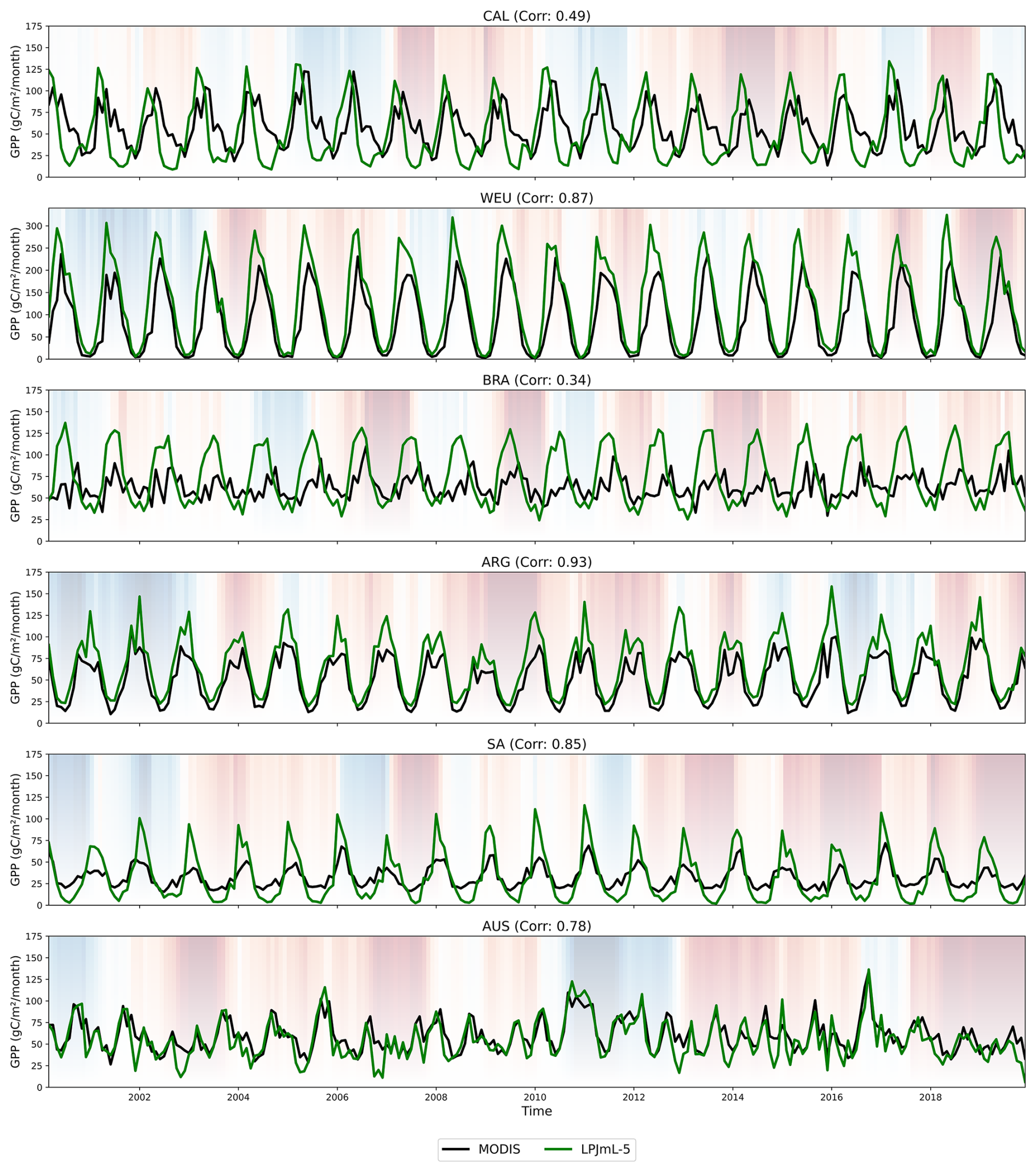
Figure 4 Time series of the GPP for LPJmL-5 with prescribed land cover (green) and MODIS (black) for the focus regions: California (CAL), western Europe (WEU), Brahmaputra (BRA), middle Argentina (ARG), southern Africa (SA) and the Murray Darling Basin in Australia (AUS). SPEI-12 is shaded in the background, where red areas indicate drier periods and blue areas wetter periods. Additionally, the figure includes the correlation between MODIS and LPJmL-5 per region. Note that WEU uses a different y axis range from the other regions.

3.1.2 Evaluating model performance with the GPP time series

Figure 4 shows the monthly GPP for LPJmL-5 (with prescribed land cover) and MODIS across the six focus regions between 2000 and 2019. The background shading represents the SPEI-12, highlighting dry periods in red and wet periods in blue. Additionally, the figure includes the correlation between MODIS and LPJmL-5.

Three general patterns can be identified in the time series: (1) A temporal shift in the LPJmL-5 GPP time series, with peaks occurring earlier in the season compared to MODIS; (2) Overestimation of summer GPP peaks, and in some cases underestimation of winter values; (3) Lower model performance during dry periods.

These patterns are reflected to varying degrees across the focus regions. CAL and BRA show the temporal shift, which may be the cause of the lower correlation with MODIS. BRA and WEU exhibit overestimation of summer GPP peaks, with SA also showing the underestimation of winter values. ARG performs relatively well, although it also shows slightly increased summer peaks. In AUS, the contrast between wet and dry periods is largest, with GPP simulated accurately during wet periods, while the model does not capture dry periods well. Despite these issues, WEU, ARG, SA, and AUS show relatively high correlation values, indicating that LPJmL-5 generally captures the seasonal and interannual patterns of satellite-derived GPP in these regions. Overall, based on the KGE values and the time series analysis, we can conclude that LPJmL-5 simulates GPP reasonably well, although notable regional differences remain.

3.2 General drought response

To evaluate the ability of LPJmL-5 to capture vegetation drought response, we applied the extreme-based method (Sect. 2.4). This method identifies the dominant drought timescale, defined as the SPEI timescale (ranging from 1 to 24 months) that has the most negative impact on vegetation during drought periods.

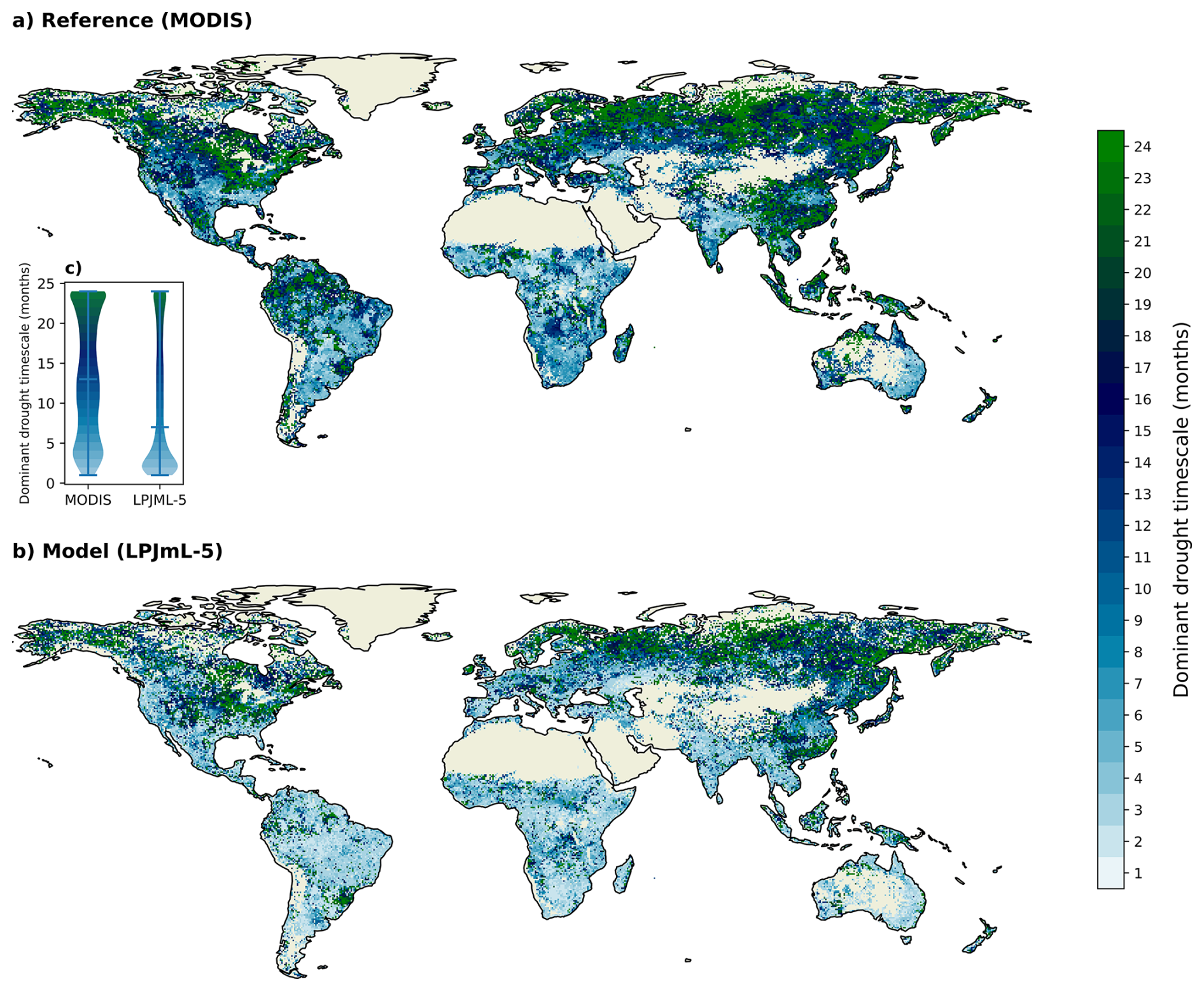
Figure 5 Spatial patterns of the dominant drought timescale of GPP_SA for (a) the MODIS reference and (b) the LPJML-5 model. The dominant timescale is defined as the shortest SPEI timescale (between 1 and 24 months) that shows the most negative GPP_SA during drought periods (with a SPEI threshold of −1). Bare areas and sparse vegetation are filtered out. (c) Violin plot comparing the distribution of dominant drought timescales between MODIS and LPJmL-5.

The spatial distribution of dominant drought timescales, shown in Fig. 5, shows a clear difference between MODIS (a) and the LPJmL-5 simulations (b). Compared to MODIS, LPJmL-5 exhibits shorter dominant timescales, indicating a faster GPP response to drought. This difference is most pronounced in the Southern Hemisphere. LPJmL-5 also shows a skewed distribution with a clear peak around 2 months (panel c), whereas the MODIS response is more evenly distributed. Overall, these patterns highlight differences in temporal sensitivity between LPJmL-5 and the satellite-derived reference, with LPJmL-5 showing shorter response times during drought periods.

3.3 MYD and ND response

After evaluating LPJmL-5's response to droughts in general, this study now shifts its focus to MYDs and NDs.

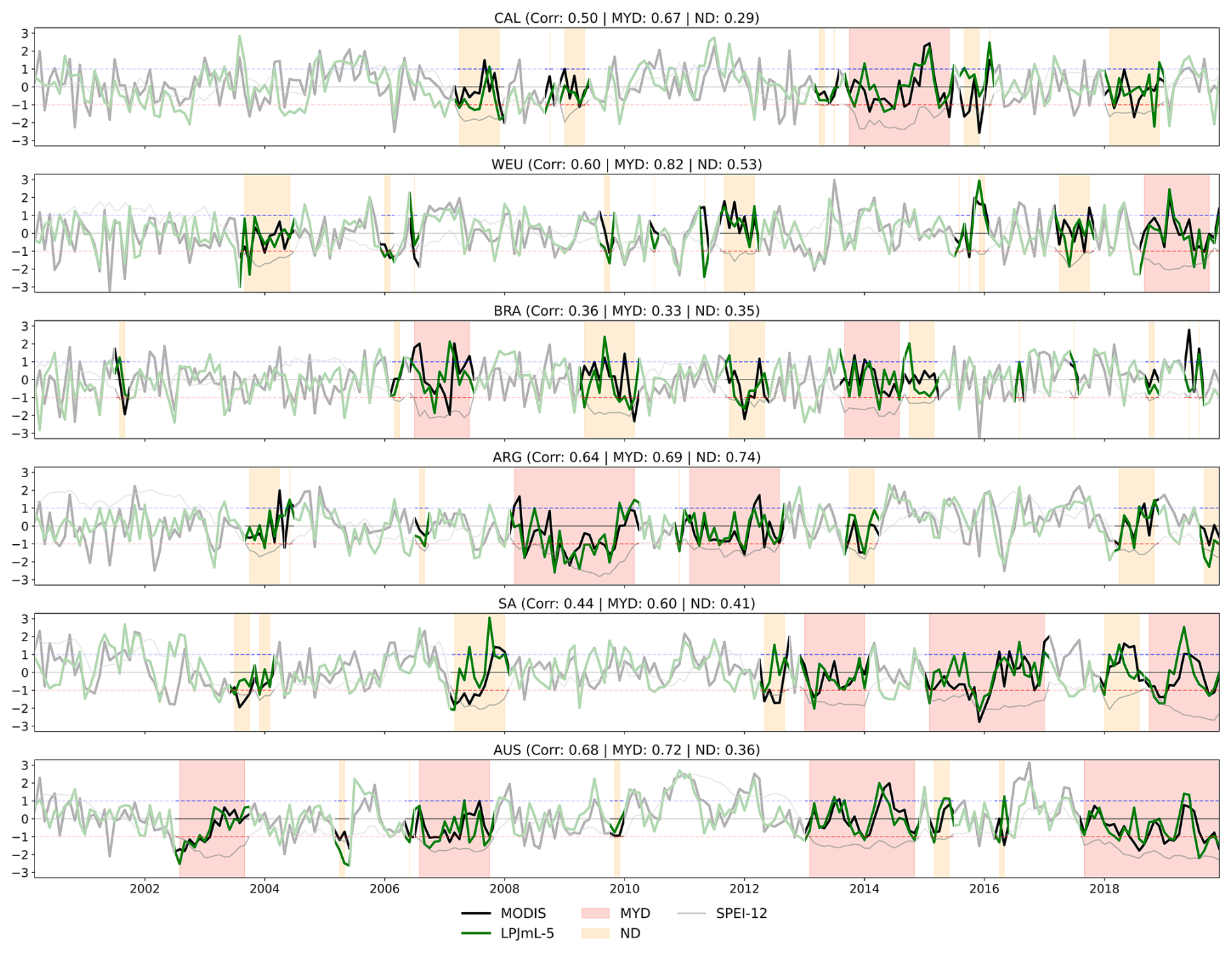
Figure 6 Timeseries of GPP_SA for LPJmL-5 and MODIS. MYDs and NDs are shaded in red and orange, respectively. Correlation coefficients between LPJmL-5 and MODIS are shown for the full time series, MYDs, and NDs. The grey line indicates the SPEI-12. The red and blue dashed lines mark −1 and +1, respectively.

3.3.1 Temporal patterns

Firstly, we examine how well LPJmL-5 captures the timing and magnitude of GPP_SA during MYDs and NDs across the focus regions. Figure 6 shows the time series of GPP_SA for the satellite-derived reference (MODIS) and LPJmL-5, with MYDs and NDs indicated by red and orange shaded areas, respectively.

Overall, LPJmL-5 captures the timing and magnitude of GPP_SA anomalies reasonably well, showing relatively high correlations with MODIS in most regions. The model aligns particularly well in CAL, WEU, ARG, and AUS, while performance is somewhat lower in SA and BRA. Correlations during MYDs are higher than those for the entire time series in all regions except BRA, and generally higher than those during NDs, except in ARG and BRA. This suggests that LPJmL-5 simulates MYD dynamics more accurately than ND dynamics.

Nonetheless, some systematic differences remain during MYDs: (1) the model tends to simulate a too fast and severe decline in GPP_SA at the onset of MYDs, and (2) it exhibits strong variability during MYD periods, especially in the form of abrupt recovery spikes that are not seen in the satellite-derived reference.

These biases are reflected across the focus regions to varying degrees. In WEU, the model simulates an early GPP_SA drop that precedes the reference onset. CAL shows a similar offset, likely linked to the timing mismatch seen in Fig. 4. In BRA, the first MYD minimum occurs too early in the model, while the second MYD ends with a sudden increase in GPP_SA not seen in the reference, again indicating an early response and rapid recovery. ARG captures drought severity relatively well but still shows some abrupt recovery spikes during MYDs. SA also shows the rapid onset and overestimated recovery rate, despite persistently low SPEI-12 values. AUS shows the best overall agreement, with most MYDs being captured well. However, the second MYD still shows the strong variability mid-drought, though less severely.

Overall, while LPJmL-5 tends to simulate an overall more dynamic response with faster declines and rapid recovery during MYDs, it successfully reproduces the key temporal dynamics of MYDs relative to the satellite-derived reference.

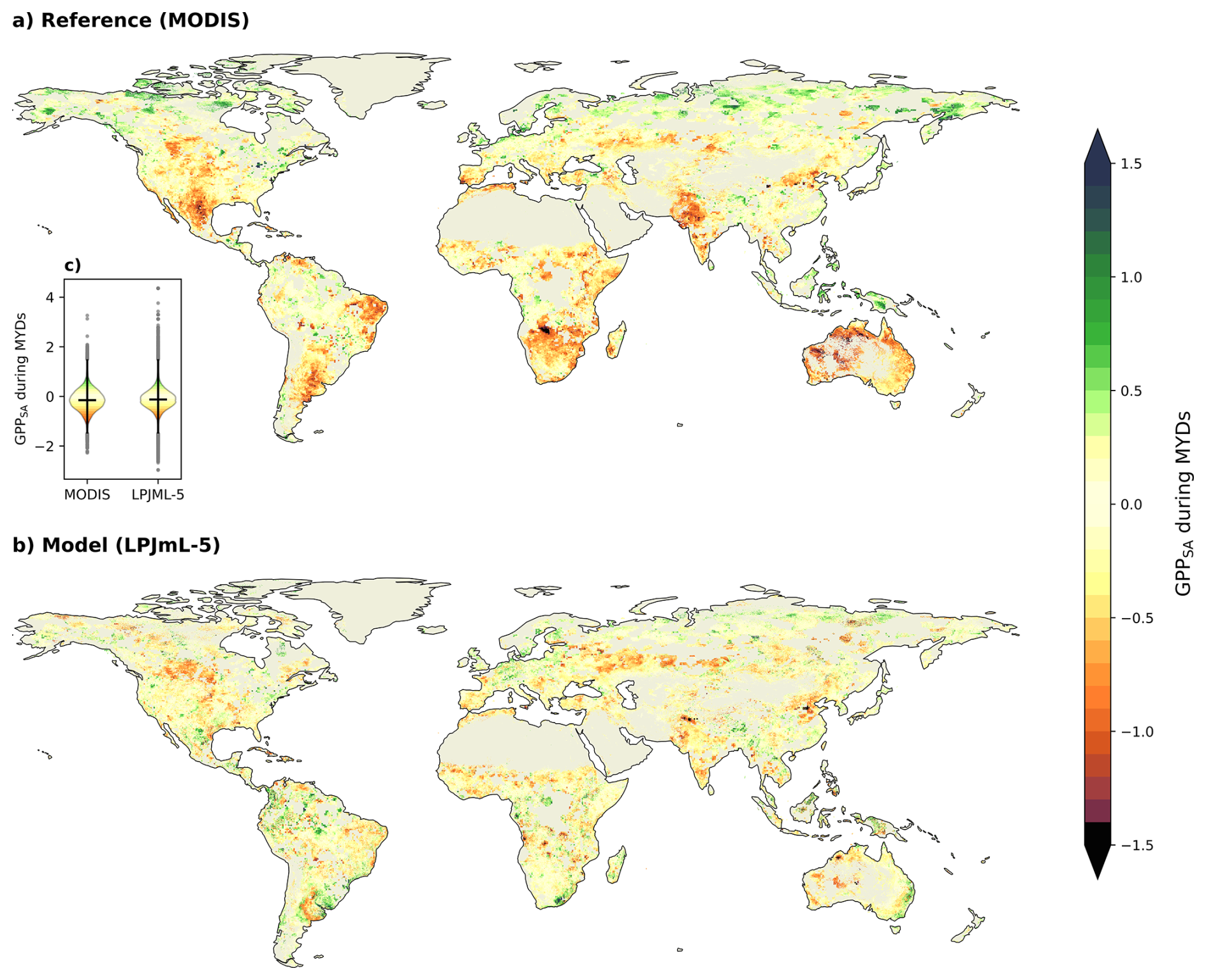
Figure 7 Spatial pattern of the mean GPP_SA during MYDs for (a) MODIS and (b) LPJmL-5. Positive values indicate higher GPP than normal during MYDs, while negative values indicate reduced GPP values. Bare areas and sparse vegetation are filtered out. (c) shows a violin plot comparing the distributions of the mean GPP_SA during MYDs from MODIS and LPJmL-5.

3.3.2 Spatial patterns

In addition to the regional time series analysis, we now examine global spatial patterns of vegetation response to MYDs. Figure 7 shows the spatial distribution of the mean GPP_SA during MYDs, as derived from (a) the MODIS reference and (b) the LPJmL-5 model. Negative values (red) indicate below-average GPP during MYD periods, while positive values (green) indicate GPP being higher than average.

Overall, LPJmL-5 simulates less severe GPP_SA during MYDs compared to MODIS. However, the Spearman rank correlation (0.326, p<0.001) still indicates a similarity in the overall spatial patterns between the model and the reference. This means that the model captures some important hotspot areas, but there are still noticeable differences. We attribute these differences largely to the abrupt recovery events in the model, as seen in Fig. 6. The violin plot (Fig. 7c) shows that MODIS has a slightly lower median. However, LPJmL-5 displays more extreme values at both ends of the distribution, indicating greater variability in the modelled MYD responses.

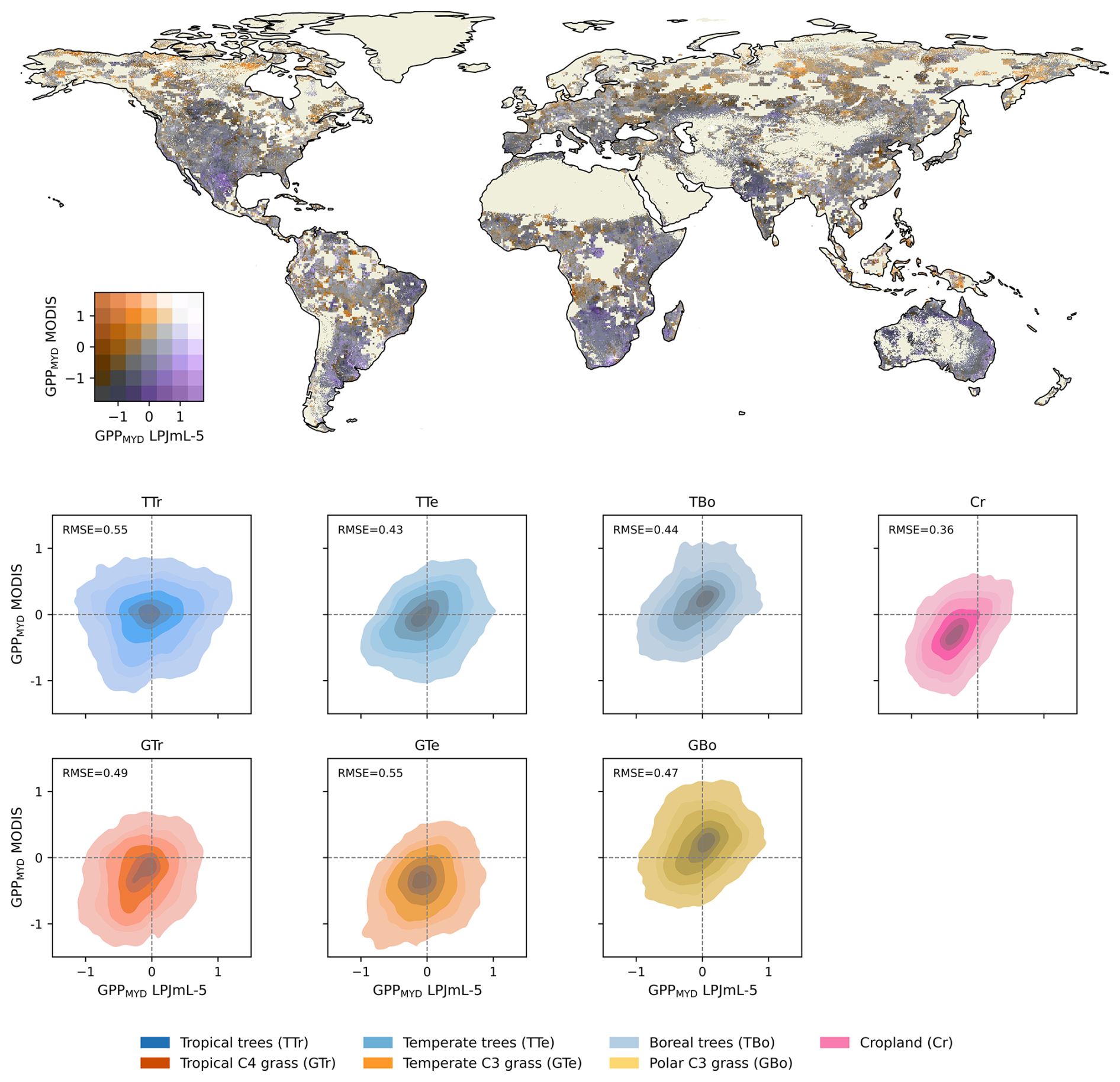
Figure 8 Spatial differences in mean GPP_SA during MYDs between MODIS and LPJmL-5. The map highlights regions where LPJmL-5 shows weaker or stronger vegetation responses relative to the satellite-derived reference. Purple shades indicate underestimated negative impacts, while orange shades indicate underestimated positive or overestimated negative impacts. White, grey and black shades represent regions where the model and reference agree closely on vegetation response during MYDs. Insets display two-dimensional kernel density estimates (KDEs) for seven vegetation types, illustrating the distribution of differences in mean MYD responses. KDE levels are set to [0.05, 0.15, 0.25, 0.5, 0.75, 0.9, 1.0]. Root mean square error (RMSE) for each plant functional type is included in the insets.

To further highlight these differences, Fig. 8 shows the spatial difference in mean GPP_SA during MYDs between MODIS and LPJmL-5 and two-dimensional Kernel Density Estimate (KDE) plots for the different PFTs. Purple shades indicate underestimation of negative drought impacts, while orange shades indicate underestimation of positive impacts or overestimation of negative impacts. Black, grey and white areas indicate close agreement between the model and the reference.

LPJmL-5 shows a reasonable agreement with MODIS in most regions, as indicated by the black, grey and white areas. These areas include Central North America, Europe, and parts of East and West Asia. However, there are several regions that emerge as hotspots of LPJmL-5 underestimation of GPP anomalies (visible as dark purple areas), including Australia, Northwest India, Pakistan, Southern Africa, Central Argentina, Eastern Brazil, and Northern Mexico. In these regions, LPJmL-5 shows weaker or absent negative responses, suggesting that the model does not fully capture drought severity in these areas. This finding is consistent with the temporal patterns shown in Fig. 4. Additionally, LPJmL-5 tends to underestimate the satellite-derived positive GPP responses in the arctic boreal zone (visible as orange areas). Here, the model does not reproduce the positive GPP anomalies during MYDs seen in the MODIS reference data (Fig. 7 and Ruijsch et al., 2025).

Beyond spatial patterns, differences between LPJmL-5 and MODIS also vary by PFT (Fig. 8). Tropical trees show a wide spread in MYD GPP responses, while temperate trees align more closely with MODIS but still occasionally underestimate negative impacts (lower right quadrant). Grasslands show reasonable agreement, with LPJmL-5 capturing most directions of the MYD response correctly. Croplands, although displaying the weakest agreement in absolute GPP (Fig. 3), show strong agreement in drought-induced GPP anomalies. This is reflected by the lowest RMSE among all PFTs (Fig. 8). This indicates that, despite limitations in simulating absolute productivity, LPJmL-5 more consistently captures the relative response of croplands to drought events.

Overall, LPJmL-5 reproduces several key temporal and spatial MYD patterns present in the MODIS reference, but still shows some model bias in both time and space. Temporally, LPJmL-5 often simulates faster and stronger vegetation declines at the onset of the MYD than the satellite-derived reference and shows a fast recovery during the drought period. Spatially, LPJmL-5 shows a reasonable agreement with MODIS in most regions and for most PFTs, but also shows some underestimation of both strong negative and strong positive vegetation responses. These biases may be caused by short-term overreactions and rapid recoveries in the model's time series, which reduces the average drought response.

4 Discussion

Overall, this study assesses LPJmL-5's ability to simulate global vegetation responses to (multi-year) droughts. First, comparing dynamic and prescribed land cover settings in LPJmL-5 revealed that prescribed land cover improves agreement with MODIS GPP. The lowest agreement is generally found in the Southern Hemisphere and in cropland-dominated regions. Second, LPJmL-5 and MODIS GPP exhibit similar broad seasonal and interannual variability, although the model tends to simulate stronger GPP dynamics and introduces temporal shifts relative to the satellite-derived reference. Third, using the extreme-based method to identify the timescale at which drought has the strongest impact on vegetation, we found that LPJmL-5 simulates shorter dominant drought timescales than MODIS, particularly in tropical regions and the Southern Hemisphere, indicating a faster modelled GPP response to drought conditions. Fourth, the analysis of MYDs revealed a consistent pattern of model bias across both time and space. Temporally, LPJmL-5 simulates stronger and more rapid GPP declines at the onset of MYDs and shows faster recovery during drought periods compared to the reference. Spatially, the model shows muted representations of both strong negative and strong positive GPP anomalies compared to MODIS.

Overall, LPJmL-5 simulates faster GPP declines and recoveries during droughts than the satellite-derived reference, suggesting limitations in how the model represents vegetation resistance and resilience to water-induced stress and mortality.

4.1 Uncertainties in the model choices and setup

Different choices in model parametrisation and setup can lead to significant differences in modelled GPP. For example, both the choice of meteorological forcing dataset (ERA5 (Hersbach et al., 2023) vs. W5E5 (Lange et al., 2022)) and the temporal resolution (monthly vs. daily) have a significant impact on simulated GPP patterns (Sect. S4). This indicates that it is important for future drought oriented studies to make clear choices with regard to the modelling setup. In this study, we selected the daily W5E5 dataset (Lange et al., 2022), as it is bias-corrected and offers a high temporal resolution and the total global GPP was closest to that found in observational datasets.

Our analyses also showed that GPP output is highly sensitive to the radiation inputs (Sect. S4). GPP values varied substantially depending on whether the model calculated radiation internally or used observed radiation data. We found that errors in GPP are higher from internal estimation, compared to directly providing longwave and shortwave radiation from observations.

Using dynamic land cover in LPJmL-5 resulted in systematically overestimated GPP values across most regions (Fig. 2 and Sect. S5), also noted in Schaphoff et al. (2018a). We argue that this difference is the result of a mismatch between modelled and observed vegetation distributions (Appendix C and Sect. S5), which is to be expected as the land cover is not constrained to the observed land cover. For example, LPJmL-5 simulates tree cover in parts of Western Europe where forests could exist naturally, but are absent today due to long-term human management. To better match satellite-derived GPP and reduce these discrepancies, we prescribed land cover fractions, rather than letting the model simulate land cover dynamically.

4.2 Evaluation of GPP simulations and vegetation drought response in LPJmL-5

Prescribing land cover in LPJmL-5 improved the agreement with MODIS GPP, as indicated by higher KGE values in Fig. 2. This is consistent with studies showing that accurate land cover representation is essential for reproducing observed productivity patterns (Krause et al., 2022), and that constraining DGVM simulations with satellite-derived observations (including land cover) enhances their ability to capture observed spatial patterns of vegetation and carbon dynamics (Forkel et al., 2019).

Breaking down the differences between LPJmL-5 and MODIS GPP during MYDs by vegetation type further highlights a varying model performance (Fig. 8). Tropical trees show the largest variability in drought response, showing both under- and overestimations of impacts. Similar results were found by Powell et al. (2013), who showed that terrestrial biosphere models underestimate drought impacts on tropical forest biomass. Temperate trees generally align more closely with observations but still underestimate negative drought impacts. This is consistent with Kolus et al. (2019), who found that land carbon models underestimate the severity and duration of drought effects on productivity across temperate forests in the US and Europe. Similarly, Schaefer et al. (2012) observed that models frequently overpredict GPP under dry conditions, further pointing to an underestimation of drought stress. Boreal trees and grasses are more prone to underestimated positive responses. Croplands, despite poorer agreement in absolute GPP dynamics, show comparatively better agreement in drought-induced anomalies. This suggests that while LPJmL-5 struggles to reproduce the magnitude of the GPP, it is able to capture relative deviations during drought events. Such behaviour indicates that biases in absolute GPP do not necessarily translate into errors in anomaly-based responses.

A key limitation underlying these issues appears to be how vegetation mortality is represented in LPJmL-5. In the model, mortality is only driven by low productivity and heat stress, and can not be directly induced by prolonged water deficits. Drought-induced mortality occurs only if plants fail to produce enough biomass to sustain themselves. However, this natural mortality is capped by a maximum annual rate (Schaphoff et al., 2018b), which restricts how much vegetation can be lost due to die-off each year. Moreover, this mortality mechanism is only active in the dynamic land cover setting, and is not applied when land cover is prescribed. Since the simulations in this study use the prescribed land cover setting, no vegetation is lost due to this background mortality. This means that while GPP may decline sharply during droughts, vegetation does not die, causing unrealistically rapid recovery periods when precipitation (temporarily) returns. Although LPJmL-5 includes a heat-stress mortality mechanism, it only applies to boreal trees (Schaphoff et al., 2018b). As a result, vegetation decline during MYDs is not directly driven by water shortages, which prevents large-scale die-off and causes the model to underestimate total vegetation loss. These limitations reduce the model's ability to simulate the full severity of vegetation decline, especially during MYDs. This issue has been noted by Schaphoff et al. (2018a), who reported that the lack of realistic mortality processes leads to an overestimation of simulated biomass and contributes to biases in GPP. Similarly, McDowell et al. (2013) found that models which combine carbon starvation with hydraulic failure mechanisms are better able to reproduce observed drought-induced tree mortality, and Zhou et al. (2013) highlighted the need to account for both stomatal and non-stomatal limitations to realistically capture plant responses to water stress. Meyer et al. (2025) further showed that including hydraulic processes in LPJ-GUESS improves simulations of drought responses. Together, these findings suggest that LPJmL-5 likely underestimates the true impact of drought on vegetation.

Despite underestimating long-term vegetation loss, LPJmL-5 tends to overestimate vegetation decline at the start of droughts, as shown in Figs. 5 and 6. LPJmL-5 does include a water stress factor that influences the growth, which results in a rapid decline in GPP. This stress is determined by soil moisture availability and fixed rooting depths for each PFT, without accounting for dynamic rooting strategies, capillary rise or explicit groundwater processes (Schaphoff et al., 2018b). However, in reality, vegetation often withstands short-term stress periods through drought survival strategies (Santiago et al., 2016; Pivovaroff et al., 2016). At the same time, LPJmL-5 also simulates unrealistic recoveries during the drought period. Since there is no mortality, vegetation can survive during a drought period, resulting in no loss of biomass. When conditions improve temporarily, for example due to brief rainfall, the model quickly simulates regrowth. This leads to an unrealistic drought recovery effect. This is in contrast with real vegetation, which often suffers from long-term impacts (Wu et al., 2018). Both the quick decline and recovery are consistent with findings by Kolus et al. (2019), who show that land carbon models underestimate the severity and duration of drought impact on plant productivity.

Together, the combination of overly sensitive short-term GPP decline, limited representation of long-term vegetation loss, and unrealistically fast recovery during drought periods results in a mismatch in LPJmL-5's simulated vegetation drought response. While prescribing land cover improves the overall GPP performance, these structural issues in the mortality representation limit the model's ability to simulate realistic vegetation dynamics during drought events. This is especially limiting when the analysis is focused on multi-year drought events, which have been shown to cause higher vegetation mortality rates (Češljar et al., 2025) and are expected to become more frequent under climate change (Wiel et al., 2022).

4.3 Uncertainties in methodological choices

To improve the overall quality and reliability of our simulations, we used the state-of-the-art dynamic vegetation model LPJmL-5. This model is publicly available with an extensive model description and evaluation (Schaphoff et al., 2018b, a; von Bloh et al., 2018). LPJmL-5 provides a multitude of vegetation-related outputs on ecological, hydrological, and agricultural components, making it suitable for studying vegetation responses at the global scale.

Drought events were identified using the Standardized Precipitation Evapotranspiration Index (SPEI), which incorporates both precipitation (P) and potential evapotranspiration (PET), allowing it to better reflect the impact of temperature on drought severity (Vicente-Serrano et al., 2010). As a standardized index, SPEI also enables consistent spatial comparisons of drought conditions at the global scale. By using a 12 month aggregation period for the SPEI, we also remove seasonal variations and focus on capturing MYDs.

As a standardized metric, SPEI characterizes drought conditions relative to the local climatic baseline, reflecting periods that are characterized by below normal water availability. In energy-limited regions, such as the tropics or boreal forests, negative SPEI values may occur even when absolute water availability remains relatively high (Zang et al., 2019). To ensure these droughts correspond to meaningful reductions in water availability, we compared soil water content (SWC) during droughts and normal conditions (Sect. S2), finding consistently lower SWC across soil layers. This supports the interpretation that identified MYDs correspond to periods of meaningful vegetation stress, even in energy-limited regions.

While there is currently no universally agreed-upon definition of MYDs, we follow the approach of Wiel et al. (2022) (see Sect. 2.1), which was also adopted in Ruijsch et al. (2025) and van Mourik et al. (2025). SPEI values are sensitive to the method and input data used for calculating PET. We compared results using ERA5 and W5E5 and found differences in the number of MYDs identified for the period 2000–2019 (Sect. S4). Nonetheless, the MYDs identified in our focus regions are broadly consistent with those reported in other studies (van Mourik et al., 2025; Wiel et al., 2022; Luo et al., 2017; Liu et al., 2022; Chikoore and Jury, 2021; Naumann et al., 2023; van Dijk et al., 2013), despite minor differences in timing.

To evaluate vegetation responses, we used monthly MODIS GPP as a proxy for ecosystem productivity, representing the amount of carbon captured from the atmosphere through photosynthesis (Beer et al., 2010). Previous drought studies have often relied on the EVI (Ruijsch et al., 2025; Huang and Xia, 2019; Yang et al., 2024), but EVI is satellite-derived and not directly available from LPJmL-5. Because MODIS GPP and EVI are strongly correlated (Rahman et al., 2005; Sims et al., 2006; see also Sect. S3), including during multi-year droughts (Ruijsch et al., 2025), MODIS GPP can be considered a suitable proxy for vegetation activity.

Several studies further indicate that MODIS GPP provides a meaningful representation of productivity across biomes, with most errors linked to input datasets rather than the algorithm itself. Performance is generally good in temperate and mixed forests, while errors are larger in evergreen broadleaf forests and tropical regions (Tang et al., 2015). Wang et al. (2017) showed that much of the error originates from FPAR, land-cover misclassification, and light-use efficiency parameters rather than meteorology. Systematic underestimation has also been reported in grasslands (Zhu et al., 2018). These studies agree that cloud contamination and uncertainties in tropical regions remain key challenges. Taken together, the strong correspondence between MODIS GPP, EVI, and solar-induced fluorescence (Sect. S3) supports the use of MODIS GPP as our validation dataset for LPJmL-5 GPP, while acknowledging that performance is weaker in tropical ecosystems and that results should be interpreted with these limitations in mind.

Although other sources of GPP data exist, such as site-level flux tower measurements, we choose to use satellite-derived MODIS GPP because it provides consistent, observation-based estimates at the global scale. To maintain observational consistency and avoid mixing in other models, we did not include GPP estimates derived from other land surface models as they are likely based on similar assumptions and equations as the LPJmL-5 model. Nonetheless, MODIS GPP is subject to uncertainty, particularly in tropical regions (Sect. S3), and this should be kept in mind when interpreting the results.

5 Conclusion

This study evaluated LPJmL-5's ability to simulate global vegetation responses to drought using MODIS-derived GPP as a reference. Our analysis shows that LPJmL-5 simulates shorter response times to drought than observed by MODIS, particularly in tropical regions and the Southern Hemisphere. During MYDs, LPJmL-5 captures the key temporal and spatial dynamics found in MODIS. However, the model tends to overestimate vegetation response at the MYD onset and shows rapid recovery behaviour. This results in muted overall drought impacts and an underrepresentation of both strong negative and strong positive GPP anomalies.

Among PFTs, croplands show the best agreement with satellite-derived MYD responses. In contrast, boreal vegetation shows underestimated positive drought responses and temperate vegetation underestimated negative ones. Tropical vegetation displays more mixed results, with both over- and underestimation. These differences between modelled and satellite-derived GPP during drought periods may be partly attributed to how LPJmL-5 represents vegetation stress and drought-induced mortality. In particular, while the model responds strongly to short-term reductions in productivity, it limits long-term vegetation decline, leading to rapid recovery and reduced vegetation die-off during drought periods.

Beyond drought conditions, prescribing land cover instead of simulating it dynamically improves the model's ability to reproduce global GPP dynamics. Overall, LPJmL-5 reproduces GPP reasonably well, although performance declines in parts of the Southern Hemisphere and in cropland-dominated regions. This suggests that general GPP simulation performance is not necessarily linked to performance during drought conditions.

In conclusion, LPJmL-5 is able to reproduce several key features of vegetation responses to MYDs, but tends to simulate vegetation that is too responsive during both the drought onset and the recovery. This points to limitations in the representation of vegetation resistance and resilience to water stress and mortality. Improving these processes is important to more accurately capture the magnitude of drought impacts and for strengthening confidence in model-based assessments of vegetation responses to droughts.

Appendix A: Dominant land cover types

Figure A1 shows the dominant land cover types at a 0.1° spatial resolution, based on LPJmL-5's land cover and land use dataset (see Table 1). Cropland fractions were combined into a single “cropland” category, while natural PFTs were grouped into broader vegetation classes: tropical trees (tropical broadleaved evergreen and raingreen trees), temperate trees (needleleaved evergreen, broadleaved evergreen, and broadleaved summergreen trees), boreal trees (needleleaved evergreen, broadleaved summergreen, and needleleaved summergreen trees), tropical C₄ grass, temperate C₃ grass, and polar C₃ grass.

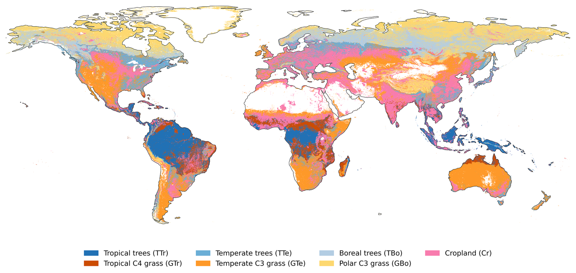
Figure A1 Dominant land cover types at a 0.1° resolution for 2019. Vegetation categories include tropical trees (TTr), temperate trees (TTe), boreal trees (TBo), cropland (Cr), tropical C₄ grass (GTr), temperate C₃ grass (GTe), and polar C₃ grass (GBo).

Appendix B: Number of MYDs and chosen focus regions

Figure B1 shows the number of MYDs (2000–2019) at a 0.5° spatial resolution from W5E5 data (Lange et al., 2022) (see Sects. 2.1 and S1). Black outlines indicate the chosen focus regions: California (CAL), the Rhine-Meuse delta in western Europe (WEU), the Brahmaputra River basin in Bangladesh/India/Bhutan/China (BRA), central Argentina (ARG), the Orange River basin in southern Africa (SA), and the Murray-Darling basin in Australia (AUS) (see Sect. 2.6).

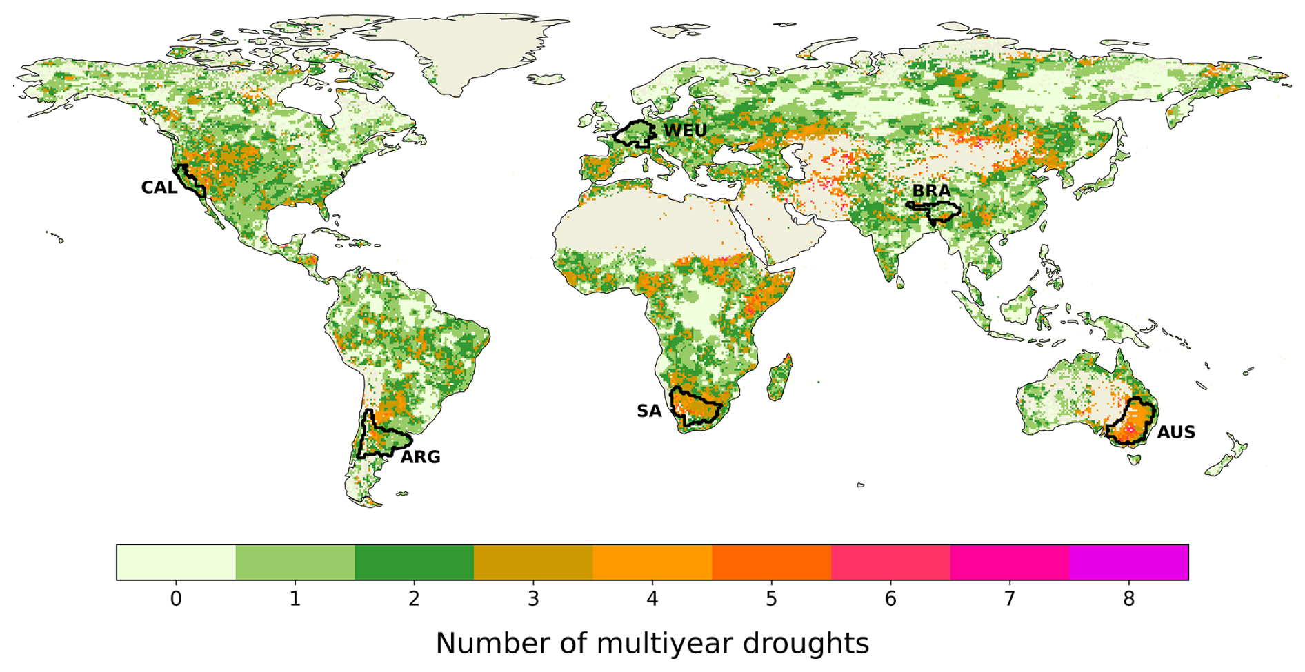
Figure B1 Number of MYDs between 2000–2019 at 0.5° spatial resolution. Bare areas and regions with sparse vegetation are excluded. Black contours indicate the six chosen focus regions: CAL, WEU, BRA, ARG, SA, and AUS.

Appendix C: LPJmL dynamic vs. ESA prescribed land cover

Figure C1 shows the difference in vegetation cover fractions between LPJmL-5 and ESA. Globally, the ESA dataset shows greater coverage of temperate and polar C₃ grasses, as well as boreal needleleaved summergreen forests. In contrast, LPJmL-5's dynamic vegetation simulates more temperate needleleaved evergreen trees, boreal needleleaved evergreen trees, boreal broadleaved summergreen trees, and tropical C₄ grasses.

The CDFs in Fig. C2 further show the impact of land cover on model performance. Across all vegetation types, the prescribed land cover shows higher KGE values. The difference between prescibed and dynamic land cover is particularly pronounced for temperate C₃ grasses, which perform poorly with the the dynamic land cover. LPJmL-5 substantially underrepresents the spatial extent of temperate C₃ grasses, assigning them to only 2.7 % of grid cells, compared to 22.2 % under the ESA-based classification. This mismatch likely contributes to the poor performance, as misclassified vegetation types lead to unrealistic GPP estimates. Tree-dominated grid cells also show better performance with prescribed land cover, however, the difference is less severe than for grasses.

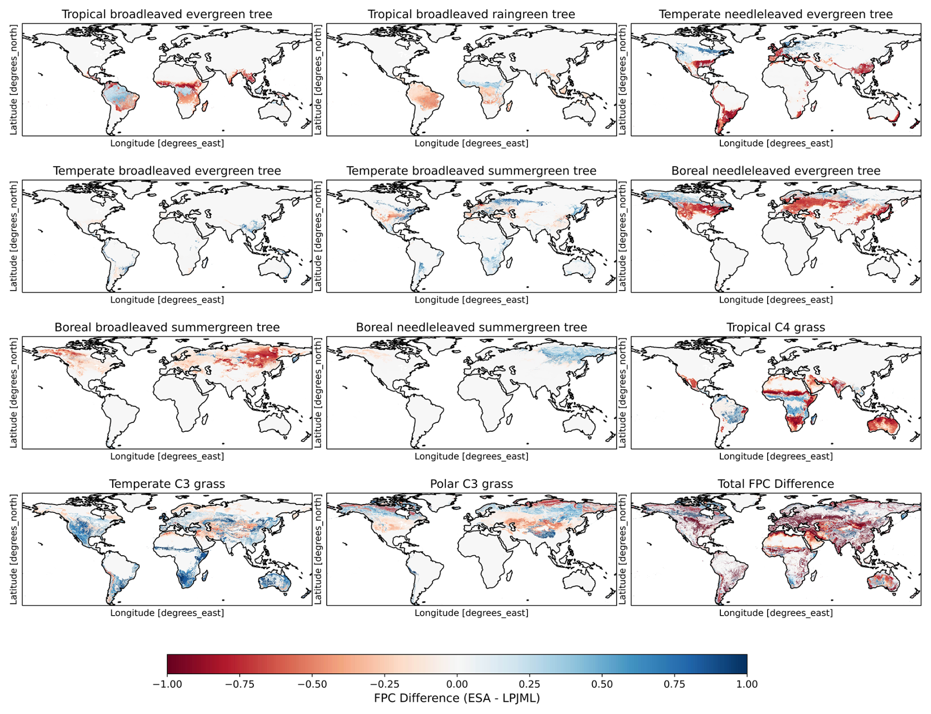
Figure C1 Difference in vegetation cover fractions between LPJmL-5 and ESA. Blue areas indicate where ESA has a higher vegetation fraction; red areas indicate where LPJmL-5 simulates a higher vegetation fraction.

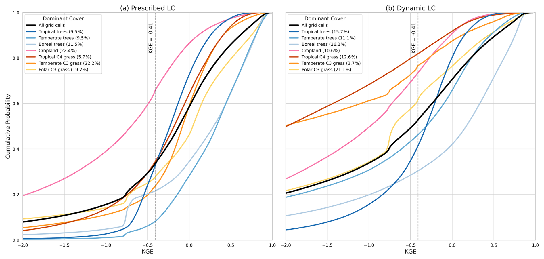
Figure C2 Cumulative distribution function (CDF) of the KGE of the (a) prescribed land cover GPP and (b) dynamic land cover for the different vegetation types in LPJmL-5. Percentages show the percentage of grid cells with that land cover. Black dashed line indicates KGE $=-\mathrm{0.41}$. Values greater than −0.41 indicate that the model improved upon the mean benchmark.