Developing Guidelines for working with Multi-Model Ensembles in CMIP

Earth System Models (ESMs) are a key tool for studying the climate under changing conditions. Over recent decades, it has been established to not only rely on projections of a single model but to combine various ESMs in multi-model ensembles (MMEs) to improve robustness and quantify the uncertainty of the projections. The data access for MME studies has been fundamentally facilitated by the World Climate Research Programme's Coupled Model Intercomparison Project (CMIP) – a collaborative effort bringing together ESMs from modelling communities all over the world. Despite the CMIP standardization processes, addressing specific research questions using MMEs requires unique ensemble design, analysis, and interpretation choices. Based on the collective expertise within the Fresh Eyes on CMIP initiative, mainly composed of early-career researchers engaged in CMIP, we have identified common issues and questions encountered while working with climate MMEs. Here, we provide a comprehensive literature review addressing these questions. We provide statistics tracing the development of the climate MMEs analysis field throughout the last decades, and, synthesizing existing studies, we outline guidelines regarding model evaluation, model dependence, weighting methods, and uncertainty treatment. We summarize a collection of useful resources for MME studies, we review common questions and strategies, and finally, we outline emerging scientific trends, such as the integration of machine learning (ML) techniques, single model initial-condition large ensembles (SMILEs), and computational resource considerations. We thereby aim to support researchers working with climate MMEs, particularly in the upcoming 7th phase of CMIP.

1 Introduction

Earth system models (ESMs) are a key tool for assessing the future climate under changing conditions. Starting from the seminal work of Manabe and Hasselmann (e.g. Manabe and Strickler, 1964; Manabe and Bryan, 1969; Manabe and Wetherald, 1967; Hasselmann, 1976), who were awarded the 2021 Nobel Prize in Physics, climate models have continuously evolved over decades. During this process, models have become progressively more complex, encapsulating processes related to aerosols, atmospheric chemistry, the carbon cycle, and ocean biogeochemistry. This evolution occurred in parallel with advances in Earth system observations, high-resolution numerical models giving insight into smaller-scale phenomena (e.g., detailed radiative transfer models, cloud-resolving models, large-eddy simulations), and growing computational power (e.g. Gettelman et al., 2022; Schneider et al., 2017) allowing model resolution to steadily improve.

Since the beginning of large-scale atmospheric modelling, intercomparisons among models have been carried out. Initially, this intercomparison was mostly performed for numerical weather prediction as computational resources limited the intercomparison of studies in the climate context, and a clear experimental strategy was lacking (Gates, 1992). Since the 1970s, the Working Group on Numerical Experimentation (WGNE), supporting the World Climate Research Programme, has organized several intercomparison projects among climate models. The first international systematic intercomparison framework for climate models was established in 1990 in the context of the Atmospheric Model Intercomparison Project (AMIP; Gates, 1992). In the early 1990s, the Intergovernmental Panel on Climate Change (IPCC) provided an intercomparison of atmospheric models in their first assessment report (AR; Gates, 1992). In the following years, Räisänen (1997) advocated the need for quantitative model comparison and raised the thought that the agreement between models can indirectly serve as a measure for the reliability of the simulations. Accordingly, Räisänen and Palmer (2001) introduced a probabilistic perspective on MME projections. The authors quantified the probability of specific climate events happening based on 17 coupled atmosphere-ocean general circulation models (AOGCMs). Contemporaneously, AMIP was followed by the Coupled Model Intercomparison Project (CMIP) coordinated by the World Climate Research Programme (WCRP), which also incorporated results from AOGCMs (Meehl et al., 2000).

While the first phase of CMIP was limited to control runs, new standardized scenarios were incorporated throughout the phases of CMIP with an increasing number of international model centres contributing simulations. Concurrently, the volume of data has been steadily increasing (Williams et al., 2016) and is stored within a standardized format at the Earth System Grid Federation (ESGF) central repository (Cinquini et al., 2012). In more recent CMIP generations, a variety of supporting experiments is conducted (e.g. Eyring et al., 2016), including paleoclimate runs (simulations of the `distant past'), historical runs (simulations of the “recent past”), control runs to study natural variability, as well as various experiments. Finally, future climate change simulations are performed for various greenhouse gas emission scenarios such as abrupt carbon dioxide doubling or quadrupling to derive climate sensitivity (measure of how much the Earth's climate system will warm under a doubling of atmospheric CO₂ concentration), as well as for multiple plausible future emission scenarios (O'Neill et al., 2017; Riahi et al., 2017; van Vuuren et al., 2025). The latter denote diverse scenarios of evolution of the global society (including population, economy, and technology) which thus lead to differing emissions of greenhouse gases (CO₂, CH₄, NO₂) and other air pollutants until the end of the 21st century and are associated with different climate change mitigation and adaptation policies and challenges (IPCC, AR6). These CMIP projections have proven essential for informing mitigation and adaptation strategies to climate change at the global and regional scales (Meehl et al., 2000). For regional analysis, the CMIP output is often downscaled to finer resolution, e.g. by using the CMIP output as boundary conditions for regional climate models (RCMs). This is done e.g. in the WCRP COordinated Regional climate Downscaling EXperiment (CORDEX), which provides a coordinated framework for producing and evaluating regional climate projections across multiple domains worldwide (Giorgi, 2019; Gutowski et al., 2016)

The main components of an ESM describe the atmosphere, ocean, cryosphere, land, and increasingly, the carbon cycle and other biogeochemical processes. Each component involves a variety of interacting phenomena occurring at a wide range of spatial and temporal scales (e.g. Gettelman et al., 2022). In all ESMs, the continuous behavior of the atmosphere and ocean is first discretized in space and time via the so-called “model dynamical core” which encompasses known governing equations that capture resolved (grid-scale) phenomena and parameterization schemes that represent unresolved or poorly understood (subgrid-scale) processes. ESMs differ in the choice of computational grids (e.g., latitude-longitude structured grids, icosahedral grids, variable resolution cube-sphere grids), numerical methods for solving the dynamical core equations, and in parameterization schemes. While some parameterizations are based on well-established physical theory, others, particularly those related to clouds or turbulence, remain subject to substantial uncertainty. In addition, computational limitations restrict the accuracy with which models can represent certain relevant processes. Therefore, the decisions made at modelling centers make each ESM an imperfect attempt to represent a multitude of highly complex, nonlinear processes, and the synchronized interplay among them. Depending on the interest of the end user, some of these necessary idealization decisions may be more suitable than others.

Combining several ESMs to multi-model ensembles (MMEs) can have numerous advantages compared to individual simulations, e.g. to account for the uncertainty arising from the differing modelling decisions (model uncertainty). Starting in the weather forecasting community, numerous studies have shown the benefits of ensemble predictions compared to predictions based on single models (Doblas-Reyes et al., 2003; Krishnamurti et al., 1999), e.g. the North American MME showed improvements in various skill metrics (correlation, RMSE, RPSS, and reliability) compared to individual models used before (Kirtman et al., 2014). Inspired by these findings, studies in the climate context also analyzed the potential benefits from working with MMEs for projections. In climate model evaluation, the MME projections have proven to outperform individual model projections in numerous studies e.g. regarding the mean (Gleckler et al., 2008; Knutti et al., 2010a; Lambert and Boer, 2001; Palmer et al., 2005; Phillips and Gleckler, 2006; Pincus et al., 2008; Reichler and Kim, 2008) and variability (Zhang et al., 2007). The enhancement of the signal and cancellation of errors contribute to these advantages (Doblas-Reyes et al., 2005; Hagedorn et al., 2005; Smith et al., 2013). Becker et al. (2022) highlight the practical advantage of the continuous operation of MMEs, which can be maintained even when individual modelling centers are temporarily unable to contribute, for example due to technical or political constraints. They further provide an example where the use of a MME enabled the identification of outlier behavior in ENSO predictions, which could subsequently be traced back to previously unknown deficiencies in the underlying reanalysis dataset, thereby supporting the model improvement. Furthermore, an ensemble approach reduces the risk of selecting a model outlier with particularly large biases.

Given these benefits, MME projections have become an established tool for climate studies addressing a broad range of research questions, also being the standard method to analyze and present results in the Assessment Reports (ARs) of the Intergovernmental Panel on Climate Change (IPCC), where the state-of-the-art knowledge on climate change is reviewed. For researchers, MMEs provide an efficient way to get an overview of general tendencies for specific questions. Also for non-experts, presenting results in a synthesized format as e.g. in the context of MME also facilitates accessibility and interpretation (Knutti et al., 2010a), underlining the benefits of MMEs for the users.

It is important to recognize that CMIP constitutes an “ensemble of opportunity” (Tebaldi and Knutti, 2007; Sanderson and Knutti, 2012; Merrifield et al., 2023), as it reflects the collection of readily available simulations rather than a systematically designed sample. Contributing institutions range from long-established, well-resourced climate modelling centers to newer groups with sufficient computational resources to run adapted versions of existing models. While this inclusivity broadens participation, such ensembles of opportunity are not designed to constitute a statistically representative sample of multi-model uncertainty (Merrifield et al., 2023). In this context, the superiority of MMEs is not universal. There are cases in which individual models can outperform the ensemble mean, for instance when the averaging inherent to MMEs suppresses relevant signals that are well represented in only a subset of models. This can occur for specific physical processes, or extremes, where ensemble averaging may smooth physically meaningful variability or dampen circulation-driven responses. Moreover, if most models in an MME share common structural components, parameterizations, or tuning strategies, systematic biases can persist in the ensemble mean. In such cases, individual models with alternative formulations may provide more accurate representations for specific variables, regions, or applications.

The availability of standardized climate model outputs facilitated model intercomparison and has naturally inspired the use of MMEs since the beginning of the 2000s (Tebaldi and Knutti, 2007). Consequently, the AR3 of the IPCC (2001) presented many results based on MME means, accompanied by measures of inter-model variability (Tebaldi and Knutti, 2007). In the AR4 of IPCC (2007), model projections were only included if the models were successors from previous generations, thus a model selection de facto has taken place (Knutti et al., 2010b). To support IPCC lead authors for the AR5 and later, a “Good Practice Guidance Paper” was published in 2010, summarising current recommendations for the work with MMEs (Knutti et al., 2010b).

In the meantime, numerous studies have proposed diverse methods for MME studies. However, it is challenging to have an overview of these studies, and there is still a lack of guidelines on how to combine models within MMEs (Herger et al., 2018). The design of MME studies involves a set of decisions related to model selection, weighting, and uncertainty measures. Each of these decisions requires careful consideration of a broad range of aspects and often entails compromises that differ depending on the research question. This individuality makes it challenging or even impossible to establish universally applicable guidelines for MME studies. However, we believe it is valuable to give an overview of the key aspects to consider, and in some cases, present approaches that the Fresh Eyes on CMIP community has found to be useful. With this, we hope to support researchers that have newly entered the field of climate science, but also to provide an overview of existing resources and approaches for more experienced scientists, particularly for (but not restricted to) the upcoming 7th phase of CMIP.

While the focus of this paper is on the challenges associated with combining various ESMs within a MME, it should be pointed out there are other types of climate ensembles. Besides such uninitialized simulations, there are initialized climate model ensembles that are routinely used for seasonal prediction (see e.g. Becker et al., 2020, 2022; Buontempo et al., 2022; Kirtman et al., 2014; Min et al., 2025). Initialized climate model ensembles are based on accurate initialization and thus have an emphasis on assimilation procedures to capture the atmosphere, ocean and land conditions. While their goals differ from those of CMIP, initialized prediction ensembles face similar challenges related to ensemble design, model weighting, and evaluation against observations. Further ensemble types include initial condition ensembles (ICEs) and perturbed parameter ensembles (PPEs) (IPCC, AR5). ICEs are generated with a single climate model using varying initial conditions (i.e., perturbed initial state) to address the uncertainty due to natural or internal variability. If sufficiently many ensemble members are available, they are referred to as Single Model Initial-condition Large Ensembles (SMILEs). The perturbed parameter ensemble (PPEs) also compares multiple realizations from a single climate model, but in this case, a set of chosen physical parameters which are assumed to affect the quantity of interest (e.g., global mean surface temperature) is systematically varied to quantify the effect on model outcome (e.g. Eidhammer et al., 2024; Sexton et al., 2021). This enables a systematic exploration of intra-model uncertainty. Finally, the so-called grand ensembles are based on a combination of various ensemble types (IPCC, AR6).

In the following section, we conduct a comprehensive literature review on studies regarding model evaluation (Sect. 2.1), model dependence (Sect. 2.2), model selection and weighting methods (Sect. 2.3) and uncertainty characterization (Sect. 2.4). In this context, we also provide a summary of useful tools for MME analysis (Sect. 2.5). In Sect. 3, we complement these guidelines with a collection of frequently occurring topics and challenges based on the experience of the WCRP Fresh Eyes on CMIP community. In Sect. 4, we discuss emerging trends for working with MMEs such as machine learning (ML), SMILEs and the necessity for more awareness of computational resources associated with MME studies.

2 Guidelines for working with MMEs

Over 84 General Circulation Models (GCMs) from at least 43 international institutes are available through CMIP (https://wcrp-cmip.org/map/, last access: 14 April 2026). When addressing any research question, the need for specific variables, scenarios, resolutions or experiments narrows the pool of available models. However, the remaining number is often still large, prompting the following questions: Should all available models be used, or only a subset? How can the models be identified that are most suitable for such a subset? The two primary objectives when selecting models are to optimize model performance and to reduce duplicated information (Herger et al., 2018). As adequate selection criteria are central to the design of MME studies, we aim to provide guidance for the choice of models in this section.

2.1 Model Evaluation

Model evaluation refers to the systematic assessment of climate model simulations against observational reference data in order to compare model performance and identify biases. For an overview of model bias see Supplement S2. In practice, this involves benchmarking historical simulations with respect to observed climate statistics, such as mean states, variability, spatial patterns, and relevant physical processes.

2.1.1 Observation Datasets for Model Evaluation

Observational reference datasets used for model evaluation include both direct observations and reanalysis products. Reanalysis datasets are physically consistent products produced by assimilating diverse observational data into a numerical weather or climate model. They combine the broad spatial and temporal coverage of models with observational constraints and are therefore widely used as reference datasets. Direct observations include paleoclimate data, ground-based measurements over land and ocean (e.g., ships, buoys and sail drones), aircraft and balloon measurements, and satellite data. Paleoclimate data give insight into the state of the Earth's climate hundreds to millions of years ago, offering valuable constraints for paleoclimate simulations that help us understand recent and future climate change in the context of longer-term climate variability. For the more recent past, most of the reference observations originated in land in-situ measurements, which are not equally distributed around the globe (e.g., there are more land measurement stations in the Northern Hemisphere than in the Southern Hemisphere). The advent of Earth observation satellites has revolutionized the availability and coverage of global reference datasets. However, satellite datasets are limited to the time after the 1970s, depending on the variable of interest.

All these datasets have distinct advantages and disadvantages: They encompass different spatial and temporal scales, cover different locations and time periods, rely on different measurement techniques, or vary in accuracy. See e.g. Sippel et al. (2024) for challenges in observational data. Associated uncertainties also differ, e.g. due to instrument uncertainty, calibration limitations, or interpolation procedures. Accounting for these uncertainties in the reference datasets can be done by combining multiple datasets (Notz et al., 2016). It also facilitates signal detection for subsequent comparison with model ensemble outputs (Santer et al., 2008). Observational ensembles have been paired with MMEs in studies e.g. with regard to the tropical troposphere (Santer et al., 2008) or to Antarctic sea ice (Roach et al., 2018). Depending on the variable of interest, commonly used reanalysis datasets are ERA5 (produced by ECMWF), MERRA-2 (produced by NASA GSFC), NCEP DOE R-2 (produced by NOAA), JRA-3Q (produced by Japan Meteorological Agency).

Moreover, model evaluation using observations is not always straightforward, as observational sensors do not necessarily measure variables simulated by climate models. To ensure an “apple-to-apple comparison”, observed quantities must be converted into model-output-like variables, or vice versa. For example, software has been developed which enables simulating what a satellite would observe over the model atmosphere. Moreover, it must be assured that observations and simulations have the same temporal and spatial resolution, including the horizontal grid and number of vertical levels (Simpson et al., 2025), which can be achieved by appropriate regridding methods. See Section 3.5 for details on regridding.

Generally, there are two approaches to model evaluation: (i) The performance-oriented approach focuses on identifying the models whose output is closest to observations or reanalysis data. (ii) The process-oriented approach seeks models that best capture the dynamics of interest. Regardless of the approach, it is essential for any research project to report on the performance of all models available before applying any ranking or weighting methods, and the selection criteria should be reported transparently (Knutti et al., 2010a). Such evaluations are sometimes already available in the literature and can be referenced. But in that case it is important to make sure that they cover the variables, scales, and other factors relevant to the specific research questions.

2.1.2 Performance-oriented Evaluation

For shorter timescale forecasts, predictions can be verified within days as observations become available. This is typical of weather forecasting and initialized climate model simulations, in which models are started from observation-constrained initial conditions. Such near-term verifiability offers an opportunity to build confidence in models, particularly for climate services and decision-relevant applications. Although initialized and uninitialized climate projections address different time horizons, linking insights from both may help contextualize uncertainties and enhance trust in long-term projections. Climate projections addressing longer time scales cannot be directly verified in real time, as the relevant time scales (decades to centuries) preclude immediate verification. This is the case for uninitialized climate model simulations, which represent the standard approach for long-term climate projections and are the focus in this review. Accordingly, climate model performances are evaluated with reference to past and present-day climatology (Knutti, 2010).

Performance-oriented model evaluation is based on the assumption that models that fail to perform well for the past regarding some specific climate phenomena will also do so for the future. While this assumption is commonly accepted, it also is a limitation of this approach as the role of specific circulation patterns and their interactions might change throughout the 21st century. In this context, Knutti et al. (2010a) found that model performance evaluated for the past correlates only weakly with the magnitude of the projected change in the future, illustrating that constraining models based on past performance does not necessarily reduce future inter-model spread. Given these pitfalls, Mendlik and Gobiet (2016) propose to only remove the severely unrealistic models. A detailed assessment on how to deal with outliers can be found in Sect. 3.3.

Because uninitialized climate model simulations are free-running and not constrained by observations, performance-oriented evaluation cannot rely on a direct comparison of individual events or temporal trajectories. Instead, model evaluation is necessarily based on climatological characteristics, such as mean states or spatial patterns. Evaluating this climatological performance comes down to the choice of appropriate metrics. Model ranking has been found to be sensitive to this choice (Gleckler et al., 2008). However, for specific variables, the model projections may be largely independent of the choice of underlying metrics and ranking methods (Santer et al., 2009). Given the diversity of possible research questions, there is no single or combined performance metric that can reliably identify the “best” model independent of the research question. While this may sound disappointing since it prevents the standardization of model evaluation, it also has the advantage of reducing the effect of model convergence due to tuning (Knutti, 2010), which allows for a more reliable representation of future uncertainty and decreases the likelihood of making overconfident predictions. Generally, a metric is recommended if it's as simple as possible while at the same time being as statistically robust as possible, meaning that the dependence on specifications of the metric is rather low (Knutti et al., 2010b). Therefore, for any study, it is essential to use metrics that are relevant to the specific research question while also matching the spatial and temporal scale of the phenomenon in question.

Taylor diagrams (Taylor, 2001) have become a widely used tool to visualize performance-oriented model evaluation, helping to identify better performing models as well as outliers. They are applied across the full range of climate-related topics, including e.g. the Indian Summer Monsoon (Roy et al., 2019) and seasonal mean temperatures (Tang et al., 2016). In a Taylor diagram, the radial distance from the origin represents the model standard deviation, the angle from the horizontal axis encodes the correlation with observations, and the geometric distance to the reference point (defined as the observed standard deviation and correlation = 1) equals the centered root mean square error, quantifying pattern mismatch after mean removal. Models closer to the observed standard deviation, along with higher correlation coefficients (and therefore lower root mean square error) are considered as better performing models for specific climate features (Taylor, 2001). The angular/azimuthal position in Taylor diagrams represents the pattern correlation coefficient between CMIP6 models and observations, while the radial distance indicates the ratio of the standard deviation of CMIP6 models to that from an observational data set. For example, the Western Pacific pattern, a prominent teleconnection pattern during the boreal winter over the North Pacific, was analyzed for 56 CMIP6 models using a Taylor diagram (Fig. 1, Aru et al., 2023). It depicts that the spatial correlations of the geopotential height anomalies at 500 hPa over the Western North Pacific between individual CMIP6 models and observations exceed 0.6. In reproducing spatial patterns, the mean of the MME outperforms most individual models, which is evidenced by a spatial root mean square deviation of 0.97. This diagram also makes it possible to identify outlier models, such as the MIROC-ES2L in this example. Selecting only the best performing models can improve the final MME mean.

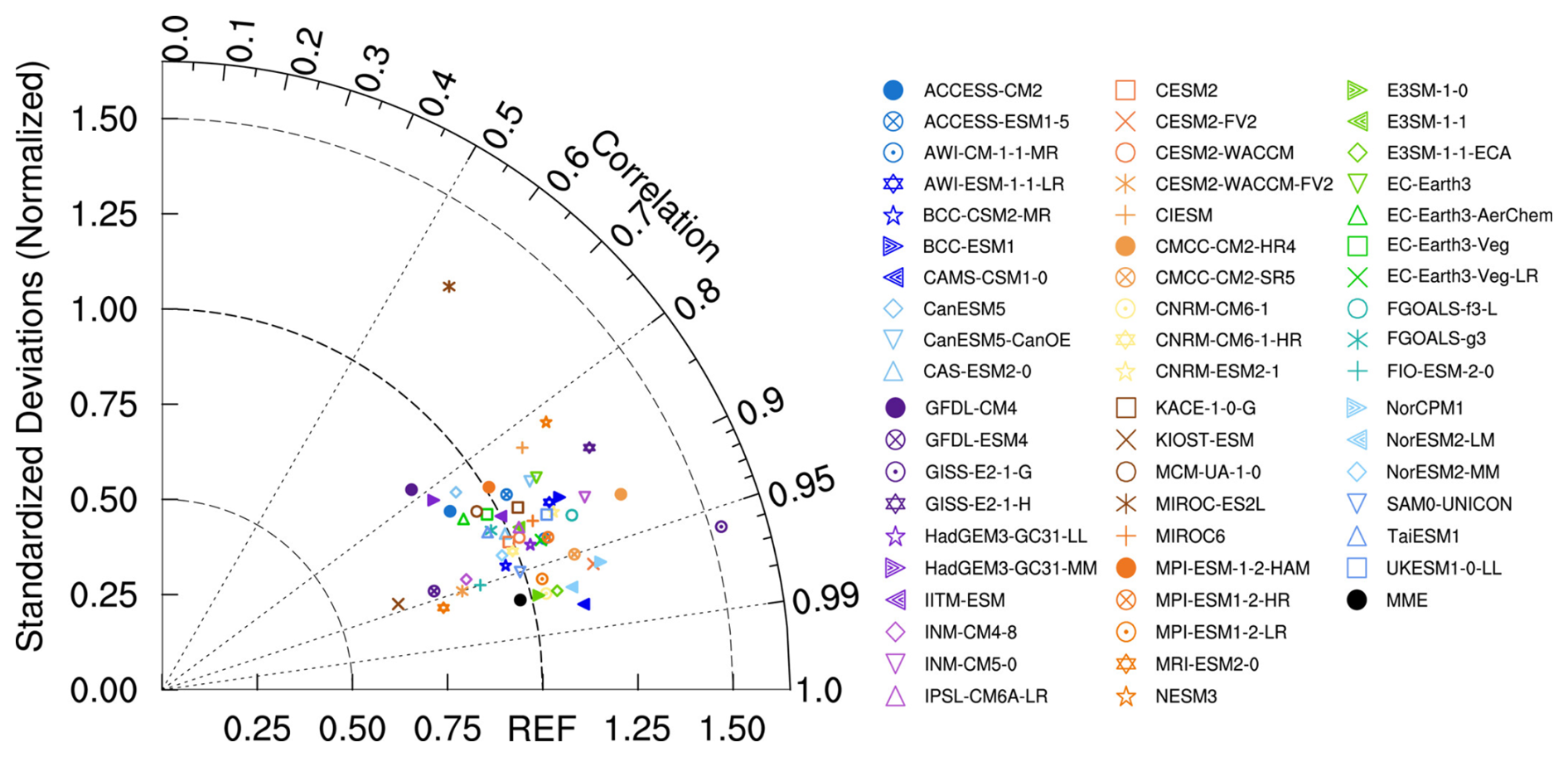
Figure 1 Example for the use of a Taylor diagram showing the geopotential height anomalies at 500 hPa over the Western North Pacific (20–80° N, 120° E–120° W) in individual CMIP6 models, MME and observations, taken from Aru et al. (2023).

A frequent challenge in climate model evaluation is determining whether models yield correct results for incorrect reasons, due to compensating errors (Eyring et al., 2016; Ivanova et al., 2016). There is a possibility that, while a model appears to accurately represent some variable, the underlying processes are not well-captured, which could mask inherent biases in the model. For example, analysing CMIP6 models, Zhao et al. (2022) reported that the cloud radiative effect reveals compensating errors between the modeled total cloud fraction and the liquid water path. These errors offset each other, resulting in a smaller net error in the cloud radiative effect. Di Luca et al. (2020a) addressed the issue of error compensation in CMIP5 simulations of hot temperature extremes by developing a new error metric called the “additive error.” This metric adds up the absolute errors of four components contributing to temperature extremes: the long-term mean, seasonality, diurnal temperature range, and the local temperature anomaly on the day of the extreme. Compared to traditional bias or absolute error metrics, the additive error more sensitively captures the total error in extreme temperature estimates. Furthermore, Di Luca et al. (2020b) defined a new error estimator that aims to minimise error compensation.

It is important to remember that models are calibrated with the aim to reduce anomalies compared to observational data before becoming available in new CMIP generations. During this calibration (often referred to as tuning), parameters, typically associated with unresolved processes such as clouds, convection, or boundary-layer dynamics, are adjusted to improve agreement with observations. Consequently, improvements in overall model performance in new CMIP generations do not necessarily stem from enhanced capabilities in capturing relevant processes, but may instead result from optimized calibration (Knutti, 2010). A related issue is that the same observational datasets used for model calibration are often also employed for model evaluation, which is not optimal as calibration and evaluation datasets ideally should be independent. This concern is even more pronounced when using reanalysis products as reference data, since climate models are an integral part of their generation.

Additionally, observational data can influence model performance through the forcings themselves. For example, in concentration-driven CO2 simulations, observed atmospheric concentrations are prescribed directly for historical simulations, rather than being computed from emissions, as in emission-driven models. This approach further constrains the model output, since the model does not simulate atmospheric CO2 concentrations from emissions via an interactive carbon cycle. Consequently, apparent improvements visible in the model's evaluation do not necessarily indicate a better representation of the carbon cycle itself.

Ideally, the evaluation process also allows insights on how well basic dynamic processes relevant to the research questions are reproduced in models (Knutti et al., 2010b). For a research question regarding rainfall, for example, this could mean to not only analyze the precipitation pattern, but also inspect wind patterns to see if the associated circulation is captured well. Process-oriented model evaluation specifically targets the model performance concerning such dynamics.

2.1.3 Process-oriented Evaluation

This evaluation approach shifts from traditional performance-oriented evaluation to more detailed, process-oriented metrics, which are critical for advancing the next generation of ESMs. Eyring et al. (2005) and Gleckler et al. (2008) emphasise the need to evaluate a wide range of climate processes, since accurately simulating one aspect does not ensure accuracy in others. These authors initiated the development of a comprehensive set of model metrics to assess important processes in climate simulations. Process-oriented evaluation identifies sources and limitations of predictability, guiding model development by revealing deficiencies in the representation of physical processes and thereby enhancing the reliability of climate projections (Eyring et al., 2016). By incorporating process-oriented analysis into diagnostic packages (examples in Sect. 2.5), evaluations become reproducible, accelerating model improvements and establishing benchmarks for progress. As with any standardization effort, however, such benchmarks must be applied with care, as they have the potential to promote model similarity. Another relevant resource in the context of process-oriented evaluation is Simpson et al. (2025), who review the ability of climate models to reproduce historically observed forced trends and outline best practices for confronting modeled and observed signals. Within the MME framework, process-based approaches help identify which processes contribute most to inter-model differences and provide insights into the mechanisms behind model performance. Here, we outline some common use cases and techniques.

Process-oriented diagnostics to reduce model bias: One major focus in the development of process-oriented metrics is the investigation of phenomena with strong bias in the models, as e.g. the Madden-Julian Oscillation (MJO), the dominant mode of tropical intraseasonal variability. To better understand the origins of these biases, a number of diagnostics has been developed to facilitate improvements in the representation of the MJO in weather and climate models (Ahn et al., 2020; Li et al., 2022; Wang et al., 2020). The first process-oriented multi-model comparison study on MJO teleconnections found that biases in simulating the position of the Pacific westerly jets, together with deficiencies in MJO representation, contribute substantially to errors in MJO teleconnections (Ahn et al., 2017; Henderson et al., 2017). Similar efforts exist for the El Niño–Southern Oscillation (ENSO), for which Planton et al. (2021) provide a dedicated metrics package.

Improving projections by process-oriented multiple diagnostic ensemble regression: Karpechko et al. (2013) developed the multiple diagnostic ensemble regression (MDER) method that constrains climate projections using observed diagnostics, applying it to Antarctic ozone columns. By identifying key processes that influence ozone, MDER explains a substantial fraction of the inter-model spread in projected ozone across climate chemistry models and outperforms the unweighted multi-model mean in pseudo-realistic validation. Building on this approach, Wenzel et al. (2016) applied the MDER algorithm, implemented as a diagnostic in ESMValTool (see Sect. 2.5), to analyze projections of the austral jet position under the RCP4.5 scenario in CMIP5 simulations. They found that MDER reduces uncertainty in the ensemble-mean projection without substantially altering the long-term mean position of the jet.

Identifying the role of model configurations: Another significant aspect of process-oriented model evaluation is understanding how specific characteristics are influenced by model configurations, such as resolution and parameterization schemes. Kim et al. (2018) proposed a set of diagnostics to assess how model physics affect the representation of tropical cyclones, particularly their intensity in GCMs. The findings suggest that model-specific factors, beyond large-scale environmental parameters, play a key role in shaping tropical cyclones' intensity, with differences in convection schemes contributing significantly to the inter-model spread. Wing et al. (2019) and Moon et al. (2020) further applied these methods, with Moon et al. (2020) showing that tropical cyclone wind structures are strongly influenced by model resolution. Accordingly, Dirkes et al. (2023) emphasizes the necessity of applying the developed diagnostics for tropical cyclone analysis in CMIP6 models.

Using idealization or a hierarchy of models: Another approach is to design model configurations that isolate individual processes and components, allowing to test their relevance for specific phenomena. For example, Katzenberger et al. (2024) employed an aquaplanet configuration with a circumglobal land stripe to evaluate the meridional circulation, particularly the Hadley cell, in an idealized setup. By shifting the landstripe north and southwards, and by modifying the surface albedo or aerosol concentrations, the role of these features in shaping monsoon dynamics could be systematically isolated. More generally, iteratively adding components and increasing the complexity and realism of the setup within a hierarchy of models enables the isolation of individual processes and the assessment of their contributions to the overall model performance. See also e.g. Zhou and Xie (2018) for more insights to this approach.

Using causal inference: In Section 4.1, we provide insights into how ML techniques can be applied to improve process-based evaluation by identifying causal relationships.

Another example of process-oriented assessment is provided by Fasullo et al. (2020), who present a thorough analysis of CMIP representation of the leading Earth system modes of variability. Additional applications include regime-based evaluation approaches of low-level marine clouds, where distinguishing stratocumulus from shallow cumulus regimes has helped diagnose persistent cloud-cover and radiative biases in CMIP6 and CMIP5 models and inform targeted model improvements (Črnivec et al., 2023; Cesana et al., 2023). Process-based analyses have also demonstrated that the ENSO–Indian Summer Monsoon teleconnection is robustly represented in CMIP5 and CMIP6 models, consistent with a realistic simulation of the coupled Hadley–Walker circulation and associated precipitation responses (Roy and Tedeschi, 2016; Roy et al., 2017; Fasullo et al., 2020). We provide further details and examples of process-oriented analyses in the Supplement S3.

2.2 Model Dependence

ESMs are developed by multiple modelling groups worldwide. Ideally, the models in a MME would be independent, thereby providing an adequate representation of the epistemic uncertainty. Historically, climate projections are derived by calculating simple averages across the MME, based on the assumption that the ensemble mean offers the most accurate representation of the Earth system by synthesizing the collective modelling efforts (Abramowitz et al., 2019; Knutti et al., 2010a). Assuming independence implies that the MME reflects a sufficiently broad range of uncertainties, and the averaging smooths out individual model biases. In practice, however, the development of ESMs is often not independent (Pincus et al., 2008).

Components that address modelling challenges or have demonstrated strong performance are often shared among multiple ESMs, including e.g. the dynamical core for resolving grid-scale dynamics or components addressing sub-grid-scale phenomena (e.g., parameterization schemes). For example, the McICA radiation scheme (Pincus et al., 2003) provides an efficient and flexible representation of one-dimensional radiative transfer in a cloudy atmosphere, and is thus implemented in multiple ESMs such as several US models (NSF NCAR CESM2, NOAA GFDL-CM4, DOE E3SM-1-0), the Canadian model (CanESM5), the UK model (HadGEM3), and the Norwegian model (NorESM2). Similarly, the NEMO ocean model is widely used across modelling centers, including e.g. HadGEM3 and NorESM2, further underscoring the sharing of model components. Figure 2 illustrates the shared model history tracing back to a few AGCMs (Kuma et al., 2023).

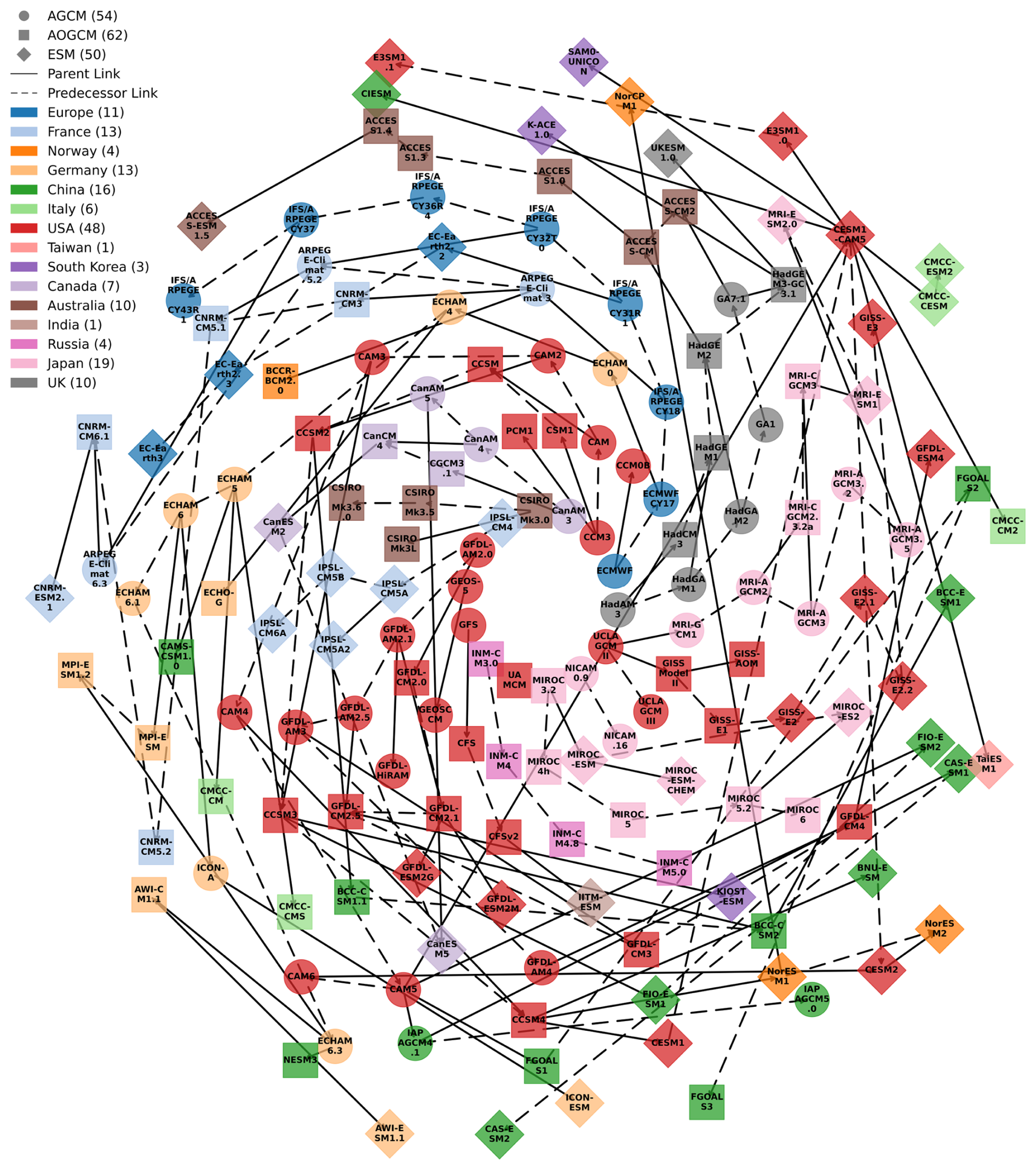
Figure 2 Spiral plot of climate model dependencies, adapted from Kuma et al. (2023). The oldest model in any given family is in the center of the plot, spiralling out as more models are made. Model type is differentiated by shape of marker, and link type is differentiated by arrow type (solid for parent or dashed for predecessor). Models developed in different countries are assigned distinct colors. Markers indicate atmosphere general circulation models (AGCMs), atmosphere-ocean global circulation models (AOGCMs), and Earth system models (ESMs). Numbers of models from each country are indicated in brackets in the legend. ECMWF models are denoted by the country “Europe”.

In addition to dependencies between modelling groups, individual centers often contribute multiple closely related model configurations, for example differing in horizontal resolution (e.g., MPI-ESM1.2-HR for high resolution versus MPI-ESM1.2-LR for low resolution) or in the inclusion of additional components, such as interactive vegetation in EC-Earth3-Veg compared to EC-Earth3. If such dependencies are not accounted for and all models are included with equal weight in a multi-model mean, modelling centers that provide several related configurations effectively receive greater weight than others. This issue is particularly relevant in multi-model studies with a limited number of included models.

Diverse analyses confirm that the number of independent models in CMIP is smaller than the total number of participating models (Jun et al., 2008; Masson and Knutti, 2011; Pennell and Reichler, 2011). Because errors across different models are often being correlated (Knutti et al., 2010a), the lack of independence can lead to amplified biases (Jun et al., 2008; Knutti, 2008; Reichler and Kim, 2008; Tebaldi and Knutti, 2007). Moreover, apparent convergence among model results and the associated reduction in ensemble uncertainty may be mistakenly interpreted as strong agreement between models, when in fact they arise from structural dependencies.

The lack of a universally accepted and unambiguous definition of model independence complicates efforts to systematically account for model dependence in MME studies. Some definitions focus on the conceptual idea of whether or not a model adds novel additional information to the MME (Masson and Knutti, 2011). Others adopt a more analytical approach to understanding model dependence, offering examples for evaluating model dependence and using their framework (e.g., Annan and Hargreaves, 2017). Despite such advances, no broadly accepted solution has yet emerged. Further approaches, such as weighting schemes (Sect. 2.3) have been proposed, but these tend to be problem-specific and struggle to capture the full complexity of model dependencies. The metadata reporting requirements introduced in CMIP6 have made comprehensive assessments of model dependence possible, thereby representing a meaningful advance in transparency. As new model generations are developed and incorporated to CMIP, continued efforts to quantify and correct for model dependence will be essential to ensure robust ensemble projections that reflect true uncertainty.

2.3 Model Selection and Weighting Methods

CMIP MME weighting and selection techniques are used to categorize the CMIP models based on historical model performance (see Sect. 2.1) and independence (see Sect. 2.2) using several metrics (Palmer et al., 2023), which is crucial for optimizing accuracy and reliability in projections (Strobach and Bel, 2020). Several performance-based and statistical approaches are used for MME weighting (Bhowmik and Sankarasubramanian, 2020; Brunner et al., 2020). Performance-based weighting assigns weights based on the ability to reproduce observed historical climate patterns, while statistical model weighting assigns weights based on properties like independence and spread (Brunner et al., 2020). Both approaches are discussed in this section, complemented by subselection approaches. Model weighting and subselecting to account for model outliers is discussed specifically in Sect. 3.3. It is also important to note that some studies may be primarily interested in assessing the overall performance of the full CMIP ensemble. Applying weighting or model subselection is not relevant to such analyses.

2.3.1 Accounting for Model Performance

Most studies in the literature use simple multi-model means, thus equally weighted MMEs to project future climate change impacts (Shuaifeng and Xiaodong, 2022). While such approaches capture the overall trends across all models, equal weighting without any model selection has been criticized for not considering model performance (Shin et al., 2020). Incorporating information on model skill – by emphasizing better-performing models and down-weighting or excluding models with poor simulation capabilities – can improve both the accuracy of projections and the assessment of uncertainty in CMIP MMEs (Merrifield et al., 2020).

Weighting, however, is a challenging process as the basis for weights must be determined and other not yet identified but equally relevant factors may be neglected. Moreover, the relevance of specific model features for a given phenomenon may change under future climate conditions, making it questionable to assign weights solely based on present-day performance, as discussed previously in the context of model evaluation. In addition, weighting schemes may inadvertently favor structurally similar models that produce “mainstream” results, while penalizing outlier models that could provide valuable insights (see also Sect. 3.3). When bias correction is applied, assessing model performance becomes particularly challenging, as differences between models and observations are largely removed, complicating performance-based weighting. Shin et al. (2020) addressed this issue by proposing a hybrid weighting approach that preserves performance information while avoiding unrealistically extreme model weights.

Despite these challenges, several studies have demonstrated the potential benefits of performance-based model weighting for climate projections. Tang et al. (2021) found that weighted MMEs produce more robust projections of extreme precipitation over the Indo-China Peninsula and southern China than unweighted ensembles. Similarly, Shuaifeng and Xiaodong (2022) applied a rank-based weighting approach to CMIP6 MMEs for projecting and quantifying uncertainty in cold surges over northern China. Brunner et al. (2020) discovered a reduction in the projected warming when applying model weighting because some models showing high future warming have systematically lower performance skills.

Another approach to account for model performance is the selection of a subset of models. This can also be considered as a weighting method, which uses the weight 1 for included models, and the weight 0 for excluded models. MMEs with optimized sub-selection can reduce the computational load and have been shown to decrease the ensemble-mean RMSE, e.g. by roughly 10 %–20 % for air temperature and approximately 12 % for precipitation relative to the full multi-model mean (Hamed et al., 2021; Herger et al., 2018; Snyder et al., 2024). The central challenges in subselecting are the identification of performance metrics, as already discussed in Sect. 2.1, as well as the definition of selection criteria that should be made transparent. Herger et al. (2018) compared different sub-selection approaches, including random ensembles, performance-based ranking, and optimal ensemble subselection, and found improved performance over the multi-model mean in some cases. In a random ensemble, multiple models are combined randomly without an explicit optimization strategy. In performance ranking, models are ranked based on metrics such as accuracy, Q-statistics, mean square error etc. In optimal ensemble sub-selection, a subset of models is chosen that maximizes performance. Almazroui et al. (2017) similarly found that a subset of the best-performing models showed better temperature and precipitation projections over the Arabian Peninsula. Numerous further examples exist, e.g. including the ENSO teleconnection (Roy et al., 2018) and lightning over South/South-east Asia (Chandra et al., 2022).

2.3.2 Accounting for Model Dependence

As discussed in Sect. 2.2, climate models are not fully independent. A common approach to address this issue is by weighting models based on their independence from others. Sanderson et al. (2015) developed a mathematical formulation to quantify model uniqueness and assign corresponding weights. Boé (2018) argues that model interdependencies are more effectively assessed through code similarity instead of through result similarity. Although evaluating source code similarity is indeed challenging (due to issues such as the complexity of model architectures, differing programming languages, licensing issues and proprietary restrictions), it has the potential to reveal shared model components and algorithms that may not be evident from model output comparisons alone. Recent model selection approaches also emphasize model independence (Snyder et al., 2024), with tools such as ClimSIPS explicitly accounting for model dependence (Merrifield et al., 2023). Assessing both source-code similarity and similarity in model results enables the identification of shared methodologies that can lead to correlated predictions, thereby highlighting potential redundancies within MMEs that may bias ensemble statistics. Integrating these measures into weighting schemes can therefore improve the robustness of MMEs and contribute to more reliable and less biased projections.

2.3.3 Combined accounting for Model Performance and Dependence

Knutti et al. (2017) proposed a model weighting method that accounts for model performance as well as model dependency. This method includes two distance metrics, from models to observations, and among models. Here the “effective repetition of a model” within an ensemble, outlined by Sanderson et al. (2015), is accounted for, along with the accuracy of a model with respect to observations.

2.4 Uncertainty Characterization

Model selection and weighting ideally improves uncertainty which remains inevitable when trying to predict climate (Knutti et al., 2019). Characterizing and understanding it is essential for guiding model evaluation and development, for science and risk communication, and for assessing climate impacts (Deser et al., 2012a; Deser, 2020; Snyder et al., 2024). When using future projections from CMIP, three types of uncertainty must be dealt with (Hawkins and Sutton, 2009; Lehner et al., 2020; Simpson et al., 2021): scenario or forcing uncertainty, natural variability uncertainty, and model uncertainty. The scenario uncertainty arises because it is not known how human emissions of greenhouse gases and other pollutants from all over the world will develop in the future, and it is accounted for by modelling different emission scenarios (O'Neill et al., 2014; van Vuuren et al., 2025). Natural or internal variability uncertainty is due to the chaotic and, thus, unpredictable evolution of the climate system (Deser et al., 2012b), having a great impact on climate projections (Lehner and Deser, 2023). The unique realization of our future climate is the response to the combined effect of anthropogenic forcing and internal Earth system variability. Although internal variability uncertainty cannot be reduced, it is quantifiable (Deser, 2020), and using large ensembles of a single model is helpful for this purpose (Tebaldi et al., 2021). Finally, the third type – model uncertainty – results from our imperfect attempts to predict the aforementioned real world realization. It includes differences among models as well as the varying results that can be obtained within the same model when varying its parameters. While model uncertainty can be reduced, its interpretation and quantification depend strongly on how the ensemble is constructed (Knutti et al., 2019). An adequate understanding of uncertainty has the potential to help MMEs users with model selection and thereby reduce computational burdens (Snyder et al., 2024).

Decomposing the total uncertainty of climate estimates into contributions from scenario, internal, and model uncertainty provides insights into projections' reliability and potential for reducing uncertainty. This process is called uncertainty partitioning, and it often involves quantifying the consistency among different members of a MME (Hawkins and Sutton, 2009; Lehner et al., 2020; Woldemeskel et al., 2012; Yip et al., 2011). For long-term means of climate data, Hawkins and Sutton (2009) proposed a widely used method for uncertainty partitioning: they fit a polynomial to each model's output in the time dimension to separate the forced response from the internal variability. The variance across different model's polynomials corresponds to the model uncertainty, and the mean of the different residuals across models represents the internal variability. Finally, the scenario uncertainty is the variance across multi-model means for different forcings. This method assumes (i) that the forced response can be approximated by the polynomial and (ii) that the arithmetic sum of the different uncertainties comprises the total uncertainty.

To consider the potential non-additive nature of the total uncertainty (ii), Yip et al. (2011) used analysis of variance (ANOVA) – an approach that partitions the total variance into components due to different sources of variation – to improve the uncertainty partitioning. Woldemeskel et al. (2012) expanded the uncertainty quantification methodology to include also the spatial dimension, by introducing the Square Root Error Variance (SREV) method. This method has proven useful for highlighting regional differences in uncertainty. More recently, exploiting the increasing computational capabilities, Lehner et al. (2020) overcame the assumption of the polynomial fit (i) from Hawkins and Sutton (2009), which produced significant regional biases, by using several SMILEs. Instead of calculating the variance of the polynomials as in Hawkins and Sutton (2009), in this approach, the model uncertainty is calculated as the variance across ensemble means from the available SMILEs. This reduces methodological assumptions and thereby improves the results, making SMILEs currently a broadly used tool to partition uncertainty in climate projections. It is important to note that the lack of independence between models (Sect. 2.2), and the methods to account for it (Sect. 2.3) must also be considered in this context.

A question that should be considered, although it can only be partially answered, is whether the MME spread is realistic, too narrow or too broad. The uncertainty may be too broad if observations are not used correctly to tune models, or if the models have extensive and diverse structural errors. The ensemble may be too narrow, and thus overly confident if the models are structurally very similar, if they are overfitted to observations or if uncertain processes are missing. It is also important to recognize that present-day and future uncertainties arise from different sources: present-day uncertainty mainly reflects the models' ability to reproduce observations, whereas future uncertainty stems from variations in how models represent physical processes and feedbacks (Sanderson and Knutti, 2012). Care should be taken when assuming that the spread of present-day or historical simulations will be the same in the future.

As discussed in Subection 2.1, relying solely on how well a model reproduces past climate to assign confidence can be misleading: models that perform well historically may not accurately project future climate changes, while models that perform poorly may still provide useful information about future conditions (Hall et al., 2019). An evaluation and uncertainty reduction technique that avoids this bias is the development of emergent constraints (Hall et al., 2019). An emergent constraint refers to a statistically robust relationship across a MME between an observable present-day quantity (x) and a projected future change in a quantity (Δy), typically approximated as linear (Simpson et al., 2021). When this relationship is robust, observations of x can be used to constrain the plausible range of y, thereby reducing uncertainty. This is commonly achieved by analyzing the probability distribution function of y conditioned on the observed value of x. This method has been used for assessing the uncertainty of many processes within different Earth system components (Keenan et al., 2023; Nijsse et al., 2020; Shaw et al., 2024; Simpson et al., 2021; Smith et al., 2022; Thackeray et al., 2022). ML approaches have also been used to demonstrate a potential to discover and explore emergent constraints (Nowack et al., 2020). Despite the usefulness of emergent constraints, care should also be taken when interpreting the results, since the method assumptions may produce overconfident predictions and may be vulnerable to artifacts within the model (Breul et al., 2023; Sanderson et al., 2021), similar to other uncertainty reduction methods.

While climate models exhibit high confidence in thermodynamic aspects of climate change (e.g. global temperature increase) due to robust theoretical and observational evidence, dynamic aspects, particularly related to atmospheric circulation, present significant uncertainties due to their nonlinearity and feedbacks (Shepherd, 2014). Model uncertainties in these two components are uncorrelated (Zappa and Shepherd, 2017), meaning that errors in one component do not influence or predict the errors in the other, so separating them allows better understanding of where the biggest uncertainties lie.

2.5 Available Tools for MME Analysis

The analysis of CMIP datasets is greatly facilitated by a variety of tools developed within the global climate science community. However, the wide range of available tools was not centrally cataloged, making it difficult to obtain a clear overview of available tools and their capabilities. To address this gap, the WCRP CMIP has undertaken an effort to compile a central repository (https://wcrp-cmip.org/tools/, last access: 14 April 2026) that encompasses a broad range of resources.

The repository includes data access platforms (e.g., Earth System Grid Federation, Climate Data Store, IPCC data distribution centre, PANGEO, CAVA, Climate Information Portal), which facilitate accessing large and complex data volumes. It also lists widely used command line operators (e.g., ncview, NCO, CDO) and programming languages suitable for climate data analysis (such as Python, R, Julia), together with useful packages (e.g., multiple Python packages such as matplotlib, scipy, pandas, Iris, xarray, xGCM, xMIP, xclim, xCDAT, UXarray, Metpy, aospy). In addition, the repository contains several comprehensive evaluation and benchmarking tools, such as ESMValTool, bgcval2, RUBISCO, PCMDI Metrics Package, AMBER, and the MDTF Diagnostic Package. These evaluation tools include diagnostics designed to address specific scientific questions. For example, ESMValTool incorporates the Climate Variability Diagnostics Package (CVDP, Eyring et al., 2020; Phillips et al., 2020, 2014; https://github.com/NCAR/CVDP-ncl, last access: 14 April 2026), which facilitates the analysis of modes of climate variability and change in models and observations (Maher et al., 2024). Another important initiative in process-oriented evaluation is led by the Model Diagnostics Task Force (MDTF) under NOAA's Climate Program Office (CPO) Modeling, Analysis, Predictions, and Projections (MAPP) program. It promotes the development and use of process-oriented diagnostics (see Sect. 2.1) in climate and weather prediction models (Maloney et al., 2019; Neelin et al., 2023). Additionally, the WCRP repository includes various data analysis and visualization tools, including the IPCC WGI Interactive Atlas, Panoply, TempestExtremes, CAVA, TECA, KNMI Climate Explorer, and Google Earth Engine. Figure 3 highlights some of these tools, aiming to promote their use across the wider climate community. Basic information about each tool is provided by “Tools description cards” on the CMIP website, which include links to tool websites, documentation, tutorials and community support resources. Finally, it should be emphasized that the tools repository is actively maintained and continuously updated. To further enhance its utility for the broader climate science community, new contributions are highly welcome.

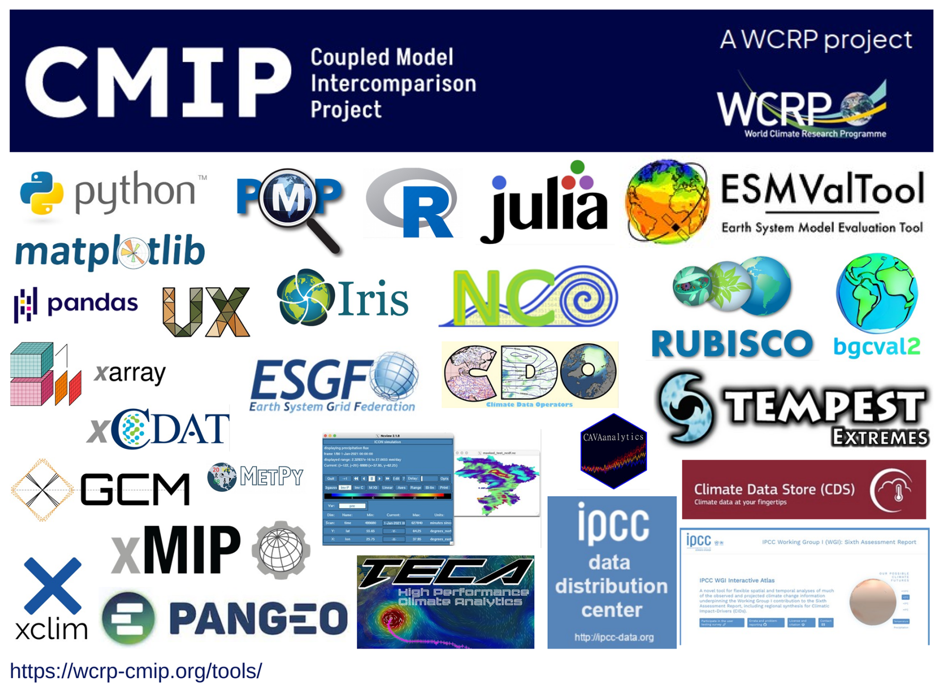
Figure 3 Collection of useful tools for using climate data available at https://wcrp-cmip.org/tools/ (last access: 14 April 2026).

While the CMIP tool repository is a key resource for many widely used climate analysis tools, it does not cover all available resources. The wider open-source ecosystem – especially within the Python community – offers many additional tools and libraries for climate data analysis and is supported by a large and active scientific community on platforms such as GitHub.

3 Complementing Topics and Challenges

Building on the general workflow involved in MME studies in Sect. 2, we draw on the experience within the Fresh Eyes community to identify common topics and challenges that arise in this context. All of these aspects are also relevant to the subsections in Sect. 2; however, our aim here is to provide a dedicated overview of specific topics, allowing researchers to access the most relevant information in one place.

3.1 Number of Models

Any MME analysis has to face the question of how many models to include, which is not straightforward, as it involves the trade-offs between model diversity, computational cost, and the accuracy of the results. Increasing the number of ensemble members has the potential to enhance the robustness of the results by reducing statistical uncertainty. At the same time, state-of-the-art climate models remain computationally expensive. Downloading and processing these large datasets, particularly in the context of major intercomparison projects like CMIP, is also a resource-intensive challenge that limits the number of models included in MME studies. These challenges raise the question how many models are actually required to form a “good” ensemble size. Here, we focus on the number of models within a MME. A closely related question exists in the context of large ensembles where the number of perturbed simulations is discussed. Some examples for the number of simulations in large ensembles are provided in Sect. 4.2. However, many of the arguments and findings in this section apply for both contexts.

3.1.1 Lower threshold of ensemble size: At least 5 models

If the ensemble size is too small, the inter-model may not be fully captured. This has the potential to lead to an underestimation of uncertainties and can consequently result in an overestimation of the models' performance and thus an overconfident interpretation of the results. It is even possible that a too small ensemble size leads to qualitatively different findings, as shown by Milinski et al. (2020). In this study, the subsets of two and three models showed a warming after a volcanic eruption, while the actual known response would be cooling. So, how many models or simulations should be used as a minimum? Several studies have shown that the error (e.g. root mean squared error when compared to reference data) is reduced substantially up to about five models in different contexts (Herger et al., 2018; Knutti et al., 2010a; Mendlik and Gobiet, 2016; Milinski et al., 2020; Steinman et al., 2015). Adding further models is generally beneficial, but the improvement per additional model is much smaller. Mendlik and Gobiet (2016) find that the subset size can be reduced from 25 to 5 while still being representative for the entire ensemble. As these studies refer to different quantities and research questions, and were conducted independently, but still share five as a lower “threshold”, we propose five models/simulations as an initial baseline minimum for MME studies. Depending on the research question however, the minimum number of required models might vary. It can be determined by a specific method, as explained below.

3.1.2 Determining individual minimum ensemble size

If feasible, determining the appropriate minimum ensemble size on a case-by-case basis – depending on the specific research question and requirements – is preferable to adopting a general minimum. Milinski et al. (2020) proposed a procedure applicable to diverse research questions. After (1) defining the research question, (2) an error metric (e.g. RMSE) as well as a maximum acceptable error has to be decided. Then (3), the error for randomly sampled subsets of different sizes has to be quantified. The number of required models can now be identified as the smallest subset size that has an error below the chosen threshold (4). If the identified model number is less than half of the initial sample (e.g. the identified subset included 40, thus less than 50 members, when evaluating 100 members) the estimated subset size is robust (5). This requirement is introduced to avoid resampling bias, as random subsets close to the full ensemble share many members, are no longer independent, and therefore tend to reproduce the full-ensemble signal by construction rather than providing an unbiased estimate of the required ensemble size, see Milinski et al. (2020) for details. While this method provides a straight-forward method to identify the ideal minimum number of models in an ensemble, it requires the availability and analysis of a high number of model simulations. Consequently, this method might not be feasible for all studies.

3.1.3 Remarks for including more models

While the considerations above address the identification of a minimum ensemble size, additional models have the potential to further improve the model performance. For some applications, larger ensemble sizes are even required, e.g. for the quantification of internal variability, as estimating higher-order moments of the distribution demands a sufficiently large ensemble (Milinski et al., 2020). Generally, adding further models improves the statistical robustness of the MME analysis, but it has to be remembered that the added models should at least partly be independent of the existing models as otherwise only the weight of single models is increased without any physical reason (Knutti, 2010). See Sect. 2.2 for more details. A too large ensemble size has also the potential to increase the spread beyond a realistic range as the inclusion of outliers becomes more probable (Knutti, 2010). Section 3.3 therefore discusses strategies for identifying and handling outliers in more detail. Another consideration becomes relevant when working with different scenarios. As the range of uncertainty increases with the number of models, using the same number of models across all scenarios is essential to ensure comparability (Knutti et al., 2010a).

3.2 Extremes

Extreme weather and climate events have significant impacts on human society and ecosystems. Understanding the drivers and producing reliable future projections of these low-frequency high-impact events is therefore essential for effective climate change adaptation planning. When using MMEs to study extreme climate events, ensembles offer both strengths and challenges.

MMEs based on CMIP or CORDEX are widely used both in regional and global studies concerning climate extremes (Kim et al., 2020; Soares et al., 2023; Vogel et al., 2020; Yang et al., 2012). These studies typically apply statistical approaches, such as probabilistic modelling, and/or using climate extremes indices defined by the Expert Team on Climate Change Detection and Indices (ETCCDI). Extreme Value Theory (EVT) provides the theoretical foundation for analyzing extreme events by offering statistical methods to model the tails of probability distributions (Coles, 2001; DelSole and Tippett, 2022). One widely used approach within EVT is Generalized Extreme Value (GEV) distribution analysis (Rypkema and Tuljapurkar, 2021), a statistical framework for modelling the tail of the distribution of rare events. For example, GEV analysis is frequently used to estimate return periods of extreme rainfall events, allowing assessment of how the frequency and intensity of such events may change under future climate scenarios (Wehner, 2020). By fitting GEV to observed and modeled data, researchers can evaluate shifts in extreme event characteristics.

A major advantage of using the mean of the MME is that averaging across models reduces noise from internal variability and thereby amplifies the climate change signal. This can also help identify trends in extreme events (IPCC, 2021). However, the MME mean might not always be the best choice, particularly when examining the intensity and frequency of extreme events (Knutti et al., 2010b). Using MME's median or mean can sometimes mask the severity of local extremes, as averaging across multiple ensemble members can obscure the range of possible outcomes of individual extreme events. This is especially the case when some models predict significantly different extreme event trends, potentially leading to an underestimation of risks. Uncertainty remains for both hot and cold extremes, with some models deviating considerably from the multi-model mean. Uncertainties are particularly large for precipitation extremes, where, despite a general tendency toward heavier precipitation and longer dry periods, several models project opposing trends in specific regions (Sillmann et al., 2013).

In studies on climate extremes, it is therefore important to evaluate how well each model performs in simulating extremes (Kim et al., 2020; Sillmann et al., 2013) and to correct for biases when appropriate. However, as discussed in Sect. 2.1, model evaluation is conducted using performance-oriented or process-oriented approaches that generally tend to focus on the models' ability to capture mean climate states or large-scale circulation patterns rather than models' extreme event representation. Dedicated evaluations tailored to extremes are therefore required, capturing relevant temporal resolution, region and variables and comparing to an appropriate reference data set. For example, Kim et al. (2020) evaluated the CMIP6 MME against ETCCDI climate indices and identified systematic biases, such as a persistent cold bias in cold extremes over high-latitude regions. When comparing CMIP6 models with CMIP5, they found only limited improvements in simulating temperature and precipitation extremes, highlighting the need for further advancements in the understanding and representation of extreme climate events in ESMs. As a step following the evaluation, employing model weighting is one possible approach to address shortcomings, enhancing the accuracy and reliability of extreme event projections (Balhane et al., 2022).

When studying extreme climate events, uncertainty is another aspect that is important to account for. As discussed in Sect. 3.1, ensemble size strongly influences uncertainty estimates, with larger ensembles allowing a more complete sampling of the range of possible outcomes. In practice, many studies of climate extremes using MMEs rely on a single ensemble member per model to ensure comparability across models (Kim et al., 2020). However, using only one ensemble member per model could miss some of the variability in extreme events that larger ensemble runs could capture, particularly as often not too extreme members are submitted for intercomparison projects as CMIP. Nevertheless, given the constraints on computational resources and the availability of large ensembles, this method remains a common compromise.

While increasing ensemble size can help reduce uncertainties, it does not eliminate the limitations inherent to individual models. Downscaling techniques, either statistical or dynamical using RCMs, can provide higher-resolution data to improve the representation of extremes in specific regions. For example, the bias-adjusted high-resolution RCM outputs in the EURO-CORDEX project showed an improvement in the simulation of extreme temperature and precipitation indices across Europe, underscoring the value of RCMs for more reliable and region-specific climate projections (Coppola et al., 2021; Dosio, 2016). MMEs based on RCM projections are particularly valuable for highly vulnerable regions, offering insights into potential changes in local extreme events (Dosio, 2017; Tegegne et al., 2021) and supporting planning for challenges such as water scarcity, food security, and disaster preparedness. For more details regarding downscaling, see also Sect. 3.4.

3.3 Outliers

Outlier models have at times been disregarded in MME analyses because convergence toward the ensemble mean has been interpreted as a measure of model reliability. However, the use of convergence as a measure of model reliability has been criticized because it favors simulations that are closer to the multi-model mean, while underrepresenting uncertainty across a wider range of plausible outcomes (Tebaldi and Knutti, 2007). For example, the original version of the reliability ensemble average (REA) weighting method assigns higher weights to models that better reproduce the current climate, but also penalizes models that diverge from the ensemble mean (Giorgi and Mearns, 2002). As a result, outliers receive lower weights even when their differences may reflect physically plausible behavior rather than poor model performance. This is especially problematic because convergence toward the ensemble mean can partly arise from genealogical similarities among models, rather than independent confirmation of a result (Tebaldi and Knutti, 2007). Despite these concerns, there is a history of privileging convergence towards the MME mean within the climate science community. For example, in the third IPCC assessment report two models were discarded because of extreme warming projections associated with very high climate sensitivity (Tebaldi and Knutti, 2007). More recently, convergence-based ideas continue to influence MME subsetting approaches (Palmer et al., 2023) and are still used, at least in part, in MME evaluation frameworks (Amali et al., 2024). Whether emphasizing convergence is appropriate depends on the purpose of a given study. For applications such as the analysis of climate extremes, averaging across models can mask the full range of possible outcomes. In these cases, outlier models may provide valuable information about plausible high-impact scenarios rather than representing spurious deviations from the ensemble mean. See also Sect. 3.2 for more details on extremes in MMEs. Building on the insights on weighting and building subsets of models in Sect. 2.3, we discuss here in more detail how and when to account for outliers.

3.3.1 Exclusion of Outliers

One approach to account for outliers, is exclusion, meaning the removal of models with outlier status from an ensemble. While this can help reduce unrealistic spread and improve agreement with observations, it carries the risk of omitting simulations that represent rare but physically plausible events. In some cases, however, the benefits of exclusion outweigh the drawbacks. For example, Mudryk et al. (2020) identified outlier models for some seasons and regions in their study of snow cover change in the Northern hemisphere. These models, which overestimated snow cover in areas of low snow mass, were excluded to improve the alignment between observational data and CMIP6 MME projections. Similarly, the Swiss Climate Scenarios CH2018, based on EURO-CORDEX, excluded some outlier GCMs to narrow uncertainty ranges for temperature and precipitation (Sørland et al., 2020). The consequences of outlier inclusion or exclusion have been explored in the literature. Sun and Archibald (2021) compared “aggressive” and “conservative” approaches – respectively including and excluding outliers – and found that, for their study, the differences in results were relatively minor. Similarly, Bracegirdle and Stephenson (2012) presented analyses both with and without outliers to illustrate the sensitivity of polar warming estimates to outlier inclusion and different forms of regression. Overall, while models with outlier projections may be excluded to improve MME alignment with observations or to reduce uncertainty, this should be done with caution. Exclusion is most justified when a model is known to be deeply flawed. Otherwise, removing projections of rare but plausible events may limit the assessment of adaptation strategies and risk management options (Knutti, 2010).

3.3.2 Weighting or Penalization

MME inclusion of outlier models is often accomplished through weighting. One commonly used approach is weighting based on root-mean-square error (RMSE) skill scores. For example, Tegegne et al. (2020) preserve MME spread by applying the Katsavounidis–Kuo–Zhang algorithm to select ensemble members based on their contribution to representing the full range of variability within the sampling space for extreme indices of interest, as recommended by World Meteorological Organization's ETCCDI. The IPCC characterizes this approach as suitable for detecting “moderate extremes”–events expected to occur up to 10 % of the time (Seneviratne et al., 2012). In this approach, detecting extremes prior to taking the MME mean is useful for weighting members such that the full range of variability within the MME is largely preserved. To identify and characterize more extreme events, methods based on extreme value theory (EVT) are required. EVT focuses on values located in the very ends of tails of probability distribution functions (PDFs) and is therefore better suited to representing rare, high-impact extremes (DelSole and Tippett, 2022).

Among weighting methods rooted in classical statistics is the use of outlier insensitive methods. These are methods that retain outlier models while limiting their influence on the ensemble result. Such methods include using the ensemble median instead of its mean as a measure of the MME's center which reduces sensitivity to outliers (Ge et al., 2021). Rank based tests of statistical significance provide another option. Because they rely on the rank, or position of a value within a PDF, rather than the value of a particular data point within a sample, these are largely insensitive to outliers (DelSole and Tippett, 2022). This test is recommended by the World Meteorological Organization for hydrological data analysis and is robust to outliers and non-normal data distributions (Rojpratak and Supharatid, 2022).

Weighting methods based on Bayesian statistics have been developed to sample uncertainty across a broad statistical space. Compared to the frequentist statistics which uses a fixed population parameter to describe probability distributions, Bayesian statistics uses a conditional parameter that depends on the shape of the PDF for a given dataset (Clyde et al., 2022). Xu et al. (2019) apply Bayesian model weighting to statistically downscale precipitation data for site-specific analyses. The authors argue for the use of statistical downscaling due to its relatively low computational expense with finer spatial and temporal resolution data. At the same time, they note that dynamic downscaling can underestimate extremes and be overly sensitive to outliers. These limitations are addressed by applying a Bayesian weighted average, which reduces outlier influence while retaining information about uncertainty.

Penalization refers to methods that are explicitly designed to reduce the weight of outlier models within an MME. This can be achieved through bias correction and ridge regularization. In Shin et al. (2020) outlier models are defined as those that generate projections that are unusually close to the hydrological variable in observation data, which the authors attribute to excessive regional calibration to observations. To limit the influence of such models, they propose a hybrid method combining Bayesian weighting with bias correction. Ridge regularization, frequently used in ML contexts, is a form of linear regression that incorporates a penalty term to constrain variables with unusually strong linear correlations, thereby reducing the risk of overfitting. Labe and Barnes (2022) apply ridge regularization to limit the sensitivity of an artificial neural network to outlier influence.

3.4 Downscaling Techniques

Acquiring regional information on climate change is essential for impact, vulnerability, and adaptation studies. While CMIP GCMs are internationally established sources for climate projection data, their typical grid resolution of 100–250 km (Liang-Liang et al., 2022; Weigel et al., 2010) limits the ability to provide locally relevant information (Grose et al., 2023). Downscaling is therefore necessary, especially for regions with complex topography or localized climate phenomena (Wilby and Fowler, 2010). Various downscaling techniques exist, including statistical downscaling (Gebrechorkos et al., 2023; Wootten et al., 2024), dynamical downscaling (Knutson et al., 2013; Tapiador et al., 2020), and novel machine-learning based approaches (Sachindra et al., 2018; Soares et al., 2024), each with its own strengths and limitations (Hall, 2014). These downscaling approaches differ from the regridding methods discussed in Sect. 3.5, which are purely mathematical interpolation techniques and do not introduce additional physical or statistical information.

The statistical downscaling technique uses statistical relations between coarse-resolution GCM climate data and observed local climate data to generate fine-scale downscaled projections for a specific region. Its reliability depends on the quality of observational data and on the assumption that calibrated relationships remain valid in a changing climate. Statistical downscaling is computationally efficient and can reduce the cool bias compared to the original CMIP simulations, as shown e.g. by Xu and Wang (2019) applying the Bias Correction and Spatial Downscaling (BCSD) technique for daily maximum temperature over China. However, it may struggle to represent non-linear processes or unprecedented extremes if these are not well captured in the historical record.

In dynamical downscaling, output from a GCM is used as boundary conditions for a RCM, which simulates climate on a limited-area domain and hence employs a finer resolution (Di Luca et al., 2015). Specifically, the CORDEX (Giorgi, 2019; Gutowski et al., 2016) initiative provides an international framework in which multiple institutions generate and evaluate such regional climate projections driven by GCM simulations. Dynamical downscaling can capture regional physical processes that GCMs cannot resolve (Giorgi and Gutowski, 2015). However, it is computationally demanding and depends on the availability of suitable RCMs. In addition, systematic biases in the GCM can propagate into, and potentially degrade, the regional simulations (Di Virgilio et al., 2022). One prominent example of the application of dynamic downscaling is the derivation of European Centre for Medium-Range Weather Forecasts Reanalysis 5 (ERA5) dataset (Xu et al., 2021). Another example for the Australian region is Grose et al. (2023) who used CMIP6 multimodel ensemble downscaling to provide accurate, scenario-based climate change projections. Liu et al. (2021) found that dynamical downscaling does not necessarily perform better compared to statistical downscaling approaches.

ML-based downscaling methods have recently been applied to generate high-resolution projections from GCM simulations, leveraging their ability to capture complex and non-linear relationships. They can also efficiently process large datasets and integrate multiple variables, which has potential to improve downscaling results (Rampal et al., 2024). See Sect. 4.1 for details and examples.

3.5 Regridding Techniques

Each model produces output on its own underlying grid, often referred to as the `native' grid. When combining models with different native grids into a MME, researchers must decide on whether to keep the native grids or to regrid their data to a uniform grid. One option is to retain native grids and avoid regridding altogether. Analysing and visualization individual MME model results in the models's native grid is one way to accomplish this (Quesada et al., 2017). Another approach is to compute zonal means for each model and then average these, which allows results to be combined without regridding (Boysen, 2020). In practice, however, most MME studies regrid model output to a common grid to ensure spatial consistency prior to analysis. Regridding introduces several methodological choices related to both spatial and temporal dimensions, including the selection of a target grid resolution (coarser, intermediate, or finer) and type, the interpolation method, and the treatment of differing model calendars.

Let us consider the question of which grid resolution to choose. A range of grid resolutions are likely to exist within an MME, with one or more of those grids being at the coarse end of the range. Regridding to a coarser grid can improve computational efficiency, and facilitate comparison across models, but may smooth spatial gradients and dampen localized extremes. Conversely, regridding to a finer grid can better preserve small-scale features and extremes, but does not add new physical information and may give a false impression of increased spatial detail. Many studies that mention regridding do not explain the direction of regridding or the rationale behind it (Achugbu et al., 2022; Cook et al., 2020; Gergel et al., 2024; Hong et al., 2022; Song et al., 2021; Zhao and Dai, 2021), showing that it is common in literature to not disclose the details of regridding. Where documentation on details is provided, different motivations are evident. Teuling et al. (2019) regrid to a coarser grid only for data visualization purposes. Iles et al. (2020) state that regridding to a finer grid has the ability to preserve localized extremes to a greater degree than lower resolution data.

Next, one must consider how to interpolate the data that is being regridded. In many Python-based workflows, the default interpolation method is bilinear interpolation. This is suitable for many, but not all, variables depending on the type of analysis that is being carried out. Table 1 provides an overview of the available interpolation methods, which data types they should be applied to, and some examples of CMIP variables for each data type. Beyond the presented methods, additional interpolation methods exist (National Center for Atmospheric Research Staff, 2014).

Table 1 Interpolation methods commonly used in climate data analysis.

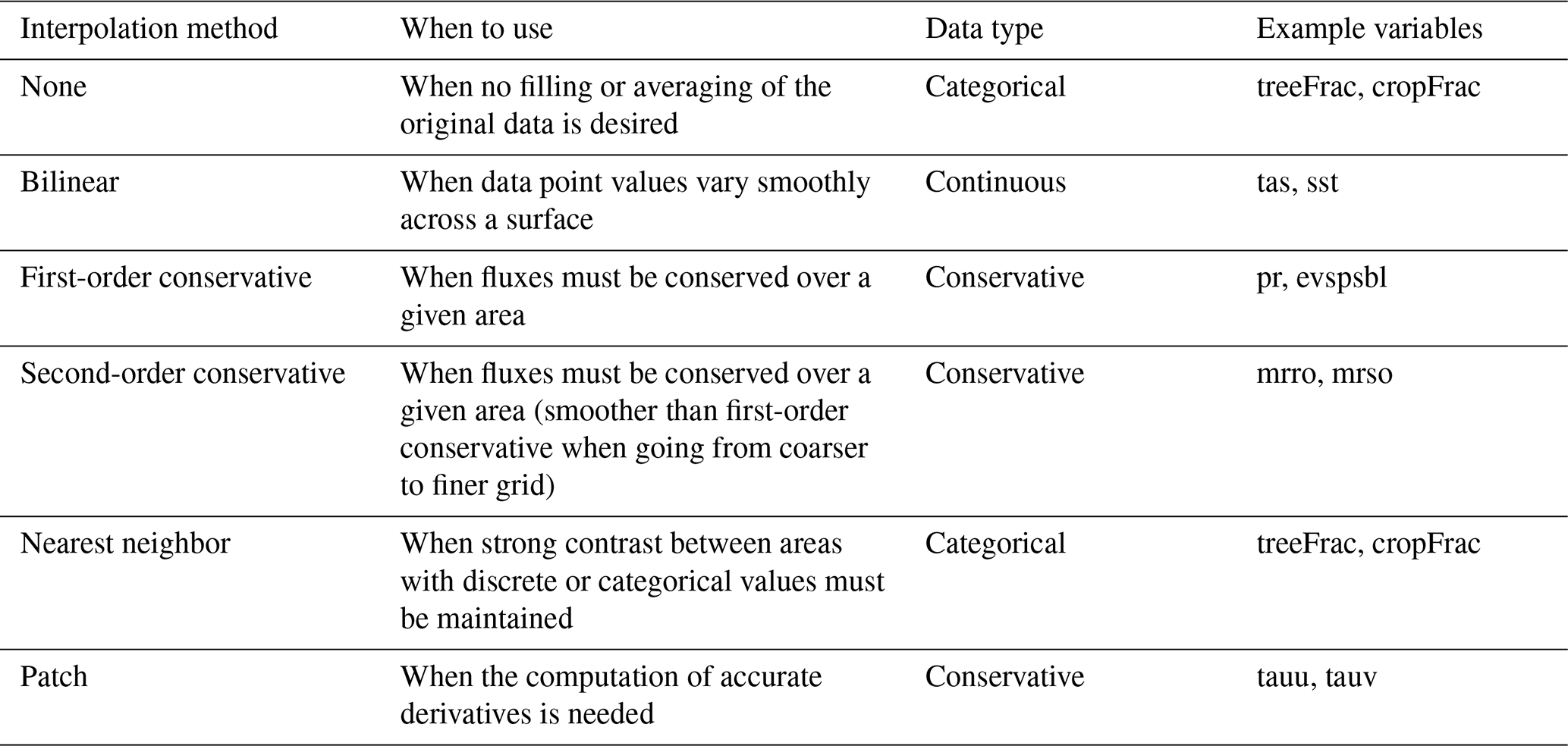
In addition to the variety of spatial resolutions present within an MME, temporal inconsistencies may also exist among members. These arise because models can use different calendar conventions when storing output in the commonly used netCDF format, which supports nearly ten calendar types (NetCDF Users Guide: NetCDF Utilities, 2025) and subsequent different encoded calendars in the modelling centers. The best choice of calendar for a given study will depend on the study particulars and researcher preference. Regardless of this choice, calendars should be brought into alignment during the regridding process to avoid inconsistencies in subsequent MME analyses.

4 Outlook

4.1 Machine Learning

With the rapid production and accumulation of climate data, automated and increasingly sophisticated analysis techniques have become essential (Glymour et al., 2019). Recent advances in ML have been most pronounced at weather timescales, where large training datasets enable robust data-driven approaches. In contrast, applications to climate timescales are more challenging due to limited sample sizes, stronger non-stationarity, and a frequent occurrence of conditions outside the range of the training data, especially for extreme events. Despite these challenges, ML has emerged as a valuable tool for enhancing ensemble approaches in climate science (see Fig. 4).

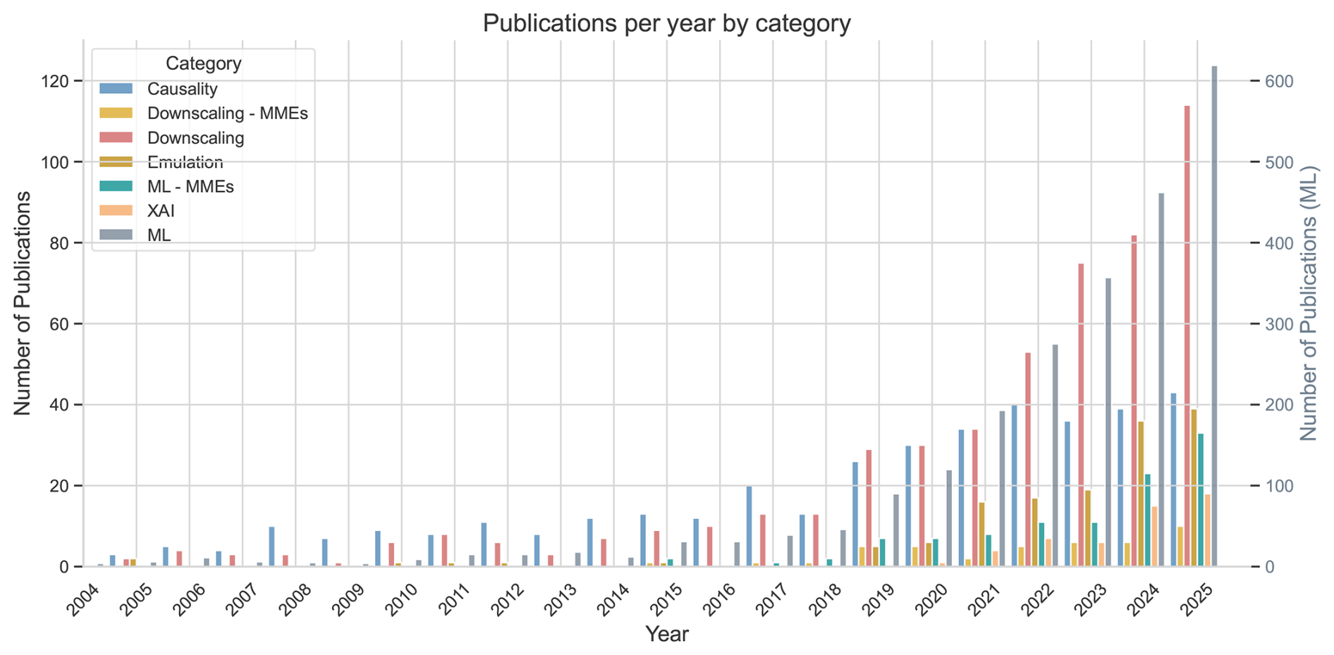
Figure 4 Number of publications per year involving different ML-related techniques in the context of climate modelling: ML (y-axis on the right), ML and MMEs, Downscaling, Downscaling and MMEs, Causality, Emulators, and Explainable AI (XAI). The data was extracted from the citation reports available at Web of Science (https://www.webofscience.com/wos/woscc/basic-search, last access: 14 April 2026) using the queries provided in Supplement S1.

Over the past 5–10 years, ML applications have demonstrated significant advantages in addressing non-linear, high-dimensional, and hierarchical problems (Li et al., 2021 and references therein). By utilizing observational data as either a reference, benchmark, or a constraint, ML offers significant potential to extract additional insights from MMEs. Approaches based on neural networks, causal inference, explainable artificial intelligence (XAI), and nonlinear multivariate emergent constraints have become increasingly competitive with traditional numerical, knowledge-based methods (see Fig. 5 and de Burgh-Day and Leeuwenburg, 2023; Eyring et al., 2024). These capabilities make ML particularly well-suited for identifying patterns and complex physical processes within climate model data, enabling a more comprehensive exploration of the valuable information embedded within the data (Reichstein et al., 2019; Wang et al., 2018). In short, ML has the potential to make climate models better and faster, while reducing their high energy consumption. Nevertheless, the application of ML algorithms in constructing MMEs for climate impact assessments remains at an early stage. Below, we provide an overview of emerging ML approaches for analyzing MMEs.

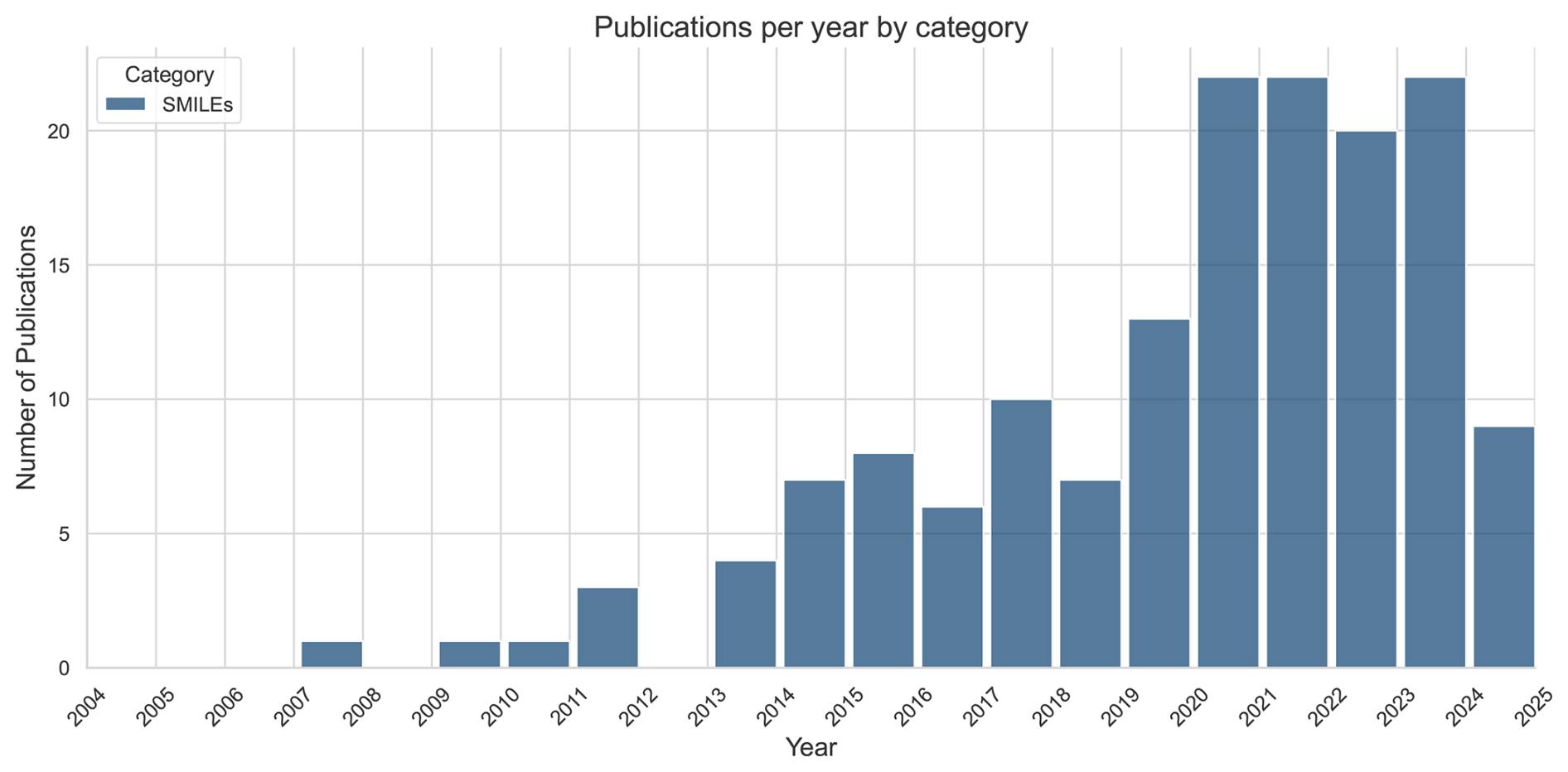
Figure 5 Number of publications per year involving SMILEs. The data was extracted from the citation report available at Web of Science (https://www.webofscience.com/wos/woscc/basic-search, last access: 14 April 2026) for the queries provided in Supplement S1.

4.1.1 Downscaling and Bias Correction

ESMs have horizontal resolutions often far coarser than those needed by decision makers and also exhibit substantial biases (Maraun et al., 2017). Recently, ML has been exploited to bias-correct and downscale MME's outputs – with both processes often done simultaneously. The source data are typically coarse-resolution outputs from climate models for historical periods, while the targets are high-resolution observational datasets, such as gridded products interpolated from gauge stations. It is a common practice to perform dimensionality reduction (e.g. performing principal component analysis on the raw data) before the training process. Multiple ML methods have been tested and compared, including random forests, support vector machines, relevance vector machines, and artificial neural networks (Crawford et al., 2019; Sachindra et al., 2018; Wang et al., 2018; Xu et al., 2020; Dey et al., 2022; Jose et al., 2022; Shetty et al., 2023; Zebarjadian et al., 2024; Li et al., 2021). The domain of these studies is generally limited to river basin scales (Crawford et al., 2019; Dey et al., 2022; Jose et al., 2022; Sachindra et al., 2018; Shetty et al., 2023; Xu et al., 2020; Zebarjadian et al., 2024), although Wang et al. (2018) and Li et al. (2021) obtained good results at a country level for Australia and China. In many of these studies, it has been found that tree-based approaches (like random forests) commonly perform better than other algorithms, making them a strong baseline for future research that aims to improve bias correction or downscaling algorithms.

Although these approaches provide a practical way to leverage MME future projections and observations to obtain a “best estimate” of future quantities, there are several critical limitations to consider. First, within these methods, it is assumed that the relationships between model outputs and observations remain stationary, including model biases and errors (Maraun, 2016). However, skillful or poor model performance during the historical period does not necessarily translate into the same for the future. Training the algorithms with historical data can thus lead to projections becoming overly constrained. Potential solutions for this aspect are to use trend-preserving learning (Wang and Tian, 2024) or climate-invariant ML methods (Beucler et al., 2024).

Another critical aspect that requires further attention in future ML-based bias correction and downscaling efforts is the potential degradation of the representation of temporal variability in final estimates (Shetty et al., 2023). Among the studies mentioned above, only Li et al. (2021) acknowledged that their model outputs showed a significant reduction in the interannual variability relative to the original CMIP models. Thus, it is necessary to implement evaluation metrics for the algorithms that consider aspects such as the standard deviation of the generated time series, the frequency and persistence of extreme events, and the amplitude of different modes of variability. Most approaches aim to minimise only one error metric ignoring the skill regarding other aspects and the physics behind them. For example, the mean precipitation could be improved but the representation of the extreme events or the number of wet days may not be addressed. Algorithms that can minimize multiple loss functions simultaneously could be advantageous to preserve multiple statistical features of the fields of interest (Lin et al., 2019; Sener and Koltun, 2018; Zuluaga et al., 2013). Furthermore, ML-based approaches normally focus on predicting just one variable. Using methods that aim to predict multiple variables could help preserve inter-variable relationships (while also helping preserve different modes of variability).

Finally, most bias correction or downscaling algorithms are trained to predict the outputs in one grid cell based on the nearest CMIP grid cell. This approach neglects spatial relationships contained either within the inputs or the desired outputs. ML methods that account for spatial relationships could be of use, including convolutional neural networks (Gu et al., 2018; LeCun et al., 2015; Wang and Tian, 2022, 2024). Incorporating spatial relationships, multiple variables, and multiple error metrics, also diminishes the impact of observational uncertainty, since physical relationships are more easily preserved, and it also reduces the risk of producing overly constrained projections. Considering the limitations of the approaches mentioned for detecting physically plausible connections, it is essential to explore additional methodologies, with causal inference being one promising option.

4.1.2 Causal inference for climate models

Causal inference aims to identify the causal structure of complex systems such as the Earth and to quantify causal effects by combining domain knowledge, ML models, and data from observations and climate model simulations (Runge et al., 2023, and references therein). Because widely adopted methods based on simple descriptive statistics often fail to accurately capture the underlying physical mechanisms (Beven and Freer, 2001), structural causal models (SCMs) have become a well-established approach in statistics and ML for causal inference (Runge et al., 2019). An important resource in this area is the causality benchmark platform causeme.net, which aims to provide benchmarks with well-established causal structures (Runge et al., 2020). Process-oriented causal analysis has been applied across a broad range of topics, including Arctic processes and their connections to the mid-latitudes (Docquier et al., 2022, 2024; Galytska et al., 2023; Kaufman et al., 2024; Kretschmer et al., 2020; Polkova et al., 2021), Atlantic–Pacific interactions (Karmouche et al., 2023) and subpolar gyre variability (Falkena and von der Heydt, 2025).

Building on this foundation, recent research has increasingly explored the integration of causal discovery with deep learning (DL), presenting a promising avenue for improving climate simulations (Iglesias-Suarez et al., 2024; Kyono et al., 2020; Luo et al., 2020; Wang et al., 2024; Yoon and Schaar, 2017; Zhang et al., 2023). This combination aims to address biases and uncertainties associated with subgrid-scale processes, such as clouds and convection. Previous research has demonstrated DL's capability to effectively represent small-scale processes, such as deep convection, using storm-resolving model simulations (Eyring et al., 2021; Gentine et al., 2018; Grundner et al., 2022). Despite this potential, DL algorithms have been criticised for robustness issues, poor generalization, and the reliance on spurious, non-physical relationships, particularly when conditions diverge from the training data (Brenowitz et al., 2020; Scholkopf et al., 2021; Thuy and Benoit, 2024). However, Iglesias-Suarez et al. (2024) demonstrated that causal discovery can effectively identify the physical drivers of subgrid-scale processes, thereby enhancing the reliability of DL algorithms. Their causally-informed approach generates climate means and variability that closely match original simulations, while preventing spurious links typically seen in traditional DL-based parameterizations. This aligns with previous work by Zhang et al. (2023) emphasizing the value of integrating domain knowledge to address the limitations of purely data-driven models. While these studies currently do not pertain directly to multi-model analysis, their methodologies hold significant potential for future applications in this area.

4.1.3 Process-oriented causal model evaluation

Building on the identification of causal relationships, these frameworks also offer opportunities for systematically evaluating climate models. Detecting similar causal connections in observations and model simulations provides an opportunity to assess model performance that indicates whether models can correctly reproduce processes in the climate system. Such an evaluation framework was first introduced by Nowack et al. (2020) and was termed causal model evaluation (CME). To facilitate the comparison of causal relationships, the authors introduced a modified asymmetric F₁ score metric to classify the agreement between compared causal graphs. A similar approach was proposed by Vázquez-Patiño et al. (2020). Debeire et al. (2025) built their study upon the findings of Nowack et al. (2020) to address the practical challenges of integrating CME for CMIP6 MMEs projections. The authors adopted and adjusted the F₁ score definition and complemented it with a distance metric 1−F₁ with smaller distance values indicating greater similarity, both in terms of performance relative to the reference graph and in terms of dependence among the models. Based on this metrics, Debeire et al. (2025) developed a new weighting scheme, termed causal weighting, inspired by the earlier works of Knutti et al. (2017) and Brunner et al. (2020), which accounts for both model performance and interdependence of causal networks.

Ricard et al. (2024) employed a network-based approach, termed netCS, which leverages sea surface temperature (SST) variability and teleconnections to constrain Equilibrium Climate Sensitivity (ECS) and Transient Climate Response (TCR). The authors argue that the behavior of SST networks serves as a reliable proxy for how models respond to increased CO₂ concentrations. Their results show that some models capture regional SST distributions well but fail to replicate connectivity patterns, and vice versa. This distinction is crucial for evaluating model performance over historical periods, as models that realistically reproduce past SST patterns may exhibit more physically consistent behavior, even if they are not necessarily better tuned. While this does not guarantee that those models are superior for future projections (Rasp et al., 2018; Zhu and Poulsen, 2021), it provides valuable evidence. The authors further propose that causal networks, when used alongside traditional emergent constraints, offer a more reliable framework for ranking climate models in future climate projections.

4.1.4 Machine Learning for Climate System Emulation

Climate model emulators, including surrogate models, are simplified representations of the complex processes embedded in climate models, enabling faster computations and predictions. They mimic the behaviour of a climate model without explicitly solving the underlying equations. ML presents a unique opportunity to emulate components of the climate system through novel and computationally efficient parameterizations. Such approaches have the potential to increase the efficiency of climate simulations while enabling higher resolution simulations (Eyring et al., 2021; Gentine et al., 2018). However, the success of ML emulation of the climate system varies depending on the choice of algorithm, temporal resolution, type of training data, and model complexity (Dueben and Bauer, 2018; Scher, 2018).

One notable initiative in this context is ClimSim, a hybrid physics-ML dataset designed to provide high-quality data for training ML emulators of climate processes (Yu et al., 2023). These datasets have been tested for deterministic and stochastic parameters, and show promise for future climate simulations if applied properly. Future studies could explore the use of MMEs as training data to develop novel ML-based emulators. Complementing the available data to train emulators, Lu and Ricciuto (2019) demonstrate an innovative approach integrating SVD, Bayesian optimization, and neural networks to create a computationally efficient surrogate model. Weber et al. (2020) provide technical notes of ML, using the example of forecasting precipitation under CO₂ forcing. The remarkable computational efficiency and ability of ML emulators to replicate complex climate processes with high precision demonstrates their potential. Nevertheless, several challenges remain, including the high computational cost of running ML models, limited diversity in training data, and the need for more robust methods to evaluate simulations.

4.1.5 Further promising Future ML Avenues

There are numerous promising avenues involving ML for the analysis and processing of CMIP outputs. Explainable AI (XAI), which aims to extract physical insight from otherwise black-box ML models, offers substantial potential for identifying physically meaningful changes in the Earth system simulated by CMIP models (Rader et al., 2022). For example, layer-wise relevance propagation (LRP), has been used to identify the spatial regions and input features that neural networks rely on when generating predictions (Toms et al., 2020) and has proven especially valuable for improving interpretability by visualizing relevance heatmaps (Hilburn et al., 2020; Labe et al., 2024; Labe and Barnes, 2022; Sonnewald and Lguensat, 2021). This interpretability adds value to ensemble evaluation, providing critical information that can inform model weighting schemes. ML also offers effective tools for evaluating both the performance and independence of climate models within MMEs, further supporting the development of ensemble weighting metrics (Brunner and Sippel, 2023). These types of methods also support the development of process-oriented bias correction and downscaling methods for MMEs (Maraun et al., 2017). Furthermore, efforts to predict end-user-relevant variables that are not directly simulated by GCMs, including crop yield (Crane-Droesch, 2018; Sidhu et al., 2023; Veenadhari et al., 2014) and power generation potential (Jung et al., 2021; Nwokolo et al., 2023; Yeganeh-Bakhtiary et al., 2022), demonstrate the potential of ML to enhance the applicability of MMEs for stakeholders and decision-makers. Given ML's growing role in improving climate projections, interpretability, and practical usability, AI-ready databases such as ClimateSet (Kaltenborn et al., 2023) represent valuable resources for the research community.

4.2 Single Model Initial Condition Large Ensembles (SMILEs)

For some activities and experiments, many models in CMIP5 and CMIP6 provide only one ensemble member (Milinski et al., 2020; Olonscheck and Notz, 2017). Consequently, modelling groups strive to provide their best performing members, carefully calibrated to the same internationally available observational datasets. This implicit incentive for modelling groups to add simulations to the CMIP MME that are less extreme can lead to a MME that underestimates the uncertainties. The outcome of this incentive is shown by findings from Sanderson et al. (2008) who found that the standard model performed comparatively to the best-performing model. To address this and other limitations of MMEs based on single-members from different modelling centers, an emerging approach (see Fig. 5) is to include multiple simulations from individual models that differ only in their initial conditions (Maher et al., 2021). When there are at least 10 ensemble members, we refer to the ensembles as SMILE (Deser et al., 2020).

Although MMEs are useful for examining the combined influence of three types of uncertainties in climate projections (model uncertainty, internal variability uncertainty, and scenario uncertainty), MMEs do not allow us to distinguish internal variability from the forced response. On the other hand, SMILEs allow us to quantify internal variability for any given future scenario, independent from model uncertainty (Deser et al., 2012b; Lehner et al., 2020). This capability is particularly powerful for regional detection and attribution studies and for the analysis of extreme climate events (Lehner et al., 2017; McKenna and Maycock, 2021; von Trentini et al., 2020; van der Wiel et al., 2021; Pérez-Carrasquilla et al., 2025).

While large ensemble simulations are well established as essential for studying extreme events (see also Sect. 3.2), they are equally relevant for the analysis of compound events that result from combinations of multiple weather and climate drivers (e.g. simultaneous drought and heatwave; Bevacqua et al., 2022, 2023; Wu et al., 2023). Such events are characterized by complex interactions between extreme conditions across variables, space, or time. Consequently, single variable based approaches may underestimate risks, and neglect the impact of the interplay between different variables. In this context, Bevacqua et al. (2023) showed that attributing compound events requires larger sample sizes than events based on extremes in a single variable, especially when the drivers are weakly correlated and have similar trends. Sampling a wide range of possible atmospheric conditions using SMILEs helps avoid underestimating the frequency and severity of compound events and provides deeper insights into their physical drivers and potential future changes.

When multiple realizations are available, it is considered good practice to average all realizations from each model and incorporate these means into the MME. This approach is appropriate for applications focusing on long-term mean changes or the forced response, but is not appropriate for analyses of extremes or internal variability, where individual realizations carry relevant information. When more ensemble members are used, it is important to remember that the ensemble size available for the individual models should not influence the weight given to this model in the MME (Knutti et al., 2010a). Future studies should provide a methodological framework on how to combine SMILEs and MMEs in the most productive and meaningful way.

Some modelling centers have also applied SMILEs framework to partition the forced response into contributions from individual forcings (e.g. greenhouse gases, aerosols, biomass burning) with single-forcing large ensembles (SFLE; e.g. derived from CESM2 framework; Simpson et al., 2023). These ensembles change only one forcing at a time while holding all others fixed, thereby enabling attribution of the drivers underlying responses identified in all-forcing SMILEs.

One challenge to employing SMILEs is data accessibility. To address this, the Multi-Model Large Ensemble Archive (MMLEA) was developed (Deser et al., 2020). The newly published MMLEAv2 expands upon the original archive by including a larger number of models (18 compared to 7 previously) and more three-dimensional variables (Maher et al., 2025). Both the MMLEAv2 and a suite of corresponding observational datasets have been regridded onto a 2.5° common horizontal grid, reducing data volume and enabling straightforward model-to-model or model-to-observation comparisons. In addition, the release of MMLEAv2 is accompanied by the newest version of the CVDP (CVDPv6; Phillips et al., 2020), introduced in Sect. 2.5.

For a variable with relatively low internal variability or high signal-to-noise ratio, 10 ensemble members can be used to sufficiently detect changes, e.g. for the global mean land temperature (Deser et al., 2012b). To robustly detect significant warming in the 2050s relative to the 2010s (at the 95 % confidence level), Deser et al. (2012b) found that only a single ensemble member was required for nearly all locations. In contrast, precipitation exhibits substantially higher internal variability: detecting changes requires approximately 3–6 ensemble members in the tropics and high latitudes, while more than 15 ensemble members are needed in the mid-latitudes, with estimates reaching up to 40 members (Deser et al., 2012a, b). For sea level pressure, Deser et al. (2012b) reported that only 3–6 ensemble members are sufficient in the tropics, whereas 9–30 are required in the extratropics. The number of ensemble members required varies regionally, reflecting differences in both the strength of the forced signal and local internal variability (Bittner et al., 2016). Over the ocean, less SMILE members are required (Milinski et al., 2020). Table 2 provides a small sample of papers that have employed large ensembles for a variety of research questions.

Table 2 Examples of large ensembles used and how many models were investigated.

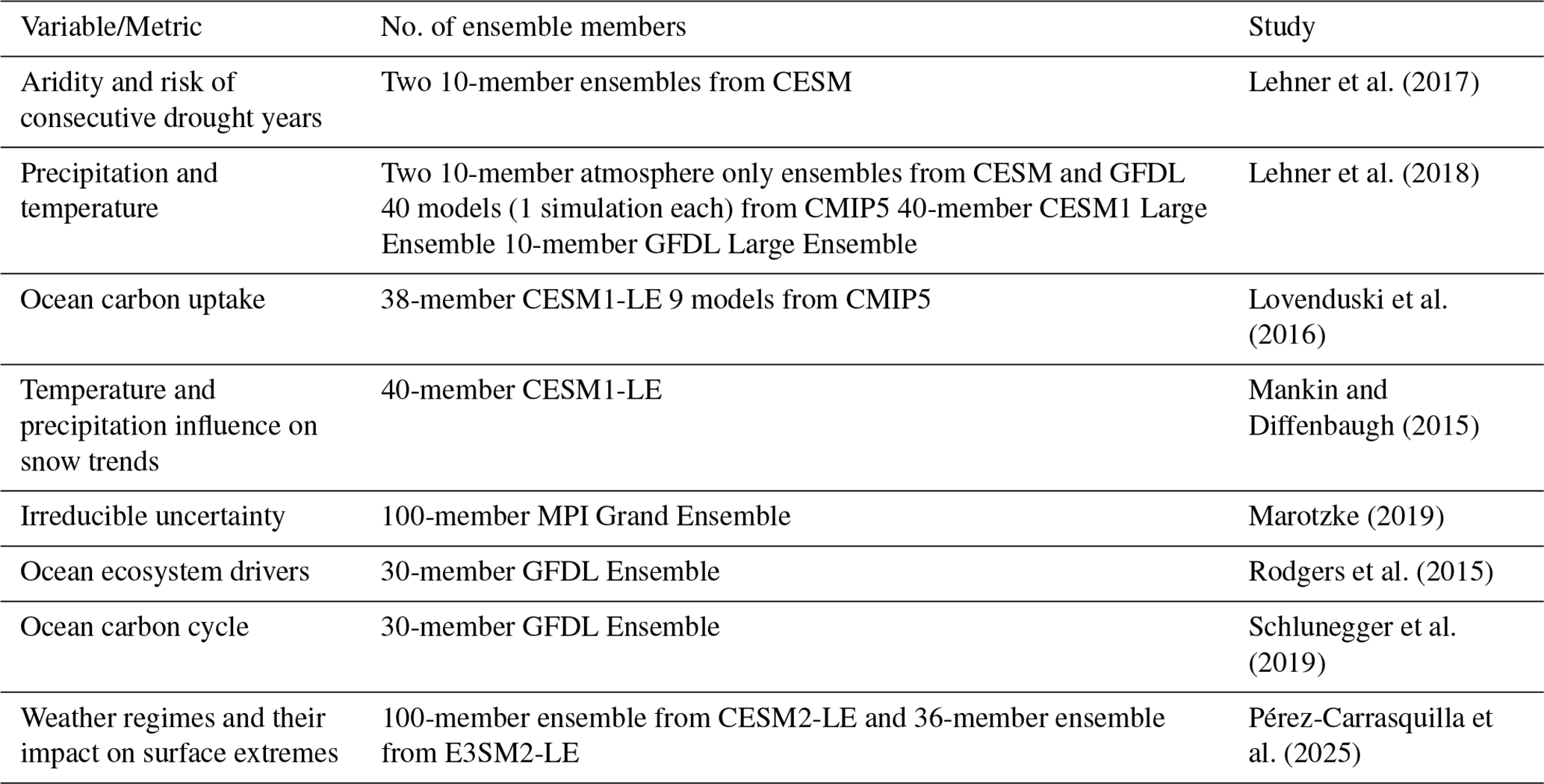
4.3 Computational Resources and Carbon Impact

MMEs, such as CMIP6, are powerful tools for exploring past, current, and future climate conditions, but they come with substantial computational and energy demands. MMEs typically rely on multiple simulations across different models or multiple ensemble members of a single model, performed on high-performance computing (HPC) platforms. These execute calculations across many parallel cores and process and generate large amounts of data that require careful management and optimization. Simulating a century-scale global climate model with high spatial and temporal resolutions can take weeks, even on HPC systems. For example, the MPI-ESM1.2 model in its standard low-resolution configuration (approximately 200 km grid spacing), achieves between roughly 45 and 85 simulated years per day, representing a significant improvement over the 17 years per day achieved during CMIP5 simulations (Mauritsen et al., 2019). On the other hand, running an ultrahigh-resolution climate model in a near-global setup, with ∼ 1 km horizontal resolution reaches a performance of only about 0.043 simulated years per day (∼ 15.7 simulated days per day) (Fuhrer et al., 2018). Computational performance therefore represents a major constraint in the design of ESM experiments, requiring trade-offs between resolution, complexity, and the size of ensembles.

4.3.1 CPMIP metrics for Climate Modelling

Balaji et al. (2017) introduced a universal set of metrics to evaluate HPC and ESM performance, emphasising that traditional metrics (e.g., floating point operations per second) are no longer sufficient to characterize newer generations of computing architectures and the diverse structures of modern ESMs. Given the increasing complexity of ESM components and their heterogeneous computational characteristics, they advocated adopting these metrics (Table 3) as a standard within globally coordinated modelling initiatives and proposed their collection through the Computational Performance MIP (CPMIP). These metrics provide a consistent basis for assessing technological advances in climate models, are accessible from routine production runs, and capture efficiency across the entire modelling lifecycle.

Table 3 List of metrics introduced in CPMIP, adapted from Acosta et al. (2024).

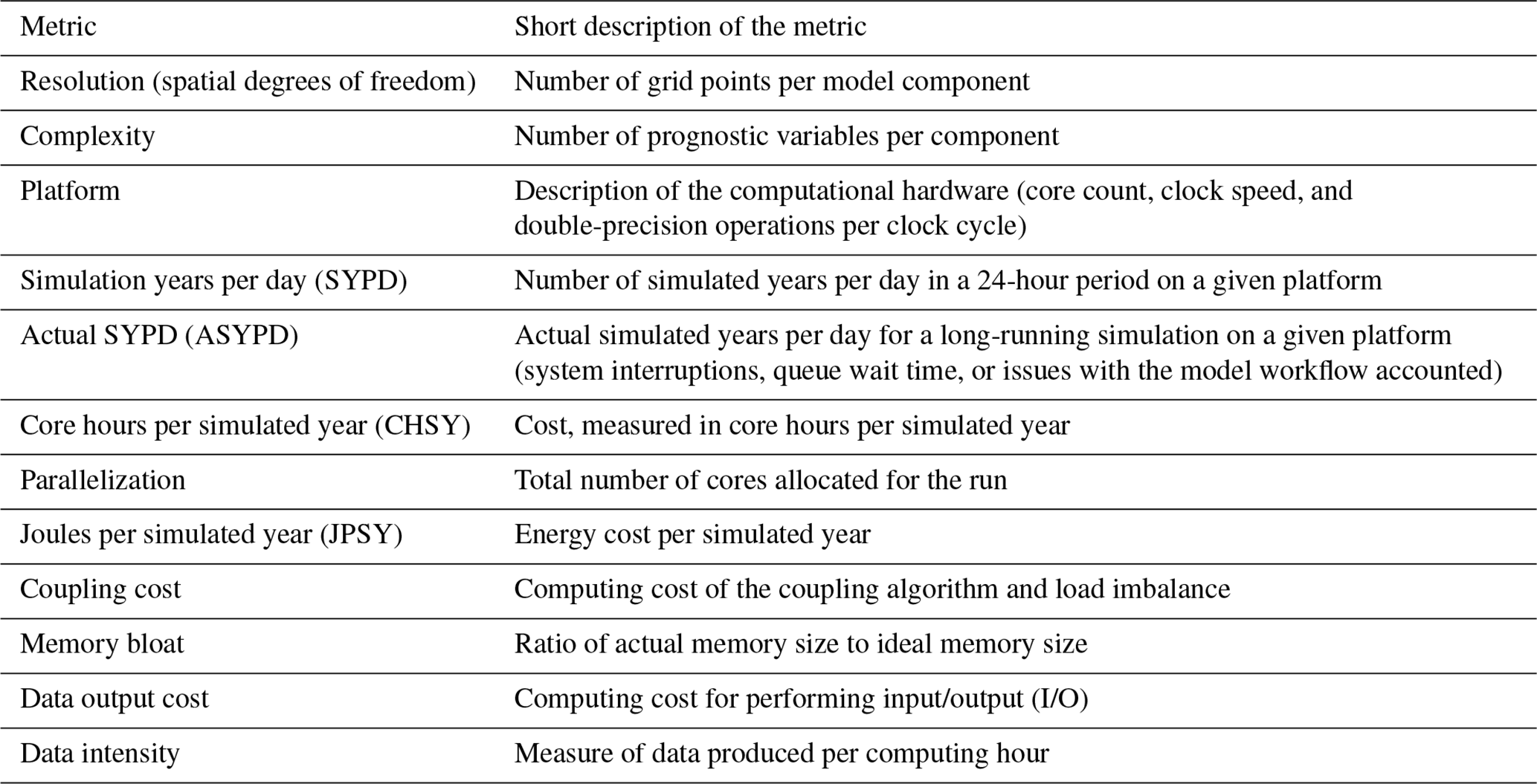
Addressing the performance characteristics of individual models within a MME can contribute to a more balanced and efficient use of computational resources. Building on the foundational CPMIP framework, Acosta et al. (2024) extended this work by incorporating empirical data from CMIP6, collected during long, real-time model runs across 14 institutions, encompassing 33 experiments and nearly 500 000 years of simulations. The study places particular emphasis on energy consumption, data storage demands, and operational efficiency, and provides strategic recommendations for improving the sustainability and performance of future climate modelling efforts.

The demand for computing power is steadily increasing due to several factors, including higher spatial and temporal resolution, the explicit representation of complex climate processes that were previously parameterized, increasing ensemble sizes, and the associated growth in data storage requirements for both input and output. Improving model accuracy through these processes leads to more detailed spatial and temporal outputs, but requires immense computational resources. For example, Flato (2011) found that increasing model resolution from 200 to 20 km demands roughly 10 000 times more computing power.

Kilometer-scale simulations of individual models and associated MMEs are being actively developed (Ban et al., 2021; Coppola et al., 2020; Pichelli et al., 2021; Rackow et al., 2025), as well as coordinated intercomparisons for global storm-resolving models (GSRM). To cope with the high computational and energy demands required for increase in resolution and process detail (Schär et al., 2020), such simulations are often conducted over limited regional domains (Coppola et al., 2020; Nolan and Flanagan, 2020), rely on simplified parameterizations (for processes such as radiation or soil interactions) or – when performed globally – are restricted to relatively short simulation periods of only a few weeks (Schär et al., 2020). However, this limitation is rapidly being overcome, with multi-year global simulations at such resolutions have already been conducted using models such as ICON in its Sapphire configuration (Hohenegger et al., 2023), the eXperimental System for High-resolution prediction on Earth-to-Local Domains (X-SHiELD) (Guendelman et al., 2024; Merlis et al., 2024), or the IFS model coupled to the Finite-volumE Sea ice-Ocean Model (Rackow et al., 2025).

Beyond the role of resolution and resolved processes, the internal structure of ESMs also plays a crucial role in determining computational performance. ESMs are structured with a component-based architecture, allowing scientists to update or add new components over time. While this architecture enables continuous flexibility, it also brings software engineering challenges. Modifications to individual components can alter computational demands and affect data processing, input/output (I/O) operations, and network traffic (Wang and Yuan, 2020). As shown in Acosta et al. (2024) coupling components, which synchronize different processes, adds up to 5 %–15 % overhead to execution costs.

Operational factors such as job scheduling also influence computational efficiency. Queue times significantly impact overall execution speed and efficiency, although they vary across different institutions (Acosta et al., 2024). Short and consistent queue times are beneficial for MMEs, as they help ensure the timely completion of simulations. Reducing queue times improves the effective use of available HPC resources, allowing more simulations to be completed within a given timeframe and thereby increasing the overall throughput of the ensemble.

4.3.2 Carbon Footprint of Climate Modeling: Towards ”greener” Hardware

Running climate models on HPCs, particularly for large-scale MMEs, requires substantial energy and is associated with a significant carbon footprint. The climate modelling community is aware of this and is exploring ways to optimize code efficiency and transition to greener energy sources to minimise the carbon impact of their research efforts. In this context, CPMIP focuses on capturing the real energy costs of running models, aiming to help climate scientists make eco-friendly decisions in computing. Using the CPMIP metrics and the efforts of the Infrastructure for the European Network for Earth System Modelling Phase 3 (IS-ENES3) project (Joussaume and Budich, 2013), the total computational energy costs of climate experiments have been assessed, enabling estimates of the associated carbon footprint (Acosta et al., 2024). For 8 out of 49 institutions that were involved in CMIP6, the total estimated emissions amount to 1692 t CO₂ (with total energy costs ranging from 0.41 TJ to 26.70 TJ). For context, the International Energy Agency (IEA) reports that the “global average energy-related carbon footprint” is approximately 4.7 t CO₂per person and per year. Thus, the total emissions from this share of CMIP6 modelling centers are roughly equivalent to the annual energy-related emissions of 360 people.

As researchers recognize the environmental impact of extensive model runs, eco-friendly hardware is becoming an increasingly important consideration in HPC for climate modelling. One example of this good practice is the Energy-efficient climate simulations on heterogeneous supercomputers through co-design (EECliPs) project led by German Climate Computing Centre (Deutsches Klimarechenzentrum, DKRZ; https://www.dkrz.de/en/projects-and-partners/projects-1/eeclips, last access: 14 April 2026), aiming to improve simulation quality while reducing the energy requirements of the ESM ICON (Adamidis et al., 2025). By encouraging institutions to collect the data needed to estimate their carbon footprint, to adopt eco-friendly hardware and to implement thoughtful modelling practices, the climate modelling community can reduce its carbon impact while continuing to advance its scientific mission.

4.3.3 HPC Facilities: petascale and beyond

As climate models continue to evolve, HPC facilities operating at the petascale and beyond are necessary. Looking ahead, exascale computing systems, capable of achieving 10¹⁸ floating-point operations per second, promise to greatly expand modelling capabilities, enabling longer, higher-resolution simulations, more complex process representation, and improved exploration of predictability limits in ESMs. This potential led to the launch of many projects aiming to develop and optimize the parallel execution on exascale systems (Adamidis et al., 2025; Taylor et al., 2023; https://www.fz-juelich.de/en/ias/jsc/projects/ifces2, last access: 14 April 2026).

In the context of the increasing computational complexity, the findings from the CPMIP and performance metrics applied to CMIP6 experiments underline the need for better optimization of model configurations, improved coupling mechanisms, and more efficient use of HPC resources. The intercomparison between models and institutions reveals significant differences in computational costs, highlighting the need and potential for strategic advancements. Coordinated efforts are also required to integrate the latest technological advances, as e.g. outlined in Sect. 4.1 and 4.2. Standardized measurements of computational and energy costs can guide the path forward, ensuring that model performance is comparable, and thereby allowing researchers to identify areas for improvement and make informed decisions in the development.

5 Concluding Remarks

Climate modelling has been key to the understanding of past, present, and future climate change. It is a dynamic field, profiting from growing computational capacities and advances as well as benefits from the increasing understanding of physical and chemical phenomena. Climate projections rely on MMEs to assess uncertainties and improve their robustness. This review synthesizes key practices, challenges, and emerging approaches in working with MMEs, drawing on the collective insights of the Fresh Eyes on CMIP community. By examining model evaluation strategies, model dependence, selection and weighting methods, and uncertainty quantification, we aim to support researchers in making informed choices when designing MME studies – while fully acknowledging that the diversity of research questions makes it impossible to create a set of universally transferable recommendations. We further highlight the growing relevance of ML and SMILEs, which are shaping the future of climate ensemble analysis, particularly in the context of CMIP7. Finally, we advocate for awareness of the computational costs associated with climate modelling and analyses.