Emerging global freshwater challenges unveiled through observation-constrained projections

Future hydrological projections exhibit significant discrepancies among models, undermining confidence in the predicted magnitude and timing of hydrological extremes. Here we show that observation-constrained changes in global mean terrestrial water storage (TWS), excluding Greenland and Antarctica, could be approximately 83 mm lower than raw projections from the Inter-Sectoral Impact Model Intercomparison Project phase 3b (ISIMIP3b) by the end of this century under both the low (SSP1-2.6) and high (SSP3-7.0) future forcing scenarios. Notably, the 95th percentile upper bounds are substantially reduced from 2 to −96 mm under the low-emissions scenario and from 8 to −105 mm under the high-emissions scenario, revealing a notable overestimation of global freshwater availability in the raw model projections. Global models are intricate process representations, making it challenging to isolate causes of their differences with observations. However, by leveraging the emergent constraint (EC) methodology and inter-model spread to empirically adjust biases against observations, we derive more tightly constrained estimates of future TWS changes than those obtained from conventional, unconstrained approaches. The EC-corrected estimates are substantially lower than the raw ISIMIP3b projections, implying that current water resource planning may underestimate the severity of future water shortages, particularly if global water demand remains stable or continues to rise. Our findings pinpoint the urgent need to reduce model uncertainties and enhance the reliability of future hydrological projections to better inform water resource management and climate adaptation strategies.

1 Introduction

Terrestrial water storage (TWS) encompasses all water stored on and beneath the land surface, representing the net balance of precipitation, evapotranspiration, and runoff (Getirana et al., 2017; Rodell and Famiglietti, 2001). As a critical element of the hydrological cycle, TWS plays a key role in regulating freshwater availability (Rodell and Famiglietti, 2001) and Earth's energy budget (Getirana et al., 2017), supporting freshwater ecosystems (Tapley et al., 2019; Wu et al., 2024), influencing biogeochemical cycles (Rodell et al., 2018), driving socioeconomic development (Scanlon et al., 2023; Vörösmarty et al., 2000), and mitigating sea level rise by enhancing continental water storage (Tapley et al., 2019).

A warming climate impacts TWS by accelerating the hydrological cycle through enhanced evapotranspiration and by modifying global precipitation patterns (Dai et al., 2018). These changes can exacerbate freshwater scarcity in many regions while increasing flood risk in others, highlighting the crucial need for accurate future projections. However, the discrepancies among models in simulating historical hydrological budgets lead to substantial differences in their projections of extreme hydrological events (Herrera-Estrada et al., 2017; Trenberth et al., 2003; Vogel et al., 2018), which in turn reduce confidence in the predicted magnitude and timing of these extremes. These discrepancies can be attributed to various factors, including uncertainties in climate forcing (Scanlon et al., 2018), the absence of key components such as surface water storage, groundwater storage, and human interventions in most land surface models (LSMs), as well as limited storage capacities within both LSMs and global hydrological models (GHMs).

Modeling uncertainties pose a major challenge to producing reliable projections of future freshwater availability. To address these uncertainties, the emergent constraint (EC) approach has been widely applied to identify statistical relationships across global climate models between observable historical climate metrics and projected future responses (Brient, 2020; Hall et al., 2019). These relationships are not evident in individual models but emerge only when large ensembles are analyzed. Specifically, the EC technique aims to reduce the often uncomfortably large spread in future projections within multi-model ensembles, thereby providing more tightly constrained estimates of variables of interest (Hall et al., 2019). Such improved and physically informed constraints are crucial for climate mitigation and adaptation policymaking. While a large number of ECs have been proposed for global mean temperature changes and other hydro-climatic variables (Bowman et al., 2018; Brient, 2020; Hall et al., 2019; Petrova et al., 2024; Shiogama et al., 2022), the potential constraints on global mean changes in terrestrial water storage remain largely unexplored, probably due to the complex and heterogeneous components of land water storage, their differing representations across numerical models, and the historical lack of continental-scale TWS observations. The launch of the Gravity Recovery and Climate Experiment (GRACE) and GRACE-Follow On (GRACE-FO) missions has, however, provided spaceborne measurements of global freshwater changes (Tapley et al., 2019; Velicogna et al., 2020). Here, we combine a proposed EC with historical GRACE observations and the latest datasets from the Inter-Sectoral Impact Model Intercomparison Project phase 3b (ISIMIP3b; https://protocol.isimip.org/#/ISIMIP3a, last access: 8 July 2024). By incorporating as many models and ensemble members as possible to account for varying model representations, we apply the EC framework to constrain projections of future TWS changes.

2 Data and methods

2.1 Observations

Global TWS anomaly products (excluding Greenland and Antarctica) for the period 2004–2023 were derived from GRACE and GRACE-FO satellites. The period 2004–2023 is shorter than the conventionally defined climatological baseline, but it provides a reasonable basis for estimating long-term trends. In addition, given that our primary focus is on long-term changes in TWS rather than interannual variability, this study period is considered adequate, though longer records would further strengthen the analysis. Because research has demonstrated that GRACE data processing in terms of mass concentration (mascon) solutions results in higher correlations with in situ data compared to spherical harmonic solutions (Watkins et al., 2015), we utilized all three available GRACE mascon solution datasets (i.e., JPL RL06.3M v04, CSR RL0603M, and GSFC mascon RL06 v1.0), produced by the Jet Propulsion Laboratory (Watkins et al., 2015), the Center for Space Research (Save et al., 2016), and the Goddard Space Flight Center (Luthcke et al., 2013), respectively, to estimate observational uncertainty. Missing months in the GRACE time series were filled using linear interpolation. This approach is appropriate because the analysis focuses on long-term changes and linear trends in TWS, rather than on resolving seasonal variability. Furthermore, no scaling factors were applied, as previous studies have indicated that standard scale factors may not improve the accuracy of TWS trend estimates (Humphrey et al., 2023). The mean of three mascon products was used for EC calibration, with the associated standard deviation representing observational uncertainty.

2.2 Global models and climate forcing

Five LSMs and GHMs (see details in Table S1 in the Supplement) from the ISIMIP3b were employed to assess historical and future relationships in TWS anomalies (see details below). These projections were based on climate forcing from the Coupled Model Intercomparison Project Phase 6 (CMIP6) (Eyring et al., 2016). Climate forcing data were sourced from five general circulation models (GCMs) – GFDL-ESM4, IPSL-CM6A-LR, MPI-ESM1-2-HR, MRI-ESM2-0, and UKESM1-0-LL – under three scenarios: historical climate (HIST, 1850–2014), a low greenhouse gas (GHG) emissions scenario (shared socioeconomic pathway (SSP)1-2.6), and a high GHG emissions scenario (SSP3-7.0). These scenarios were selected to maximize the number of available models and ensemble members included in the analysis, thereby enhancing both model diversity and within-model ensemble completeness. The historical climatology (2004–2023) was constructed by combining the end of the HIST run with the beginning of the SSP1-2.6 simulation, following the approach adopted in previous TWS studies using the ISIMIP datasets (e.g., Pokhrel et al., 2021). SSP2-4.5, a “middle of the road” scenario, would be the most appropriate for extending the historical period due to its alignment with historical socioeconomic trajectories (Fricko et al., 2017). Nevertheless, only a limited number of models provide the SSP2 forcing in the ISIMIP datasets. Consequently, trade-offs were required to maintain sufficient model diversity. While the use of SSP1-2.6 to extend the historical climatology may introduce discontinuities in forcing conditions, this approach enables a more comprehensive ensemble analysis. Each individual model realization was treated independently during the EC processing. To further ensure robustness, the proposed ECs were repeated using an ensemble of simulations from eight ISIMIP2b models (Table S2). These simulations were based on climate forcing from four CMIP5 GCMs under three scenarios: historical climate (HIST, 1861–2005), the Representative Concentration Pathway (RCP)2.6 scenario, and the RCP6.0 scenario. All outputs were provided at a monthly temporal resolution and on a 0.5°×0.5° global grid. Monthly data were then regridded to a common 1°×1° global grid using bilinear interpolation. The ensemble members (i.e., outputs from each GHM or LSM driven by different climate forcings) were compared with GRACE data. To ensure consistency, we computed TWS anomalies at each grid point relative to a baseline period of 2004–2009. This aligns all datasets to a common reference, conducting direct comparison of observed and simulated TWS anomalies as deviations from the same climatological mean. Consequently, historical and future climatologies can be derived from these TWS anomalies (see details in the next subsection). While the baseline period is relatively short (affecting only the calculation of anomalies), our analysis focuses on long-term TWS changes, which are expected to be minimally influenced by the length of the chosen baseline.

2.3 Emergent constraint approach and calibration

To implement the EC framework, we begin by identifying statistically significant relationships between projected future annual global mean changes in TWS (e.g., at mid-century or by the end of the century), the predictand y, and historical climatologies (2004–2023) of annual global mean TWS anomalies, the predictor x, across a suite of global models. To ensure the robustness of our EC results, we additionally used linear trends of historical TWS anomalies as alternative predictors. The long-term trend in historical annual TWS anomalies at each grid point was estimated using ordinary least squares regression. A two-sided linear least-squares regression model was then employed to depict the EC relationship between x and y at the global scale. A total of 25 and 31 individual realizations were included in the EC relationships using ISIMIP3b and ISIMIP2b datasets, respectively (Fig. S1 in the Supplement). The nonparametric Spearman rank-order correlation coefficient was also calculated, with corresponding p-values used to assess statistical significance. Residual plots were employed to identify outliers that consistently deviate from the regression-defined EC relationship across scenarios and to evaluate the linearity assumption of the regression.

Once x was estimated from historical GRACE observations, the resulting regression was applied to narrow the inter-model spread of y. In particular, by substituting x with the mean of historical observations, we derived the mean of EC-corrected changes from the regression model. No bias correction was applied before the regression. We further calibrated the projected future changes by applying the EC relationship to each grid cell, resulting in the spatial distribution of EC-corrected projections along with the corresponding biases. It should be noted that if observational uncertainties and regression residuals are large, these errors may propagate through the EC calibration, resulting in less well-constrained projections.

To estimate the uncertainty of the calibrated future changes, a stationary bootstrap method (Brient, 2020; Politis and White, 2004) was applied. Bootstrapping was performed 500 times, generating 500 regression line samples. This approach robustly quantifies the sampling uncertainty without requiring assumptions about the underlying probability distributions. Following the method of Brient and Schneider (Brient and Schneider, 2016), confidence intervals for the calibrated future changes were estimated by projecting the observed value x_o from each GRACE dataset (using all three mascon solutions) onto the generated 500 regression line samples.

Spearman's rank correlation coefficients were calculated for TWS-related variables, including precipitation, evapotranspiration, and total runoff, to elucidate the potential physical mechanisms underlying the EC relationship. Partial Spearman's correlation analysis was also employed between TWS and the other variables, controlling for precipitation effects. These variables were derived from simulations under the historical and SSP3-7.0 scenarios. To understand the spatial distribution of differences in future changes, we categorized the six driest and six wettest ensemble members (Table S1) using the 25th and 75th percentiles of the ensemble distribution of the historical climatology of annual global mean TWS anomalies, after excluding outliers identified from the residual analysis (Fig. S9). For simplicity, we refer to models with historically low and high simulated TWS anomalies as “dry” and “wet” models, respectively.

3 Results

3.1 Proposed emergent constraint derived from historical climatology

Our approach follows established EC protocols by relating an observable historical metric (that is, area-weighted global mean of annual climatologies of TWS anomalies) to a targeted future change (global mean of end-of-century annual TWS change) across an ensemble of models. This strategy is consistent with prevailing EC studies (e.g., Cai et al., 2025; Dai et al., 2024; Kim et al., 2023; Petrova et al., 2024), which often relate present-day climatological states (or trends when they offer stronger physical connections) to future changes rather than link historical and future trends directly. To align GRACE observations with model outputs, we first compute TWS anomalies at each grid point relative to a baseline period of 2004–2009. Anchoring all datasets to this common reference ensures that both historical and future TWS anomalies (whether from observations or models) are directly comparable as deviations from the same climatological mean. Consequently, because both historical and future TWS anomalies share this baseline, their difference naturally represents changes in TWS (hereafter referred to as “TWS change”) rather than changes in anomalies. In fact, our approach to calculating TWS change has shown results comparable to the conventional method (cf. Fig. 2c, d in this article with Fig. 1b, d in Pokhrel et al., 2021). Finally, we derive climatologies of TWS anomalies by averaging monthly anomalies for each calendar year and then computing the multi-year mean over the period of interest.

We analyze historical and future relationships in TWS using multi-model hydrological simulations, including 25 ensemble members from the ISIMIP3b (Warszawski et al., 2014) and 31 ensemble members from the ISIMIP2b (Frieler et al., 2017), considered separately (Methods and Tables S1 and S2). Future projections are based on climate forcing from the CMIP6 (Eyring et al., 2016) and CMIP5 (Taylor et al., 2012), respectively. To maximize the inclusion of available models and compare with previous studies (e.g., Pokhrel et al., 2021), we select a low-emissions scenario (SSP1-2.6/RCP2.6) and a high-emissions scenario (SSP3-7.0/RCP6.0). Significant positive correlations (R>0.99 for both ISIMIP2b and ISIMIP3b models) are found between historical and late century annual area-weighted global mean TWS anomalies across realizations, irrespective of the emissions scenario (Fig. S1). Statistical significance is adjusted for the number of realizations (25 for ISIMIP3b and 31 for ISIMIP2b). These findings indicate that models simulating higher TWS anomalies in the historical climate tend to predict higher TWS anomalies in the future, in agreement with the “wet-gets-wetter” atmospheric response to warming identified globally (Held and Soden, 2006) and over land (Petrova et al., 2024) in the CMIP models. Various hydrological datasets also corroborate this “wet-gets-wetter” signal over water-sufficient lands (Greve et al., 2014; Kumar et al., 2015; Markonis et al., 2019). GHMs and LSMs are developed based on distinct numerical frameworks and parameterizations, leading to structural diversity in how they represent key storage components. This structural diversity (such as lack of surface water and groundwater storage compartments and human intervention in most LSMs; see Tables S1 and S2) is responsible for inter-model differences (Scanlon et al., 2018), which may lead to the “wet-gets-wetter” pattern. For instance, under the SSP1-2.6 scenario, MIROC-INTEG-LAND simulates relatively low climatologies of TWS anomalies in both historical and future periods, whereas JULES-W2 produces much higher values under the same conditions (Fig. S1). Our methodology does not assume identical storage physics across models; instead, it leverages the multi-model spread to empirically constrain biases against GRACE observations.

Notably, however, the strength and spatial extent of the “wet-gets-wetter” response are sensitive to differences in study periods, datasets, and the variables used to characterize hydrological conditions. For example, even when historical and future periods are held fixed, analyses based on satellite observations, GHM/LSM outputs, and GCM simulations report that the “wet-gets-wetter” response spans ∼ 11 % to ∼ 41 % of global land area, as quantified using a nondimensional TWS drought severity index (Xiong et al., 2022).

As shown in Fig. 1, the magnitude of future TWS increases is positively correlated with the historical climatology of TWS anomalies. The Spearman's rank correlation coefficients between the historical climatology and mid-century TWS changes are 0.79 and 0.70 (p<0.01) for the ISIMIP2b and ISIMIP3b ensembles, respectively, under the low-emissions scenario. Under the high-emissions scenario, statistically significant correlations of 0.61 and 0.71 (p<0.01) are observed for the ISIMIP2b and ISIMIP3b ensembles, respectively. For late century TWS changes, significant correlations with the historical climatology persist across both ISIMIP2b and ISIMIP3b ensembles. Residual plots are used to assess the linearity assumption underlying the EC framework (Fig. S9). Overall, the linear EC assumption is broadly reasonable across the four SSP panels. However, late-century projections show residuals that are not fully captured by a single linear EC regression, indicating increased nonlinearity and warranting caution in the interpretation of late-century results. It is worth noting that several modeling factors including initial conditions, structural differences (especially the diversity of storage compartments), human intervention, and calibration can contribute to the large inter-model spread and thus the resulting discrepancies with GRACE observations.

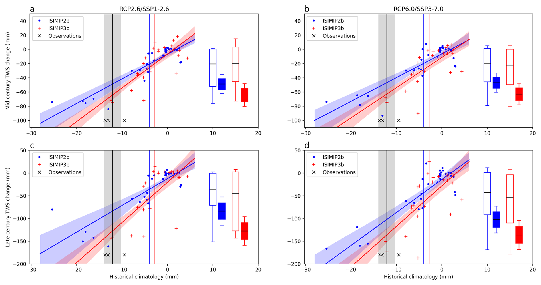
Figure 1 Inter-model relationships between historical (2004–2023) climatologies and future changes at mid-century (2040–2059; upper panels) and late century (2080–2099; lower panels) from ISIMIP2b (blue) and ISIMIP3b (red) models under the RCP2.6/SSP1-2.6 (a, c) and RCP6.0/SSP3-7.0 (b, d) scenarios. Dots and crosses represent global (excluding Greenland and Antarctica) averages from ensemble members. Blue and red lines represent linear regression fits, with 90 % confidence intervals estimated through bootstrapping. Blue and red vertical lines mark the ensemble mean. Black vertical lines indicate the average of GRACE observations (black cross), and grey shading represents the standard deviation. Box plots indicate the mean (black line), 66 % (box), and 90 % (whisker) confidence intervals of future TWS changes before (empty box) and after (filled box) applying observational constraints.

The robust relationship provides a basis for constraining future TWS changes. After applying the EC calibration (Methods), mid-century global mean TWS changes are reduced by 44 and 40 mm compared to the raw projections from the ISIMIP3b ensembles under the low- and high-end forcing scenarios, respectively (Fig. 1, upper panels). For late century projections, EC-corrected changes could be ∼ 83 mm lower than the raw estimates from the ISIMIP3b ensembles irrespective of the forcing scenario (Fig. 1, lower panels), highlighting potentially lower global freshwater availability than initially indicated by the ISIMIP3b models. Furthermore, the EC correction constrains the uncertainty in late century TWS changes by 63 % for the SSP1-2.6 scenario and 69 % for the SSP3-7.0 scenario, based on the 5 %–95 % ranges of future projections, with 90 % confidence intervals estimated via bootstrapping. Specifically, the upper bound (95th percentile) is reduced from 2 to −96 mm under the low-end forcing scenario and from 8 to −105 mm under the high-end forcing scenario, indicating an initial overestimation of global freshwater availability in the raw ISIMIP3b ensemble projections. Global models are sophisticated process representations, making it challenging to isolate causes of their differences with GRACE (Haddeland et al., 2011). However, by leveraging the EC methodology and inter-model spread in water storage partitioning constrained by GRACE observations, we produce more tightly constrained estimates of future TWS changes than those obtained from conventional approaches, while recognizing the inherent uncertainties associated with observational constraints. Note that the reduction in ensemble uncertainty shown in our study is unexpectedly greater than that reported in previous EC-related research (e.g., Brient, 2020; Brient and Schneider, 2016; Petrova et al., 2024), highlighting a potential limitation of the EC approach when applied to freshwater availability. This discrepancy arises because GRACE products used for EC correction are all derived from a single source – the GRACE satellites – resulting in an underestimated uncertainty for TWS observations compared to other multi-source observational variables, such as air temperature and precipitation. EC-corrected changes based on the ISIMIP2b models show results similar to those from the ISIMIP3b models, albeit with higher ensemble averages, which can be attributed to the shallower slopes observed in their linear regression relationships. As ISIMIP2b and ISIMIP3b provide different sets of GHMs/LSMs and ensemble members, driven by different GCMs, these differences may also contribute to discrepancies in the EC-corrected results between ISIMIP2b and ISIMIP3b. Although here we illustrate results using three mascon-based GRACE datasets, extending the analysis to include four spherical-harmonic solutions yields EC-corrected projections that remain robust but produces slightly higher mean TWS changes at the end of this century (Fig. S7). We also analyze the past-future EC relationship using linear trends of historical TWS anomalies as potential predictors (Fig. S2, lower panels). The corresponding results closely align with those obtained using historical climatology of TWS anomalies as predictors, showing identical ensemble averages and consistent 5 %–95 % ranges. Therefore, subsequent analyses are based on the past-future EC relationship with historical climatology of TWS anomalies as predictors, due to the current models' inability to accurately simulate the large regional TWS trends observed by GRACE (Scanlon et al., 2018). This limitation may reduce the reliability of the spatial patterns in future TWS change projections presented below.

3.2 Spatial patterns in future TWS change projections

By the end of the 21st century, TWS is projected to decrease considerably across several regions under the SSP1-2.6 scenario, including the southern United States, Mexico, northwestern South America, both coasts of the strait of Gibraltar, the majority of Central, West, and South Asia, as well as North China (Fig. 2a). Under the SSP3-7.0 scenario, although the spatial pattern of TWS changes is similar, the signal becomes much stronger, especially in the low latitudes (Fig. 2b). The future changes projected by the ISIMIP2b ensembles are consistent with those from the ISIMIP3b ensembles across most land areas, with pattern correlations of 0.44 and 0.55 under the low- and high-end forcing scenarios, respectively. Although this study uses an unweighted ensemble mean and a slightly different period to represent the late century, the spatial distributions closely align with those reported by Pokhrel et al. (2021). The main difference lies in the latitudinal mean, which in our analysis reveals a much steeper decline in TWS over the northern midlatitudes, irrespective of the emissions scenario (Fig. 2c, d).

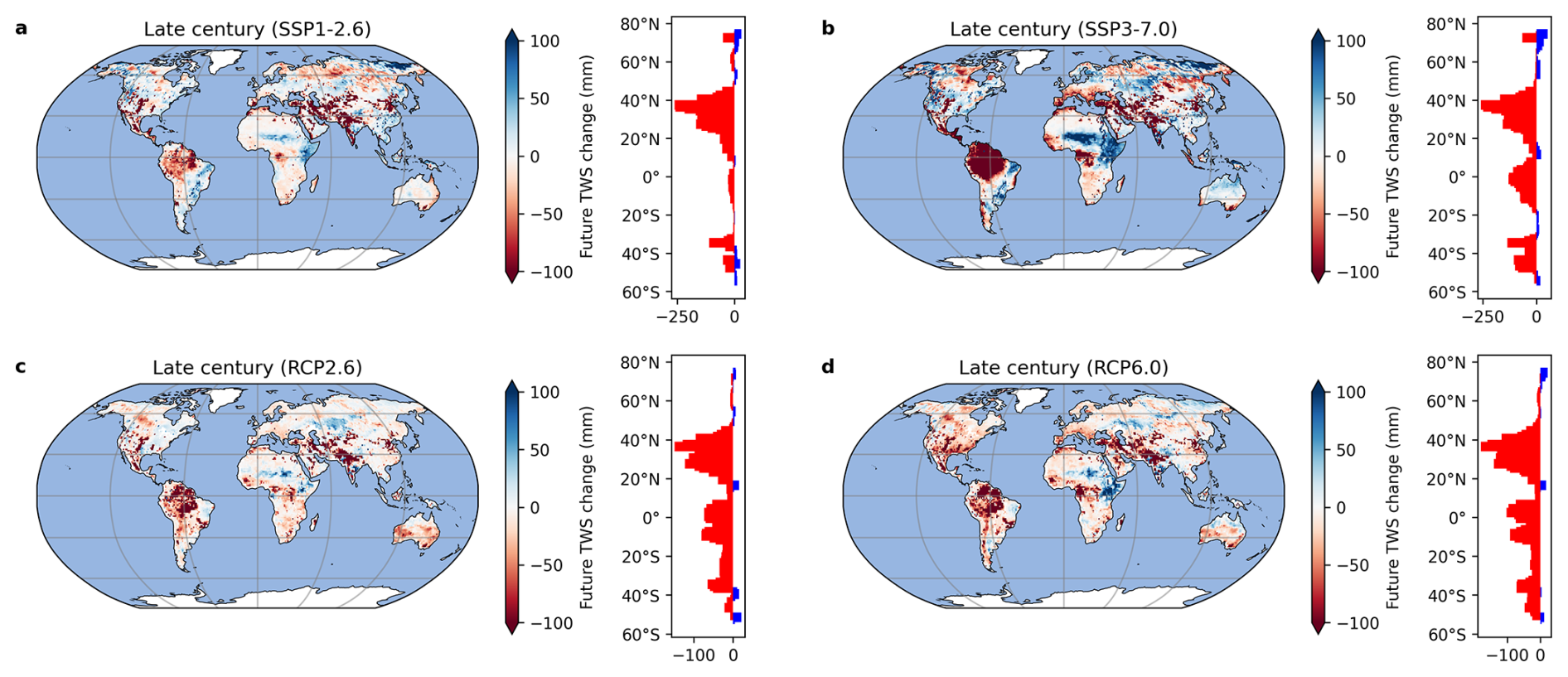
Figure 2 Late century (2080–2099) multi-model ensemble averages of TWS changes under the SSP1-2.6/RCP2.6 (a, c) and SSP3-7.0/RCP6.0 (b, d) scenarios, shown relative to historical (2004–2023) climatologies. The accompanying histograms on the right indicate zonally averaged TWS changes for each scenario.

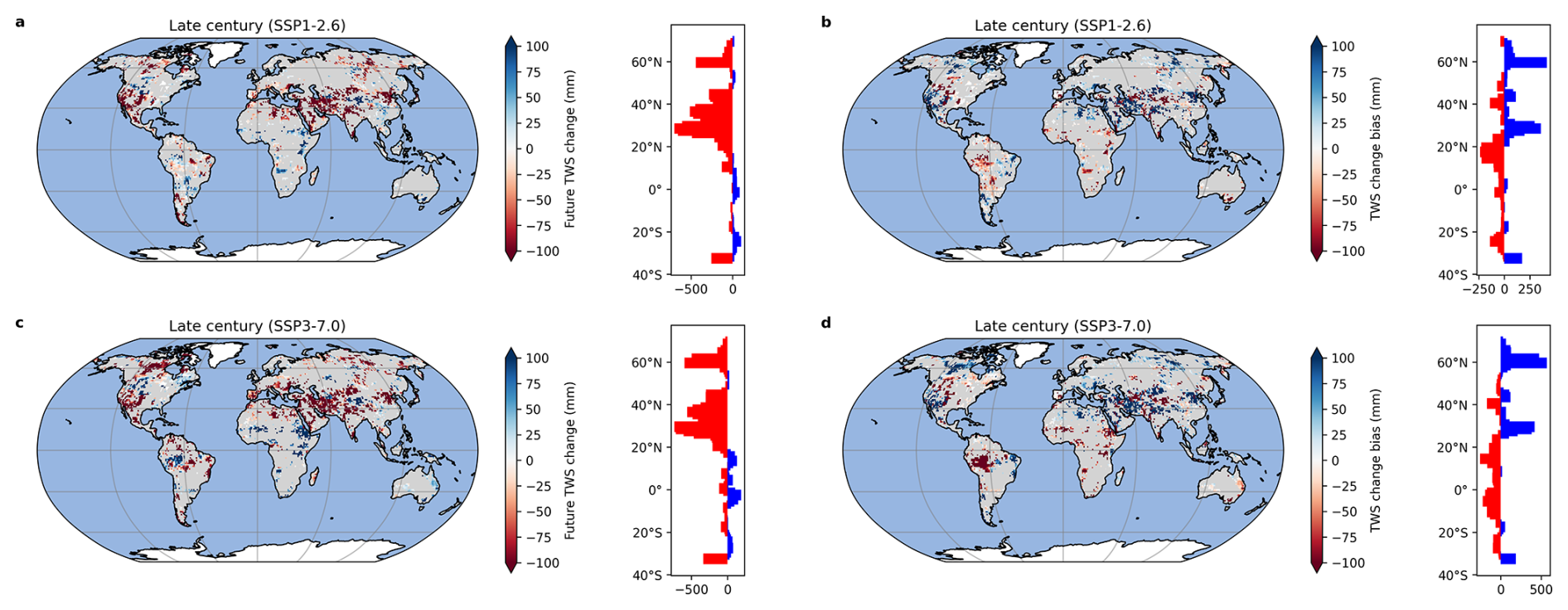
Figure 3 (a, c) Late century (2080–2099) EC-corrected TWS changes under the SSP1-2.6 and SSP3-7.0 scenarios, shown relative to historical (2004–2023) climatologies. (b, d) Biases in projected late century TWS changes (raw model outputs minus EC-corrected values). Only grid cells with statistically significant positive EC correlations (R>0 and p<0.05) are shown; non-significant regions are shaded in grey. The histograms on the right represent zonally averaged values, with data shown only for latitudes between 70° N and 35° S due to sparse coverage outside this range.

To provide accurate regional-scale projections of future TWS changes, we obtained EC-corrected maps (Fig. 3a, c) by calibrating the ISIMIP3b outputs against observed historical climatologies at each grid cell (Methods). The proposed EC correlations are robust (R>0 and p<0.05) across ∼ 26 % of global land areas (excluding Greenland and Antarctica) under both scenarios, based on the ISIMIP3b ensembles. In contrast to the raw ISIMIP3b outputs (Fig. 2a, b), the EC-corrected maps show similar patterns, such as pronounced TWS declines in the northern midlatitudes, though with greater magnitudes under both the low- and high-emissions scenarios, as highlighted in the histograms of the latitudinal mean (Fig. 3a, c). Bias patterns derived from the ISIMIP2b ensembles align with those from their ISIMIP3b counterparts, with the agreement particularly evident in the latitudinal-mean distributions (Fig. S3). The similarity in spatial patterns between the raw model outputs and the EC-corrected projections, along with the bias maps (Fig. 3b, d), corroborates our global analysis: observation-constrained TWS changes (ensemble mean) shift away from zero after the EC correction (Fig. 1). Under both emissions scenarios, the ISIMIP3b outputs notably overestimate TWS across mid- and high latitudes in the Northern Hemisphere, including regions such as the Northwest Territories in Canada, the Southwestern United States, much of the Middle East, the Danube River Basin, Siberia, and North China. Particularly, the zonal-mean TWS is overestimated by over 300 mm near 30 and 60° N under the SSP1-2.6 scenario, with an even larger overestimation exceeding 400 mm at the same latitudes under the high-emissions scenario. This overestimation is consistent with previously reported underestimations of decreasing TWS trends in models over Northern Hemisphere river basins compared to satellite observations (Scanlon et al., 2018), which may consequently lead to overestimated projections of future freshwater availability in these regions. Conversely, considerable underestimations of TWS occur in the Amazon and the Murray Basin in southeastern Australia, aligning with models' tendency to underestimate increasing TWS trends in humid regions or nonirrigated basins (Scanlon et al., 2018).

3.3 Underlying physical processes of the emergent relationship

It is crucial to elucidate the physical mechanisms linking historical and future variability in the EC relationship (Caldwell et al., 2014; Hall et al., 2019; Schlund et al., 2020). Under the SSP3-7.0 scenario, significant positive inter-model correlations (p<0.05) are found between local precipitation and TWS changes over most regions globally (Fig. 4a). Similarly, positive correlations are evident between local precipitation and other TWS-related variables, such as evapotranspiration and total runoff (Fig. 4b, c). These results are consistent with established physical understandings, affirming that local precipitation changes strongly correlate with TWS changes. More importantly, they suggest that models projecting higher precipitation changes tend to predict larger TWS increases. This finding highlights the transfer of the “wet-gets-wetter” atmospheric response to warming into future hydrological projections through precipitation forcing. Actually, climate models predicting higher warming trends often anticipate greater precipitation increases as a result of thermodynamics (Emori and Brown, 2005; Shiogama et al., 2022). At local scales, atmospheric warming-induced increases in water vapor enhance precipitation in wet regions and reduce it in dry regions (Chou et al., 2013; Held and Soden, 2006).

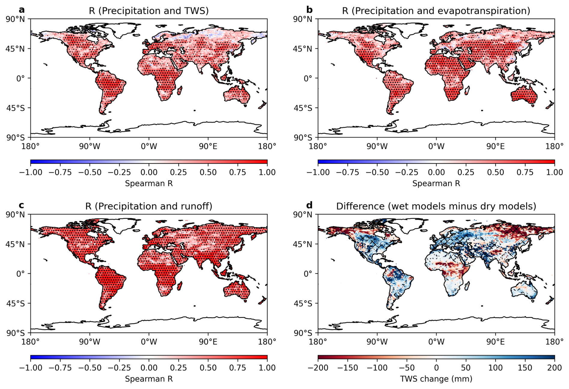
Figure 4 Inter-model Spearman's rank correlations between late century (2080–2099) precipitation changes and changes in TWS (a), evapotranspiration (b), and total runoff (c) under the SSP3-7.0 scenario. Black stippling marks regions of statistical significance (p<0.05). (d) Differences in late-century TWS changes (the wettest minus the driest models). Black hatches indicate statistically significant differences at the 5 % level, as determined by Welch's t-test. A permutation test with 100 random permutations was conducted to estimate the p-values.

Positive inter-model correlations between changes in TWS and changes in other variables, such as evapotranspiration and runoff, are found across most global land areas (Fig. S8a, b), likely reflecting the dominant influence of precipitation. After controlling for precipitation, however, partial Spearman's correlations reveal a noticeably different pattern, in particular for evapotranspiration–TWS relationships (Fig. S8c), which become negative over much of the land areas. This result indicates that enhanced evapotranspiration accelerates the depletion of future TWS, a process consistently captured by GHMs and LSMs. Conversely, the partial correlations between runoff and TWS closely resemble the original correlations even after controlling for precipitation (Fig. S8d). The widespread positive partial correlations underscore the role of high wetness and water storage in regulating runoff generation, including groundwater-driven baseflow and saturation-excess runoff (Dunne and Black, 1971; Li et al., 2025; Penna et al., 2011; Spence et al., 2010), whereby regions with greater water storage tend to produce more runoff because their buffering capacity is limited.

To further explore inter-model variations, we examine differences in TWS-related variables between the wettest and driest ensemble members based on their historical climatologies of TWS anomalies (Fig. 1, horizontal axis values; Methods). Significant differences in future TWS changes emerge, particularly in northern midlatitudes such as North America and Europe, where the driest ensemble members predict substantially lower TWS and reduced precipitation compared to the wettest ones (Figs. 4d and S4). Similar patterns of inter-model correlations and associated precipitation changes are also found under the SSP1-2.6 scenario (Figs. S5 and S6). To assess the sensitivity of our classification approach, we additionally applied the 35th and 65th percentile thresholds and found that the results are robust to the choice of threshold under the SSP3-7.0 scenario (Fig. S11).

Under the ISIMIP3b framework, the wet–dry classification aligns primarily with hydrological model structure rather than the driving climate forcing: MIROC-INTEG-LAND and WaterGAP2-2e consistently emerge as dry models, while the remaining models are classified as wet (Table S1). This structural dependence is illustrated by cases where the same climate forcing produces contrasting responses across GHMs/LSMs. For instance, MPI-ESM1-2-HR yields a wet response when driving CWatM and JULES-W2, but a dry response when coupled with MIROC-INTEG-LAND and WaterGAP2-2e. One possible explanation is that MIROC-INTEG-LAND, as a land surface model, represents subsurface hydrology with more limited deep groundwater storage compared to dedicated hydrological models (Yokohata et al., 2020). WaterGAP, while including multiple storage compartments (e.g., soil, groundwater, lakes, and wetlands), employs a relatively simplified vertical structure, lacking explicit representation of deep groundwater layering, and therefore exhibits less storage complexity than fully physically-based hydrological models (Müller Schmied et al., 2021, 2024). It is worth noting that the classification of MIROC-INTEG-LAND and WaterGAP2-2e as dry models does not imply poor performance in their historical simulations. In fact, the driest models produce present-day global mean TWS anomalies that closely match those derived from GRACE mascon solutions, whereas the wettest models tend to overestimate the historical climatology (Fig. S1).

4 Discussion

While the proposed EC relationship in Fig. 1 appears robust at the global scale, showing a high and statistically significant correlation, substantial uncertainty remains at regional scales. In particular, significant EC correlations are found over only ∼ 26 % of global land areas (Fig. 3). Regions where the proposed EC relationship does not hold include large portions of high-latitude regions such as northwestern Canada and Siberia, as well as central Asia, the Middle East, central Africa, the Amazon basin, and central Australia. These regions largely overlap with data-sparse or climatically extreme areas. There are two possible explanations for this pattern. First, as discussed earlier, the “wet-gets-wetter” responses are sensitive to the choice of study periods and regions. As a result, the signal may be attenuated in the regions with intricate hydrological processes, particularly where nonlinear land surface feedbacks, such as groundwater depletion or vegetation responses, play a role, often in remote regions subject to climatic extremes. Second, GHMs and LSMs lack sufficient observational data to adequately constrain simulations in remote regions. This limitation may weaken or obscure the “wet-gets-wetter” signal in GHMs and LSMs, even when such a signal is present in the driving GCMs.

The EC relationship does not hold for several individual realizations, which appear as outliers in the residual plots (Fig. S9). These outliers consistently deviate from the regression-defined EC relationship across scenarios (Figs. S9 and S10). Notably, realizations driven by GFDL-ESM4 and IPSL-CM6A-LR (numbered 1, 4, 6, 7, and 8 in Fig. S9) show pronounced deviations. Such systematic departures suggest that inconsistencies in these realizations may originate from their driving GCMs, likely reflecting model-specific biases in representing the “wet-gets-wetter” pattern. Furthermore, the reliability of proposed ECs could be compromised due to the lack of independence among climate models (Brient, 2020; Caldwell et al., 2014). Climate models are frequently derived from one another (Knutti et al., 2013). This challenge becomes more pronounced in future hydrological projections. LSMs and GHMs often share structural similarities in simulating water storage compartments and human water use sectors (Telteu et al., 2021). For example, all ISIMIP2b models included in this study employ the same DDM30 drainage direction map to characterize surface water routing (Döll and Lehner, 2002). In addition, three models (CWatM, MATSIRO, and MPI-HM) use an identical formulation to calculate potential evapotranspiration; while four models (CWatM, JPJmL, PCR-GLOBWB, and WaterGAP2) rely on the same set of variables to calculate changes in canopy water storage (Telteu et al., 2021). These findings underscore the critical need to ensure diversity in global models as well as in their climate forcings, particularly in water-resources-focused projects like the ISIMIP. Model selection should prioritize inclusion of models with distinct formulations of key hydrological processes and encourage integration of independently developed models such as dynamic global vegetation models alongside GHMs and LSMs. Incorporating a broad range of GCM forcings to drive all GHMs and LSMs would allow a more robust evaluation of how sensitive projections are to external climate drivers.

Several limitations should be acknowledged in this study. First, the GRACE products used in the analysis originate from a single observational system and therefore are likely affected by the same systematic biases. Second, the applicability of the EC technique is inherently limited by the knowledge space represented by the ensemble of climate models (Hall et al., 2019). If key physical processes are oversimplified or absent in the models, the EC method cannot identify or constrain those processes. Thus, the inter-model spread captured by the EC relationship may be unrealistic or unjustified due to the lack of a sound physical basis. In addition, the EC approach relies on statistical assumptions, including the stationarity of present-day relationships under future climate conditions, which may not hold and can lead to overconfident constraints (Brient, 2020; Hall et al., 2019).

In conclusion, our observation-constrained results highlight that warming-induced reductions in TWS translate into diminished freshwater availability on both global and regional scales. This is especially evident in mid- and high-latitude regions of the Northern Hemisphere, where low historical climatologies are prevalent. Our constrained estimates of global mean TWS change are roughly 83 mm lower than the raw ISIMIP3b projections, far exceeding the observed historical range of global mean TWS anomalies relative to the 2003–2020 mean (−15 to 16 mm) (Rodell et al., 2024). This large discrepancy reveals a significant overestimation of future water availability in both GHMs and LSMs. Consequently, current water resource planning may underestimate potential shortages, especially as uneven water gaps are projected to widen under warming scenarios (Rosa and Sangiorgio, 2025). Accordingly, there is an urgent need to reduce model uncertainties through robust observational constraints and enhance diversity among GHMs and LSMs, thereby improving the reliability of future hydrological projections for informed water resource management and climate adaptation.