On combining climate models into weighted ensembles

Several methods have been proposed and used to refine estimates of future climate change based on combined output from comprehensive climate models. While previously the so-called model democracy approach was used to combine model outputs, where every model is given equal weight, it is now widely accepted that using model weights that account for model performance and model independence is necessary to obtain more reliable results. However, most existing approaches rely, implicitly or explicitly, on a similar statistical basis, while describing things in different ways. Here we distinguish between approaches that are based on the performance of individual models (individual performance weighting) and approaches that are based on the performance of the weighted ensemble as a whole (ensemble performance weighting). At the same time, we formulate both in probabilistic Bayesian terms to make their application and comparison straightforward. Using simple constructed examples, we demonstrate that the ensemble performance weighting approach implicitly accounts for co-dependencies among models, which arguably makes the computation of independence weights for the purpose of model weighting obsolete. We also show that a set of weighted models within the ensemble weighting approach will naturally tend to artificially reduce uncertainty and that this is strongly influenced by the choice of the prior distribution over weight vectors. The distinction between individual and ensemble performance weighting is both methodological and conceptual. Formulating both approaches in general probabilistic Bayesian terms as done here, can serve as a common basis for future developments with regard to ensemble model weighting in Earth system science. The discussed concepts are generally applicable across domains and are thus possibly relevant for other modeling communities as well.

1 Introduction

For many decades, climate models have been an important tool for gaining a better understanding of the climate system, and for making inferences about future climate and the consequences of climate change. Over the years many different models have become available which is generally beneficial to get a more accurate picture of reality. There are, for instance, different possibilities on how to parameterize processes that cannot be resolved in the models, which leads to uncertainties in the simulated data that can be represented by using an ensemble of models. This type of uncertainty is referred to as model- or structural uncertainty, and it is the primary uncertainty addressed by a multi-model ensemble. In the most straightforward way, each model in an ensemble is considered equally important and thus receives equal weight. This is therefore known as the “model democracy” approach, where simple multi-model means (MMMs) are computed and the ensemble spread is used to quantify uncertainty. While this has long been the standard approach, it comes along with several problems that can be addressed by weighting the models in the ensemble.

A general challenge is that we must work with “ensembles of opportunity”: the available models do not represent a statistically perfect ensemble in the sense of a set of unbiased and independent random samples (e.g., see Masson and Knutti, 2011; Pennell and Reichler, 2011). They were not constructed to cover the entire range of plausible outcomes, nor is this space evenly sampled as the models can be dependent on one another in complex and often intransparent ways. Due to such inter-model dependencies, they may, for instance, have shared biases, which essentially means that some models in the ensemble do not provide as much new information as others (e.g., see Jun et al., 2008). Furthermore, the models may differ in how plausible they are in light of the observational data. Therefore, there are two main aspects that weights assigned to models in an ensemble should account for: model performance and model dependence.

Various methods have been proposed in the literature to compute model weights that reflect one or both aspects. A method that has received much attention is ClimWIP from Brunner et al. (2020), which was developed from a long line of previous work (e.g., Sanderson et al., 2015b, a; Knutti et al., 2017; Lorenz et al., 2018). It combines weights that are calculated separately for independence, defined in terms of model output similarities, and performance. Both types of weights are computed based on the assumption of a Gaussian error model and by taking one or more diagnostic variables into account. The diagnostic variables used for computing performance weights may be different from those used to calculate independence weights. Meanwhile, the Reliability Ensemble Averaging method (REA) is a similar method introduced by Giorgi and Mearns (2002) which also considers model performance and independence. Another, conceptually different approach is what is often referred to as Bayesian Model Averaging (BMA). While the other methods mentioned above compute model weights based on the performance and/or independence of the individual models in the ensemble, BMA-weights are based on the performance of the weighted ensemble itself. Therefore, the BMA-weights are selected so that the weighted average model simulates the observed data as closely as possible (e,g. Massoud et al., 2020; Wootten et al., 2020; Massoud et al., 2023; Wootten et al., 2023). It should be noted that this definition of BMA differs from what BMA refers to in the context of statistical models where it was first applied, but since the application of BMA on forecasting surface temperatures by Raftery et al. (2005), it has become a common way to refer to the method used in at least some climate science studies today.

Although the methods differ in the details, they can mainly be distinguished by whether the ensemble is considered as a whole, which we will refer to as “Ensemble Performance Weighting”, or as individual members, which we will refer to as “Individual Performance Weighting”. All approaches to computing model weights have in common that they need to provide answers to the following two questions: (i) how to compute model performance and (ii) how to account for potential dependencies between models. Concerning model performance, Sierra and Muñoz (2025), for instance, use a method, embedded in information-theoretic concepts, that computes performance weights relative to the inverse of the deviations between model output and data. Similarly, Feng et al. (2011) use inverse-distance power weighting $(\frac{\mathrm{1}}{{\mathrm{AE}}_i^r}$, r>0, AE_i: absolute error of model i) to compute performance weights. Others define performance based on the assumption of independent and identically distributed Gaussian errors (e.g.  Brunner et al., 2020). Note that all such individual-performance weighting approaches where the weights are a function of the sum of squared errors yield the same ranking order, only the magnitude of the weights differs (see Appendix B for examples).

Meanwhile, independence is often defined in terms of model similarities (e.g. see Brunner et al., 2020). The more similar the output of two models is, the more dependent they are considered to be. This is reasonable in that two dependent models will have shared biases which is reflected in similar model output for both. Another option is to use meta information about the climate models that could provide further insights about co-dependencies between the models, e.g., information about the modeling group, specific model components or model resolution (e.g. see Boé, 2018; Kuma et al., 2023). However, contrary to the model output, this information is not always available, making model similarities a pragmatic choice to define model independence. Furthermore, even if meta information about the models were available, there would not be a unique straightforward definition of independence. As pointed out by Massoud et al. (2023), considering full distributions over weight vectors rather than a single weight per model implicitly provides information about inter-model dependencies. The idea is that this is due to the correlation between the posterior weights of different models. This is an important claim that is fundamental to the distinction between “individual” performance weighting and “ensemble” performance weighting.

Here we aim to clearly define these two approaches within the common language of probabilities in Bayesian terms, so that we can easily compare and apply both methods in a consistent way. We use simple, idealized examples to test the methods in a systematic way, with a particular focus on the question of how inter-model dependencies are accounted for in a model weighting exercise. We also explore how the results obtained from applying this approach are affected by different methodological choices about the prior distribution over weights, which can be important and should be a prominent aspect of the ensemble performance weighting approach.

The paper is structured as follows. In Sect. 2 we lay out the differences between the two approaches and define the terminology we use. In Sects. 3 and 4, we discuss choices for the prior and likelihood distributions and consider the influence of using a set of different diagnostic variables, including a simple example. In Sect. 5 we consider the issue of model dependence through simple examples, while in Sect. 6, we consider the particular realistic case of using Equilibrium Climate Sensitivity (ECS) as a performance diagnostic. In Sect. 7, we discuss the overall implications of our work. Section 8 concludes the paper and provides an outlook on future work.

2 Conceptual framing of weighting approaches

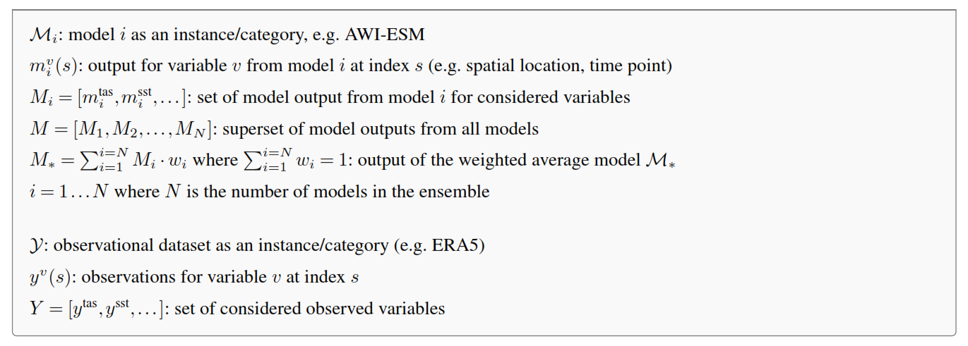
In the following we will provide definitions for the two general approaches for computing model weights, the individual and the performance weighting approach, and specify the terminology that we use throughout the paper. This is summarized in Box 1. Note that generally, lowercase letters refer to model output/observations for a specific climate variable, while uppercase letters refer to collections, e.g., of different variables or models. An exception are uppercase calligraphic letters, ℳ_i and 𝒴, which we use to refer to a model i or an observational dataset as a category.

Box 1 Terminology.

2.1 Individual performance weighting

With the individual performance weighting approach, a weight vector is defined such that each weight represents the plausibility of the respective model in light of the observed data Y. In this approach, the weight assigned to a model ℳ_i is proportional to the product of the likelihood of the observed data Y under model ℳ_i, i.e. given its output, M_i, and the prior over models, P(ℳ_i).

$$\begin{array}{}\text{(1)}& w_i\propto P\left(Y\mid M_i\right)\cdot P\left({\mathcal{M}}_i\right)\end{array}$$

When each model is a priori considered equally likely, the resulting weight vector is only influenced by the likelihood, and the prior can thus be omitted. This simplifies Eq. (1) into $w_i\propto P(Y\mid M_i)$. Note the difference between the model as a category, ℳ_i and its output M_i, where the former implies the latter: once we decide for a model (e.g. AWI-ESM), we can look up its output. Therefore, for completeness, we note that Eq. (1) can be spelled out explicitly as

$$\begin{array}{}\text{(2)}& \begin{array}{rl}{w}_i& =P\left({\mathcal{M}}_i\mid Y,M_i\right)\propto P\left(Y\mid {\mathcal{M}}_i,M_i\right)\cdot P\left(M_i\mid {\mathcal{M}}_i\right)\\ & \cdot P\left({\mathcal{M}}_i\right)=P\left(Y\mid M_i\right)\cdot \mathrm{1}\cdot P\left({\mathcal{M}}_i\right).\end{array}\end{array}$$

2.2 Ensemble performance weighting

In the ensemble performance weighting approach, the objective is to find a weight vector w so that the likelihood of the observed data is maximized under the weighted average model, ℳ_*. Thus, performance is not considered for individual models, but for the ensemble as a whole. This is the main difference between both approaches yielding two conceptually different outputs: in the individual weighting approach, we get a discrete distribution over categories (the models in the ensemble), i.e. a single weight vector whereas in the ensemble weighting approach, we get a continuous distribution over weight vectors:

$$\begin{array}{}\text{(3)}& P\left(\mathit{w}\mid Y,M\right)\propto P(Y\mid M,\mathit{w})\cdot P\left(\mathit{w}\right)=P\left(Y\mid M_{*}\right)\cdot P\left(\mathit{w}\right).\end{array}$$

For a weight vector w, the output of the weighted average model ℳ_* for a variable v is given by

$$\begin{array}{}\text{(4)}& m_{*}^v=\sum _{i=\mathrm{1}}^N{w}_i\cdot m_i^v.\end{array}$$

Thus, the log likelihood of the observed data under model ℳ_*, i.e. given its output, M_*, is computed as

$$\begin{array}{}\text{(5)}& \log P\left(Y\mid M_{*}\right)=\sum _v\log P\left(y^v\mid m_{*}^v\right).\end{array}$$

To find the weight vector associated with the maximum likelihood, stochastic sampling methods can be used. For example, using Markov Chain Monte Carlo (MCMC) sampling, we can approximate the posterior distribution over weights w (Eq. (3)). This has the advantage that uncertainties around the weights are incorporated and can thus be naturally propagated. Therefore, instead of assuming a single weight vector when computing model output (e.g., future climate projections), this approach allows us to compute a posterior predictive distribution that accounts for our uncertainty in the weights. If we want to summarize the posterior distribution over weights, we may compute the mean or the maximum-a-posteriori (MAP) weight vector. For unimodal and symmetrical distributions these two values should be nearly identical (for an overview on Bayesian data analysis see Gelman et al., 2013).

Note the difference in the interpretation of the weights in the ensemble performance weighting approach compared to the individual performance weighting approach. The mean estimates of the sampled weights (in the ensemble performance weighting approach) represent the average contribution that a model makes to the weighted average. This is not strictly equivalent to, but can be interpreted as the relative performance of each model. Contrary to that, the weights computed in the individual performance weighting approach exactly mirror the performance of each individual model compared to the other models in the ensemble.

Irrespective of the applied approach (individual or ensemble performance weighting), we need to define (i) a prior distribution and (ii) a likelihood function (i.e. P(Y∣M_i) for each model ℳ_i or $P(Y\mid M_{*}$) for the weighted average model, respectively), or more generally speaking, a way to measure model performance with respect to the observed data. We will consider both in turn in the next two sections.

3 Prior distributions

In the individual weighting approach the prior is defined over models (as categories), while in the ensemble weighting approach the prior is defined over weight vectors. In the absence of any available information about the models before considering the data, like information about model dependencies, for example, the most neutral choice for the prior is a distribution that treats each model, or in the ensemble weighting approach, each weight vector, as equally likely. In the individual performance weighting approach, this corresponds to an equal probability for each model, or $p_i=\frac{\mathrm{1}}{N}$ where N is the number models. Mathematically this is described by a categorical distribution:

$$\begin{array}{}\text{(6)}& {\mathcal{M}}_i\sim \mathrm{Categorical}\left(\mathit{p}=\left[{\displaystyle \frac{\mathrm{1}}{N}},\mathrm{\dots },{\displaystyle \frac{\mathrm{1}}{N}}\right]\right).\end{array}$$

If available, prior knowledge can be taken into account by adjusting the parameter vector p accordingly, subject to the constraint $\sum _{i=\mathrm{1}}^N{p}_i=\mathrm{1}$. Analogously, in the ensemble performance weighting approach, we draw weight vectors from a Dirichlet distribution with parameter vector α where we set each entry α_i to the same constant value c:

$$\begin{array}{}\text{(7)}& \mathit{w}\sim \mathrm{Dirichlet}(\mathit{\alpha }=[c,\mathrm{\dots },c\left]\right)\mathrm{with}c>\mathrm{0}.\end{array}$$

The Dirichlet distribution is defined over N-dimensional vectors that sum up to 1. When all α_i are identical, the vector α reduces to a single scalar α, also called the concentration parameter. Figure 1a shows the distribution of each component w_i of weight vectors drawn from a Dirichlet distribution over 3-dimensional vectors (corresponding to an ensemble of three models) and how it changes with varying α. The expected value for w_i, i.e. for model i, is given by $\frac{{\mathit{\alpha }}_i}{{\mathit{\alpha }}_{\mathrm{0}}}$ where α₀ = ${\sum }_{i=\mathrm{1}}^N{\mathit{\alpha }}_i$. Therefore, when all parameters α_i are set to the same value c, the expected value for each w_i is always equal to $\frac{\mathrm{1}}{N}$ since $E\left[w_i\right]=\frac{{\mathit{\alpha }}_i}{{\mathit{\alpha }}_{\mathrm{0}}}=\frac{c}{N\cdot c}=\frac{\mathrm{1}}{N}$. This is the case in the two bottom rows of Fig. 1a, where α=1 and $\mathit{\alpha }=\frac{\mathrm{1}}{N}$ respectively. It is, therefore, a reasonable choice to set all α_i to a single value when we do not have any prior knowledge about the models' weights. Yet, the sampled vectors differ depending on the absolute value of α: when α=1, the prior mass is evenly spread and all w_i are close to the expected value $\frac{\mathrm{1}}{N}$ whereas when α<1, the weights tend to be either large or small (U-shaped distribution). In the asymptotic case where α→0, the weight vectors approach one-hot vectors, i.e. nearly all probability mass is assigned to a single model, while all others receive almost no weight. The upper three rows of Fig. 1a further show how the distribution of each w_i changes when an exemplary basis parameter vector of [0.1, 0.4, 0.5] is multiplied by 0.1, 10 and 100 respectively. The larger the parameter values α_i are, the tighter the distributions scatter around the respective mean value. Therefore, the Dirichlet distribution allows us to easily incorporate potential prior knowledge about the value of a model's weight: the more certain we are a priori, the larger we set the value of the corresponding parameter α_i. There are alternative distributions for vectors that sum up to 1 such as the Logit Normal distribution. These were, however, not explored in this work.

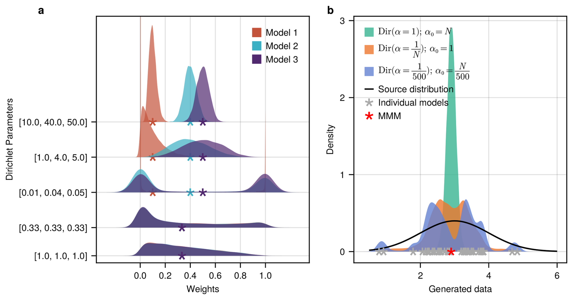
Figure 1 (a) Distributions of weights per model sampled from a Dirichlet distribution using different parameters. The stars show the mean weights. In the bottom two rows, the distributions of the individual model weights are identical, hiding the distributions for models 1 and 2 behind the distribution for model 3. (b) Artificial data (grey dots) of 38 “models”, drawn from $\mathcal{N}(\mathit{\mu }=\mathrm{3},\mathit{\sigma }=\mathrm{1})$ (black curve). The densities show the distributions of the expected data of the weighted average models computed for each of 10 000 weight vectors drawn from Dirichlet distributions with varying parameters.

Especially in cases where we only have few or not very informative data, the choice of the prior needs careful consideration as, in that case, the posterior will be more influenced by the prior. Figure 1b shows how the choice of the prior distribution over the weight vectors influences the data that is considered in the first place by the weighted average models. Here, we generated arbitrary data for 38 models (grey stars) by drawing from a Normal Distribution with μ=3, σ=1 (black curve) to represent an ensemble of opportunity. The three colored densities show the distribution of the weighted averages under Dirichlet priors (over w) with varying concentration parameter α. In all three cases, the expected value for each w_i equals $\frac{\mathrm{1}}{N}$, reflecting that we do not have any prior knowledge about the models' weights. When α=1 (green density), all weight vectors that we consider through the prior distribution assign approximately equal probability to all w_i, so that we are naturally restricted to weighted averages that sit tightly around the multi-model mean. When α is extremely small (purple density where $\left.\mathit{\alpha }=\frac{\mathrm{1}}{\mathrm{500}}\right)$, the considered “weighted” averages effectively correspond to the output of individual models as the prior distribution generates vectors that approach one-hot vectors (where α_j=1, ${\mathit{\alpha }}_i=\mathrm{0}\forall i\ne j$). Setting $\mathit{\alpha }=\frac{\mathrm{1}}{N}$ (orange density) turns out to be a reasonable choice in that the weight vectors drawn from this prior distribution allow us to cover a large part of the spread of the model ensemble. This is due to the variance of the Dirichlet distribution, with scalar concentration parameter α, defined as $\mathrm{var}\left(w_i\right)=\mathit{\lambda }\cdot \frac{\mathrm{1}}{N\cdot \mathit{\alpha }+\mathrm{1}}$ where $\mathit{\lambda }=\frac{N-\mathrm{1}}{N^{\mathrm{2}}}$, i.e. λ does not depend on α. The variance of the prior weights will therefore be very small if α does not depend on the number of models (assuming a moderate number of models, in Fig. 1b, we use N=38), even if it is set to a small value like 1. And since a small variance in the prior weights yields a highly homogeneous set of weight vectors that are considered in the first place, the data that is a priori considered by the weighted average models is restricted accordingly.

In summary, in the individual performance weighting approach, a uniform prior over the models will likely be the best choice in most cases, unless one has prior knowledge that justifies to prefer certain models over others. In the ensemble weighting approach, the prior should be considered more carefully as there are several choices with quite different implications even if we assume no prior knowledge, reflected by an expected value for each w_i of $\frac{\mathrm{1}}{N}$. In this case, $\mathit{\alpha }=\frac{\mathrm{1}}{N}$ seems to be a good choice.

4 Measuring performance

The choice of how to evaluate model performance lies at the heart of every method to compute weights for models in an ensemble. For data on a spatial grid, an example for a performance metric f is the inverse mean squared error between model output and observed data:

$$\begin{array}{}\text{(8)}& f\left(m_i^v,y^v\right)={\displaystyle \frac{\mathrm{1}}{\sum _s{w}_s\cdot {\left(m_i^v\left(s\right)-y^v\left(s\right)\right)}^{\mathrm{2}}}}\end{array}$$

where s iterates over spatial locations and w_s refers to weights (such as area weighting) normalized to sum to 1.

In the individual performance weighting approach, the weight for model i is then proportional to the performance of model i, based on performance metric f, and assuming a uniform prior over models here for simplicity.

$$\begin{array}{}\text{(9)}& w_i\propto f\left(m_i^v,y^v\right)\end{array}$$

This approach was, for instance, used by Sierra and Muñoz (2025). To formulate the weighting in a Bayesian framework, we need to define a proper generative likelihood function instead of relying on a heuristic performance metric. The likelihood relates model output to the observed data in a probabilistic way and allows us to incorporate uncertainties that are not accounted for when using a heuristic performance metric. A possible choice for the likelihood is to assume independent and identically distributed (i.i.d.) Gaussian errors so that

$$\begin{array}{}\text{(10)}& {\displaystyle }& {\displaystyle }{y}^v=m_i^v+\mathit{ϵ},\mathit{ϵ}\sim \mathcal{N}\left(\mathrm{0},{\mathit{\sigma }}^{\mathrm{2}}\right)\text{(11)}& {\displaystyle }& {\displaystyle }{y}^v\sim \mathcal{N}\left(m_i^v,{\mathit{\sigma }}^{\mathrm{2}}\right)\end{array}$$

where m_i refers to the output of any model ℳ_i, be it from a weighted-average model or an individual model. Assuming i.i.d. errors is often unrealistic, but is commonly used as a convenient simplification. The performance weights as computed with ClimWIP (Brunner et al., 2020) are an example of assumed Gaussian errors using individual performance weighting, while Massoud et al. (2020), for instance, use Gaussian errors with ensemble performance weighting. Using Gaussian errors requires choosing a value for the variance, σ². In the individual performance weighting approach, σ² acts as a hyperparameter that regulates the strength of the relative weighting between models: the smaller σ², the fewer models are considered to simulate the observed data well. Thus, the number of models that are assigned weights substantially greater than 0 decreases with decreasing σ². For ClimWIP, Brunner et al. (2020) tune a parameter (σ_D) that essentially represents the variance σ², with the objective to obtain a weighting that is neither too weak (all equal) nor too aggressive (all weight on few models only). As an objective measure of where this value should be, Brunner et al. (2020) follow Knutti et al. (2017) and run perfect model tests with different values for σ_D. They then set σ_D to the smallest value such that more than 80 %, (90 % in Knutti et al., 2017) of the perfect models lie in the 10 %–90 % (5 %–95 % in Knutti et al., 2017) range predicted by weighting all but the respective “perfect” model. Note, that the ranking of which models are best remains the same irrespective of σ²; only the magnitudes of the weights change. In ClimWIP, the performance weight of a model i is proportional to the likelihood of the observed data under a Gaussian distribution:

$$\begin{array}{}\text{(12)}& w_i\propto \mathcal{L}\left(y\mid \mathit{\mu }=m_i^v,{\mathit{\sigma }}^{\mathrm{2}}={\displaystyle \frac{{\mathit{\sigma }}_D^{\mathrm{2}}}{\mathrm{2}}}\right)\cdot P\left({\mathcal{M}}_i\right).\end{array}$$

In general, it is also possible to sample σ², which would make the tuning procedure like it was done by Brunner et al. (2020) unnecessary. However, with ClimWIP, or the individual performance weighting approach in general, this would simply result in a nearly equal weighting since σ² would be tuned to increase the likelihood of the observed data under every model. Contrary to that, in the ensemble weighting approach, this problem does not arise as the posterior over σ² represents our uncertainty across the weighted-average models, so that there is no direct relation between the individual model weights and σ². A common prior distribution for the unknown variance of a normal distribution is, for instance, the inverse-gamma distribution (e.g., see Gelman et al., 2013, Chapter 2.6), which we also use in the examples in the following sections where we apply the ensemble performance weighting approach. The joint posterior distribution over weight vectors and variance σ² is then given by:

$$\begin{array}{}\text{(13)}& P\left(\mathit{w},{\mathit{\sigma }}^{\mathrm{2}}\mid M\right)\propto \mathcal{L}\left(y\mid \mathit{\mu }=m_{*}^v,{\mathit{\sigma }}^{\mathrm{2}}\right)\cdot P\left(\mathit{w}\right)\cdot P\left({\mathit{\sigma }}^{\mathrm{2}}\right)\end{array}$$

where $m_{*}^v$ is the output for variable v of the weighted average model using weight vector w. Setting σ² to a fixed value in the ensemble weighting approach is also an option. Massoud et al. (2020), for instance, use the following log likelihood function: $-\frac{\mathrm{1}}{\mathrm{2}}\sum _s\left(Y\right(s)-M_i(s){)}^{\mathrm{2}}$, where s iterates over all grid cells¹, which is equivalent to assuming Normal Gaussian errors centered around 0 with variance σ²=1.

4.1 Measuring performance based on a set of diagnostics

In the previous section, we focused on a single diagnostic v. This could, for instance, be the temperature anomaly of a specific time period. In this section, we want to consider the case when the performance weights are based on more than one diagnostic. There are generally two approaches: either the weights are computed separately for each diagnostic and are then averaged to yield a final weight vector or the different diagnostics are considered all at once. In the ClimWIP-method (individual weighting) for example, Brunner et al. (2020) compute one distance value for every model across a set of five different diagnostics. To make the diagnostics unitless, that is, to bring them all on the same scale, they normalize the distance value for each model by the median across all models, respectively for every diagnostic. The normalized distances are summed up for every model so that eventually each model is assigned one “generalized” distance value. Performance weights are then based on a Gaussian distribution over these values. In this way, the diagnostics are considered together. An alternative example for using several diagnostics, yet in the ensemble weighting approach, is the study from Massoud et al. (2020), who compute one weight vector separately for each diagnostic and then take the average across all computed weight vectors.

Figure 2 Generated toy data for two models and diagnostics so that model 1 is the objectively better model. All data were normalized by the standard deviation of the corresponding observations. The grey lines show the 1:1 perfect matches. (a) Diagnostic 1 with $m_{\mathrm{1}}^{\mathrm{tas}}=y^{\mathrm{tas}}+\mathcal{N}(\mathrm{0},s_{\mathrm{tas}})$ and $m_{\mathrm{2}}^{\mathrm{tas}}=y^{\mathrm{tas}}+\mathcal{N}(\mathrm{0},\mathrm{3}\cdot s_{\mathrm{tas}})$. (b) Diagnostic 2 with $m_{\mathrm{1}}^{\mathrm{psl}}=y^{\mathrm{psl}}+\mathcal{N}(\mathrm{0},\mathrm{1.5}\cdot s_{\mathrm{psl}})$ and $m_{\mathrm{2}}^{\mathrm{psl}}=y^{\mathrm{psl}}+\mathcal{N}(\mathrm{0},s_{\mathrm{psl}})$. The standard deviations for the noise were set to $s_{\mathrm{tas}}=\mathrm{2},s_{\mathrm{psl}}=\mathrm{90}$.

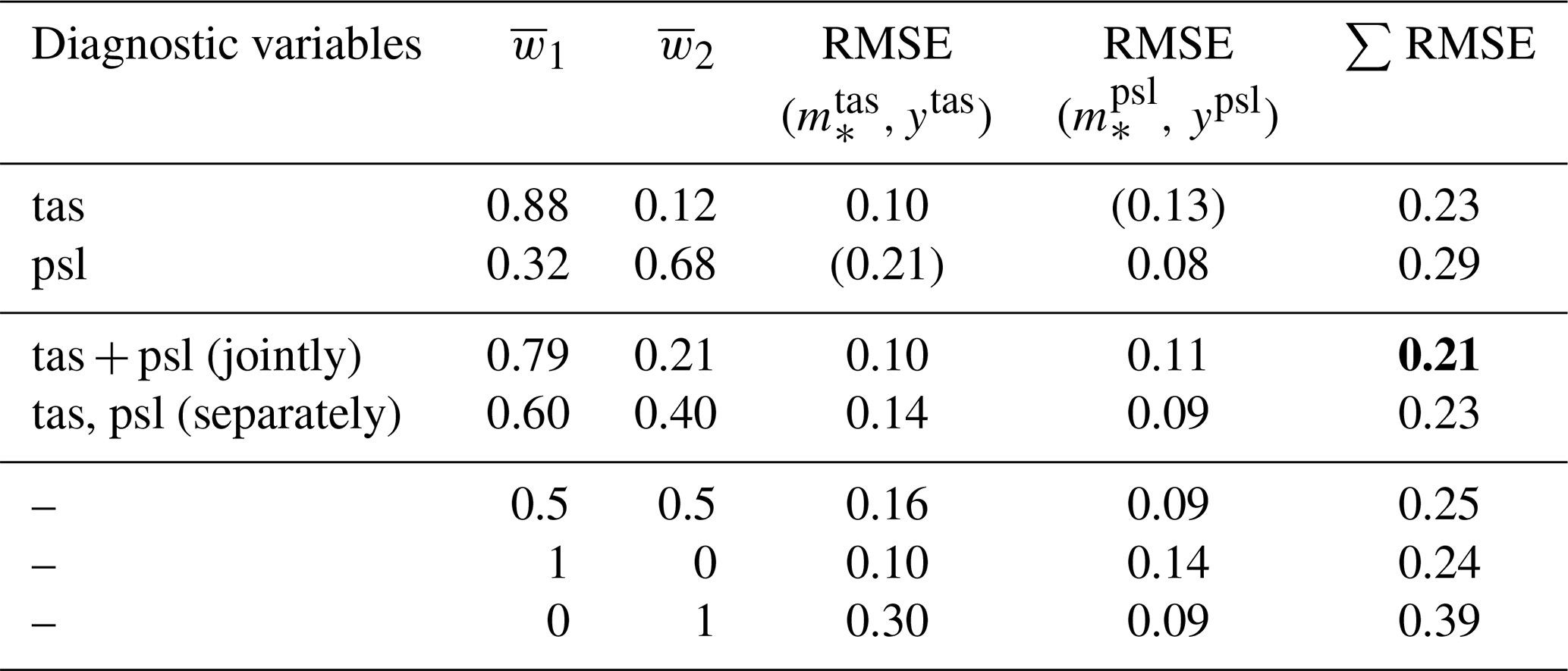
Table 1 Mean posterior weights (columns 2 and 3, values are rounded) with RMSEs for the corresponding weighted average model, using the constructed data from Fig. 2. The RMSEs for the diagnostics that were not used in the objective function are put in parentheses (columns 4 and 5). Note the weight vector in row 4 (tas,psl separately) corresponds to $\frac{w^{\mathrm{tas}}+w^{\mathrm{psl}}}{\mathrm{2}}$, i.e. it is not sampled, but the average of weight vectors in rows 1 and 2, where each diagnostic was considered independently. For comparison, row 5 shows the RMSEs for the multi-model mean and the last two rows show the RMSEs when relying on individual models, using either model 1 or model 2. The overall smallest summed RMSE is highlighted in bold.

To show the implications of this choice – i.e. whether to compute one distribution of weights for every diagnostic or a single distribution of weights that takes into account all diagnostics at once – we generated toy data for two models and two diagnostics, shown in Fig. 2. The data that we use here are anomalies of climatologies for the time period from 1980–2014 with respect to the global mean value. For diagnostic 1, we use near surface air temperature (tas) and for diagnostic 2, we use sea level pressure (psl). To bring the data of both diagnostics on the same scale, we standardize them by the standard deviation of the observations (ERA5) for the respective diagnostic. The toy model data were constructed so that for diagnostic 1, ℳ₁ is much better than ℳ₂, while for diagnostic 2, ℳ₂ is better than ℳ₁, albeit only marginally (see Fig. 2). In this way, ℳ₁ is objectively the better model and thus, when both diagnostics are taken into account at the same time, we expect ℳ₁ to receive larger weights on average than ℳ₂. Nonetheless, as ℳ₂ performs better for diagnostic 2 than ℳ₁, it should still payoff to include ℳ₂ to some extent in a weighted average than relying only on ℳ₁ alone.

To compute the posterior distributions over weight vectors, we use a Dirichlet prior parameterized with $\mathit{\alpha }=\left[\frac{\mathrm{1}}{\mathrm{2}},\frac{\mathrm{1}}{\mathrm{2}}\right]$ and a multivariate Gaussian likelihood with the models' outputs as mean vector and variances ${\mathit{\sigma }}_{d_{\mathrm{1}}}^{\mathrm{2}}$, ${\mathit{\sigma }}_{d_{\mathrm{2}}}^{\mathrm{2}}$ for diagnostic 1 and 2 respectively that we sample jointly with the weights. Note that the values for the variances are not reported further, as they are not relevant to the result. The results summarized in Table 1 confirm our expectations: when both diagnostics are jointly used, the mean weight vector is $\langle {\stackrel{\mathrm{‾}}{w}}_{\mathrm{1}}=\mathrm{0.79},{\stackrel{\mathrm{‾}}{w}}_{\mathrm{2}}=\mathrm{0.21}\rangle >$, giving more weight to model ℳ₁ than to model ℳ₂. Also, the summed RMSE for the corresponding weighted average model is smaller (0.21) than it is when using the first model alone (0.24) because of the reduced RMSE for diagnostic 2 (0.11 vs. 0.14) that results from giving some weight also to model ℳ₂.

When instead, both diagnostics are considered separately, i.e. we first compute the posterior distributions over weight vectors, one based on diagnostic 1, the other based on diagnostic 2, and then average the resulting mean posterior weights, we get a mean weight vector of $\langle {\stackrel{\mathrm{‾}}{w}}_{\mathrm{1}}=\mathrm{0.6},{\stackrel{\mathrm{‾}}{w}}_{\mathrm{2}}=\mathrm{0.4}\rangle$, thus reducing the weight assigned to model ℳ₁ compared to the joint case. With this weight vector, the summed RMSE is larger (0.23) than it is when using both diagnostics jointly (0.21), yet still smaller than when using only model ℳ₁ (0.24).

This example shows that, when possible, it is better to consider all diagnostics simultaneously to obtain more representative weight vectors.

Figure 3 Generated toy data with same error pattern for both models. (a) Observations, near-surface air temperature anomalies in the time between 1980 and 2014 with respect to the global mean value of this time period. (b) $M_{\mathrm{1}}\left(s\right)=Y\left(s\right)+\mathcal{N}(\mathrm{0},\mathrm{2})$ where s is a grid point in the Western hemisphere. For all s in the Eastern hemisphere, the output of model 1 is identical to the observations. (c) Output of model 2, with identical errors as for model 1, yet in the Eastern hemisphere, while the Western hemisphere is identical to the observations.

Figure 4 Generated toy data with independent noise per model. (a) Observations, near-surface air temperature anomalies in the time between 1980 and 2014 with respect to the global mean value of this time period. (b) $M_{\mathrm{1}}\left(s\right)=Y\left(s\right)+\mathcal{N}(\mathrm{0},\mathrm{2})$. (c) Output of model 2, analogous to model ℳ₁, but with independently sampled noise.

Figure 5 Observations of near-surface air temperature anomalies in the time between 1980 and 2014 with respect to the global mean value of this time period (a) and corresponding output of two real models, AWI-CM-1-1-MR (b) and CESM2-WACCM (c).

5 Model dependence

We would like to use three schematic (toy) examples to illustrate how the possible lack of independence between ensemble members can influence the weights obtained when using individual or ensemble performance weighting. In each case, we use an ensemble of two base models, ℳ₁ and ℳ₂, whose output is systematically constructed based on the 1980–2014 mean near-surface air temperature anomalies with respect to the global mean, obtained from ERA5 (Hersbach et al., 2020).

In the first case, we assume that the first model (ℳ₁) perfectly simulates the Eastern Hemisphere, while in the Western Hemisphere, a random error sampled from 𝒩(0,2) is added to the field. For the second model (ℳ₂), the same random error is added in the Eastern Hemisphere, while the Western hemisphere is perfectly simulated. In this way, we get two models with the exact same mean squared error (MSE) with respect to the observed data and we know that the weighting that would minimize the total combined error would be $w_{\mathrm{1}}=w_{\mathrm{2}}=\mathrm{0.5}$. The data for this case are shown in Fig. 3.²

In the second case, we set the output of the two models everywhere to the observed data and independently add the noise to both models (again sampled from 𝒩(0,2)). Therefore, in this example, the mean squared errors will be similar, but are very unlikely to cancel out at every grid point. The constructed data for this case are shown in Fig. 4.

In the third example, we do not construct data, but use the output for the same variable and diagnostic from two real models, namely from AWI-CM-1-1-MR and CESM2-WACCM. These data are shown in Fig. 5.

Figure 6 Model weights for models in an ensemble consisting of model ℳ₁ and n₂ copies of model ℳ₂. Panels (a)–(c) show the computed weights in the individual performance weighting approach, panels (d)–(f) show the mean posterior weights in the ensemble performance weighting approach. Columns refer to the three different toy examples. Toy example 1 (a, d): ℳ₁ and ℳ₂ predict one half of the data perfectly and show the same bias (𝒩(0,2)) in the other half. Toy example 2 (b, e): model outputs are constructed from the observed data plus some random noise everywhere: $m_i=y+\mathit{ϵ}$ where $\mathit{ϵ}\sim \mathcal{N}(\mathrm{0},\mathrm{2})$. Toy example 3 (c, f): ℳ₁ and ℳ₂ correspond to AWI-CM-1-1-MR and CESM2-WACCM. The two values in brackets in the titles are the mean squared errors for models ℳ₁ and ℳ₂ in the respective example.

In each of the three toy examples described above, we build ensembles of different sizes by adding copies of model ℳ₂. We know that, by construction, the weight of model ℳ₁ (included just once) should always have the same value, irrespective of the number of copies of model ℳ₂ included in the ensemble (and conversely, the sum of weights attributed to the included copies of model ℳ₂ should be equal to the constant value 1−w₁). In the first toy example, both models have the exact same performance (same MSE) so that the weight for ℳ₁ should remain at $\frac{\mathrm{1}}{\mathrm{2}}$, while the individual copies of model ℳ₂ should each receive a weight of $\frac{\mathrm{1}}{\mathrm{2}}\cdot \frac{\mathrm{1}}{n_{\mathrm{2}}}$ where n₂ is the number of included copies for ℳ₂. The same pattern should apply to the other two toy examples, but with the weight for ℳ₁ remaining at whatever value it receives when model ℳ₂ is included in the ensemble only once. In the second toy example, where we use random errors, this should still be close to $\frac{\mathrm{1}}{\mathrm{2}}$ whereas in the third example with real model data it depends on how much better or worse ℳ₁ is compared to ℳ₂. In the case that the model weights deviate from these expectations, it implies that the known (strong) dependence between the copies of model ℳ₂ is not properly accounted for.

Figure 6 shows the resulting weights for these toy examples, using individual or ensemble performance weighting. In the individual performance weighting approach, we evaluate the models by their MSEs (identical to using the sum of squared errors). In the ensemble performance weighting approach, we use a Gaussian likelihood function with the variance jointly sampled with the weight vectors; the shown weights are the mean posterior weights. For the prior over weight vectors, we use a Dirichlet distribution with ${\mathit{\alpha }}_i=\frac{\mathrm{1}}{N}\forall i$ where N is the respective total number of models in the considered ensemble.

In the individual weighting approach, the weights for model ℳ₁ decrease as N increases, essentially following the relationship $w_{\mathrm{1}}=\frac{\mathrm{1}}{N}$. In this case the weight given to any individual copy of model ℳ₂ follows the same relationship. This means that the total weight assigned to ℳ₂ increases to $\frac{N-\mathrm{1}}{N}$. Conversely, in the ensemble weighting approach, neither the weight for model ℳ₁ nor the summed weight across all copies of model ℳ₂ changes with increasing N. Thus, only the ensemble weighting approach is able to account for the dependencies among the models in the ensemble that we introduced by adding copies of model ℳ₂ to the ensemble. When performance is measured for the entire ensemble, adding copies of one model does not have an effect on the mean weights since no new information is added. In the individual weighting approach, a newly added copy, however, is seen to add information to the ensemble by definition as every model is considered separately. Implicitly accounting for model dependence is a strong advantage of the ensemble weighting approach, making the additional computation of independence weights unnecessary. Nonetheless, in the individual weighting approach, it is possible to combine performance and separately determined independence weights so that the weight of dependent models is reduced (e.g. see tests from Brunner et al., 2020).

Figure 7 Posterior samples (showing the individual weights, i.e. the entries of the sampled weight vectors) using the ensemble performance weighting approach for a toy ensemble of 3 models and with Gaussian errors centered around 0; the variance is jointly sampled with the weight vectors. Green stars show the mean values (corresponding to values in Fig. 6f where n₂=2). (a) Weights of model ℳ₁ vs. weights of the first copy of model ℳ₂ and weights of the first copy of model ℳ₂ vs. weights of the second copy of model ℳ₂. (b) Boxplot of the weights of all three models in the ensemble. The vertical dashed grey line indicates the value $\frac{\mathrm{1}}{N}=\frac{\mathrm{1}}{\mathrm{3}}$.

To show why the ensemble weighting approach implicitly accounts for model dependency, Fig. 7 shows the posterior weights for our third toy example, using real data of two CMIP6 models in an ensemble with three members, including ℳ₁ once and ℳ₂ twice. We can see that there is a strong correlation between the weights of the two copies of model ℳ₂ (Fig. 7a). If the weight of the first copy is high, then the weight of the second copy is necessarily low. This effect was also shown for a simpler case by Massoud et al. (2020). Contrary to that, the weight of (each copy of) model ℳ₂ does not depend on the weight of model ℳ₁ except for the constraint that the weights of all models have to sum up to 1. This is also reflected in the variance of the posterior weights (Fig. 7b): while the variance for the weights of the two copies of model ℳ₂ is large, the variance for the independent model (ℳ₁) is quite small.

Furthermore, remember that any single weight vector sampled from the posterior distribution does not reflect each model's performance like it does in the individual performance weighting approach. For example, when w₁=0.8, w_2.1=0.2 and w_2.2=0.0 where w_2.1 and w_2.2 refer to the weights for the two copies of model ℳ₂, this does not mean that the first copy of model ℳ₂ shows a better performance than the second copy of the same model with respect to the observed data. Nonetheless, the average weight vector does reflect the relative performance of each model within the given ensemble. In this example, the average weight of each copy of ℳ₂ is the same, reflecting that each copy of this model shows equivalent performance (or contributes the same information to the ensemble mean). This difference between sampled weight vectors and the mean weight vector highlights how the conceptualization of the problem is fundamentally different than when individual performance weighting is used.

6 Performance based on Equilibrium Climate Sensitivity

ECS (Equilibrium Climate Sensitivity) as well as TCR (Transient Climate Response) are promising metrics to compute model weights as they are strongly related to future climate change and most of the uncertainty in future climate projections is attributable to the uncertainty in ECS (Sherwood et al., 2020; Forster et al., 2021). Here, we will focus on ECS and show how to use it as performance metric in a fully Bayesian way. ECS has been used previously to compute model weights, for example by Massoud et al. (2023) who also used an ensemble weighting approach, as we do here, yet without spelling it out completely in a Bayesian framework.

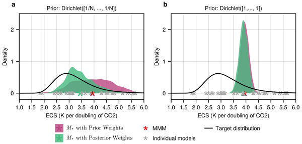
Figure 8 Distributions of expected ECS values of weighted ensembles with N=38 CMIP6 models, based on prior (pink) and posterior (green) weights, using a Dirichlet prior distribution with (a) $\mathit{\alpha }=\frac{\mathrm{1}}{N}$ and with (b) α=1. The black curve is the likelihood function and represents the estimated range of ECS values from Sherwood et al. (2020).

Figure 9 Projected increase in global mean near-surface air temperature with respect to the time period from 1995–2014 until the end of the century, under emission scenario SSP5-8.5, using an ensemble of N=38 CMIP6 models. Thick lines show the observations (black), the multi-model mean (orange) and the weighted averages, using the mean posterior (blue) and mean prior (dashed purple) weights when applying the ensemble performance weighting approach with prior Dirichlet ($\frac{\mathrm{1}}{N}$) and with the target distribution from Fig. 8 as likelihood. Uncertainty bands (shaded regions) represent the 0.05 and 0.95 quantiles of the predicted (weighted) ensemble spread.

We aim to infer the posterior probability of weight vectors w given model output M (here referring to the models' ECS values):

$$\begin{array}{}\text{(14)}& P(\mathit{w}\mid M)\propto P(M^{*}\mid \mathit{w})\cdot P\left(\mathit{w}\right).\end{array}$$

We use all CMIP6 models for which we have ECS values, as well as near-surface-air temperatures for the historical time period from 1850–1900 and under the shared socioeconomic pathway scenario 5-8.5 (SSP5-8.5) available (N=38). As likelihood function, i.e. to evaluate the “performance” of a weighted average model, that we also refer to as ℳ_* model, we use the distribution of likely ECS values that Sherwood et al. (2020) derived based on various lines of evidence. For the prior distribution over weight vectors w we use a Dirichlet distribution. As we showed in Section 3, the choice of the parameterization of the Dirichlet prior distribution is important since it influences the range of the considered data (here ECS values) of the resulting ℳ_* models. Ideally, we want the prior weights to span the entire range between 0 and 1 so that a large part of the individual models' ECS values is covered by the prior weighted average models. We achieve this by setting the concentration parameter α to $\frac{\mathrm{1}}{N}$. Figure 8 shows the distribution of the ECS values for the weighted average models (ℳ_*), based on the prior (pink density) and posterior weights (green density), using Dirichlet$\left(\mathit{\alpha }=\frac{\mathrm{1}}{N}\right)$ (left) and, for comparison, using Dirichlet(α=1) (right). Only when the prior is sufficiently broad (Fig. 8a), does the mean ECS value of the ℳ_* models, computed based on the posterior weights, shift towards the likely range of the target distribution at around 3 °C, below the multi-model mean. When α=1 (Fig. 8b), the range of a priori considered ECS values tightly sits around the multi-model mean as, with this parameterization, on average each model receives equal weight.

We use the computed posterior over weight vectors and apply it to future projections of the increase in global mean near-surface air temperature. As shown in Fig. 9, the expected increase in global mean temperatures is lower in the weighted (blue) than in the unweighted (orange) ensemble which we would hope to see, given the known tendency of CMIP6 models to overestimate future warming (e.g.  Tokarska et al., 2020; Hausfather et al., 2022). The uncertainty range (inner 90 % quantile) is substantially reduced in the weighted ensemble (posterior weights, blue shaded region) as compared to the unweighted ensemble spread (orange shaded region). A reduced uncertainty range is expected by the mere fact that we consider weighted averages. For comparison, the purple shaded region in Fig. 9, shows the 0.05 and 0.95 quantiles for the prior weighted ensemble, i.e. using the prior weights (Dirichlet$\left(\mathit{\alpha }=\frac{\mathrm{1}}{N}\right)$). The 90 % inner quantile range of the unweighted ensemble is in between 1.26 and 1.56 times larger than the 90 % inner quantile range of the prior weighted ensemble (mean 1.36). This shows how much of the reduced uncertainty of the posterior weighted ensemble is just due to the choice of the prior distribution, and how much can be attributed to the data. In any case, it is important to note that the weighting is not necessarily better the smaller the resulting uncertainty range is. If, in the ensemble weighting approach, the prior strongly restricts the considered weighted averages (as in Fig. 8b), this will influence the uncertainty range of the weighted ensemble for the target variable in that it will be unreasonably small. Therefore, in the ensemble performance weighting approach, prior predictive checks become indispensable for a reasonable interpretation of the weighted ensemble. Figure A1 in the appendix (Sect. A) shows the drastically reduced uncertainty range for the weighted projections when using a Dirichlet prior with α=1, i.e. corresponding to the data in Fig. 8b.

How skillful a weighting approach generally is compared to using an unweighted ensemble should furthermore always be assessed through tests (Abramowitz et al., 2019). If the computed weights are based on historical data, perfect model tests are an option, where one model is removed from the ensemble, and its output is considered as “observations”. It can then be checked whether the pseudo-observations lie in the predicted range for future timesteps. This procedure is then repeatedly done, each time using a different model as “perfect model” (e.g., see Brunner et al., 2020). Another option is classical calibration-validation where a subset of the observed data is left out for computing the weights. These data can then be used to test whether the weighted ensemble predicts the out-of-sample data better than the unweighted ensemble. Using ECS as a basis for assessing model performance, as we do here, is different in that it involves an independently derived likelihood function. In this case, one option is to check whether the ECS-based weighting is valuable for weighting the model output for the historical period. As expected due to the relatively small influence of ECS on the warming in the historical period and after consideration of the results in Fig. 9, the ECS-based weighting is not particularly valuable to weigh the historical period. The summed RMSEs between the observations and the predicted mean values across all years between 1950 and 2014, is nearly identical for the unweighted and the weighted M_* model using the mean posterior weight vector. With the weighted ensemble, the RMSE is only marginally smaller (37.68 vs. 37.83 or on average per timestep 0.5796 vs. 0.5820). However, long-term warming is much more strongly governed by ECS than near-term warming, so that the influence of ECS-based weights, in terms of the divergence between weighted and unweighted projections, is larger for projected future warming.

7 Discussion

With this paper we aimed to find a common language to categorise different ways to compute model weights, describe the different choices that have to be made together with their implications, and generally highlight their advantages and disadvantages. Despite the focus of the paper on an application in the climate domain, the discussed approaches may be relevant for ensemble weighting problems across domains as the problems faced by combining any ensemble of individual models are generally similar (e.g., see Riccio et al., 2007; Potempski and Galmarini, 2009; Solazzo et al., 2013). We differentiate between two general approaches: ensemble and individual performance weighting. While in the former weights are computed based on the performance of a linear combination of all models, in the latter, weights are computed directly from the performance of each individual model.

As we showed by means of toy examples, a practical advantage of the ensemble performance weighting approach is that it implicitly accounts for the issue of inter-model dependencies since each weight represents the relative contribution of the corresponding model to the weighted average instead of representing its performance as such. Put differently, the mean weight from the ensemble performance approach depends not only on how closely the model simulates the observed data, but also on the other models in the ensemble: If there is a model m_j in the ensemble that provides the same information as a model m_i, the average weight for both models will be reduced accordingly. Similar to defining model independence in terms of model output similarities, the “independence” part in the resulting mean weight vector, obtained from applying the ensemble performance weighting approach, does not directly depend on the observational data. While some consider it an advantage of the independence weights to not depend on observational data (e.g. Brunner et al., 2020), others argue that the distance to observational data should have an influence on the independence weights (e.g. Abramowitz et al., 2019). In any case, what can be noted is that neither the individual performance weighting nor the ensemble performance weighting approach takes into account whether two models represent the relevant physical processes for the target output variable in the same way or differently. Even if two models have similar output, they perhaps still should be considered independent (i.e. not be downweighted) if their outputs result from different representations of the underlying processes. Similarly, two models that generate different outputs, but share similar representations, should be considered less independent (i.e. be downweighted) than they are based on their different outputs. Note that in terms of the influence on the uncertainties, the worst case yet is when models with similar outputs are not downweighted and the similar outputs result from similar representations of the underlying process as in this case, the result would be an underestimation of the uncertainties.

We further considered two additional aspects under the ensemble performance weighting approach, namely the use of multiple diagnostics to measure performance as well as the influence of the choice of the prior distribution over weights. When using multiple diagnostics, we showed that applying them jointly so that the weights are tuned to maximize the overall likelihood, i.e. encompassing all diagnostics, yields better results in terms of the summed RMSE between the weighted average model (using the mean posterior weight vector) and the observed data than applying the diagnostics sequentially and then taking the average of the computed weight vectors. The choice of which diagnostics are most appropriate for measuring performance is a big question on its own (e.g., see Gleckler et al., 2008) that we have not addressed here. Since, in the case of climate projections, we are assessing the performance of physical models, it makes sense to analyze variables that are related to the basic dynamic processes relevant for the target (Katzenberger et al., 2026). In any case, it should always be made clear that there is no universal answer and that any probabilistic projections are conditional on the metrics and diagnostic climate variables that were used. Furthermore, when multiple diagnostics are considered, these should be as independent of one another as possible since otherwise we would run into the same problem that we have with co-dependent models in the individual performance weighting approach: good models (diagnostics) would be erroneously overestimated while poor models (diagnostics) would be erroneously underestimated.

Our example of using ECS as a performance metric demonstrates the importance, in the ensemble performance weighting approach, of choosing an appropriate prior distribution for the weight vectors. For any set of weight vectors, the resulting set of the weighted averages (of the diagnostic variable) will have a reduced spread as compared to the unweighted ensemble. How much it is reduced, however, strongly depends on the nature of the set of applied weight vectors. Both, Dirichlet(1) and Dirichlet($\mathrm{1}/N$), are natural choices for the prior distribution as in both cases the expected value of the weight for each model equals $\mathrm{1}/N$. With Dirichlet($\mathrm{1}/N$) large model weights are similarly likely as smaller model weights whereas with Dirichlet(1), on average, the individual model weights tend to be smaller. Therefore, the Dirichlet(1) prior is much more constrained towards values that lie near the expected value than is the Dirichlet($\mathrm{1}/N$) prior. This, in turn, means that much more data would be necessary, using Dirichlet(1), to end up with a posterior distribution that assigns most probability mass on values in the tails of the distribution. Thus, we generally recommend to use a Dirichlet prior with shape parameter $\mathrm{1}/N$ and to further make prior predictive checks that ensure that the data that is a priori generated by the weighted average models is realistic and largely covers the range of data from the ensemble members. Moreover, for a reasonable interpretation of the projected likely range of the weighted ensemble, using the expected weight of the posterior distribution obtained from applying the ensemble performance weighting approach, it is necessary to verify how much of the reduced range is effectively attributable to the data and not a mere effect of the averaging itself. Therefore, a comparison between the weighted projections based on the prior weights and based on the posterior weights is a minimal requirement to validate the weighting (see Fig. 9).

In fact, the interpretation of the projected uncertainty range, and the interpretation of the uncertainties in general, deserve some further discussion. The predicted uncertainty range for our target variable (e.g., future projections of the increase of global mean temperature in Fig. 9) based on the computed posterior weight vectors in part represents the uncertainty in the computed weights themselves. This is a kind of uncertainty that cannot be included by its nature in the individual performance weighting approach. However, accounting for it does not automatically imply that structural differences between the models are well treated. For large ensembles, this is likely not so problematic, as the ensemble members can be expected to be diverse enough to represent all plausible model trajectories. However, care should be taken when ensembles of opportunity are used, to ensure the uncertainty estimate is not overly narrow. In addition, to get a more representative estimate of the uncertainty around future projections, it would be important to include other kinds of uncertainties that we have not considered here and are often ignored. This includes the uncertainty of the individual models themselves (which can be estimated based on multiple model runs) as well as the uncertainty of the observations that are used for the performance evaluation. The Bayesian formulation of weighting that we proposed here conveniently allows us to make such additions.

Other ensemble weighting methods exist that may inherently characterize the uncertainty of the ensemble better. For example, mixture-density approaches may offer an alternative that preserves cross-model variance. The adaptation of the classical Bayesian model averaging (BMA) approach from Raftery et al. (2005), for instance, computes mixture densities that combine the probability densities of the individual models (that need to be defined, e.g. via multiple model runs if available), yielding larger uncertainty ranges. They applied this approach to weather forecasts where there is abundant training data and the focus is on short timescales. The need to define a probability density for individual models might be relaxed if a scoring rule comparing cumulative distributions (e.g. Gneiting and Raftery, 2007) is used instead of a likelihood, borrowing from the generalized-Bayes idea (Bissiri et al., 2016). A thorough comparison of these and related approaches like Bayesian stacking (see Yao et al., 2018) is beyond the scope of this paper, but represents a valuable direction for future work.

A limitation of the ensemble performance weighting approach is that it is restricted to linear combinations of individual models. However, in some cases it might be more appropriate to combine models in a non-linear way. Some models, for instance, perform much better in particular regions of the globe than in others, suggesting that the weights may be modeled to differ across grid points, or regions (e.g., Das Bhowmik and Sankarasubramanian, 2021; Thao et al., 2022). As the choice of the diagnostics, whether or not it is helpful to compute weights dependent on a region or even on a grid-point level also depends on the objective. If the objective is to compute the likely range of global mean temperatures in the future, it seems more plausible to stick with one weight per model whereas weights on the level of grid cells may be useful when considering likely ranges of temperatures within a certain region only.

A key focus of this work has been to compare the different assumptions and implications of the individual and the ensemble performance weighting approach. Overall, past work (Massoud et al., 2019, 2020) indicate that ensemble performance weighting provides benefits over individual performance weighting. As just mentioned, there may be cases in which ensemble performance weighting is not appropriate. However, there are many cases in the literature where the final goal is to obtain good performance of the combined ensemble, i.e. we are interested in knowing the weighted-mean prediction. In those cases, ensemble performance weighting is more straightforwardly connected to the goal and provides an estimate of the uncertainty in the weights which is not accounted for in the individual performance weighting approach. If, on the other hand, the goal is simply to rank models or model versions against each other, then the individual performance weighting approach is straightforward in its application.

8 Conclusions

With this paper we aimed to find a common terminology to categorise different approaches to compute model weights that facilitates a comparison between them, and makes their underlying assumptions transparent. For that we distinguish between two general methods that we call the individual performance weighting and the ensemble performance weighting approach. The former comprises all methods that compute a single weight vector where each model is assigned a probability relative to its individual performance while methods belonging to the latter compute a distribution over weight vectors tuned to optimize the performance of the weighted ensemble as a whole. The ensemble performance weighting approach, for instance, has the advantage to implicitly account for model inter-dependencies. However, which method is more appropriate will be different from case to case depending on the target application of the model weights. Here we applied the ensemble performance weighting approach to an ensemble of climate models, but the approach is not constrained to the domain of the Earth Sciences. We have shown that if the ensemble performance weighting approach is applied to compute weighted projections of global mean temperatures, there are two minimal requirements which should ideally both be reported besides the resulting weighted posterior projections: the weighted prior projections, i.e. the projections based on the prior weights, and prior predictive checks that show that the a priori considered weighted diagnostic data reasonably represents the ensemble and does not constrain it too much. Overall, our analyses showed the importance of explicitly acknowledging the influence of our choices, starting with the general approach to compute model weights.

Appendix A: Influence of prior on weighted projections

Figure A1 shows the influence of using a prior distribution over weight vectors in the ensemble performance weighting approach that strongly restricts the considered data. Here, we use a Dirichlet prior with concentration parameter α=1 that yields weight vectors with roughly equal weights assigned to every model. This strongly restricts the output of the weighted average models that are considered a priori as shown in Fig. 8b in the main text. This, in turn, is reflected in Fig. A1 where the shown inner 90 % uncertainty range for the projected increase in global mean temperature is nearly identical when using the prior weight vectors as compared to using the posterior weight vectors. Therefore, this extremely narrow range is not due to the data: we get almost the same uncertainty range simply by using the chosen prior weights without any consideration of the likelihood function.

Figure A1 Like Fig. 9 in the main text, but when using a Dirichlet prior with α=1.

Appendix B

Here we show examples of different weighting approaches that yield the same ranking order and only differ with respect to the magnitude of the individual weights. Note that for simplicity, we left out the area-weights here that should be applied for spatial data.

1. Assume i.i.d Gaussian errors, i.e. $y\left(s\right)=m_i\left(s\right)+\mathit{ϵ}$ with $\mathit{ϵ}\sim \mathcal{N}(\mathrm{0},{\mathit{\sigma }}^{\mathrm{2}})$ and weights for model i are proportional to the likelihood of the data under model i

   • That is, we assume that each data point (y(s)) comes from a normal distribution with the output of model i (m_i) as mean and with standard deviation σ.

   • The likelihood of the observed data under model i is then given by $P(Y\mid M_i,\mathit{\sigma })=\prod _s\frac{\mathrm{1}}{\sqrt{\mathrm{2}\mathit{\pi }{\mathit{\sigma }}^{\mathrm{2}}}}\exp \left(-\frac{y\left(s\right)-m_i(s{)}^{\mathrm{2}}}{\mathrm{2}{\mathit{\sigma }}^{\mathrm{2}}}\right)$, iterating over all data points, e.g. all spatial locations s.

   • The log likelihood of all observed data is then given by: $-\frac{n}{\mathrm{2}}\log \left(\mathrm{2}\mathit{\pi }{\mathit{\sigma }}^{\mathrm{2}}\right)-\frac{\mathrm{1}}{\mathrm{2}{\mathit{\sigma }}^{\mathrm{2}}}\sum _{i=\mathrm{1}}^n{\left(y\left(s\right)-m_i\left(s\right)\right)}^{\mathrm{2}}$

   • turned into a likelihood again:

     $$\begin{array}{ll}{\displaystyle }{w}_i\propto \exp \left(c_{\mathrm{1}}\right)& {\displaystyle }-\exp \left({\displaystyle \frac{\mathrm{1}}{\mathrm{2}{\mathit{\sigma }}^{\mathrm{2}}}}\cdot \sum _{i=\mathrm{1}}^n{\left(y\left(s\right)-m_i\left(s\right)\right)}^{\mathrm{2}}\right.\\ {\displaystyle }& {\displaystyle }\left.=\exp \left(c_{\mathrm{1}}\right)-\exp (c_{\mathrm{2}}\cdot \mathrm{SSE})\right);\end{array}$$

     i.e. $w_i\propto \exp (-c_{\mathrm{2}}\cdot \mathrm{SSE})$ where SSE is the sum of squared errors and c₁, c₂ are constants.

2. Sierra and Muñoz (2025): $w_i\propto \frac{\mathrm{1}}{{\widehat{\mathit{\sigma }}}^{\mathrm{2}}}$ with ${\widehat{\mathit{\sigma }}}^{\mathrm{2}}=\frac{\sum _s\left(m_i\right(s)-y(s){)}^{\mathrm{2}}}{n}=\frac{\mathrm{SSE}}{n}=\mathrm{MSE}$. Therefore, $w_i\propto n\cdot \frac{\mathrm{1}}{\mathrm{SSE}}=\frac{\mathrm{1}}{\mathrm{MSE}}$ with MSE referring to the mean squared error.

3. Brunner et al. (2020) performance weights for a single diagnostic variable: $w_i\propto \exp \left(-{\left(\frac{\sqrt{\mathrm{MSE}}}{{\mathit{\sigma }}_D}\right)}^{\mathrm{2}}\right)$ where σ_D is a tuned hyperparameter.

Appendix C: Short background on statistical concepts used in the paper

For detailed information on all aspects of Bayesian data analysis, you may refer to the classic textbook from Gelman et al. (2013) that is publicly available online (https://stat.columbia.edu/~gelman/book/, last access: 20 October 2026). Here, we briefly summarize the most important concepts used in the paper. In the following, H is a random variable; a specific hypothesis h may for instance refer to the hypothesis that model ℳ_i is “true”. D is the observed data.

Prior

P(H=h) The modeler's prior belief about hypothesis h being true, e.g. P(ℳ_i): probability of model ℳ_i being true, before observing any data.

Likelihood

$P(D\mid H=h)$ The probability of observing data D assuming hypothesis h holds, e.g. the probability of observing data D assuming that it was generated under hypothesis h, for instance by model ℳ_i.

Posterior

$P(H=h\mid D)$ The modeler's posterior belief about a hypothesis h, i.e. after having seen data D, e.g. P(ℳ_i∣D).

Baye's rule

Belief update based on new evidence D.

$$\begin{array}{}\text{(C1)}& P(H=h\mid D)={\displaystyle \frac{P(D\mid H=h)\cdot P(H=h)}{P\left(D\right)}}\end{array}$$

MCMC

Markov Chain Monte Carlo. A class of algorithms that is used to draw samples from probability distributions which are too complex to be solved analytically.

Dirichlet distribution

Dir(α). Continuous probability distribution parameterized by a vector α of length K. Samples from Dir(α) are vectors x of length K where $x_i\in [\mathrm{0},\mathrm{1}]$ and $\sum _{i=\mathrm{1}}^K{x}_i=\mathrm{1}$. When α_i is identical for all $i\in \mathrm{1},\mathrm{\dots }K$, the parameter α can be replaced by the single scalar α, the concentration parameter. For illustration, Fig. C1 shows the distribution of the first element (w₁) in 1000 vectors of length 3 (representing an ensemble of 3 models) sampled from different Dirichlet distributions parameterized with concentration parameter α (the distributions for w₁, w₂ are similar). While for $\mathit{\alpha }=\frac{\mathrm{1}}{\mathrm{3}}$ (middle), values in the middle of the range are sampled, for $\mathit{\alpha }=\frac{\mathrm{1}}{\mathrm{30}}$, these become very few. Figure C2 shows the maximal weight in each vector of length 38, sampled from Dirichlet$\left(\mathit{\alpha }=\frac{\mathrm{1}}{\mathrm{38}}\right)$ (left) and sampled from Dirichlet$\left(\mathit{\alpha }=\frac{\mathrm{1}}{\mathrm{380}}\right)$ (right). While for $\mathit{\alpha }=\frac{\mathrm{1}}{\mathrm{38}}$, the maximal weights are spread across the entire range of values, for $\mathit{\alpha }=\frac{\mathrm{1}}{\mathrm{380}}$ the maximal weight tends to be very high, i.e. the sampled vectors are close to one-hot vectors, assigning nearly all weight to a single model.

Figure C1 Histograms of the first element (w₁) in 1000 vectors (of length 3) sampled from a Dirichlet distribution parameterized with different values of the concentration parameter α.

Figure C2 Histograms of the maximum element in each of 1000 vectors sampled from a Dirichlet distribution parameterized with $\mathit{\alpha }=\frac{\mathrm{1}}{\mathrm{38}}$ (left) and $\mathit{\alpha }=\frac{\mathrm{1}}{\mathrm{380}}$ (right).