Unexpected land-surface warming following a relatively limited-forcing hypothetical nuclear war

Nuclear conflicts could ignite intense fires that inject considerable amounts of black carbon (BC) into the upper troposphere and lower stratosphere, with the potential to disrupt global climate. While uncertainties in the BC injection remain large, relatively few modeling studies have explored the climatic response to more limited nuclear exchange between major nuclear powers. Here, we investigate the climate response to a set of relatively limited-forcing scenarios (12 to 24 Tg BC) for nuclear exchanges between the United States and Russia. This corresponds to one-tenth to one-fifth of the forcing strength of typically considered. We use the Canadian Earth System Model version 5, an independent contributor to the worldwide set of Earth System Models that has not been explored previously in this application. Consistent with previous work, decreased downwelling shortwave radiation at the surface drives prolonged surface cooling. Unexpectedly, however, a transient surface warming develops in the first boreal summer following a boreal-winter injection, linked to reduced cooling via net longwave and turbulent fluxes. The transient warming is most pronounced for the lowest forcing cases. Precipitation, which decreases even while the surface warms, is found to be controlled by stabilizing, top-heavy warming. Multi-model assessment of these relatively limited-forcing cases is warranted given their potential impacts.

1 Introduction

Although the global nuclear arsenal has shrunk since the Cold War, global society is still threatened by potential nuclear conflict due to rising geopolitical tension and the proliferation of regional nuclear powers. In addition to local damage and health effects at the locations of nuclear detonation (Lucas et al., 1990; Solomon and Marston, 1986), regional nuclear conflicts can have global climatic effects, including stratospheric warming, surface cooling, and reduced precipitation (Coupe et al., 2019; Robock et al., 2007a; Toon et al., 2007, 2019) as well as reduction in the ozone layer thickness (Bardeen et al., 2021; Mills et al., 2008, 2014, Yook et al., 2025).

The global effects stem from firestorms that are triggered at targeted urban and industrial centers. The firestorms can induce convection capable of injecting a great amount of inorganic and organic carbon into the upper troposphere – lower stratosphere (UTLS) (Tarshish and Romps, 2022; Toon et al., 2007). Climate modeling studies have shown that the carbonaceous aerosol can heat the upper atmosphere and cool the Earth's surface by increasing the absorption of solar radiation aloft (Pausata et al., 2016; Robock et al., 2007a). Upon local heating, the aerosol-laden air becomes buoyant and rises to a higher altitude. This “self-lofting” prolongs the aerosol residence time (Johnson and Haywood, 2023; Malone et al., 1985; Ohneiser et al., 2023). In a hypothetical case of a full-scale nuclear exchange between the United States and Russia, a UTLS injection of a large amount of black carbon (BC) would drive unprecedented stratospheric warming and surface cooling at a global scale (Robock et al., 2007a). The surface cooling may lead to crop failure and famine, slowing down societal recovery (Xia and Robock, 2013; Xia et al., 2015, 2022). Precipitation would also be reduced globally due to reduction in solar heating, evaporation, and convection. Disruption of stratospheric chemistry would lead to ozone depletion via various mechanisms even for a modest BC injection in a nuclear conflict between India and Pakistan (Mills et al., 2008, 2014). The resulting increase in surface UV radiation could damage human health and ecosystems on a global scale.

Both the amounts of BC emission and UTLS injection are highly uncertain. Taking into account the uncertainties in the BC-emission factors of flammable materials and the quantities to be burned, Turco et al. (1990) considered a wide range of plausible BC emissions, from 20 to 290 Tg, that could arise as a result of a full-scale nuclear exchange involving the North Atlantic Treaty Organization (NATO) and Warsaw Pact nations. Beside emission factor uncertainty, variations in local meteorology, modern warfare tactics, and rubblization of fuels all contribute to the uncertainty in the total amount of BC injected into UTLS (Glasstone and Dolan, 1977; NASEM, 2025; Tarshish and Romps, 2022). However, for this full-scale nuclear exchange scenario, most studies considered a UTLS injection of 150 Tg BC (Bardeen et al., 2021; Coupe et al., 2019; Robock et al., 2007a), with little attention given to relatively limited-forcings involving smaller BC injections from more limited exchanges between major nuclear powers. Yet a nuclear conflict would not necessarily entail the use of the entire arsenal; assessing the climate effects of such partial or regional exchanges is therefore essential to capture the plausible range of outcomes. In this context, smaller injection estimates on the order of 10–25 Tg BC become particularly relevant, as they represent plausible outcomes of limited nuclear exchanges rather than full-scale global war. BC injections of this order of magnitude have been considered for the India-Pakistan exchange scenario, for example by Toon et al. (2019), but the climate effects are expected to be different for major nuclear powers, such as for the USA-Russia scenario. In this case, the injection latitudes are farther away from the rising branch of the Brewer-Dobson circulation (Butchart, 2014). A UTLS injection of 10–25 Tg BC for the USA-Russia scenario would be relatively small compared to the 150 Tg load in Coupe et al. (2019) and Robock et al. (2007a) but still extreme relative to natural forcing or recent forest fires. For comparison, the 2019 Australian wildfires emitted 0.9 Tg of smoke into the stratosphere, of which 2.5 % was BC, and the remainder was mostly organic carbon (OC) (Yu et al., 2021). Model calculations estimated a statistically significant warming and ozone depletion in the southern hemispheric midlatitude stratosphere for 6 months as a result of these wildfire emissions. Compared to typical wildfires, the smoke injected into the UTLS would have a higher BC-to-OC ratio due to lower oxygen content in large-scale urban fires (Shemwell and Levendis, 2000; Tewarson, 2002; Toon et al., 2007). Therefore, it is a pertinent question to ask how the climate response might differ under a relatively limited BC injection scenario in the extratropics.

In this study, we look into the climate response to such a relatively limited BC injection with the use of an atmosphere-ocean coupled model, the Canadian Earth System Model version 5.1 (CanESM5; Swart et al., 2019). This is the first time CanESM is used for the study of nuclear war fire emissions. Its independent development from other climate models helps characterize model uncertainty. Although it is a low top model with a coarse stratospheric representation and a lack of stratospheric chemistry and aerosol model, it is a workhorse ESM that has been extensively used in many climate simulations studying anthropogenic climate change effects stemming from the Coupled Model Intercomparison Project phase 6 (CMIP6; Eyring et al., 2016; Samset et al., 2025). We test the sensitivity of the response by varying the total BC injection around the low end of the estimated emission in a full-scale nuclear exchange, between 12 and 24 Tg. This study represents an effort to investigate this model's climate response to such forcing before the CanESM system moves to subsequent more advanced versions with updates to the aerosol scheme. In this study, we find a previously undocumented transient “whiplash” as the model transitions to a nuclear winter state through an early summertime warming response, unexpectedly strong high-latitude responses to stratospheric BC injection, and other effects. This relatively limited but plausible forcing scenario bears investigating in other models.

In Sect. 2, we provide a description of the model used and parameterizations of relevant processes, as well as the experimental set-up. In Sect. 3, we investigate the climate response to different amounts of BC emission in the relatively limited-forcing scenarios. In Sect. 4, we summarize the results and discuss the potential implications and future work.

2 Methods

2.1 Model description

We conduct the simulations using the Canadian Earth System Model version 5.1 (CanESM5; Swart et al., 2019), which contains an atmosphere component that incorporates a land model, coupled with the ocean model NEMO (Madec and the NEMO team, 2013). The atmosphere component of CanESM5 is the Canadian Atmospheric Model version 5 (CanAM5) with a bulk aerosol scheme employed (Cole et al., 2023). It is a T63 spectral dynamical core model (2.8° horizontal resolution) with 49 vertical layers with layer thickness that increases monotonically from approximately 100 m at the surface to 2 km at about 1 hPa, which is the upper bound. The number of vertical levels has been increased from its predecessor, CanAM4 (von Salzen et al., 2013), to match those employed by the Canadian Middle Atmosphere Model (Scinocca et al., 2008), but the stratosphere is still coarsely represented, with 18 levels from about 300 to 10 hPa. The quasi-biennial oscillation is not simulated by CanAM5. Biases in stratospheric temperature and zonal wind are reduced in CanAM5 relative to CanAM4 (Cole et al., 2023). Despite having a low model top, CanESM5 has been used in the framework of understanding climate perturbations involving dynamical and radiative coupling of the troposphere to the lower stratosphere. For example, it has been used in the Model Intercomparison Project on the climatic response to volcanic forcing (VolMIP; Zanchettin et al., 2016), which is an endorsed contribution to the CMIP6. It also has good performance in realizing the Arctic sea-level pressure response to sudden stratospheric warming among CMIP6 models when compared to reanalysis (Dai et al., 2024), suggesting that it simulates stratosphere-troposphere interactions adequately for our sensitivity study.

CanAM5 employs bulk cloud microphysical parameterizations that depend on the mean water content and other moments of droplet size distributions (von Salzen et al., 2013). The autoconversion, cloud liquid water content, and cloud lifetime depend on a cloud droplet number concentration that is a function of sulphate concentration (Ghan et al., 2013; Wood, 2005). The latter parameterization represents what is known as the second aerosol indirect effect. CanAM5 also parameterizes the BC semi-direct radiative effect as a perturbation to existing liquid cloud optical properties according to the volume fraction of BC to cloud water (Li et al., 2013). The cloud processes are limited to pressures greater than 10 hPa given the uncertainty in the applicability of the parameterizations at high altitudes. Aerosols that are considered in CanAM5 include sulfate, BC, OC, sea salt, and mineral dust. Hydrophilic BC, hydrophilic OC, and sulfate are assumed to be internally mixed in CanAM5 and have a refractive index that depends on the fraction, effective radius, and effective variance of each component aerosol, as well as the relative humidity (Wu et al., 2018). The assumed hydrophilic BC effective radius and variance are 0.166 µm and 0.617, respectively. CanAM5 does not take into account the aerosol number for determining gravitational settling rate, unlike some other models that have been used for the climate impact study of nuclear conflicts such as NorESM1-M (Pausata et al., 2016) and CESM2-WACCM6 (Gettelman et al., 2019).

Aerosols are removed from the atmosphere by dry and wet deposition. In CanAM5, the dry deposition flux is parameterized based on near-surface aerosol concentration and a specified dry deposition velocity that depends on the type of tracer and the local surface condition (Croft et al., 2005; Lohmann et al., 1999). For wet deposition, CanAM5 includes below-cloud scavenging for stratiform clouds and in-cloud scavenging for both stratiform and convective clouds. The below-cloud scavenging rate depends on the precipitation rate, whereas the in-cloud scavenging rates depend on the precipitation formation rate. The snow-darkening effect of BC deposition is also included in CanAM5. The total BC deposition flux is used to calculate the BC mass budget in snow layer, whose snow albedo is parameterized as a function of BC mass mixing ratio in snow, snow water equivalent, snow grain size, underlying surface albedo, and solar zenith angle (Namazi et al., 2015).

2.2 Experimental design

We generate an ensemble with an injection of 20 Tg of BC (hereafter as BC20), consisting of 15 ensemble members. To generate the ensemble members, we select different years from a 100-year pre-industrial control simulation as the initial years (Eyring et al., 2016). All selected years are at a neutral state of the El Niño-Southern Oscillation (ENSO) in January to avoid potential ENSO imprint on the simulated responses. To test the sensitivity of the global mean climate response to BC aerosol, we generate 3 additional ensembles with an injection of 12, 16, and 24 Tg of BC (hereafter as BC12, BC16, and BC24), consisting of 9, 3, and 8 members, respectively. While we were interested in extending beyond this limit, we have found that the model was rendered unstable for forcings greater than about 40 Tg and that the climate response exhibits unexpected features even in the relatively limited-forcing scenarios. All injected BC particles are assumed hydrophilic from the start. As in previous studies, the particles are injected uniformly between 300 to 150 hPa over the United States and Russia at a constant rate over 1 week, starting from 1 January. To evaluate the long-term response, each simulation is run for 20 years from the first day of emission. A response is calculated by subtracting the climatology of the 100-year control simulation from the average of all ensemble members.

3 Results

3.1 BC burden response and impacts on global shortwave and longwave radiation

For all cases, more than two-thirds of the BC burden stays under the overworld, which is defined as the domain above the 380 K potential temperature surface (around 15 km above the Earth's surface) (Holton et al., 1995), and gets removed in the first year (Fig. 1a). The BC burden in the lower atmosphere (under the 380 K potential temperature surface) is relatively greater in the first year before getting removed, which is important for the shorter-term climate response. The overworld burden for BC12 attains its maximum at 2.0 Tg in first year June, while the overworld burden for BC24 attains its maximum at 5.2 Tg in the same month, so doubling the injection from 12 to 24 Tg results in more than 2.5 times more BC being lofted into the overworld. After reaching the maximum burden in the overworld, the overworld BC mass e-folding time, which is defined by the time it takes for the burden to reach e⁻¹ of its maximum, for BC16, BC20, and BC24 is estimated between 3 years and 6 months, and 3 years and 8 months, while the mass e-folding time for BC12 is 3 years and 3 months. In the lower atmosphere, the mass e-folding time is 3 months for all 4 cases. Throughout the simulated period, the fraction of remaining mass of BC is greater in the larger-forcing scenario (Fig. 1b). The nonlinear dependence of early-stage BC lofting on the total mass of injection influences the long-term climate response since the overworld burden has a much longer residence time compared to lower atmospheric burden.

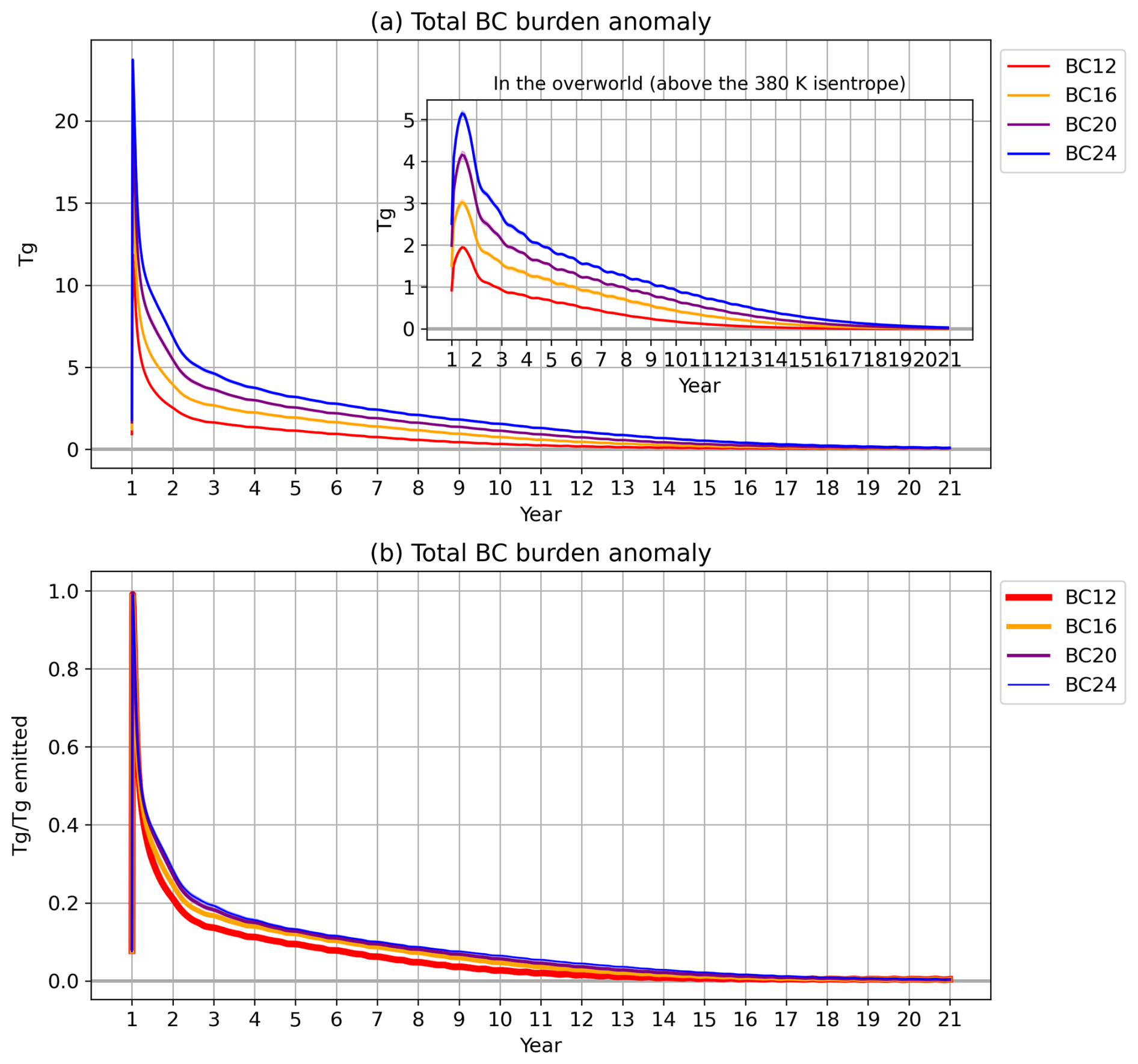
Figure 1 Daily mean BC burden anomalies relative to the control simulation (a) in the atmosphere, (inset of panel a) in the overworld domain, and (b) in the atmosphere per Tg of emitted BC. Shading indicates ±1 standard error of the ensemble mean. In panel (b), the lines for different ensembles are varied in thickness to show where they overlap.

As will be shown, the climate responses exhibit distinct behaviours during January to February (JF) of first year, June to August (JJA) of first year, and years 6 to 15. The temporal means of the climate responses for these primary periods of interest will be highlighted throughout this section (Table 1).

Table 1 Temporal means of the global responses of DSRF (in W m⁻²), DLRF (in W m⁻²), and surface temperature (TS; in °C) for BC24 (BC12 in parentheses), with the 95 % confidence intervals. For first year JF (or first year JJA), the aggregated timeseries used for the confidence interval calculation is the aggregation of first year JF mean (or first year JJA mean) of all ensemble members, so the number of samples is the number of members. For year 6–15, the aggregated timeseries is the aggregation of all monthly output in year 6–15 of all ensemble members. The number of samples is the ensemble mean effective sample size after applying a lag − 1 autocorrelation to the monthly timeseries of each ensemble member, assuming first-order autoaggressive dependence.

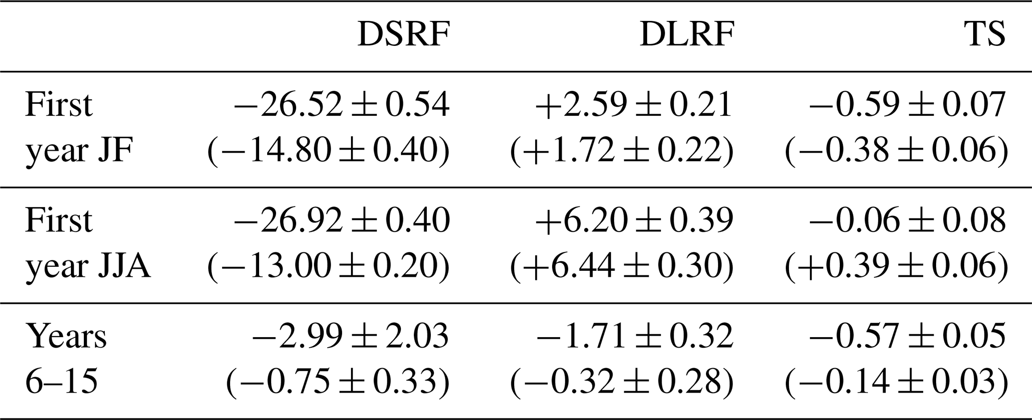
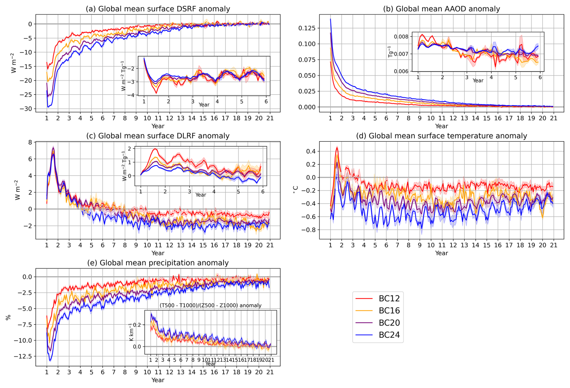
Figure 2 Monthly averaged global mean responses of (a) surface DSRF, (b) AAOD, (c) surface DLRF, (d) surface temperature, and (e) precipitation. Insets of panels (a) and (c) are the radiative flux responses divided by the atmospheric BC burden, respectively. Inset of panel (e) is the monthly averaged global mean responses of the temperature difference between 500 and 1000 hPa, divided by the thickness of the column. Shading indicates ±1 standard error of the ensemble mean. Dashed lines indicate where the standard error overlaps with the zero line.

Absorption of solar radiation by BC reduces surface downwelling shortwave radiative flux (DSRF). The response in the global mean surface DSRF reaches a minimum in two months following the UTLS injection of BC (Fig. 2a). The response is −14.80 and −26.52 W m⁻² in first year January and February for BC12 and BC24, respectively (Table 1). As the BC aerosol is removed from the atmosphere, the response gradually diminishes. The reduction in the global mean DSRF per unit mass of burden has not been maximized in the first two months when the global mean DSRF reduction reaches the maximum since the BC aerosol is still concentrated in the Northern Hemisphere (NH) (Fig. 2a inset and see description of Fig. 3a on BC interhemispheric transport). The efficiency of reduction is maximized in July of the first year as the BC is transported globally (see below). Doubling the BC injection from 12 to 24 Tg causes the reduction per Tg burden to decrease from −3.6 to −2.9 W m⁻² Tg⁻¹ in first year JJA (Table 1). After the first year, the surface DSRF reduction per Tg burden is comparable across all the cases. This indicates approximately a linear scaling of the surface DSRF reduction with the atmospheric burden of BC, which is expected for relatively limited-forcing scenarios. Although the surface DSRF reduction per Tg burden is comparable across the scenarios, the BC burden decreases at a faster rate for the weaker forcing scenarios (Fig. 1b), resulting in a smaller surface DSRF reduction per Tg injection in the long term (Table 1). Comparing BC12 and BC24, the surface DSRF reduction per Tg injection for BC12 is initially comparable to that for BC24 but becomes only about half of the value for BC24 in years 6 to 15 (Table 1). This implies that by allowing more BC aerosol to reach the overworld, the stronger early-stage self-lofting effect in BC24 contributes to the reduction of DSRF at the surface in the long term. This translates to a nonlinear response in the long-term surface temperature response, as will be shown below.

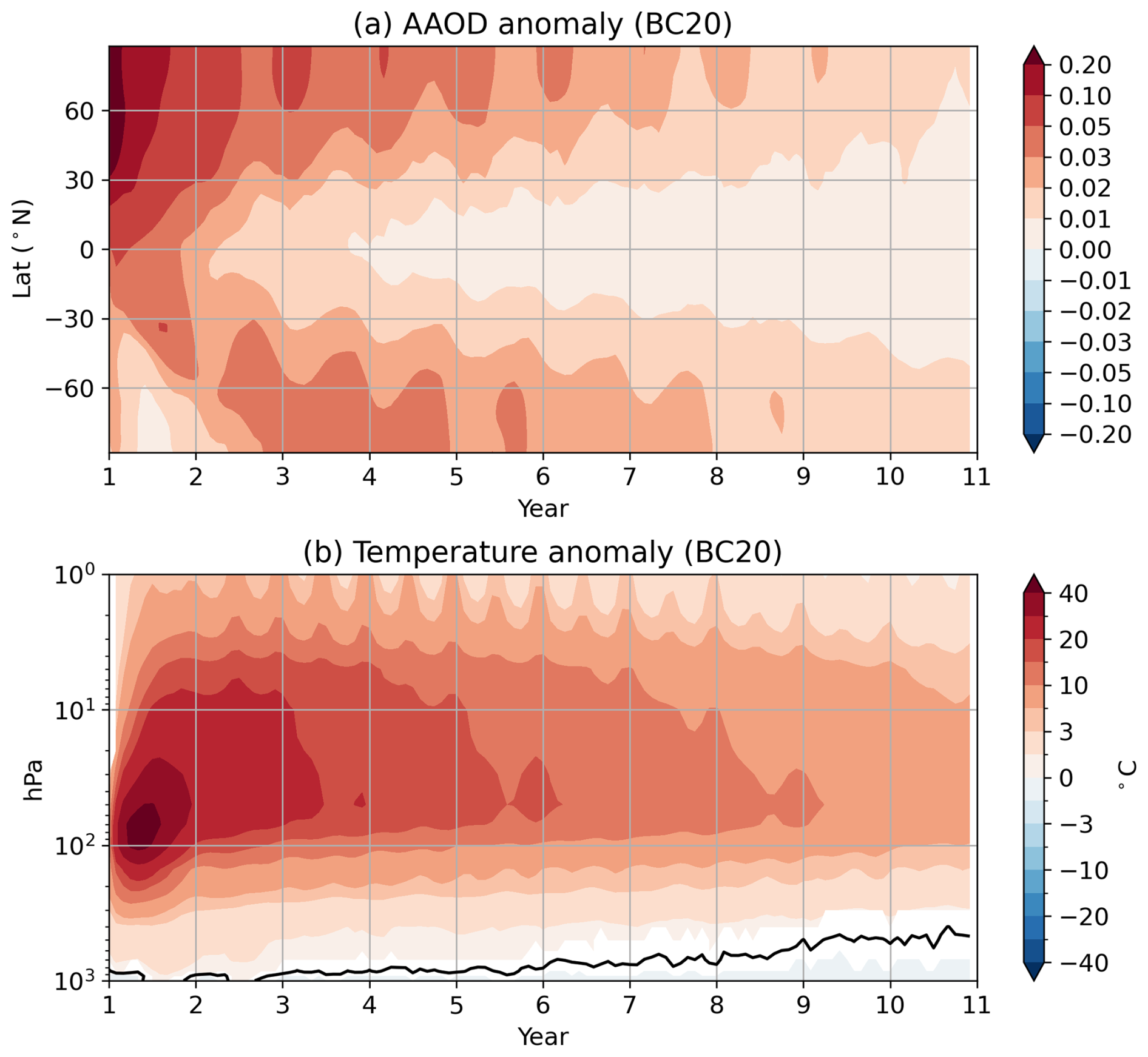
Figure 3 Monthly averaged responses of (a) zonal mean aerosol absorption optical depth at 550 nm and (b) horizontally averaged air temperature. White patches indicate changes that are not significant at the 95 % confidence level using a t test. In panel (b), solid black line is the line of 0 K.

The global mean aerosol absorption optical depth (AAOD) response is consistent with the surface DSRF response (Fig. 2b), also with an approximately linear scaling (Fig. 2b inset). Unlike the surface DSRF response, the AAOD response starts at its extremum since it depends on the relative radiant flux absorbed by the aerosol rather than the absolute change in the radiative flux. For our best-sampled simulation, BC20, the zonal mean AAOD ranges from 0.1 to 0.3 in most of NH in the first simulated year (Fig. 3a). The AAOD becomes comparable between the hemispheres after about 2 simulated years and is reduced to about 0.01–0.02 at high latitudes after 10 years.

In addition to the perturbation to shortwave radiative transfer, the longwave radiative transfer would also be perturbed by the aerosol injection due to changes in emissivity and thermal structure of the atmosphere (Ramaswamy and Kiehl, 1985). The surface downwelling longwave radiative flux (DLRF) response is initially negligible and then increases as the atmosphere is heated by the BC (Figs. 2c, 3b). For the best-sampled scenario, BC20, the global mean air temperature response exceeds 40 °C at 70 hPa in the first April following the injection and attains a maximum of 45 °C at 70 hPa few months later in June at the beginning of the boreal summer (Fig. 3b). The changes in longwave radiative transfer result in a global mean surface DLRF increase that peaks at +7.33 W m⁻² in August of the first year (Fig. 2c). The response in surface DLRF in first year JJA is similar among the different scenarios (Fig. 2c, Table 1). This implies that the surface DLRS increase per Tg burden in first year JJA is greater for the weaker forcing scenarios than the stronger forcing scenarios, in contrast to the approximate linearity of surface DSRF response (Fig. 2a, c insets, Table 1). In the long term, the positive response of surface DLRF decays faster than the negative response of surface DSRF (Fig. 2a, c).

3.2 Impacts on global temperature and precipitation

The global mean surface temperature is decreased in response to the reduction in surface DSRF, but an unexpected oscillation is seen in the temperature response during the first boreal summer. The reduction in surface DSRF of −14.80 and −26.52 W m⁻² causes a rapid global mean surface cooling of −0.38 and −0.59 °C in first year JF for BC12 and BC24, respectively (Fig. 2d, Table 1). Surprisingly, instead of a gradual return to the climatological mean, the global mean surface temperature response increases drastically until it reaches a maximum in first year JJA. It is +0.39 and −0.06 °C for BC12 and BC24, respectively (Table 1). This implies that the global surface temperature response increases by more than 0.7 °C for BC12 from first year JF to JJA, whereas it increases by 0.5 °C for BC24 in the same period. The surface DLRF increase is consistent with the striking transient surface warming. It peaks at +6.44 and +6.20 W m⁻² in first year JJA, the same season in which the surface temperature response is at its highest (Fig. 2c, d, Table 1). After the temperature peak in first year JJA, the global mean surface temperature transitions back to a negative response and remains somewhat steady in years 6 to 15 before slowly returning to the climatological mean towards the end of the simulations (Fig. 2d). This is consistent with the trade-off between surface DSRF and DLRF, with the positive response of surface DLRF decaying faster than the negative response of surface DSRF (Fig. 2a, c). In years 6 to 15, the global mean surface temperature responses are −0.14 and −0.57 °C for BC12 and BC24 (Table 1). The surface temperature responses per Tg injection are −0.012 and −0.024 °C Tg⁻¹. The nonlinear dependence of surface temperature response on the mass of injection is controlled by the nonlinear dependence of surface DSRF reduction on the mass of injection, −0.06 and −0.12 W m⁻² Tg⁻¹ in years 6 to 15. As mentioned above, the stronger early-stage self-lofting effect in the stronger forcing scenarios contributes to the long-term surface DSRF reduction. Thus, the nonlinear self-lofting effect translates to a nonlinear response in the long-term surface temperature response.

Despite having surface temperature increase in the first boreal summer, the global mean precipitation response remains negative from the start to near the end of the simulations (Fig. 2e). While reduced precipitation is an expected part of the weakened hydrological cycle associated with nuclear winter (Robock et al., 2007a), the pronounced reduction of precipitation during the period of warming in the first year is consistent with the increase in static stability (Fig. 2e inset). The troposphere is stabilized as the upper troposphere is heated by the light-absorbing BC. This is clear from the best-sampled simulation, BC20 (Fig. 3b). Although the lower tropospheric response is a warming in the first boreal summer, the mid-tropospheric warming is greater. The greater static stability inhibits convection and reduces precipitation. The strongest vertical gradient of temperature response between 100 and 500 hPa emerges in the first year and is weakened afterward, but the sign of the temperature response gradient persists until the end of the simulated period, indicating a more stable troposphere throughout the simulation.

3.3 Spatial pattern of impacts on surface temperature

The regional pattern of surface temperature is forcing-dependent. Comparing the first year JJA responses between BC12 and BC24 reveals stronger polar cooling and larger sea ice expansion under higher forcing (Fig. 4). Moreover, mid-latitude warming is less intense in the higher forcing scenario. Although enhanced mid-tropospheric heating may increase DLRF, the stronger longwave effect under weaker forcing remains uncertain and is examined further below.

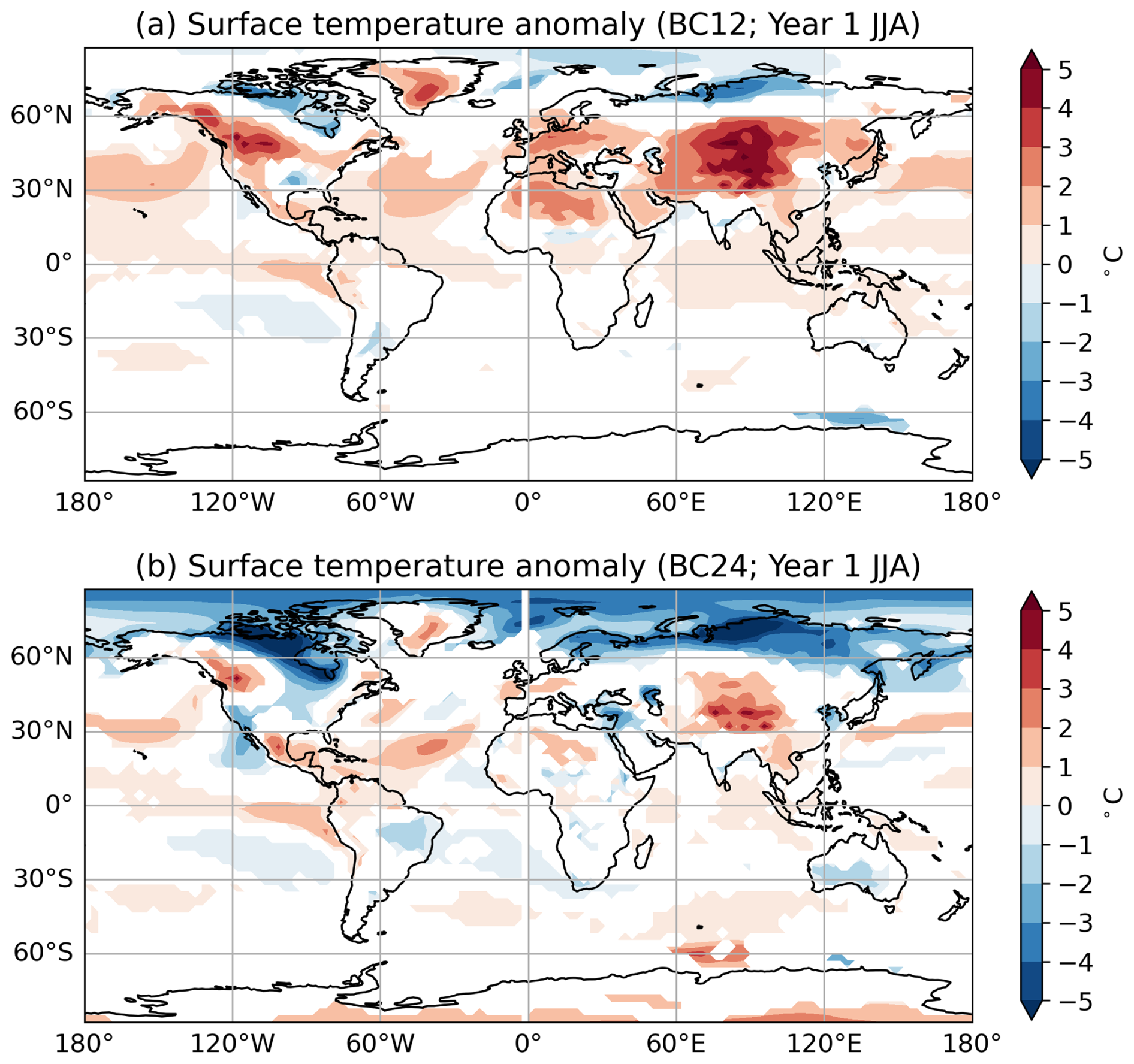
Figure 4 Responses of surface temperature for (a) BC12 and (b) BC24 in JJA of the first simulated year. White patches indicate changes that are not significant at the 95 % confidence level using a t test.

To characterize this transient evolution from the initial year to subsequent years, we show the best sampled simulation, BC20, contrasting JF and JJA of the first year – marked by the pronounced surface temperature oscillation – with the quasi-steady response over years 6 to 15.

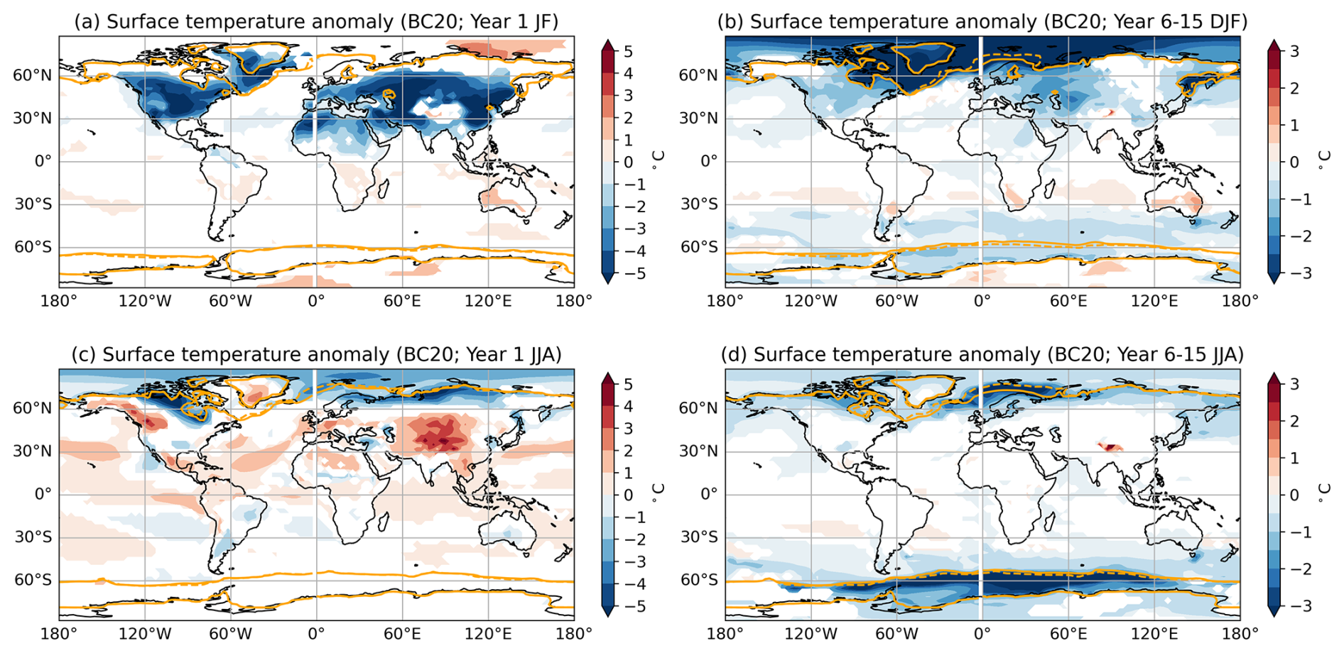
Figure 5 Responses of surface temperature as in Fig. 4 but for BC20 in (a) JF of the first year, (b) DJF of years 6–15, (c) JJA of the first year, and (d) JJA of years 6–15. White patches indicate changes that are not significant at the 95 % confidence level using a t test. The solid and dashed orange lines indicate the sea ice edge for the scenario and for the climatology, respectively. It is defined as the grids with 15 % sea ice area.

In the first two months following the injection, substantial surface cooling is seen on land as a result of the surface DSRF reduction. In NH, there is a statistically significant maximum cooling of about 8 °C in continental regions in the JF-mean (Fig. 5a). The reduction in surface DSRF causes most of the cooling, but the dynamical response likely contributed to some of the temperature responses. For example, the cooling around Greenland and the warming north of Siberia are likely due to a positive Arctic-Oscillation-like (AO) response (Fig. 5a; also see Fig. A1 for the regressed positive AO pattern in the control simulations; Stenchikov et al., 2002). A stronger AO-like response was shown for a 5 Tg India-Pakistan case by Robock et al. (2007b). In December to January (DJF) over years 6 to 15, the maximum cooling is at high latitudes, accompanied by sea-ice extent increase (Fig. 5b). This extends to a significant cooling of 2–3 °C in Europe and around 1.5 °C in southern Canada and the United States.

In the first boreal summer following the fire emissions, substantial warming is seen in parts of Africa, North America, Greenland, and Tibet. A warming of up to +3–5 °C develops around Tibet, +2–3 °C in southern Greenland and the western North America, and +1–2 °C in northern Africa (Fig. 5c; and see Fig. 4 for the corresponding plots for BC12 and BC24). These areas are associated with relatively larger surface DLRF response (Fig. 6a). To deepen our understanding of the longwave effect, we examine changes in cloud, clear sky surface DLRF, and water vapor for the first summer. These warming land regions are clear and arid and experience mixed changes in cloud fraction (Figs. A2, A3), so the longwave effect does not seem to be primarily tied to cloud responses. The global mean clear-sky surface DLRF response is similar to the global mean all-sky surface DLRF response, with the same peak occuring in the first JJA (Figs. A4 and 2c). Both the clear-sky surface DLRF response and the column water vapor response are spatially similar to the increase in all-sky surface DLRF (Figs. A5, A6, and 6a). All three of the responses in water vapor, clear-sky surface DLRF, and all-sky surface DLRF over these land regions that experience warming in the first JJA are greater than those over other land regions, suggesting that downward emission of longwave from BC aloft is being amplified by water vapor feedback for these regions in the first JJA. In these regions, the relative humidity decreases in the UTLS due to intense warming caused by absorption of solar radiation by BC, but it increases in the middle to lower troposphere, which is consistent with water vapor feedback (Fig. 7).

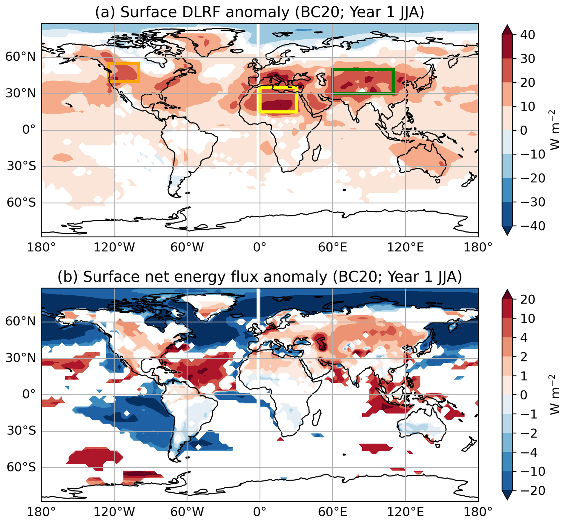
Figure 6 Responses of (a) surface DLRF, and (b) surface net energy flux in JJA of the first year for BC20. The surface net energy flux includes net shortwave radiative flux, net longwave radiative flux, latent heat flux, and sensible heat flux. The fluxes are defined as positive downward. White patches indicate changes that are not significant at the 95 % confidence level using a t test.

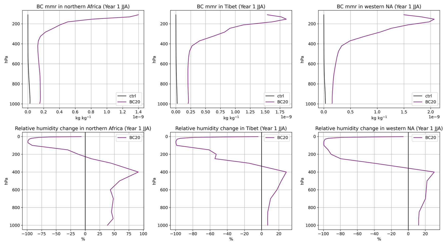
Figure 7 Vertical distributions of the BC mass mixing ratio and relative humidity change over the regions that experience surface warming in the first JJA. The areas of northern Africa, Tibet, and western North America (NA) correspond to the yellow, green, and orange boxes in Fig. 6a, respectively.

To better understand changes in the surface energy exchange, we calculate the full surface net energy imbalance (Fig. 6b), which takes into account net shortwave radiative flux, net longwave radiative flux, sensible heat flux, and latent heat flux (Fig. A7). The surface net energy imbalance is highly localized during the first boreal summer (Fig. 6b). For most land surfaces in NH, the net energy imbalance ranges from +2 to +5 W m⁻² (a positive sign corresponds to warming). Contributing to this positive response is not only an increase in surface net longwave radiative flux (defined positive downward), but also an increase in the turbulent fluxes as the atmospheric stability increases (Fig. A7). Although the net energy imbalance is mostly negative for oceanic surface regions, especially at high latitudes, the higher heat capacity of ocean buffers the ocean surface temperature changes. The localized warming on land with adjustment by advection may result in the temperature response pattern and the positive global mean surface temperature response in the first boreal summer (Figs. 2c, 5c, A8). The long-term response for boreal summer shows statistically significant surface cooling mostly at high latitudes (Fig. 5d).

Overall, these simulations reveal a whipsaw effect on the surface temperature in the first year, where there is a quick transition from the very cold initial conditions to much warmer conditions over midlatitude land surfaces, and then a transition to strong mid-to-high latitude cooling as sea ice and ocean adjustments kick in.

4 Discussions and conclusions

In this study, we explore the potential climate impacts of a hypothetical nuclear war between the United States and Russia, using a set of sensitivity studies with different relatively limited-forcing scenarios using CanESM5. The forcing scenarios range from 12 to 24 Tg of BC injection at UTLS over the United States and Russia. We demonstrate, for the first time, the possibility of a transient global warming response in the first year following fire emissions in relatively limited-forcing nuclear war scenarios. The result highlights the nonlinear nature of the aerosol lifetime and thermal response, which can diverge substantially from those in strong-forcing cases.

During the first few months after injection, the global mean surface DSRF is drastically reduced, resulting in substantial global surface cooling, especially over NH land areas. Midway through the first year, however, a sign reversal occurs in the global mean surface temperature response, producing a transient warming before temperature returns to a negative response by year's end. This short-term warming is more pronounced under the weaker forcing scenario, where a larger fraction of BC is in the lower atmosphere and is removed, leading to less enhancement in AAOD and less reduction in surface DSRF. The enhanced DLRF at the surface, together with reduced cooling via turbulent fluxes, contributed substantially to the warming. The surface DLRF enhancement is an indicator of clear-sky water vapor increase over arid regions, whereas the reduced cooling via turbulent fluxes is an indicator of the increase in tropospheric stability. The downwelling longwave enhancement likely stems from increased emissivity associated with tropospheric BC burden and water vapor feedback (Ramaswamy and Kiehl, 1985). This signal of enhanced surface DLRF is consistent with a stronger nighttime temperature increase (see Fig. A9 for daily minimum surface temperature and daily maximum surface temperature responses during year 1 JJA). Overall, the positive surface net energy imbalance over the arid regions substantially increases surface temperature and results in a positive global mean temperature response in the first boreal summer. Further investigation into the sensitivity of the longwave response to the vertical smoke profile and varying water vapor content is warranted for the relatively limited-forcing scenarios.

Absorbing particles above reflective surfaces can induce warming by absorbing shortwave radiation reflected from below and reemitting in the longwave (Bond et al., 2013). This effect may contribute to the warming in dry, high-albedo regions such as Tibet, western North America, and northern Africa (see Fig. A10 for surface albedo in year 1 JJA). Although BC deposition slightly decreased surface albedo in these regions (not shown), the effect was too small to significantly influence DSRF. Moreover, a decreased albedo and greater shortwave absorption could not account for the simulated nighttime warming (Fig. A9; Kleidon and Renner, 2017).

The lifetime and transport of BC aerosol are key for understanding the resulting climate effects. In our relatively limited-forcing scenarios, a larger initial injection led to a greater portion of BC reaching and persisting in the upper atmosphere due to enhanced self-lofting (Stenke et al., 2013). This nonlinear dependence of upper atmospheric burden on the initial injection is critical for the long-term climate response as aerosols in the upper atmosphere have longer lifetime. Hence, both the transient surface warming and the subsequent long-term cooling exhibit nonlinear dependence on injection mass. Our simulations show a faster removal rate compared to the previous studies: over two-thirds of the emitted BC is removed within the first simulated year, whereas other studies reported less than one-third removal for cases with a UTLS injection of 150 Tg over the United States and Russia and of 5 Tg over India and Pakistan (Coupe et al., 2019; Mills et al., 2014; Pausata et al., 2016; Robock et al., 2007b; Wagman et al., 2020). This may reflect the lower concentrations of BC in our 12–24 Tg injections compared to both 150 Tg United States-Russia and 5 Tg India-Pakistan cases. Additionally, model differences – such as aerosol coagulation treatment, gravitational settling, and model-top height – also affect the removal rate (Pausata et al., 2016; Coupe et al., 2019; Robock et al., 2007b). Future research should include systematic model intercomparisons to constrain these uncertainties.

The upper atmosphere experiences intense heating by the absorbing BC. For BC20, the average temperature response at 200 hPa exceeds 15 °C midway through the first year (Fig. 3b). This is comparable to the temperature response at 200 hPa in the 150 Tg USA-Russia scenario (Coupe et al., 2019; Robock et al., 2007a). However, unlike those studies, our zero-isotherm remained near the surface in the first few years, (Fig. 3b), likely because their injections were greater and occurred in May, whereas ours began in January. The temperature response at 200 hPa for BC20 also exceeds that in the 5 Tg India-Pakistan case from Mills et al. (2014) and Pausata et al. (2016). Although Mills et al. (2014) have reported that the choice of the initial season did not significantly affect the BC distribution or the climate impact for the 5 Tg India-Pakistan case, this may not be true for our 20 Tg USA-Russia case, which has initially less concentrated BC particles and less insolation in January. Also, for the same 5 Tg India-Pakistan scenario that starts the injection on 1 January, Pausata et al. (2016) found the temperature change to peak at 50 hPa 4 months after the injection in NorESM1-M (model top at 3 hPa), unlike the peak below 1 hPa at the beginning in CESM1-WACCM4 (model top at 5.1 × 10⁻⁶ hPa) from Mills et al. (2014). This indicates that the heating rate and vertical temperature structure depend strongly on the model configuration as well.

The climate effects on temperature and precipitation in our results are linked to impacts that warrant further study. The vertical structure of the warming enhances stability in the troposphere during the entire course of the simulation, which is coherent with the decreased precipitation (Fig. 2e inset). The long-term cooling is mainly confined to high latitudes and is not as drastic as the initial cooling in the midlatitudes. Together persistent cooling and reduced precipitation could still depress agricultural productivity (Xia and Robock, 2013; Xia et al., 2022). Conversely, the first-year transient warming occurs mostly over arid regions that are not major croplands and thus is unlikely to enhance yields. Instead, the warmer and drier surface conditions could heighten wildfire risk (Byrne et al., 2024).

OC is also a possible constituent of the smoke apart from BC. While OC is more short-lived and less absorbing in the visible range (Forrister et al., 2015), recent studies show that including OC can enhance surface cooling and stratospheric heating but reduce aerosol residence time by promoting coagulation (Pausata et al., 2016). We did not include OC emission in our scenarios, as our version of CanESM5.1 lacks coagulation processes. For further work, we will address this limitation using an updated version of CanESM with the Piecewise log-normal Aerosol Model (PAM; von Salzen, 2006), which allows for a more complete treatment of aerosol microphysics.

In summary, our simulations demonstrate, for the first time, the possibility of a transient global warming signal during the first year following fire emissions in relatively limited-forcing nuclear war scenarios. This finding stands in contrast to the uniformly cooling response typically associated with the forcing of full-scale nuclear exchange scenarios used in previous studies. The result highlights the nonlinear nature of the aerosol lifetime and thermal response, which can diverge substantially from those in the typically considered full-scale exchange cases. The warming arises from a complex balance between surface shortwave, longwave, and turbulent fluxes. While this longwave-driven warming is likely overwhelmed by surface shortwave reduction as the forcing increases and more BC aerosol is lofted into the stratosphere, its emergence here underscores the importance of model representations of aerosol microphysics and feedbacks involving turbulent heat exchange. The transient and spatially heterogeneous surface warming revealed in our simulations merits attention for its potential societal and environmental implications, even under relatively modest nuclear exchange scenarios.

Appendix A

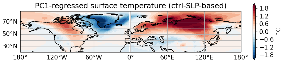
Figure A1 The positive AO pattern in the control simulations, obtained by regressing surface temperature onto the first principal component (PC1) of sea-level pressure (SLP). 20–90° N daily zonal-mean SLP anomalies in DJF are used.

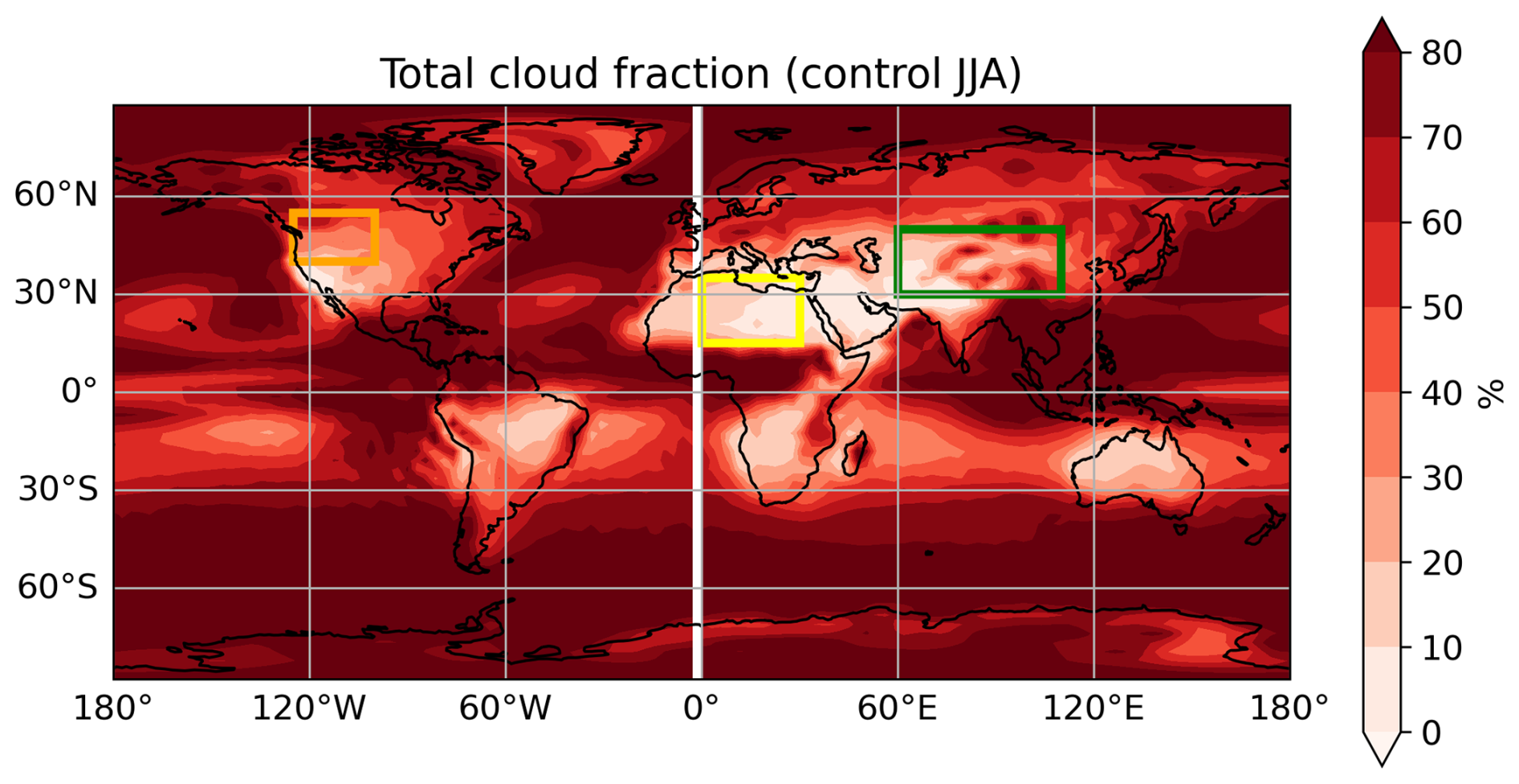
Figure A2 Total cloud fraction in JJA of the control simulations.

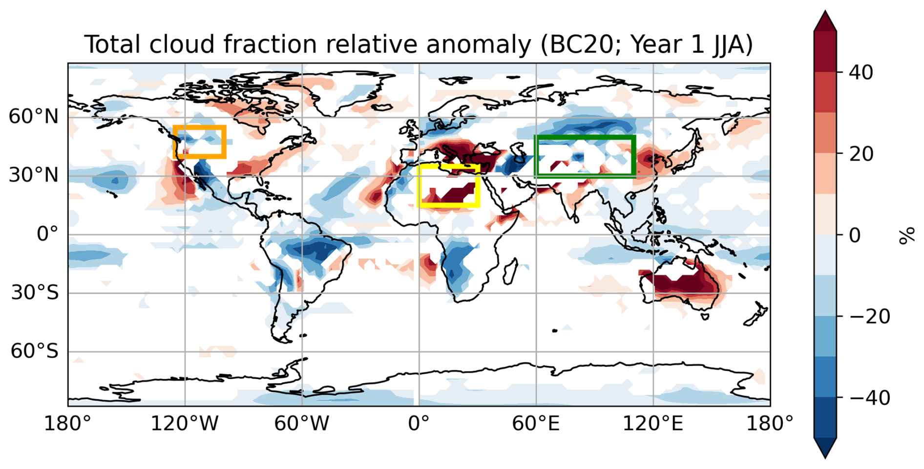
Figure A3 Percentage change of total cloud fraction in JJA of the first year for BC20. White patches indicate changes that are not significant at the 95 % confidence level using a t test.

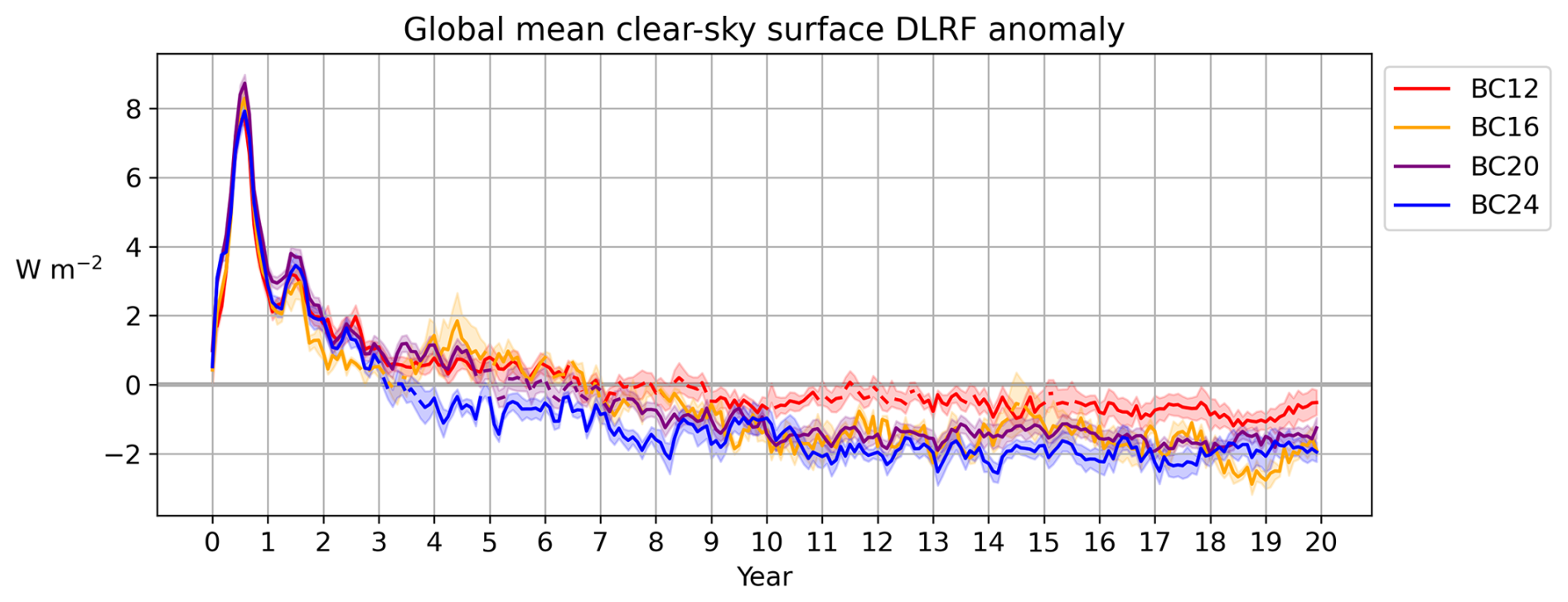
Figure A4 Monthly averaged global mean response of clear-sky surface DLRF. Shading indicates ±1 standard error of the ensemble mean. Dashed lines indicate where the standard error overlaps with the zero line.

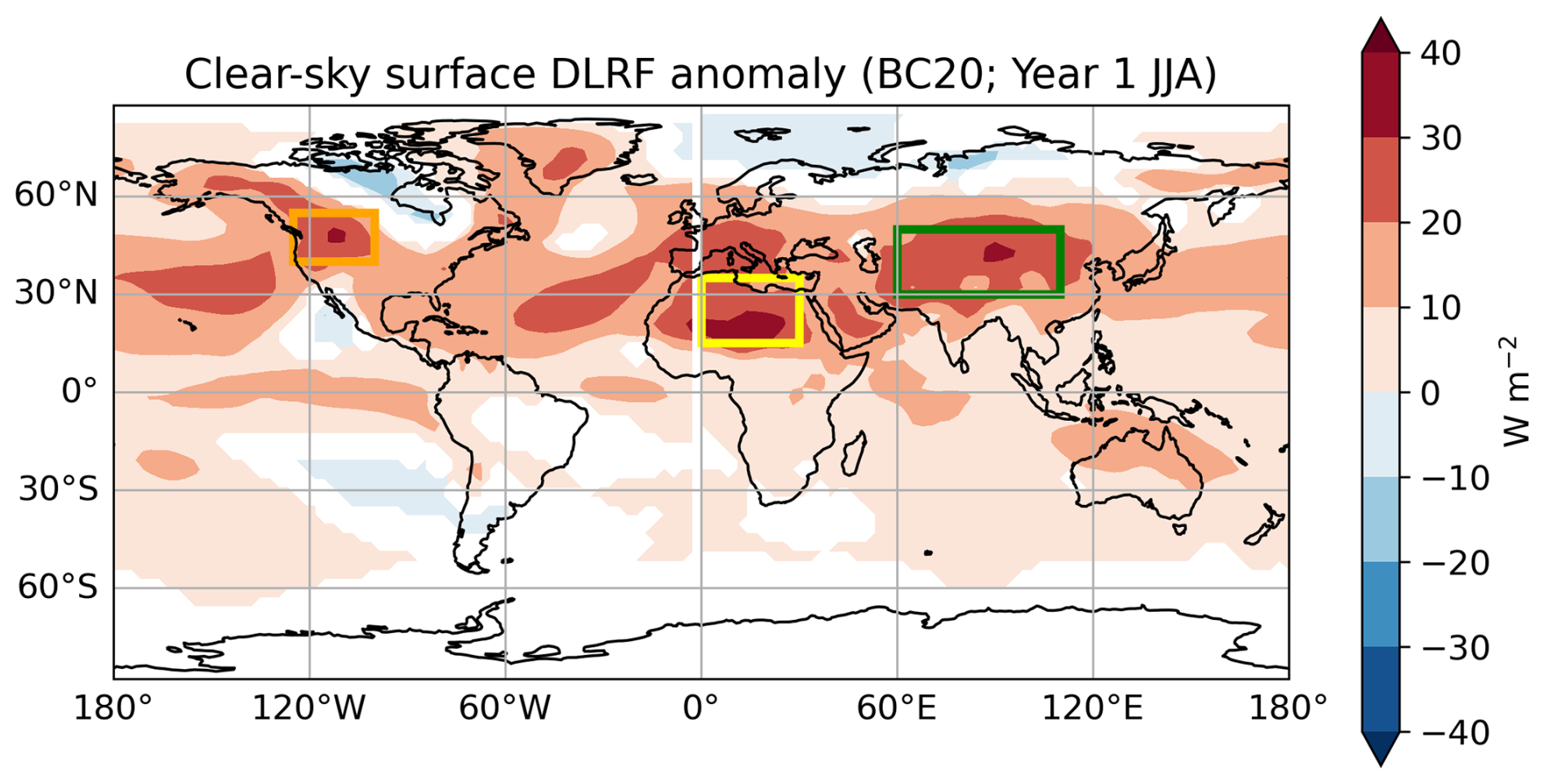
Figure A5 Response of clear-sky surface DLRF for BC20 in the first JJA. It is defined as positive downward. White patches indicate changes that are not significant at the 95 % confidence level using a t test.

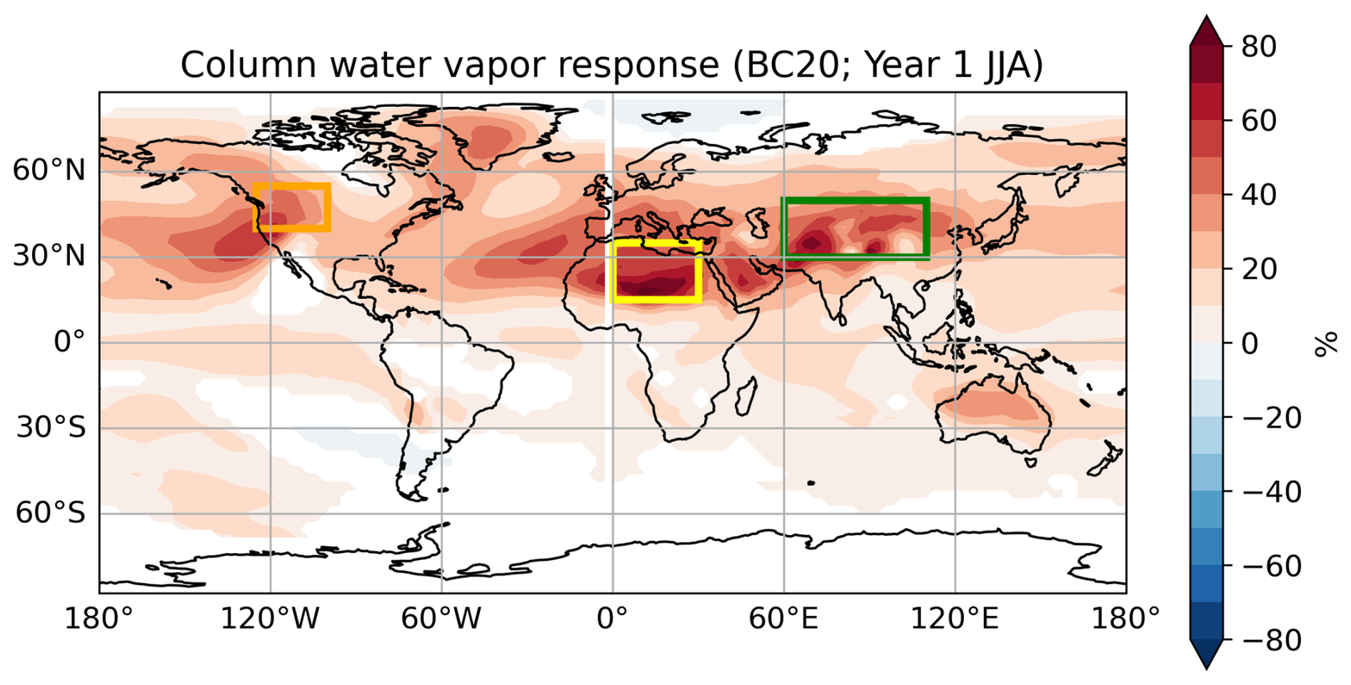
Figure A6 Response of column water vapor in JJA of the first year for BC20. White patches indicate changes that are not significant at the 95 % confidence level using a t test.

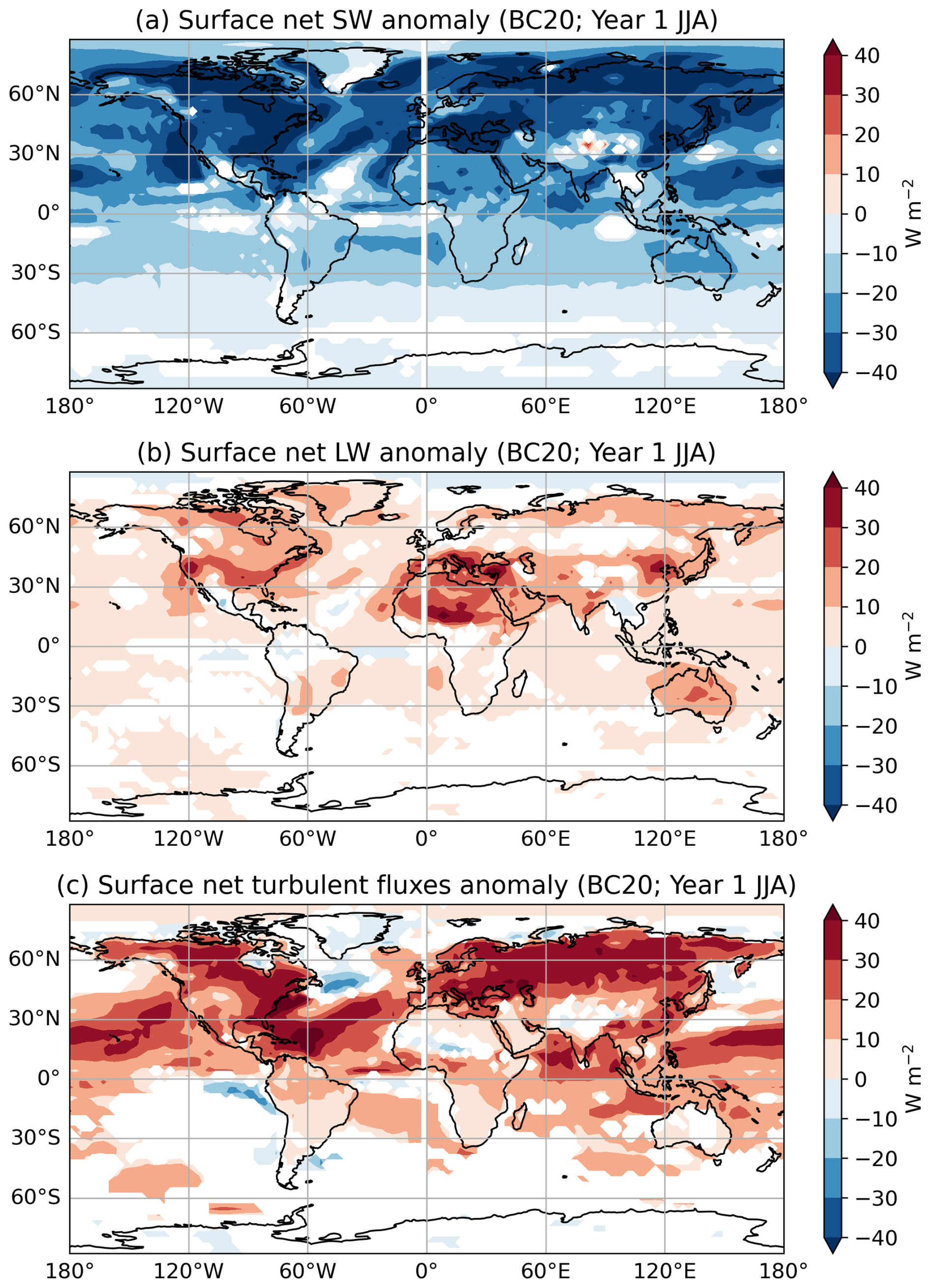
Figure A7 Responses of (a) surface net shortwave radiative flux, (b) surface net longwave radiative flux, and (c) surface net turbulent fluxes in first year JJA for BC20. The surface net energy flux response is the sum of these three responses (Fig. 6b). The fluxes are defined as positive downward. White patches indicate changes that are not significant at the 95 % confidence level using a t test.

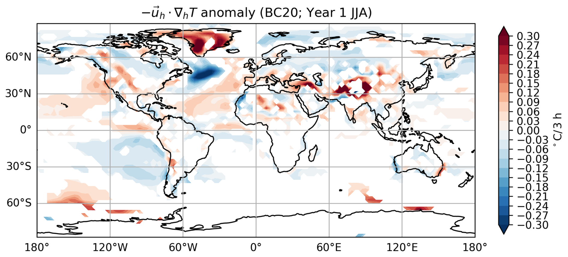
Figure A8 Temperature advection responses in JJA of the first year for BC20. The sign is defined such that positive values imply a positive local temperature tendency due to temperature advection. White patches indicate changes that are not significant at the 95 % confidence level using a t test.

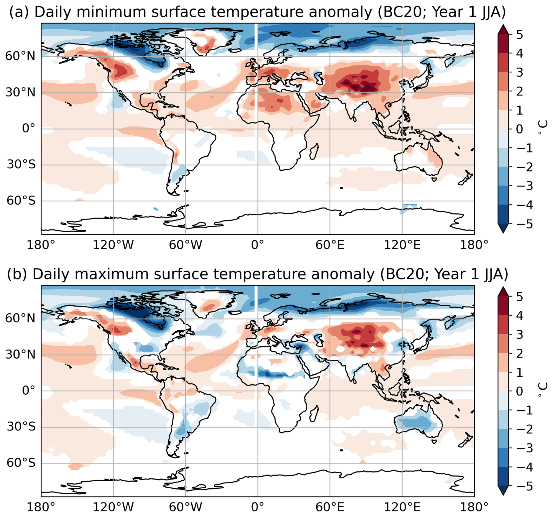
Figure A9 Responses of (a) daily minimum and (b) daily maximum surface temperature in JJA of the first year for BC20. White patches indicate changes that are not significant at the 95 % confidence level using a t test.

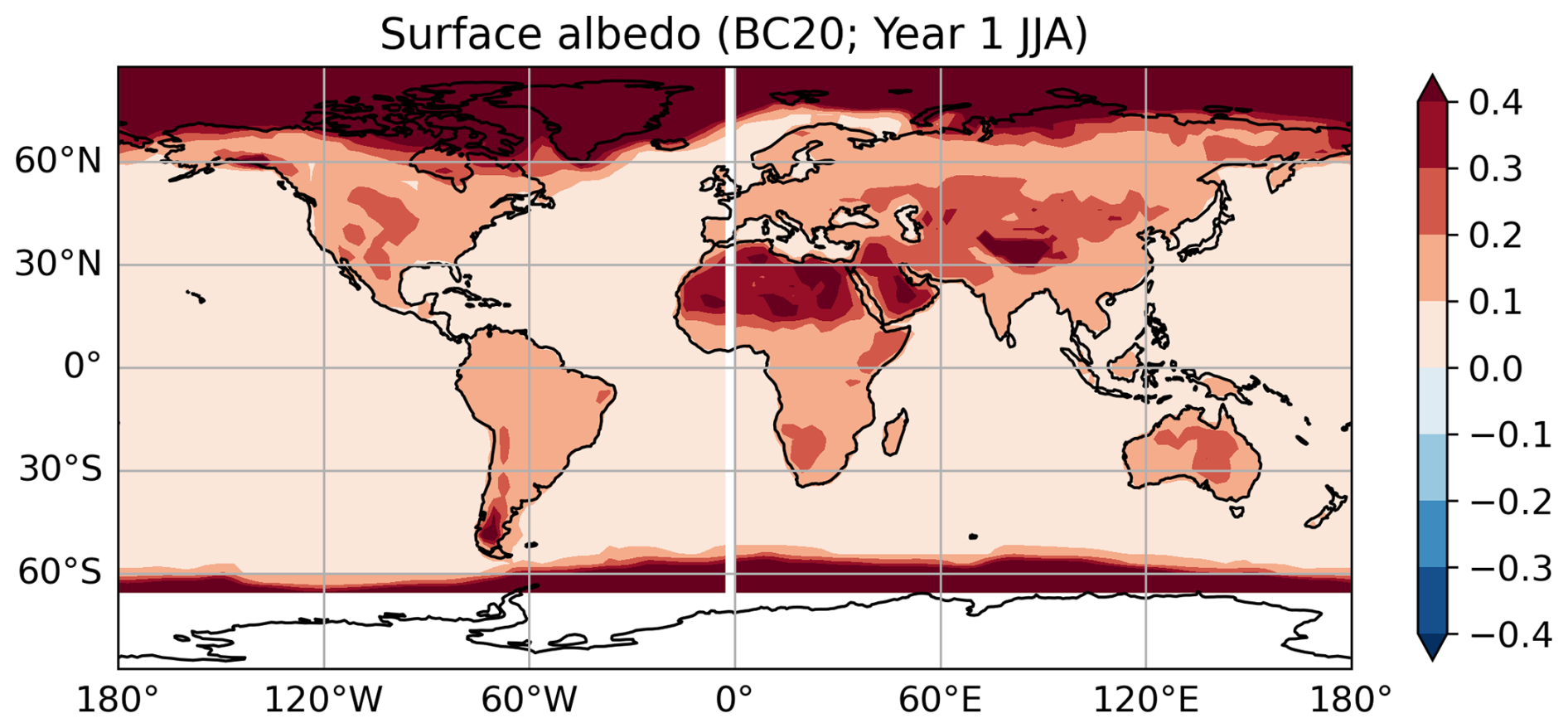
Figure A10 Surface albedo in JJA of the first year for BC20.

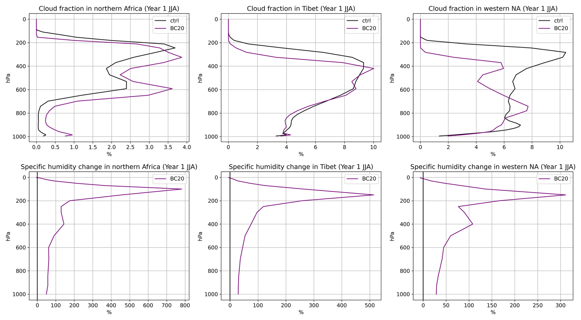
Figure A11 Vertical distributions of the cloud fraction and changes in specific humidity over the regions that experience surface warming in the first JJA. The areas of northern Africa, Tibet, and western North America correspond to the yellow, green, and orange boxes in Fig. 6a, respectively.

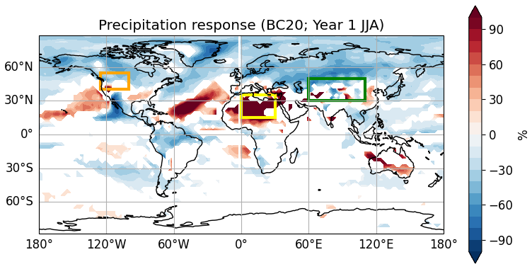
Figure A12 Response of precipitation in JJA of the first year for BC20. White patches indicate changes that are not significant at the 95 % confidence level using a t test.