Benchmarking conditioners in Liang–Kleeman Information Flow: application to land–atmosphere interactions in humid forests

The Liang–Kleeman Information Flow (LKIF) framework has been increasingly used to identify causality in Earth–system dynamics in recent years. Yet, uncertainties remain regarding how the causal graph changes when mediators and confounders (conditioners) are introduced, i.e., divergence between the bivariate and conditioned forms. A controlled synthetic experiment shows that LKIF preserves correct causal directions under hidden confounding, while differences between bivariate and multivariate estimates still occur. We characterize these differences using time-varying LKIF and introduce several quantifiers, including Conditioner Dominance Index, Moderation Gain, Conditioning Pressure, and Convergence Rate, to evaluate the contributions of conditioners. This is illustrated in an application to soil moisture (SM) and vapor pressure deficit (VPD) couplings with vegetation (leaf area index (LAI) and gross primary productivity (GPP)) in humid forest regions of Southeast China and the Amazon Basin, using satellite-derived and reanalysis data over 1981–2018. We find that the influence of SM on LAI remains consistently stable and shows little sensitivity to the selected conditioners, whereas its influence on GPP and that of VPD on vegetation exhibit substantial divergence between bivariate and multivariate estimates. This divergence peaks under compound dry–hot conditions, with VPD and temperature emerging as dominant conditioners. These results demonstrate that bivariate and multivariate LKIF can yield markedly different conclusions across time and space, especially under compound environmental stress. More importantly, even for the same variables in a causal graph, the same conditioners can affect the temporal evolution of the causal relationships very differently at different locations. This highlights how stationary assumptions may oversimplify causal structure by masking relevant temporal transitions, particularly under compound environmental stress.

1 Introduction

Land–atmosphere interactions are essential for modulating the flow of energy, water, and carbon between the surface of the land and the atmosphere, and they are especially responsive to extreme climate events. The soil–vegetation–atmosphere coupling continuum is central to these interactions, influencing and responding to changes in environmental conditions (Piao et al., 2020; Cui et al., 2020). Extreme events, like droughts and heatwaves, disrupt these interactions by depleting soil moisture (SM) and increasing vapor pressure deficit (VPD) – two key drivers of vegetation stress (Novick et al., 2016; Liu et al., 2020; Zhong et al., 2023). While SM regulates the quantity of water accessible for plant absorption (Sperry et al., 2017), VPD indicates the atmospheric demand for water, affecting plant transpiration and stomatal function (Zhou et al., 2019). The co-occurrence of restricted water supply and heightened evaporative demand during extreme conditions can significantly stress plants, leading to a decrease in photosynthesis and hindering growth (Green et al., 2019; Liu et al., 2020). This has significant implications for food and water security, especially in water-scarce regions. It is, therefore, vital to understand how vegetation responds to variations in SM (representing moisture supply) and VPD (representing moisture demand) during extreme events for assessing ecosystem vulnerability/resilience and to improve the prediction of vegetation–climate feedbacks. However, accurate predictions require observing and quantifying/representing these events to better understand them, unhindered by relative sensitivities in climate and weather models.

Most existing studies have investigated the relationships among SM, VPD, and vegetation using conventional statistical techniques such as correlation and regression (Yuan et al., 2019; Zhong et al., 2023). While these approaches can reveal co-variability, they identify symmetrical relationships that do not imply causation or directionality (Stips et al., 2016; Docquier et al., 2023). As a result, utilizing basic statistical methods makes it challenging to differentiate cause from effect. To address these limitations, several causal inference techniques, such as Granger Causality (GC) and Peter and Clark Momentary Conditional Independence (PCMCI), have been suggested to investigate complex land–atmosphere interactions (Papagiannopoulou et al., 2017; Krich et al., 2020; Dubey and Ghosh, 2023). In land–atmosphere studies, these methods have been used to infer lagged directional links among hydroclimatic and vegetation variables, to reconstruct process or causal networks, and to disentangle more direct dependencies from indirect pathways and observed common drivers; for example, information-theoretic process-network approaches have been applied to ecohydrological systems, and PCMCI has also been used to estimate biosphere–atmosphere causal networks (Ruddell and Kumar, 2009; Krich et al., 2020). Although these methods allow us to retrieve causal relationships, they continue to encounter challenges such as inconsistent or method-dependent causal estimates, strong sensitivity to assumptions (e.g., stationarity), difficulty in representing multiscale feedbacks, and limited robustness in the presence of hidden or time-varying confounders (Docquier et al., 2024; Shao et al., 2024). Recently, the Liang–Kleeman Information Flow (LKIF) has surfaced as an encouraging formalism to quantify cause–effect relationships (Liang, 2013, 2014, 2016, 2021). In land–atmosphere applications, LKIF has been used to quantify directional SM influences on precipitation and temperature, and to diagnose evolving coupling strength in nonstationary systems (Hagan et al., 2019; Liu and Pu, 2019; Sun et al., 2025; Takaya et al., 2025). The LKIF framework differs from causal measures introduced primarily through statistical association, prediction, or conditional-independence criteria because its information flow rate is derived from the entropy evolution of an underlying dynamical system (Liang, 2016). Specifically, the information flow (T_X→Y) is obtained by decomposing the rate of change of the marginal entropy of Y into the entropy tendency arising when the influence of X is instantaneously excluded and the contribution transferred from X. This derivation yields the principle of nil causality as a theorem: if the evolution law of Y is independent of X, then $T_{X\to Y}=\mathrm{0}$.

In contrast, GC and transfer entropy define influence through improved prediction, while PCMCI identifies causal links through iterative conditional-independence testing among lagged variables. LKIF provides a directional, signed rate of entropy transfer grounded in dynamical systems rather than only a measure of statistical dependence (Liang, 2016; Docquier et al., 2024). Its time-varying and multivariate extensions allow this rate to evolve through time and to be estimated while accounting for other observed variables. Nevertheless, the empirical estimator remains dependent on the assumed dynamical representation, sampling characteristics, and adequacy of the variables included in the analysis.

Originally, LKIF assumed stationarity (Liang, 2013, 2014), such that causal relationships were considered constant over time. However, in reality, interactions like vegetation–climate are fundamentally non-stationary processes, such that assuming stationarity could restrict our understanding by overlooking important temporal variations, especially when anomalous events arise. To address this issue, Hagan et al. (2019) adapted the bivariate LKIF framework to handle non-stationarity, which was further extended by Zhou et al. (2024) (Z24 hereafter) into a multivariate, nonstationary form, building on the multivariate LKIF approach by Liang (2021). Z24's multivariate approach allows for the inclusion of mediating and/or confounding variables, providing deeper insights into causal links. Here, a variable is a mediator (M) if it lies on the causal pathway between a driver X₁ and a response X₂ ($X_{\mathrm{1}}\to M\to X_{\mathrm{2}}$). Conditioning on M in the multivariate LKIF framework helps separate the direct information flow X₁→X₂ from indirect contributions transmitted through M. Meanwhile, a confounder is a variable C that influences both X₁ and X₂ (C→X₁ and C→X₂); omitting C can bias the estimated coupling by inducing a spurious information flow between X₁ and X₂. Z24 demonstrated through theoretical experiments that both the multivariate and bivariate LKIF approaches are valuable for understanding land–atmosphere interactions, even in the presence of mediators and confounders. In this study, we consider both mediators and confounders under the same terminology, i.e., “conditioners”.

While the LKIF has been successfully applied to many problems in geoscience, uncertainties remain regarding the physical limitations of using the bivariate and multivariate forms, especially when applied to land–atmosphere interactions. For instance, Z24 noted that the multivariate and bivariate forms yield similar results in the presence of external variables but did not provide conclusive criteria for when the bivariate LKIF may be compromised or less reliable, and more importantly, did not clarify the physical limitations leading to their differences. Meanwhile, Docquier et al. (2023) showed that, in a time-invariant LKIF analysis, omitting a key state variable can make bivariate and multivariate estimates diverge substantially. Furthermore, interactions in, say, the land–atmosphere continuum are tightly coupled with overlapping drivers; for example, vegetation responses may be shaped simultaneously by SM, VPD, and temperature (Novick et al., 2016; Green et al., 2017; Liu et al., 2020). In such cases, neglecting important variables could lead to inflated or misleading causal strength and variability. Moreover, the influence of these variables is not static but depends on the prevailing land–atmosphere state, where different environmental conditions shape how strongly additional variables contribute to the estimated causal relationships.

This motivates a key question which we explore in this study: under which conditions do the bivariate and multivariate LKIFs differ? More precisely, why would they differ in different locations for the same time period, or differ over time for the same location, even when the same variables are used? This raises the question of how the influence of “conditioners” varies in space and time in the causal estimation based on LKIF, especially under a nonstationary assumption. In this study, we investigate the importance of conditioners in estimating vegetation responses, based on gross primary productivity (GPP) and leaf area index (LAI), to SM and VPD using the Z24 framework. Indications from Z24 suggest that the influence of conditioners may rely on the level of dependency between the cause and the effect variables. Thus, in this study, we leverage this idea to further explore the conditions under which there would be more relevance for conditioners in the LKIF estimation. Understanding these dynamics is critical for accurately studying vegetation responses to hydroclimatic drivers.

2 Materials and Methods

2.1 Causality Formalism

The causal inference method applied here is based on the LKIF causality analysis formalism, which is rigorously derived and formulated from first principles (Liang, 2014, 2016, 2021). In this context, the causality from one time series (X₂) to another (X₁) is quantified by the rate at which information flows from X₂ to X₁. Liang (2021) extended this approach to a d–dimensional space to include the influence of potential confounding factors that may impact the relationship between X₂ and X₁. In a system with d time series, the information flow from X₂ to X₁, while accounting for conditioning variables, is expressed as (Eq. 1):

$$\begin{array}{}\text{(1)}& T_{\mathrm{2}\to \mathrm{1}|\mathrm{3},\mathrm{4},\mathrm{\dots },d}={\displaystyle \frac{\mathrm{1}}{\det \mathbf{C}}}\cdot {\sum }_{j=\mathrm{1}}^d{\mathrm{\Delta }}_{\mathrm{2}j}{\mathbf{C}}_{j,d\mathrm{1}}\cdot {\displaystyle \frac{{\mathbf{C}}_{\mathrm{12}}}{{\mathbf{C}}_{\mathrm{11}}}}\end{array}$$

where $T_{\mathrm{2}\to \mathrm{1}|\mathrm{3},\mathrm{4},\mathrm{\dots },d}$ is the LKIF from X₂ to X₁ taking into account the influence of X₃, …, X_d on X₁, C is the sample covariance matrix, and det C is its determinant. Δ_2j denotes the cofactor of C. C_j,d1 represents the sample covariance between X_j and the temporal derivative $\mathrm{d}{\dot{X}}_{\mathrm{1}}/\mathrm{d}t$ using Euler's forward differencing, C₁₂ is the sample covariance between X₁ and X₂ and C₁₁ is the sample variance of X₁ (for details see Liang, 2021).

Recently, Z24 extended Liang's multivariate information flow framework by incorporating the Kalman filter to address non–stationarity, resulting in the Multivariate Time-varying Liang–Kleeman Information Flow method. This approach allows for the dynamic tracking of causality between multiple time series variables. Within this framework, the Kalman filter estimates the covariance matrix at each time step, which is then used for calculating the time-varying causality between the system's variables. The key equation for Z24 is (Eq. 2):

$$\begin{array}{}\text{(2)}& T_{\mathrm{2}\to \mathrm{1}|\mathrm{3},\mathrm{4},\mathrm{\dots },d}\left(t\right)={\displaystyle \frac{\mathrm{1}}{\det \mathbf{P}}}\sum _{j=\mathrm{1}}^d{\dot{\mathrm{\Delta }}}_{\mathrm{2}j}{P}_{j,d\mathrm{1}}{\displaystyle \frac{P_{\mathrm{12}}}{P_{\mathrm{11}}}}\end{array}$$

where $T_{\mathrm{2}\to \mathrm{1}|\mathrm{3},\mathrm{4},\mathrm{\dots },d}$ is the LKIF from X₂to X₁ taking into account the influence of X₃, …, X_d on X₁, P is the resulting covariance matrix estimated by the Kalman filter and updated at each time step, and det P denotes its determinant. ${\dot{\mathrm{\Delta }}}_{ij}$ are the cofactors of the matrix P. And P_j,d1 are the resulting covariance between X_j and the temporal derivative $\mathrm{d}{\dot{X}}_{\mathrm{1}}/\mathrm{d}t$. P₁₂ is the covariance between X₁ and X_2, and P₁₁ is the variance of X₁ (for details, see Z24 (Zhou et al., 2024)).

In this study, the time-varying covariance matrix was estimated using a square-root Kalman filter within the Z24 framework. The Kalman gain was computed recursively within the filter from the evolving covariance estimates. The process-noise covariance matrix Q and measurement-noise covariance matrix R were estimated from the input series using a moving-window procedure. Specifically, the input vector was first smoothed using an unweighted moving average (UWMA) with a window length of 24 months, and covariance estimation was then performed over a lookback window of 90 months. The filter was initialized using the smoothed signal as the initial a posteriori state estimate and identity matrices as the initial covariance factors.

In the present implementation, the Z24 framework tracks evolving covariance structure through a Kalman-filter-based formulation and therefore relies on a linear approximation over short temporal intervals. This approximation is useful for resolving time-varying behaviour in nonstationary systems, but it may not fully represent strongly nonlinear responses. In land–atmosphere systems, such behaviour may arise under strongly varying or extreme environmental conditions. Accordingly, the inferred time-varying information flow (IF) should be interpreted in light of this approximation.

To evaluate the statistical significance of the LKIF at each time step, the information flow estimate is treated as approximately normally distributed. Its uncertainty is obtained from the maximum-likelihood parameter covariance (inverse Fisher information matrix), and the flow is considered significant when the absolute information flow exceeds the corresponding significance threshold at the chosen level. A controlled synthetic experiment demonstrating the behavior of time-varying LKIF under hidden confounding is provided in Appendix A. The results show that LKIF accurately recovers the correct causal directions and structure even as the strength of unobserved confounding increases. However, differences between bivariate and multivariate IF estimates may arise, reflecting the influence of unobserved conditioners. These findings demonstrate that, while LKIF maintains directional fidelity, conditioning is essential for isolating direct effects and avoiding misinterpretation of causal strength.

In this study, the LKIF from SM and VPD to LAI/GPP is quantified, while also accounting for the influence of multiple conditioning variables (i.e., SM/VPD, temperature (T), and surface solar radiation (SSR)). This directional focus reflects the roles of SM and VPD as terrestrial water supply and atmospheric water demand, respectively, and the study does not aim to provide an exhaustive bidirectional analysis of all variable pairs. We interpret LKIF as a signed rate of directed information transfer from a source variable to a target variable. A statistically significant nonzero LKIF indicates a directed causal influence of the source on the target, while the absolute magnitude of LKIF characterizes the strength of the directed influence. When LKIF is positive (+IF), this suggests that variability in the source increases the variability of the target. In contrast, a negative LKIF (−IF) value indicates that variability in the source decreases the variability of the target (Liang, 2014; Docquier et al., 2024).

2.2 Differential Information Flow (ΔIF) Calculation

To assess how the causal influence of individual variables (SM or VPD) on vegetation (LAI/GPP) changes in the presence of conditioners, the differential Information Flow (ΔIF) is computed. ΔIF is the signed difference between the bivariate (T^bi) and the multivariate (T^mv) IF (Eq. 3). The absolute value of this difference is given by |ΔIF|. Applied to the physical problem here (Eqs. 4–5), this metric quantifies the change in IF from SM/VPD to the vegetation (bivariate form) and its multivariate form (taking into account the influences from VPD/SM, T and SSR). Thus, ΔIF of SM and VPD is calculated using the following equations:

$$\begin{array}{}\text{(3)}& {\displaystyle }{\mathrm{\Delta }}_{\mathrm{IF}}\left(t\right)=T^{\mathrm{bi}}\left(t\right)-T^{\mathrm{mv}}\left(t\right)\text{(4)}& {\displaystyle }{\mathrm{\Delta }}_{\mathrm{SM}}\left(t\right)=T^{\mathrm{SM}\to \mathrm{LAI}/\mathrm{GPP}}\left(t\right)-T^{\mathrm{SM}\to \mathrm{LAI}/\mathrm{GPP}|\mathrm{VPD},T,\mathrm{SSR}}\left(t\right)\text{(5)}& {\displaystyle }{\mathrm{\Delta }}_{\mathrm{VPD}}\left(t\right)=T^{\mathrm{VPD}\to \mathrm{LAI}/\mathrm{GPP}}\left(t\right)-T^{\mathrm{VPD}\to \mathrm{LAI}/\mathrm{GPP}|\mathrm{SM},T,\mathrm{SSR}}\left(t\right)\end{array}$$

Based on the computed $\left|\mathrm{\Delta }\mathrm{IF}\right|$ values, we assess the conditions under which the multivariate IF diverges (converges) from (to) the bivariate form. A small $\left|\mathrm{\Delta }\mathrm{IF}\right|$ indicates that the bivariate form is very similar to the multivariate one. In such cases, the inclusion of additional variables does not notably alter the overall estimated causal influence. However, this similarity does not establish causal sufficiency or imply that individual conditioners are unimportant, because opposing pathway contributions may compensate and yield a small overall difference. Conversely, a large $\left|\mathrm{\Delta }\mathrm{IF}\right|$ suggests that the causal influence is substantially modified when additional variables are introduced, indicating a more complex causal relationship. In this case, conditioners provide additional significant information that reshapes the apparent causal structure. It is essential to note that the change in causal structure by incorporating other variables does not necessarily imply that the bivariate form is incorrect in isolating dependencies, but rather that the quantitative information gathered is not accurate. As discussed in Vannitsem et al. (2024), in a simplified setting, the addition of observables can indeed modify the amplitude or sign of the influence but not the importance of the considered variable in the causal relationship uncovered. The emergence of spurious LKIF is, however, possible as illustrated in Docquier et al. (2023).

To assess the statistical significance of the ΔIF between paired conditions (e.g., with vs. without a conditioner), a paired two-tailed Student's t-test was applied at each time step using the set of grid-cell IF estimates within the study region. A 95 % confidence interval (CI) for the difference in means was computed, and ΔIF was considered statistically significant when the CI did not include zero (equivalent to p<0.05).

To evaluate the sensitivity of this significance assessment to the choice of testing framework, we additionally performed a paired spatial block bootstrap at each monthly time step. The bivariate–multivariate IF differences were resampled using contiguous 3 × 3 grid-cell blocks, while preserving the pairing between the two estimates. This block resampling retains local spatial dependence among neighboring grid cells rather than treating individual cells as fully independent resampling units. The bootstrap-based 95 % confidence intervals identified the same significant periods as the paired t-test, and the bootstrap is therefore used here as a complementary sensitivity assessment of the t-test-based significance pattern.

Because significance was assessed repeatedly across monthly time steps, we further applied the Benjamini–Hochberg false discovery rate (FDR) procedure to the resulting monthly p-values to control the expected proportion of false discoveries associated with multiple testing (Benjamini and Hochberg, 1995; Wilks, 2016). The FDR correction did not alter the temporal pattern of significant ΔIF.

The bootstrap is performed separately at each monthly time step, with the spatial ensemble of grid cells providing the resampling dimension; temporally successive observations are therefore not treated as independent bootstrap replicates. Nevertheless, successive IF estimates may retain temporal dependence because they are derived from temporally filtered series. In addition, spatial block resampling retains local dependence among neighboring grid cells but may not fully capture longer-range spatial dependence. The resulting confidence intervals may show some sensitivity to the assumed block size. These confidence intervals should therefore be interpreted as approximate regional uncertainty bounds rather than exact pointwise significance tests.

2.3 Information-based Correlations (rIF)

In some cases, large differences may exist between the multivariate and bivariate forms; however, the correlations between their time-varying estimates could be very high, implying that they capture the same physical process but at different magnitudes. Therefore, we also assess the Pearson correlation (rIF) between the time-varying bivariate IF and the time-varying multivariate one. This allows us to obtain a more holistic view of the conditions for divergence between the bivariate and multivariate IFs. For regime-specific behavior, rIF is restricted to the subset of months belonging to a defined regime (Eq. 6):

$$\begin{array}{}\text{(6)}& \mathrm{rIF}=\left|\mathrm{corr}\right(T_{\mathrm{bi}}\left(t\right),T_{\mathrm{mv}}\left(t\right){)}_{\mathrm{regime}}|\end{array}$$

In this study, we use the absolute correlation (|rIF|), focusing on the strength of the temporal covariation. Here, we bin the time series of SM and VPD into four quantile-based regimes, yielding a 4×4 grid of combined regimes, corresponding to the combinations of SM and VPD quartiles (Q1, Q2, Q3, Q4 for each). The SM quartiles range from Q1, representing the driest conditions, to SM at Q4, representing the wettest conditions. Meanwhile, VPD quartiles range from Q1 (lowest demand) to Q4 (highest demand). For each quartile, we calculate rIF and the median of |ΔIF|. Quartiles were selected as a practical compromise between resolving hydroclimatic gradients and retaining sufficient samples within each joint SM–VPD regime. Terciles provide a coarser partition that can obscure intermediate state dependence, whereas quintiles increase sparsity in some regime combinations (Fig. S4).

2.4 Conditioner-Based Decomposition of Information Flow Divergence

Understanding why T^mv diverges from T^bi leads us to derivable measures to quantify the relevance of the conditioners. To determine how individual conditioners, modify the inferred causal influence between each driver–target pair, the differential Information Flow signal ΔIF(t) was decomposed into contributions (Eqs. 7–9) from progressively expanded conditioning sets. Let T^bi(t) denote the bivariate IF from the driver (SM or VPD) to the target variable (LAI or GPP) and let T^mv|m(t) denote the corresponding multivariate IF conditioned on a conditioner set $(m_{\mathrm{1}},m_{\mathrm{2}},m_{\mathrm{3}})$. For a coupling and a sequence of conditioners, the decomposition follows,

$$\begin{array}{}\text{(7)}& {\displaystyle }\mathrm{\Delta }\mathrm{IF}{m}_{\mathrm{1}}\left(t\right)=T^{\mathrm{bi}}\left(t\right)-T^{\mathrm{bi}}\left|m_{\mathrm{1}}\right(t)\text{(8)}& {\displaystyle }\mathrm{\Delta }\mathrm{IF}{m}_{\mathrm{2}}\left(t\right)=T^{\mathrm{bi}}\left|m_{\mathrm{1}}\right(t)-T^{\mathrm{bi}}|m_{\mathrm{1}},m_{\mathrm{2}}\left(t\right)\text{(9)}& {\displaystyle }\mathrm{\Delta }\mathrm{IF}{m}_{\mathrm{3}}\left(t\right)=T^{\mathrm{bi}}|m_{\mathrm{1}},m_{\mathrm{2}}(t)-T^{\mathrm{bi}}|m_{\mathrm{1}},m_{\mathrm{2}},m_{\mathrm{3}}\left(t\right)\end{array}$$

This decomposition allows us to examine which conditioner contributes most to the divergence, and in what direction. From here, we summarize how each conditioner contributes to the restructuring of Information Flow based on four indices (Eqs. 10–13) computed from the temporal components Δ IFm(t). To assess the order sensitivity of the sequential decomposition, we repeated the analysis across all permutations of the conditioner-entry order for each pathway. The results for the individual permutations are shown in Fig. S8, while their mean values and corresponding minimum–maximum ranges are summarized in Fig. S9.

In this study, we introduce four diagnostic indices: Conditioner Dominance Index (CDI), Moderation Gain (MG), Conditioning Pressure (CP), and Convergence Rate (CR), to characterize complementary aspects of divergence between bivariate and multivariate IF. These indices are derived from the sequential decomposition of ΔIF and together provide a unified description of how conditioning variables modify the inferred coupling. Specifically, MG and CP represent the positive and negative components of the decomposition, corresponding to decreases and increases in the inferred IF after conditioning, respectively, while CDI quantifies the relative contribution of each conditioner to the total magnitude of restructuring. CR, in contrast, summarizes the overall degree of agreement between the bivariate and fully conditioned estimates.

2.4.1 Conditioner Dominance Index (CDI)

The Conditioner Dominance Index (CDI) quantifies the relative contribution of the conditioner (m) to the total magnitude of information flow restructuring (Eq. 10):

$$\begin{array}{}\text{(10)}& {\mathrm{CDI}}_{\mathrm{m}}={\displaystyle \frac{{\sum }_t\left|\mathrm{\Delta }{\mathrm{IF}}_m\right(t\left)\right|}{{\sum }_{\stackrel{\mathrm{´}}{m}}{\sum }_t\left|\mathrm{\Delta }{\mathrm{IF}}_{\stackrel{\mathrm{´}}{m}}\left(t\right)\right|}}\end{array}$$

Large CDI_m values identify conditioners that dominate the divergence between bivariate and multivariate couplings.

2.4.2 Moderation Gain (MG)

Moderation Gain (MG) shows how strongly the IF decreases after including the conditioner (m). The gain is defined as (Eq. 11);

$$\begin{array}{}\text{(11)}& {\mathrm{MG}}_m={\sum }_t\max \left(\mathrm{0},\mathrm{\Delta }{\mathrm{IF}}_m\left(t\right)\right),\end{array}$$

High MG_m values indicate that the IF before inclusion of the conditioner is higher than the corresponding IF after conditioning.

2.4.3 Conditioning Pressure (CP)

Conditioning Pressure (CP) measures how strongly the IF increases after including conditioner (m) and is given in Eq. (12);

$$\begin{array}{}\text{(12)}& {\mathrm{CP}}_m={\sum }_t\max (\mathrm{0},-\mathrm{\Delta }{\mathrm{IF}}_m(t\left)\right)\end{array}$$

Large CP_m values indicate that conditioning increases the inferred IF.

2.4.4 Convergence Rate (CR)

Convergence Rate (CR) quantifies how often the bivariate estimate is close to the fully conditioned estimate. We define the CR using the absolute divergence threshold ϵ_abs (Eq. 13);

$$\begin{array}{}\text{(13)}& \mathrm{CR}={\displaystyle \frac{\mathrm{1}}{N}}{\sum }_t^N\left(\right|\mathrm{\Delta }\mathrm{IF}\left(t\right)|\le {\mathit{ϵ}}_{\mathrm{abs}})\end{array}$$

Here ϵ_abs is chosen as a fixed tolerance reflecting a physically meaningful scale of information-flow variation (e.g. the 10th percentile of ΔIF across all couplings). High CR values indicate that the bivariate coupling is sufficiently close to the multivariate form during a large fraction of the analyzed period. In the main analysis, CR was computed using ϵ_abs=0.02; a threshold-sensitivity analysis using alternative fixed tolerances is shown in Fig. S7.

2.5 Data

The gross primary productivity (GPP) data, reflecting photosynthetic activity of plants, and leaf area index (LAI), representing vegetation greenness, utilized in this study, are obtained from the Global Land Surface Satellite (GLASS) dataset (Liang et al., 2021). Both the LAI and GPP datasets cover the period 1981–2018 and have a spatial resolution of 0.05° and a temporal resolution of 8 d. For consistency with other variables in the analysis, the datasets are resampled to a spatial resolution of 0.25° × 0.25° (longitude × latitude) using bilinear interpolation and then aggregated to monthly timescales. The monthly data on volumetric soil moisture, 2 m air temperature, and surface solar radiation used in this study are obtained from the European Centre for Medium-Range Weather Forecasts' (ECMWF) datasets, with soil moisture taken from ERA5-Land and temperature and SSR from ERA5 global atmospheric reanalysis products. The weighted average of soil moisture, computed between 0 and 289 cm (all four layers of soil moisture), is used here, with the weights corresponding to the thickness of each layer (0–7, 7–28, 28–100, and 100–289 cm). The original resolution of the soil moisture data (0.1° × 0.1°) is subsequently re-gridded at a horizontal resolution of 0.25° × 0.25°. Vapor pressure deficit (VPD) is estimated using ERA5's 2 m minimum and maximum temperature and 2 m dewpoint temperature (Upreti and Ojha, 2017). The monthly anomalies for all variables are computed over the corresponding analysis periods by subtracting the respective climatological means from the original data. To ensure temporal consistency with the vegetation records, these variables are used over the period from 1981 to 2018.

LKIF estimation is performed from 1981 to 2018 for both the LAI- and GPP-based analyses. However, given the uncertainties associated with the earlier vegetation products and to ensure adequate preceding observations for the Kalman filter estimation, only the results from 2004 to 2018 are presented and interpreted in this study.

3 Results

3.1 Real-world applications in land–atmosphere interactions

Figure 1 illustrates the information flow from SM/VPD to LAI (panels a–b) and from SM/VPD to GPP (panels c–d), estimated via LKIF, for two humid forest biomes: Southeast China (114.25–117.25° E, 25.25–28.25° N) and the Amazon Basin (54–60° W, 10–15° S), over the period from 2004 to 2018. The locations of these study regions are shown in Fig. S1. Across both regions, the LKIF analysis captures the temporal evolution of vegetation response to hydroclimatic variability and reveals when conditioning on other variables (VPD, T, SSR) alters or preserves the estimated causal pathways. The results presented in this study are based on these two humid forest regions; however, they hold broader lessons that are relevant to stationary assumptions and the inclusion of conditioners in LKIF.

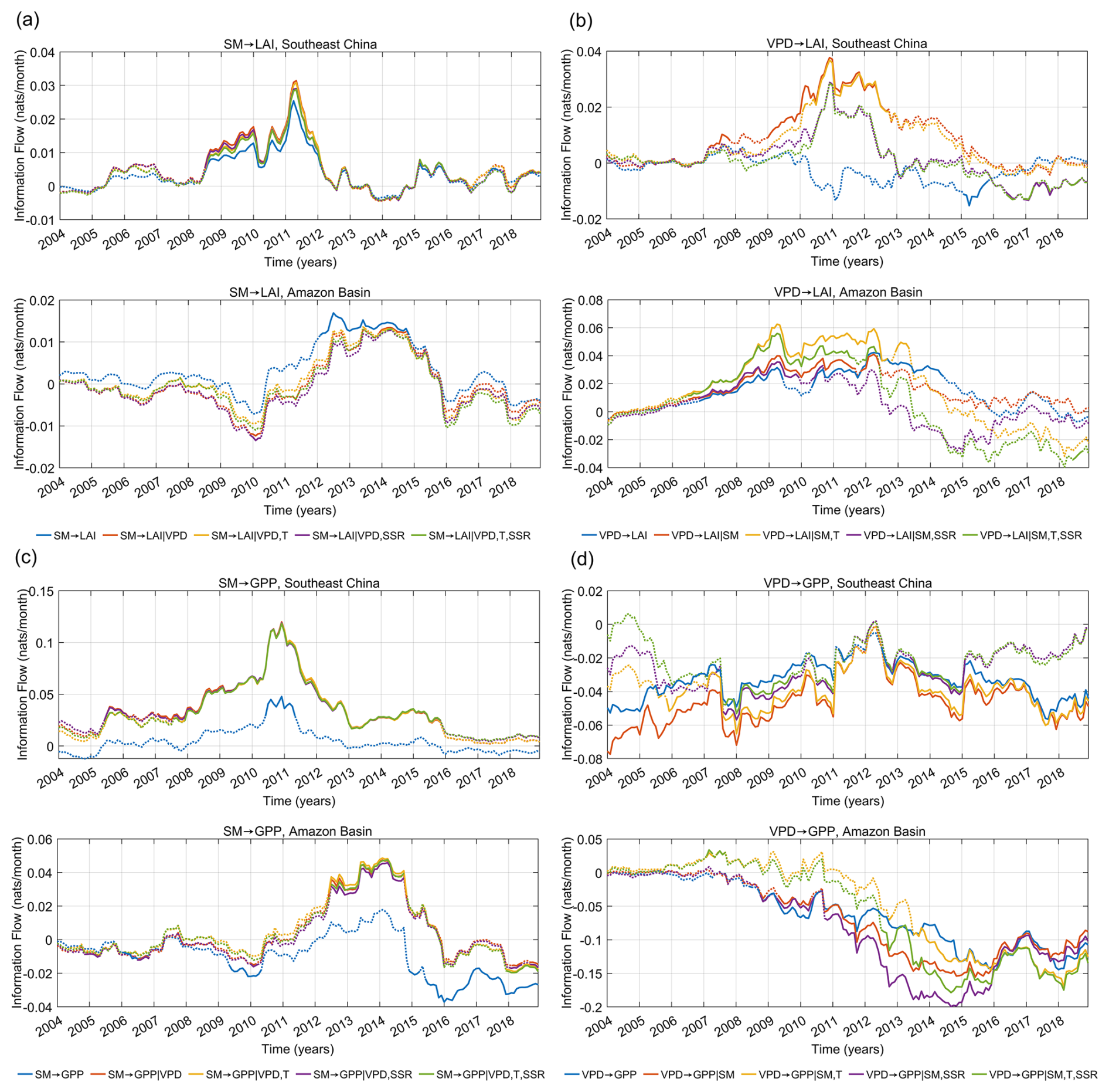
Figure 1 Time series of the information flow for Southeast China and the Amazon Basin (2004 to 2018) for both bivariate and multivariate forms. Each lettered panel contains two regional subpanels, with Southeast China shown above and the Amazon Basin below. (a) From SM to LAI, (b) From VPD to LAI, (c) From SM to GPP, (d) From VPD to GPP. Dotted lines represent the overall IF, while solid lines indicate statistically significant IF. (LAI = Leaf Area Index, GPP= Gross Primary Productivity, SM= Soil Moisture, VPD = Vapor Pressure Deficit, T= Temperature, SSR = Surface Solar Radiation).

3.1.1 Role of Conditioners in the Couplings between Soil Moisture/Vapor Pressure Deficit and Vegetation

In the Southeast China region (Fig. 1a, top panel), the SM → LAI coupling is weak and mostly insignificant during 2004–2008. From 2008 onward, the IF increased noticeably, peaking in 2011 with significant positive IF, demonstrating the increasing importance of SM for the structural variability of vegetation during this period. Conditioning on other variables (SM → LAI | VPD; SM → LAI | VPD, T; SM → LAI | VPD, SSR; SM → LAI | VPD, T, SSR) produces only minor changes in magnitude, showing that the bivariate signal is not strongly conditioned by the atmospheric factors used here because the SM influence dominates. The overall positive IF suggests that variability in SM tends to increase LAI variability in the region.

In the Amazon Basin (Fig. 1a, bottom panel), the SM → LAI pathway shows broadly similar temporal variability in both the bivariate and multivariate estimates, indicating a generally strong hydrological influence on canopy structure. However, the bivariate estimate remains larger than the multivariate estimates throughout the whole period (except in 2014–2015, when values are very similar), indicating the conditioning influence of other drivers. From 2004 to 2009, IF gradually declined toward negative values with a small fluctuation in 2007, suggesting a tendency for variability in SM to reduce vegetation structural variability, though IF remains statistically insignificant throughout this period. Between 2010 and 2014, IF increased sharply, indicating a shift towards heightened vegetation structural variability driven by moisture variability. The bivariate IF becomes significant after 2012, reflecting an apparent strengthening of the SM → LAI relationship. However, after conditioning (SM → LAI | VPD; SM → LAI | VPD, T; SM → LAI | VPD, SSR; SM → LAI | VPD, T, SSR), this significance disappears. The loss of significance indicates an overestimation of the directional coupling in the bivariate form. In the years after 2014, the IF decreases, suggesting that the influence of SM on LAI variability becomes less pronounced. Accounting for the conditioners results in only minor adjustments to IF magnitude, showing that removing atmospheric influences does not substantially alter the SM → LAI coupling. Overall, although atmospheric variables exert secondary effects, soil moisture remains the primary driver of canopy structural variability.

Figure 1b shows the VPD → LAI IFs in the two regions. The top and bottom panels show rather different temporal behaviors in the bivariate and multivariate IFs compared to Fig. 1a. In this case, introducing conditioning variables (VPD → LAI | SM; VPD → LAI | SM, T; VPD → LAI | SM, SSR; VPD → LAI | SM, T, SSR) substantially modifies the coupling behavior. However, this behavior remains time-dependent, after 2007, conditioning on the other variables leads to a stronger modification, with the divergence between the bivariate and multivariate forms increasing in both regions. In Southeast China, we even find different IF signs between the bivariate and multivariate forms from 2010 to 2016. From 2016 onwards, both regions show greater variability in IF signs across the multivariate forms. These suggest more complex VPD-driven couplings for vegetation structure than SM-driven couplings. Some of these sign differences may reflect conditioning effects, although under strongly nonlinear environmental transitions, they may also be influenced by the linear approximation underlying the present Z24 implementation.

Figure 1c–d show IFs of SM/VPD to GPP, and their multivariate forms for both regions. For the SM → GPP coupling, conditioning produces a pronounced change in Southeast China (Fig. 1c, top panel). The bivariate SM → GPP IF is statistically significant in only 13 out of the 180 months (7.2 %), whereas conditioning on VPD increases the number of significant months to 116 (64.4 %). Conditioning on VPD and T, or VPD and SSR, or VPD, T and SSR also provides a large number of significant months (105, 115 and 105 months, respectively; Table S1). Thus, conditioning substantially modifies the inferred SM → GPP coupling in Southeast China, particularly the frequency with which the estimated IF is statistically significant (Supplement Sect. S1). In contrast, the Amazon Basin (Fig. 1c, bottom panel) shows a decrease in the number of significant SM → GPP months, from 73 out of 180 months (40.6 %) in the bivariate form to 41 months (22.8 %) in the fully conditioned form (Table S2 in the Supplement). This contrasting behavior indicates that the influence of conditioners on the SM → GPP coupling is region-dependent, even when the same set of variables is considered. Pronounced differences between the bivariate and multivariate estimates are also observed for the VPD → GPP couplings (Fig. 1d), showing their greater sensitivity to the selected conditioning variables. These results reveal that dependency on conditioners is both spatially and temporally sensitive, given the same variables. The changes towards positive or negative IF are strongly impacted by ecosystem stress, here more consistent with drought occurrences in the region (Sun and Yang, 2012; Feldpausch et al., 2016). These results reveal that dependency on conditioners is both spatially and temporally sensitive, given the same variables. Thus, the influence of conditioning variables should not be assumed to remain stationary across time or space.

To assess whether the temporal evolution of LKIF could be attributed to changes in the underlying variable variances, we additionally evaluated the time-resolved means and variances of all variables included in the analysis (SM, VPD, LAI, GPP, T, and SSR; Fig. S2). Although some periods show co-variation between LKIF and individual-variable variance, no consistent correspondence is observed across pathways, time, and regions. This indicates that changes in individual variances alone do not explain the temporal evolution of LKIF.

3.2 When are Conditioners Important? Δ-Information-Flow Analysis

To further explore the conditions under which greater divergence/convergence (large/small ΔIF) between bivariate and multivariate estimates occurs in the application above, we further analyze the temporal evolution of ΔIF for both SM/VPD → LAI and the SM/VPD → GPP pathways across Southeast China and the Amazon Basin. ΔIF indicates the degree of convergence/divergence between the bivariate and multivariate IFs. Here, for the multivariate form, we include all confounding variables used in this study. Figure 2a, d show the ΔIF of SM/VPD → LAI (ΔSM: blue plots, ΔVPD: red plots), and Fig. 2g, j shows the same as Fig. 2a, d but for GPP. Figure 2a, d consistently shows high convergence in ΔSM in both regions across all times, while ΔVPD shows more time-dependent divergence. The ability of the Z24 to capture immediate changes in IF plays a pivotal role in shaping these differences. These results indicate strong similarity between the bivariate and multivariate SM → LAI coupling, as ΔSM is very small, with negligible influence from conditioners, reflecting a strong hydrological control on canopy structure in these biomes. In contrast, ΔVPD exhibits marked fluctuations and alternates between positive and negative phases. Generally, atmospheric water demand (VPD) would depend on land water supply (SM), clear skies (increased SSR), and how these increase or decrease T, to impact vegetation density (Ficklin and Novick, 2017; Yuan et al., 2019; Zhou et al., 2019). Furthermore, VPD is very sensitive to changes in these conditioners, especially the atmospheric ones, making it more responsive to their impacts. This sensitivity explains why conditioning on these variables changes the apparent strength of VPD's impact, thereby correcting bivariate bias and providing a more refined IF estimate. The GPP effect-based ΔIF shows largely different patterns compared to the LAI effect-based ΔIF. Firstly, while Fig. 2a, d show consistently convergent patterns across the whole time period for ΔSM in both regions, we find time-varying changes in ΔSM in Fig. 2g, j, although this is more distinct in Southeast China than in the Amazon Basin. This implies that SM → LAI shows greater bivariate–multivariate similarity than SM → GPP. On the other hand, ΔVPD shows rather different patterns across both regions. In Southeast China, ΔVPD shows continuously high convergence during most of the time period; however, as with ΔSM, it is characterized by fluctuations and alternates between positive and negative phases. Thus, VPD → GPP coupling shows greater similarity between the bivariate and multivariate estimates in Southeast China than in the Amazon Basin.

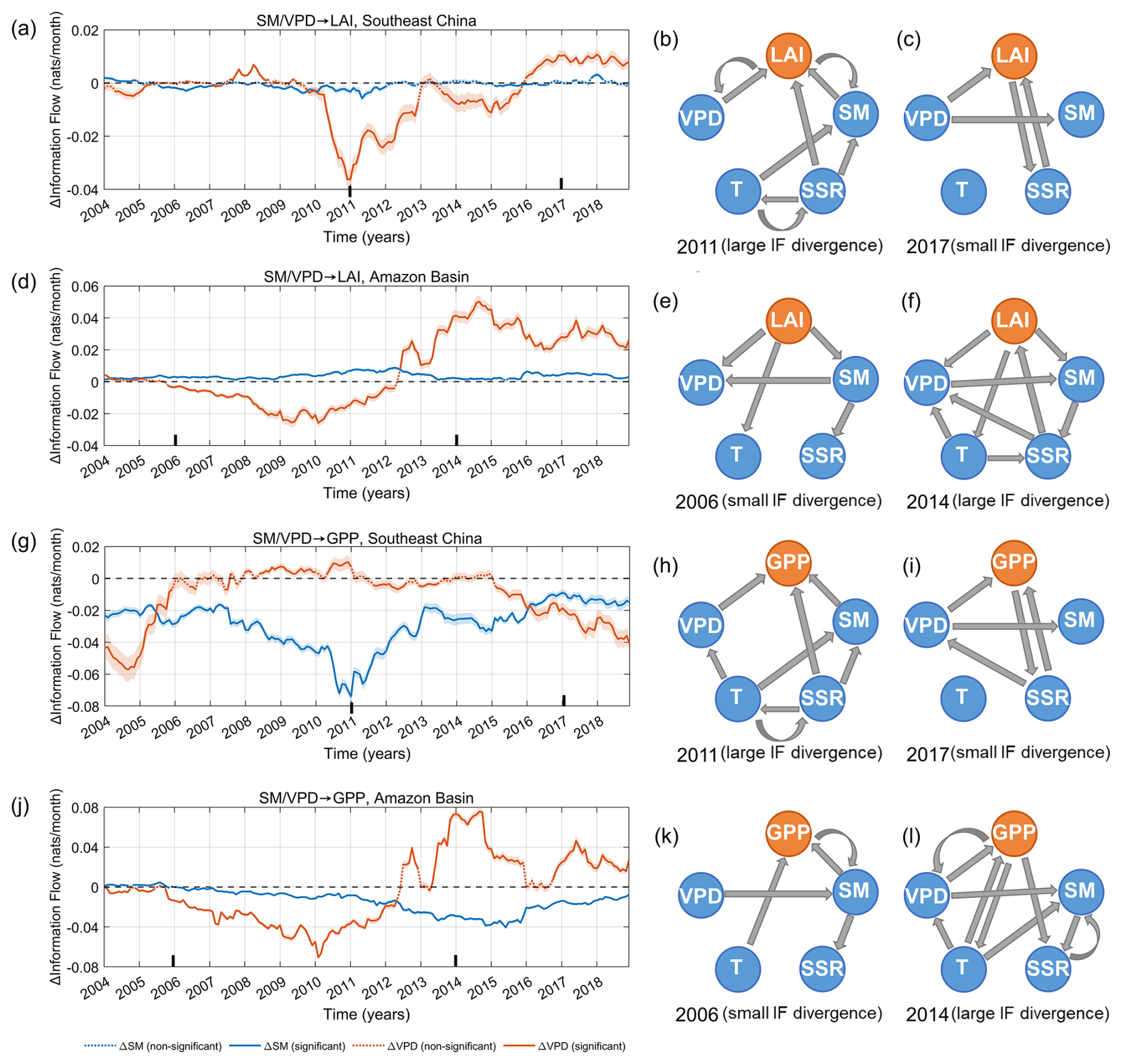
Figure 2 Time series of differential Information Flow (ΔIF) for Southeast China and the Amazon Basin (2004–2018). (a, d) for SM/VPD to LAI, and (g, j) from SM/VPD to GPP. Solid lines denote periods where ΔIF is statistically significant (p< 0.05); dotted lines indicate non-significant values. Shaded bands represent the 95 % confidence intervals. (ΔSM = $T_{\mathrm{SM}\to \mathrm{LAI}/\mathrm{GPP}-\mathrm{TSM}\to \mathrm{LAI}/\mathrm{GPP}|\mathrm{VPD}}$, T, SSR and ΔVPD = $T_{\mathrm{VPD}\to \mathrm{LAI}/\mathrm{GPP}-\mathrm{TVPD}\to \mathrm{LAI}/\mathrm{GPP}|\mathrm{SM}}$, T, SSR). Vertical tick marks on the x axes denote the time points selected for causal graph construction. Summary of the causal graphs for years exhibiting large and small IF divergence for LAI (b–c, e–f), and for GPP (h–i, k–l). The selected years are annotated in each panel according to the magnitude of IF divergence (ΔIF), indicating whether the bivariate and multivariate estimates strongly diverge or converge. Stronger ΔIF corresponds to years with richer coupling and feedback structure, whereas smaller ΔIF reflects periods with fewer couplings/feedback. The causal graphs are constructed from the corresponding five-variable multivariate estimates. (LAI = Leaf Area Index, GPP = Gross Primary Productivity, SM= Soil Moisture, VPD = Vapor Pressure Deficit, T= Temperature, SSR = Surface Solar Radiation).

Figure 2a, d, g, j show that regions with rich/strong coupling/feedback, particularly the Amazon Basin, exhibit large differences in ΔIF, indicating substantial divergence between the bivariate and multivariate pathways.

To dig deeper into the potential reasons for these nuanced patterns of ΔIF, we illustrate the causal graphs for (1) a time point where ΔIF is large (stronger divergence) and (2) a time point where ΔIF is small (stronger convergence) for both regions (Fig. 2b–c, e–f, h–i, k–l). The results suggest that stronger divergence is associated with richer coupling/feedback time points, while stronger convergence occurs when there are fewer couplings. These results agree with a previous study, which suggested that couplings/feedback reduce under drought conditions (Ruddell and Kumar, 2009). This could also explain why ΔVPD converges in Southeast China around the neighborhood time of 2011, since these periods were marked by recurrent droughts in the region (Sun and Yang, 2012). Under such drier conditions, VPD becomes a more dominant driver of vegetation, consistent with the findings of a recent study (Yuan et al., 2019). These results illustrate how ΔIF variability translates into shifts in the underlying causal structure. High-ΔIF years correspond to more complex, conditioner-driven pathway configurations, whereas low-ΔIF years reflect simpler causal structure with fewer couplings.

The selected time points were chosen to illustrate contrasting cases of pronounced large and small |ΔIF|. For the large-|ΔIF| cases, the selection also considered the documented hydroclimatic and ecological conditions during the corresponding periods. In Southeast China, the selected 2011 period coincided with the persistent and severe winter–spring drought reported by Sun and Yang (2012). In the Amazon, the selected 2014 time point occurred during a period in which changes in forest recovery dynamics have been reported, with Van Passel et al. (2024) identifying an increasing critical-slowing-down trend from around 2014 onward and relating slowing-down patterns to increased drought occurrence. The selected graphs are intended as illustrative examples of contrasting ΔIF conditions rather than statistically representative composites of all high- and low-|ΔIF| periods. Because the presence, direction, and strength of individual causal links vary through time, combining multiple periods into a composite graph could average or obscure distinct and potentially opposing causal links.

The causal graphs are obtained from the corresponding five-variable multivariate systems and therefore also contain directional influences other than the SM/VPD → LAI/GPP pathways examined in detail here. These additional links are shown to illustrate the broader causal structure at the selected time points but are not analyzed individually in the present study. Further analyses will be required to systematically disentangle these additional directional connections.

3.3 State-Dependent Patterns of Changes in Information Flow

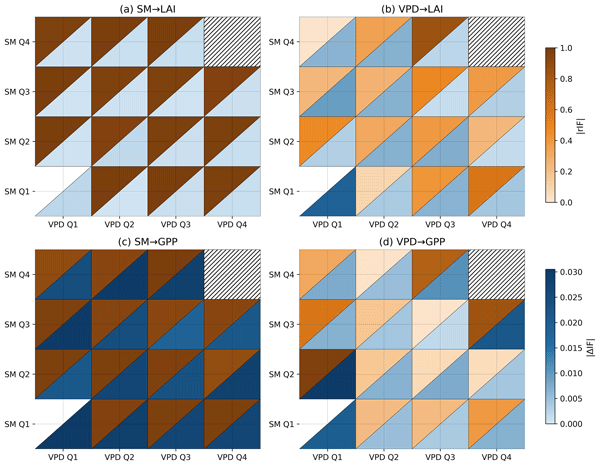
To further assess when and where bivariate and multivariate IF estimates diverge, we computed the absolute differential information flow (|ΔIF|, Sect. 2.2) and the information-based correlation (|rIF|, Sect. 2.3). To jointly visualize the two diagnostics across the combined regimes, we use the split-triangle heatmap layout. For each 4×4 panel, we overlay grid lines, label the axes by SM and VPD quartiles, and hatch any cells with zero samples using diagonal stripes; this immediately flags regimes where no robust causal inference is possible. This is routinely repeated for all four couplings, focusing on southern China, to show how |ΔIF| and |rIF| between bivariate and multivariate IF depend jointly on SM and VPD regimes.

The SM → LAI pathway (Fig. 3a) exhibits uniformly high |rIF| and low |ΔIF| across nearly all SM–VPD quartile combinations. This concentrated pattern demonstrates that the SM–LAI coupling has consistently minimal differences between bivariate and multivariate IF estimates. The uniformity across hydroclimatic states indicates that vegetation structural responses to soil moisture in humid forests are stable and largely insensitive to atmospheric variables. In contrast, the SM → GPP (Fig. 3c) shows high correlation and larger |ΔIF| values. Although the SM–GPP coupling remains strong across quartiles (as revealed by the large correlation), the pronounced difference in information flow between the bivariate and multivariate forms indicates that conditioner inclusion alters the estimated causal strength more substantially than in the SM → LAI case. This reflects the higher complexity of productivity (GPP) responses relative to canopy structure (LAI); GPP integrates more processes and is therefore more sensitive to the removal of atmospheric confounding.

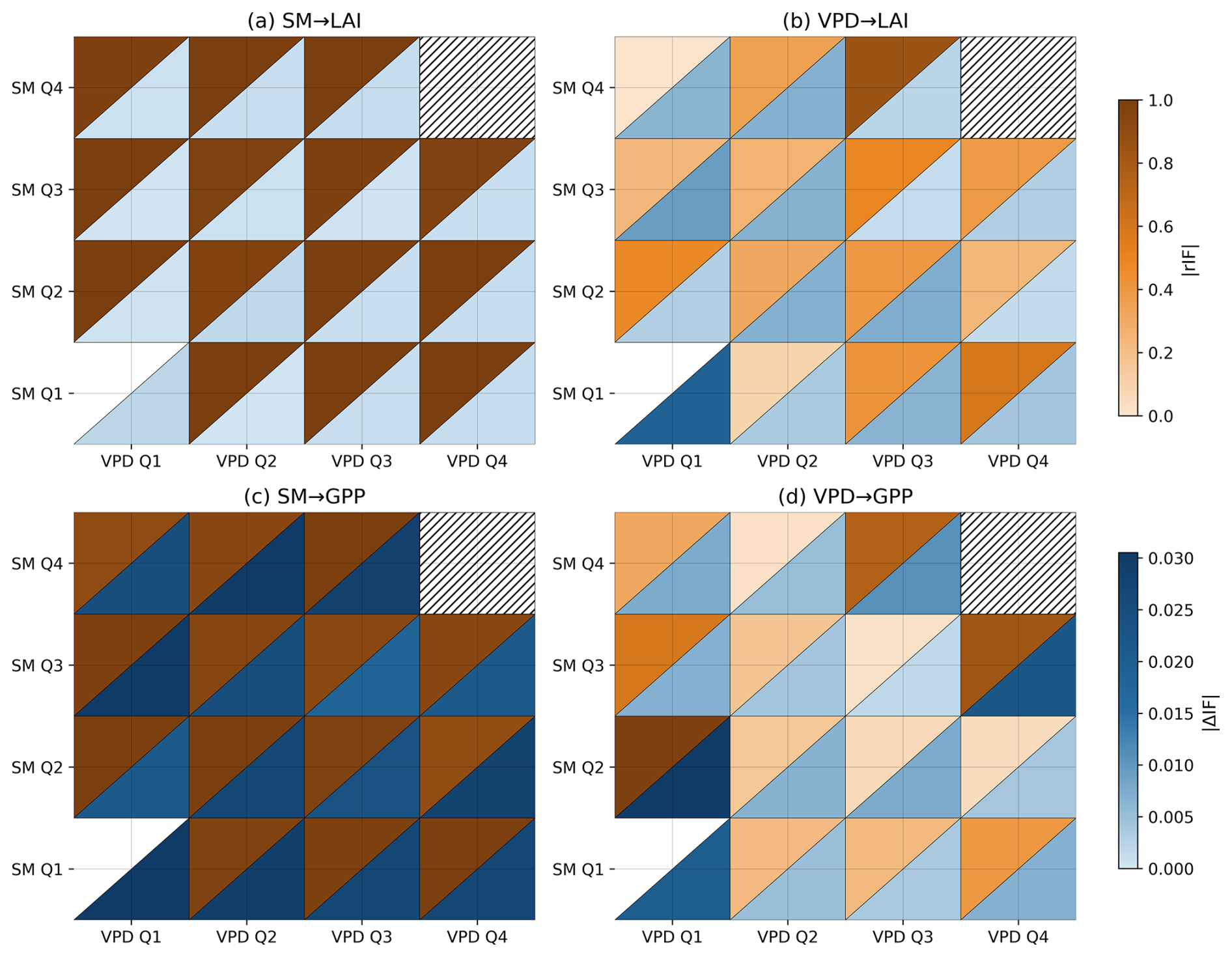
Figure 3 Differences (ΔIF) and correlations (rIF) between bivariate and multivariate Information Flow across SM and VPD quartiles (Q1–Q4) for Southeast China. (a) SM → LAI, (b) VPD → LAI, (c) SM → GPP, and (d) VPD → GPP. Each cell is divided into an upper triangle (|rIF|: magnitude of Pearson correlation between bivariate and multivariate IF) and a lower triangle (|ΔIF|: absolute difference between bivariate and multivariate IF). Colour intensities are scaled independently for each triangle using separable colormaps. Dark upper and lower triangles indicate similar temporal evolution (|rIF|) but large magnitude (|ΔIF|) differences between bivariate and multivariate IF. Light upper and lower triangles indicate small differences in both temporal behaviour and magnitude. Dark upper triangles with light lower triangles indicate similar temporal evolution with small magnitude differences, whereas light upper triangles with dark lower triangles indicate differences in both temporal behaviour and magnitude under conditioning. Blank upper triangles, such as that for SM(Q1)–VPD(Q1), indicate quartile combinations for which only two paired observations (n=2) were available; in these cases, |rIF| was not reported because Pearson correlation is not statistically informative with n=2, while the corresponding |ΔIF| value was retained. Cross-hatched cells indicate quartile combinations with no data. (SM = Soil Moisture, VPD = Vapor Pressure Deficit, LAI = Leaf Area Index, GPP= Gross Primary Productivity).

The VPD → LAI and VPD → GPP pathways (Fig. 3b, d) show wider variability in both |rIF| and |ΔIF|. Correlations range from weak to strong, and |ΔIF| spans small to large magnitudes across quartiles. This broad spread highlights the more nonlinear and state-dependent behavior of VPD-driven couplings. Figure S3a–c show the detailed |ΔIF| structure across regimes of water supply and atmospheric demand for all conditioning levels.

Overall, Fig. 3 shows that SM-based couplings (a, c) exhibit much greater uniformity than VPD-based couplings (b, d). The SM panels display consistent correlation strength and |ΔIF| patterns, whereas the VPD panels show substantial variation in both metrics. This suggests that VPD-driven interactions are more sensitive to environmental conditions and may require additional conditioning variables to achieve the stability seen in SM-driven couplings. Sensitivity tests using tercile- and quintile-based regime definitions yielded the same main qualitative conclusions and are provided in Fig. S4.

3.4 ANOVA of Regime-dependent Changes in Information Flow

This ANOVA framework (Appendix B) provides a variance-partitioning approach to quantify how variability in |ΔIF| is associated with individual hydroclimatic factors and their interactions.

3.4.1 Two-way ANOVA: moisture–demand control of |ΔIF|

Across all four pathways (SM → LAI, VPD → LAI, SM → GPP, VPD → GPP), the two-factor ANOVA partitions variability in |ΔIF| among the main effects of SM and VPD and their interaction (Fig. 4a). For the SM-driven pathways, the SM main effect dominates, whereas the VPD main effect contributes very little to |ΔIF| for these pathways.

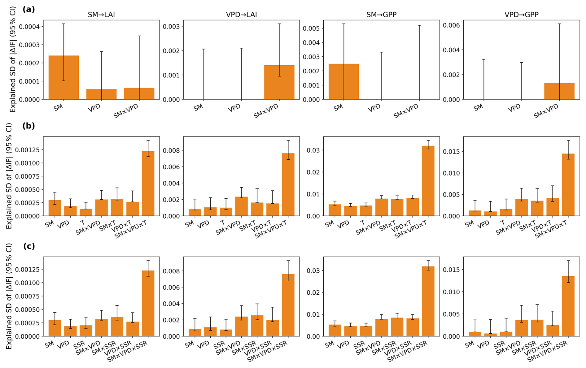
Figure 4 ANOVA results showing the explained standard deviation ($\sqrt{\mathrm{AEV}}$) of |ΔIF| for Southeast China. Columns represent the four pathways: SM → LAI, VPD → LAI, SM → GPP, and VPD → GPP. (a) Two-way ANOVA with factors SM and VPD. (b) Three-way ANOVA including SM, VPD, and T. (c) Three-way ANOVA including SM, VPD, and SSR. Bars show the explained SD for each factor or factor interaction; error bars indicate the 95 % confidence interval. (SM = Soil Moisture, VPD = Vapor Pressure Deficit, T= Temperature, SSR = Surface Solar Radiation). Note that the y-axis range differs in each panel to better see the different values.

For VPD-driven pathways, the SM × VPD interaction is the only dominant component, showing that the magnitude of the difference between the bivariate and multivariate IF estimates is more strongly associated with the combined moisture–demand regime rather than with either factor independently. The explained SD values are generally smaller for the LAI pathways and substantially larger for the GPP pathways.

3.4.2 Thermal modulation: SM × VPD × T structure

When temperature is included as a third factor, the SM×VPD×T interaction becomes the dominant component of the variance partitioning across all four pathways (Fig. 4b), whereas the main effects and two-way interactions contribute comparatively little. This dominance indicates a strongly non-additive relationship, in which variability in |ΔIF| is associated with the joint SM–VPD–T regimes rather than with consistent marginal associations of SM, VPD, or T individually.

3.4.3 Radiative modulation: SM × VPD × SSR structure

When SSR is included as a third factor, a similar pattern emerges, with the SM × VPD × SSR interaction becoming the dominant component of the variance partitioning across all four pathways (Fig. 4c), while the main effects and two-way interactions contribute comparatively little. This indicates that variability in |ΔIF| is primarily associated with the joint SM–VPD–SSR regimes rather than with consistent marginal associations of SM, VPD, or SSR individually. The corresponding variance fractions (ω2) for each pathway are shown in Fig. S5.

Altogether, the ANOVA results show that variability in |ΔIF| is strongly associated with interactions among the hydroclimatic factors, with the three-way interactions dominating when T or SSR is included. Although the explained SD values are substantially larger for the GPP pathways than for LAI (Fig. 4), the relative variance fractions (ω²) show broadly similar patterns across pathways (Fig. S5). The larger explained SD for GPP therefore largely reflects its larger overall |ΔIF| variability and does not imply a correspondingly greater relative contribution of the individual factors or interactions. Overall, these results indicate that variation in |ΔIF| depends strongly on the joint hydroclimatic regime, rather than on consistent effects of individual factors alone. Sensitivity analyses based on tercile- and quintile-based partitions show that the dominant higher-order interaction structure remains consistent (Fig. S6). Additional details on the ANOVA formulation and robustness considerations are provided in Appendix B.

3.5 Diagnosing the importance of Conditioners

Based on the results so far, we provide four indices that could be used to summarize how individual conditioners reshape the couplings by examining: (1) conditioner dominance index (CDI), (2) moderation gain (MG), (3) conditioning pressure (CP), and (4) convergence rate (CR). Here, we select the SM-driven couplings in Southeast China to simplify the demonstration. We thus highlight why SM → LAI and SM → GPP couplings behave so differently in terms of ΔIF. We note that for the purposes of this study, all the definitions provided here are strictly with respect to the LKIF.

CDI (Fig. 5a) quantifies the relative share of |ΔIF| attributable to each conditioner. VPD emerges as the dominant conditioner for both pathways, but especially for SM → GPP. For SM → LAI, VPD accounts for roughly two-thirds of the total |ΔIF|, while the remainder is distributed between T and SSR. This indicates that although VPD is the primary contributor, ΔIF for SM → LAI still reflects multiple environmental influences. In contrast, the SM → GPP pathway is almost entirely driven by VPD-related restructuring, with CDI close to 1 and only minor contributions from temperature and radiation. This concentration reveals that the discrepancy between bivariate and multivariate SM → GPP couplings is predominantly determined by VPD co-variation. This dominant VPD contribution is also consistent with the change in statistical significance described in Sect. 3.1, where adding VPD as a conditioner produces the largest increase in the occurrence of statistically significant SM → GPP IF (Table S1).

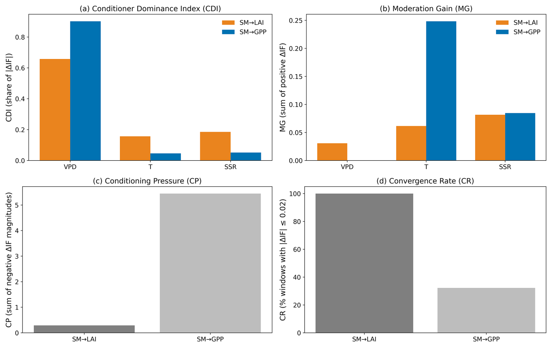
Figure 5 Importance of conditioning variables for |ΔIF| based on (a) Conditioner Dominance Index (CDI), (b) Moderation Gain (MG), (c) Conditioning Pressure (CP), and (d) Convergence Rate (CR), for the SM → LAI and SM → GPP couplings in Southeast China. In panel (c), CP is shown as the accumulated value across conditioners for each pathway.

MG (Fig. 5b) captures the sum of positive ΔIF values, representing decreases in IF across the conditioning sequence. For SM → LAI, MG is small for all conditioners, increasing slightly from VPD to T and reaching its largest value for SSR. This pattern indicates that T and SSR contribute larger decreases in IF than VPD, although these changes remain small for this pathway. In contrast, SM → GPP exhibits much larger MG dominated by temperature, with T producing a considerably larger moderation gain than VPD or SSR. This indicates that T contributes the largest decrease in IF relative to the preceding conditioning step, while SSR contributes a smaller decrease and VPD contributes little to the positive ΔIF component.

CP (Fig. 5c) measures the accumulated negative ΔIF and identifies cases in which conditioning increases the inferred IF. SM → LAI displays very low CP, indicating little increase in IF after conditioning. SM → GPP, however, shows much larger accumulated CP, indicating that conditioning produces a larger increase in the inferred IF. This is consistent with Fig. 1c, where the bivariate SM → GPP estimate is generally lower than the corresponding conditioned estimates. This confirms that the bivariate representation of SM → GPP can markedly understate the inferred IF relative to the conditioned coupling.

CR (Fig. 5d) quantifies the percentage of time windows in which |ΔIF| remains below a small threshold and thus reflects how often the bivariate and fully conditioned estimates are close to each other. SM → LAI has a CR near 100 %, indicating that the bivariate and multivariate IF estimates almost always agree and that conditioning on additional variables rarely leads to substantial changes in the inferred IF. In contrast, SM → GPP shows a much lower CR, meaning that the bivariate estimate frequently diverges from the multivariate one, and conditioning is essential for an accurate causal representation. Although CR varies with ϵ_abs, the main interpretation remains unchanged, with SM → LAI showing consistently high convergence and SM → GPP remaining more threshold-sensitive and less convergent overall (Fig. S7).

A permutation test of the sequential decomposition showed that CDI and MG are sensitive to the order in which the conditioners are introduced (Fig. S8). Despite this order dependence, the permutation-averaged CDI retained VPD as the dominant conditioner for both SM–LAI and SM–GPP, whereas MG exhibited pronounced order-related variability, most notably for T in the SM–GPP pathway (Fig.  S9 in the Supplement). For SM → LAI, the relative ranking of VPD and SSR varies across permutations, suggesting that conditioner dominance for this pathway is order-sensitive. For SM → GPP, VPD remains a leading and often dominant contributor across the tested permutations, although the exact CDI and MG values vary with order. In contrast, CR remained unchanged across permutations, and the aggregated CP also remained unchanged in the present application. The sensitivity and robustness of these indices to noise and record length are further evaluated in the Supplement (Table S3; Fig. S10).

Figure 5 demonstrates a clear structural–functional divide in vegetation–climate coupling. The SM → LAI pathway shows weak sensitivity to the selected additional variables: conditioning effects are small, conditioning pressure is negligible, and bivariate and multivariate IF show consistent agreement. In contrast, the SM → GPP pathway is strongly conditioner-dependent. VPD remains a leading contributor to its ΔIF structure across permutations, while temperature and radiation contribute to the divergence, and SM → GPP exhibits much larger accumulated CP than SM → LAI. These findings show that some vegetation couplings (e.g., SM → LAI) are robust to the selected conditioners, whereas other pathways, such as SM → GPP, depend critically on accounting for conditioner effects to correctly characterize their causal behavior. The corresponding SM–VPD quartile-specific results are shown in Fig. S11.

4 Discussion

Understanding cause–effect relationships in land–atmosphere systems remains challenging because interacting drivers and shared variability obscure direct and indirect influences. Several causal methods have been used to identify directional relationships, although they differ in how they handle conditioning variables. GC infers lagged directional dependence through autoregressive predictability and can be extended to conditional or multivariate forms, yet its ability to control conditioning depends on explicitly including additional variables and can weaken as dimensionality increases (Papagiannopoulou et al., 2017; Krich et al., 2020). Information-theoretic approaches, such as transfer entropy and process-network frameworks, can capture nonlinear dependencies and feedback structures, but their multivariate application is limited by data demands and the curse of dimensionality (Ruddell and Kumar, 2009; Krich et al., 2020). PCMCI addresses this more explicitly by using conditional independence tests to remove indirect pathways and the influence of observed common drivers, although it still relies on assumptions such as causal sufficiency and stationarity, leaving potential sensitivity to hidden or time-varying confounders (Krich et al., 2020; Docquier et al., 2024). LKIF provides a physically grounded asymmetric measure of directed influence and has been applied in land–atmosphere studies of SM impacts on temperature and precipitation (Liu and Pu, 2019; Hagan et al., 2019; Takaya et al., 2025; Sun et al., 2025), with recent multivariate extensions allowing explicit conditioning on additional variables (Liang, 2021; Zhou et al., 2024). However, attempts to understand how conditioners may influence its causal structures are still limited. Here, using the differences between bivariate and multivariate LKIF (ΔIF), we explore the impact of conditioners on its causal estimations. We find that this difference is physically informative, such that the divergence between the two identifies when apparent driver–response relationships are robust to conditioning and when they depend on additional variables.

In addition to these methodological differences, the temporal resolution and lag structure used in LKIF are important for interpreting the estimated information flow. In the present study, the temporal derivative of the target variable for each information-flow direction is approximated by first-order differencing over the monthly sampling interval (dt = 1 month). This monthly temporal step enters the LKIF estimation through the discrete approximation of the target-variable tendency but differs from an explicit lagged analysis in which the source variable is shifted relative to the target. Previous applications have shown that LKIF estimates can vary with both lag structure and temporal resolution. Introducing lagged variables can reveal causal relationships that are weak or absent in contemporaneous analyses, while temporal averaging and sampling frequency can modify the magnitude and structure of the estimated information flow (Docquier et al., 2023, 2024). Our results should therefore be interpreted within the monthly temporal framework used here. A systematic assessment of different temporal resolutions and lag structures therefore represents an important direction for future work.

Building on this framework, ΔIF provides a direct measure of how strongly conditioning alters the inferred pathway. In the present application, ΔIF is not uniformly large or small, but varies systematically across couplings and environmental regimes. The influence of SM on LAI shows persistently low ΔIF and strong agreement between bivariate and multivariate estimates, whereas the influence of SM on GPP and the VPD-driven pathways exhibits much larger and more variable divergence, particularly under dry, high VPD, hot, and high radiation conditions. This indicates that the role of conditioning is state-dependent, such that under some conditions, the bivariate estimate captures the dominant pathway, whereas under others, the inferred relationship changes substantially once additional variables are included. Such state dependence is particularly relevant in land–atmosphere systems, where interactions among moisture, energy, and atmospheric demand intensify under compound stress.

This state dependence is particularly evident for the SM → GPP coupling in Southeast China, where conditioning on VPD substantially increases the temporal persistence of statistically significant IF compared to the bivariate form (Sect. 3.1; Table S1). This behavior is consistent with the joint regulation of vegetation productivity by soil water supply and atmospheric demand; low SM restricts plant water supply, whereas high VPD increases atmospheric water demand and can induce stomatal closure, thereby reducing photosynthetic carbon uptake (Novick et al., 2016; Yuan et al., 2019). Because SM and VPD covary through land–atmosphere interactions, distinguishing their individual influences on GPP in a bivariate analysis can be challenging. In our analysis, the bivariate SM → GPP pathway is significant primarily around the 2011 drought (Sun and Yang, 2012). Under such dry conditions, increasing soil water limitation can constrain stomatal conductance and photosynthetic carbon uptake, thereby increasing the sensitivity of GPP to SM (Fu et al., 2022). This may help explain why the SM → GPP relationship becomes detectable even without conditioning. Conversely, the VPD-conditioned coupling remains significant over a much larger fraction of the record. This contrast is consistent with partial masking of the SM-related contribution by shared SM–VPD variability in the bivariate representation, whereas accounting for VPD allows the SM-related contribution to be detected more consistently. Temperature and SSR may further modulate this separation through their influence on atmospheric demand and photosynthetic energy availability, consistent with the higher-order hydroclimatic interactions identified in Sect. 3.4. The Amazon Basin shows the opposite significance response (Sect. 3.1; Table S2), indicating that the effect of conditioning on the statistical significance of SM → GPP is region-dependent and can operate in either direction.

The four proposed indices (Sect. 3.5; CDI, MG, CP, and CR) are important because they make this divergence diagnostically interpretable and comparable across pathways. ΔIF indicates whether conditioning matters, but not whether its effect is pathway-specific, concentrated under particular environmental conditions, or associated with convergence between simpler and more complete formulations. The indices provide a compact framework for resolving these dimensions systematically. They allow the analysis to move beyond detecting divergence to identifying when bivariate and conditioned representations are very similar, when additional variables materially alter inference, and where causal refinement is most needed. In this way, they strengthen the methodological contribution of the LKIF framework by making pathway sensitivity to conditioning explicit and comparable across couplings.

These findings also point to a broader application of the framework in model evaluation. Because the framework identifies when inferred pathways are stable and when they are strongly conditioning dependent, it offers a means to assess how land–atmosphere interactions are represented in Earth system models. Applied to climate model simulations, including Coupled Model Intercomparison Project Phase 6 (CMIP6), these diagnostics could test whether models reproduce not only the magnitude of vegetation–climate coupling, but also its sensitivity to co-varying drivers and its reorganization under compound stress. This would provide a more process-based benchmark than evaluations based only on mean states or correlations.

Several limitations should be considered when interpreting these results. First, the analysis is based on a time-varying linear formulation of the LKIF framework, which may not fully capture nonlinear feedbacks and state-dependent shifts under extreme conditions. Second, the inferred causal structure depends on the selected conditioning variables. Although SM, VPD, T, and SSR represent dominant environmental controls, omitted variables may still influence the estimated relationships. Third, the proposed indices depend on the conditioning design and should therefore be interpreted as diagnostic summaries of pathway sensitivity, rather than as universal causal measures. Fourth, uncertainties in observational and reanalysis datasets, together with the aggregation to monthly temporal scales, may affect both the magnitude and variability of the estimated information flows. Finally, the real-world application is limited to two humid forest biomes and therefore does not capture the broader range of hydroclimatic variability across global ecosystems. Vegetation responses in drylands are more directly constrained by SM deficits, whereas high-latitude systems are more strongly influenced by temperature and radiation limitations (D'Orangeville et al., 2018; Liu et al., 2020; Xie et al., 2024). These differences may alter both the magnitude and structure of LKIF, as well as the relative importance of conditioners. Extending the framework across a broader range of biomes, incorporating additional conditioning variables, and exploring nonlinear extensions of the method, therefore, represent important directions for future work.

5 Conclusion

This study investigated when and why conditioners may alter information flow pathways. We achieved this by analyzing divergence between the bivariate and multivariate formulations of Liang–Kleeman Information Flow (LKIF), and how these differences reflect the contribution of the conditioners to an application in land–atmosphere interactions. A synthetic validation (Appendix A) showed that LKIF preserves directional fidelity under hidden confounding, though differences between bivariate and multivariate estimates still occur.

A real-world application (Sect. 3) revealed that the impacts of conditioners on causal structures vary across time and space, demonstrating that spatial and temporal averaging could mask the relevance of conditioners. In our study, SM → LAI, representing vegetation structure, showed consistently high similarity between the bivariate and multivariate estimates across locations and time, with minimal conditioner influence and a high convergence rate. In contrast, SM → GPP, representing vegetation function, exhibited strong conditioner dependence, substantial divergence, and marked temporal variability. These differences were particularly pronounced during periods of compound stress, when atmospheric demand, temperature, or radiation jointly altered the inferred causal pathway. VPD emerged as the dominant conditioner shaping ΔIF for SM → GPP, while temperature showed the largest decrease in IF when included as a conditioner. Together, these patterns demonstrate that conditioning variables produce much larger modifications in the functional pathways than in the structural ones.

We also found that the physical states of the driver variables further controlled the degree of divergence. SM-driven couplings showed stable behavior across supply–demand states, whereas VPD-driven couplings displayed wide variability in both rIF and ΔIF. ANOVA confirmed that the largest departures occurred under combinations of dryness, high VPD, and elevated T/SSR conditions known to intensify plant stress. These state-dependent effects explain why conditioners appear intermittently, because their influence strengthens only when climatic conditions amplify dependencies among drivers. Importantly, similarity between bivariate and conditioned estimates should not be interpreted as evidence of causal sufficiency, because relevant conditioner effects may offset one another or important variables may remain unobserved. In contrast, under more complex or compound-stress conditions, conditioning can substantially modify the inferred coupling, including its magnitude and statistical significance. These conclusions are drawn from two humid forest regions, Southeast China and the Amazon Basin, and should therefore not be generalized across all biomes. In drier or colder ecosystems, the relative importance of conditioners may differ because vegetation is regulated by different dominant constraints.

While this work does not include all potential conditioners, the selected variables represent dominant environmental controls and yield physically interpretable causal signals. Nevertheless, the inferred pathways remain conditional on the variables included, the linear formulation used here, and the sampling characteristics of the observations. In parallel with observation-based causal analysis, future work should therefore use targeted process-based numerical experiments to evaluate the identified pathways and conditioning effects under controlled changes in omitted processes, nonlinear interactions, and sampling characteristics. Such complementary modelling analyses would help assess the physical robustness of the inferred conditioning effects. To better capture complex feedbacks that arise during extreme events, nonlinear extensions of the LKIF framework (Pires et al., 2024; Vannitsem et al., 2025) should also be explored. The present analysis does not evaluate lag-specific driver-response relationships. Given that land–atmosphere interactions may exhibit memory over weeks to months, future work should investigate how the inferred information flows and the influence of conditioning variables vary across different temporal lags.

Our findings provide conceptual and practical frameworks for deciding when conditioning is necessary and highlight the importance of considering conditioners in future applications of Information Flow to land–atmosphere systems. Furthermore, this framework may also support feature selection in machine learning by identifying drivers with an inferred directional causal influence and revealing when inferred relationships are strongly affected by conditioning, an application that remains to be explored.

Appendix A: Synthetic data experiments

We begin by demonstrating how hidden confounders influence information-flow estimation through a controlled synthetic experiment. The goal is to assess whether LKIF can still recover a faithful causal structure when parts of the underlying system are unobserved, a situation frequently encountered in Earth-system applications. The experiment uses a five-dimensional, linear, stable Vector Autoregressive (VAR1) process defined as (Eq. A1);

$$\begin{array}{}\text{(A1)}& {\mathit{x}}_t=\mathbf{A}{\mathit{x}}_{t-\mathrm{1}}+{\mathit{ϵ}}_t,{\mathit{ϵ}}_t\sim \mathcal{N}(\mathrm{0},\mathbf{\Sigma }),\end{array}$$

where ${\mathit{x}}_t={\left(x_{\mathrm{1},t},x_{\mathrm{2},t},x_{\mathrm{3},t},x_{\mathrm{4},t},x_{\mathrm{5},t}\right)}^{\mathrm{\top }}$ are the five different time series and $\mathbf{\Sigma }=\mathrm{diag}\left(b_{\mathrm{1}}^{\mathrm{2}},b_{\mathrm{2}}^{\mathrm{2}},b_{\mathrm{3}}^{\mathrm{2}},b_{\mathrm{4}}^{\mathrm{2}},b_{\mathrm{5}}^{\mathrm{2}}\right)$, with b_i being the stochastic perturbation amplitudes The coefficient matrix A is (Eq. A2);

$$\begin{array}{}\text{(A2)}& \mathbf{A}=\left(\begin{array}{ccccc}\mathit{\varphi }& c_{\mathrm{21}}& c_{\mathrm{31}}& \mathit{\gamma }& \mathrm{0}\\ c_{\mathrm{12}}& \mathit{\varphi }& c_{\mathrm{32}}& \mathit{\gamma }& \mathrm{0}\\ \mathrm{0}& \mathrm{0}& \mathit{\varphi }& \mathrm{0}& \mathrm{0}\\ \mathrm{0}& \mathrm{0}& \mathrm{0}& \mathit{\varphi }& \mathit{\eta }\\ \mathrm{0}& \mathrm{0}& \mathrm{0}& \mathrm{0}& \mathit{\varphi }\end{array}\right)\end{array}$$

encodes all causal interactions, where $\mathit{\varphi }=\mathrm{0.25},c_{\mathrm{21}}=\mathrm{0.05},c_{\mathrm{31}}=\mathrm{0.55},c_{\mathrm{32}}=\mathrm{0.12},c_{\mathrm{12}}=\mathrm{0.45}$, $\mathit{\eta }=\mathrm{0.70},$ and γ is a parameter that varies between 0 and 0.8. The innovation scales are $\left(b_{\mathrm{1}},b_{\mathrm{2}},b_{\mathrm{3}},b_{\mathrm{4}},b_{\mathrm{5}}\right)=\left(\mathrm{0.6},\mathrm{0.5},\mathrm{0.5},\mathrm{0.6},\mathrm{0.6}\right)$. Expanding (VAR1) by rows gives (Eq. A3);

$$\begin{array}{}\text{(A3)}& \begin{array}{l}{x}_{\mathrm{1},t}=\mathit{\varphi }{x}_{\mathrm{1},t-\mathrm{1}}+c_{\mathrm{21}}{x}_{\mathrm{2},t-\mathrm{1}}+c_{\mathrm{31}}{x}_{\mathrm{3},t-\mathrm{1}}+\mathit{\gamma }{x}_{\mathrm{4},t-\mathrm{1}}+{\mathit{ϵ}}_{\mathrm{1},t},\\ x_{\mathrm{2},t}=\mathit{\varphi }{x}_{\mathrm{2},t-\mathrm{1}}+c_{\mathrm{12}}{x}_{\mathrm{1},t-\mathrm{1}}+c_{\mathrm{32}}{x}_{\mathrm{3},t-\mathrm{1}}+\mathit{\gamma }{x}_{\mathrm{4},t-\mathrm{1}}+{\mathit{ϵ}}_{\mathrm{2},t}\\ x_{\mathrm{3},t}=\mathit{\varphi }{x}_{\mathrm{3},t-\mathrm{1}}+{\mathit{ϵ}}_{\mathrm{3},t}\\ x_{\mathrm{4},t}=\mathit{\varphi }{x}_{\mathrm{4},t-\mathrm{1}}+\mathit{\eta }{x}_{\mathrm{5},t-\mathrm{1}}+{\mathit{ϵ}}_{\mathrm{4},t}\\ x_{\mathrm{5},t}=\mathit{\varphi }{x}_{\mathrm{5},t-\mathrm{1}}+{\mathit{ϵ}}_{\mathrm{5},t}.\end{array}\end{array}$$

This structure separates the system into observable and hidden components. Only $x_{\mathrm{1}},x_{\mathrm{2}},x_{\mathrm{3}}$ are assumed observable and are used for the IF estimation, whereas x₄ and x₅ act as hidden confounders. The causal design includes a bidirectional interaction between x₁ and x₂, unidirectional influences x₃→x₁ and x₃→x₂, and a hidden driver x₄ that drives both x₁ and x₂. A deeper, nested confounder x₅ drives x₄ (Fig. A1a). This nested confounding structure aims to mimic realistic Earth-system conditions where unobserved processes can influence, or even generate, additional confounders. To examine how confounding strength affects IF estimation, we vary the parameter $\mathit{\gamma }\in \mathit{\{}\mathrm{0.0},\mathrm{0.1},\mathrm{\dots },\mathrm{0.8}\mathit{\}}$, which controls the influence of the hidden confounder x₄ on the observable variables x₁ and x₂. For each γ, multiple independent realizations of length N=3000 are generated.

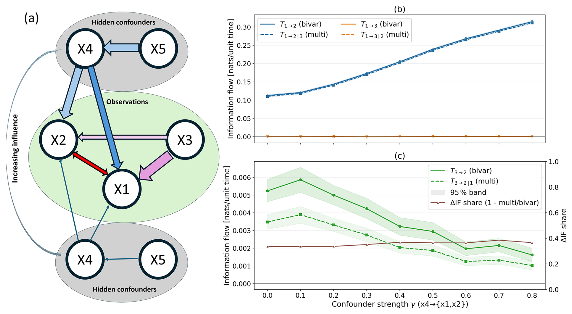
Figure A1 Toy-model experiment illustrating the effect of hidden confounders on Liang–Kleeman Information Flow (LKIF). (a) Causal graph for a five-variable system with three observed variables ($x_{\mathrm{1}},x_{\mathrm{2}},x_{\mathrm{3}}$) and two hidden confounders (x₄, x₅). Directed arrows show the true causal pathways; blue arrows represent pathways originating from hidden confounders, the red arrow denotes the bidirectional coupling between x₁ and x₂, and the pink arrows denote the causality of x₃→x₁ and x₃→x₂. Estimated bivariate (solid lines) and multivariate (dashed lines) IF for (b) x₁→x₂ and x₁→x₃ and (c) x₃→x₂ under increasing confounder strength γ, with the brown line showing the normalized difference (right y-axis). The shaded band shows the 95 % confidence intervals.

For every γ value, we compute the bivariate information flows $T_{\mathrm{1}\to \mathrm{2}}^{\left(\mathrm{bi}\right)}$ and  $T_{\mathrm{1}\to \mathrm{3}}^{\left(\mathrm{bi}\right)}$ each using only the two variables involved, and the multivariate (conditioned) information flows $T_{\mathrm{1}\to \mathrm{2}|\mathrm{3}}^{\left(\mathrm{mv}\right)}$ and $T_{\mathrm{1}\to \mathrm{3}|\mathrm{2}}^{\left(\mathrm{mv}\right)}$ where one additional observed variable is included as a conditioning variable. To evaluate how conditioning alters the estimated causal strength, we compute the differential information flows using Eq. (3) as (Eqs. A4–A5);

$$\begin{array}{}\text{(A4)}& {\displaystyle }\mathrm{\Delta }{\mathrm{IF}}_{\mathrm{1}\to \mathrm{2}}=T_{\mathrm{1}\to \mathrm{2}}^{\left(\mathrm{bi}\right)}-T_{\mathrm{1}\to \mathrm{2}|\mathrm{3}}^{\left(\mathrm{mv}\right)}\text{(A5)}& {\displaystyle }\mathrm{\Delta }{\mathrm{IF}}_{\mathrm{1}\to \mathrm{3}}=T_{\mathrm{1}\to \mathrm{3}}^{\left(\mathrm{bi}\right)}-T_{\mathrm{1}\to \mathrm{3}|\mathrm{2}}^{\left(\mathrm{mv}\right)}\end{array}$$

Across 80 realizations, we compute bootstrap mean bands for each γ using B=1000 resamples, and percentile ribbons at the 95 % range. A significance mask marks ΔIF (or T) as significant when the bootstrap band excludes zero. These estimations are repeated for x₃→x₂, as well to also quantify the influence of the mediator x₁.

The results are summarized in Fig. A1, which illustrates the causal structure and clearly distinguishes observed and hidden components. The green region highlights the observable variables ($x_{\mathrm{1}},x_{\mathrm{2}},x_{\mathrm{3}}$) used to compute IF. The grey regions contain the hidden confounders x₄ and x₅, which influence the system but are deliberately excluded from the estimation. The hidden confounder x₄ injects shared variability into both x₁ and x₂, while the additional variable x₅ introduces a deeper causal layer, creating a confounder-of-a-confounder structure. As γ increases, the influence of the hidden confounder x₄ on the observed variables becomes stronger, amplifying the confounding pressure that cannot be removed through conditioning on observed variables alone. This ensures that the observable system is subjected to increasing and unresolvable confounding, allowing the experiment to test whether IF remains reliable under such challenging conditions.

Figure A1b shows that the IF from x₁→x₃ remains essentially zero across all γ values. This behavior is fully consistent with the underlying system, which contains no direct causal link from x₁ to x₃. Both the bivariate and multivariate IF estimates demonstrate that the presence of hidden confounders does not induce spurious causal inference in these couplings. In contrast, the causal pathway x₁→x₂ is consistently detected, although it strengthens as γ increases. The IF values for this pathway show a rise with increasing hidden confounder strength, reflecting the fact that x₄ amplifies the coupling between x₁ and x₂ since x₄ increases the feedback between x₁ and x₂. Importantly, the bivariate and multivariate IF curves for x₁→x₂ remain nearly indistinguishable throughout the entire γ range, indicating that conditioning on x₃ provides only a negligible adjustment for this pathway. In contrast, for x₃→x₂, conditioning on x₁ changes the magnitude of the estimated IF, while the inferred causal direction remains unchanged (Fig. A1c). These results show that the response to conditioning differs between the pathways considered in the synthetic experiment. The present synthetic configuration, however, does not exhibit conditioning-induced transitions in statistical significance between the bivariate and multivariate estimates. Because conditioning can affect not only IF magnitude but also its statistical significance, we performed an additional 3-variable controlled experiment specifically designed to examine this transition. With a fixed direct pathway, progressively strengthening an opposing common-driver pathway causes the bivariate estimate to become statistically non-significant, while the corresponding conditioned estimate remains significant (Sect. S1; Fig. S13).

Overall, this theoretical experiment demonstrates that LKIF retains directional fidelity under increasing and nested hidden confounding. True causal connections, such as x₁→x₂, are consistently recovered, while nonexistent connections remain near zero. This result is consistent with the findings in Vannitsem et al (2024).

The reduction of IF after conditioning in Fig. A1c reflects the particular pathway configuration prescribed in this synthetic experiment and is not a general requirement of conditional information flow. To examine the reverse case, we repeated the experiment with the sign of the x₁→x₂ coefficient reversed from C₁₂=0.45 to $C_{\mathrm{12}}=-\mathrm{0.45}$, while retaining all other model parameters. This makes the direct x₃→x₂ pathway and the indirect pathway through x₁ act in opposite directions. Under this configuration, the conditioned IF $x_{\mathrm{3}}\to x_{\mathrm{2}|\mathrm{1}}$ consistently exceeds the corresponding bivariate x₃→x₂ estimate, yielding negative ΔIF across the full range of confounder strengths (Fig. S12). Thus, conditioning can either reduce or enhance the estimated IF depending on the structure and signs of the interacting pathways.

The present synthetic experiment is intended as a controlled assessment of LKIF under the specific hidden-confounding structure considered here and does not constitute a systematic benchmark across all possible causal structures. In particular, configurations involving hidden mediators, colliders, observable forks, joint conditioning structures, or parallel pathways with compensating effects are not systematically evaluated. This distinction is important for interpreting |ΔIF|. A small |ΔIF| indicates that the bivariate and multivariate estimates are very similar for the specified conditioning set but does not establish causal sufficiency. For example, different pathways may make individually important contributions with opposing signs and similar magnitudes, resulting in a small overall difference. Similarly, when a relevant mediator is unobserved, the present experiment does not establish that its contribution can be uniquely separated within the observed subsystem. A systematic assessment of LKIF under these different causal structures represents an important direction for future work.

Appendix B: ANalysis Of Variance (ANOVA)

ANalysis Of Variance (ANOVA) was applied to the |ΔIF| values to quantify how their variability is structured across different hydroclimatic regimes. Monthly SM, VPD, T, and SSR were each partitioned into quartiles (Q1–Q4) using empirical quantiles. These quartile categories were then treated as factors in the ANOVA, which reports variance components across quartiles rather than individual quartile means. Three experimental designs were used:

1. a two-way ANOVA: SMq×VPDq.

2. a three-way thermal ANOVA: $\mathrm{SMq}\times \mathrm{VPDq}\times Tq$.

3. a three-way radiative ANOVA: $\mathrm{SMq}\times \mathrm{VPDq}\times \mathrm{SSR}$.

These designs represent water supply (SM), atmospheric demand (VPD), and energy constraint (Temperature or SSR) regimes.

For each design, ANOVA decomposed the variability in |ΔIF| according to the general multi-factor model (Eq. B1),

$$\begin{array}{}\text{(B1)}& \begin{array}{rl}Y& =\mathit{\mu }+\mathit{\alpha }i+\mathit{\beta }j+\mathit{\gamma }k+\mathit{\delta }l+\left(\mathit{\alpha }\mathit{\beta }\right)ij+\left(\mathit{\alpha }\mathit{\gamma }\right)ik\\ & +\left(\mathit{\beta }\mathit{\gamma }\right)jk+\left(\mathit{\alpha }\mathit{\beta }\mathit{\gamma }\right)ijk+\mathrm{\cdots }+\mathit{ϵ}ijkl,\end{array}\end{array}$$

In this model, Y denotes the |ΔIF| values for each combination of SM, VPD, and T/SSR quartiles. The term μ is the grand mean, while αi, βj, γk and δl represent the main effects of SM, VPD, T, and SSR quartiles. The interaction terms αβij, αγik, βγjk, and (αβγ)ijk capture how combinations of these factors jointly modify |ΔIF| beyond their individual effects. The residual ϵijkl accounts for unexplained variability.

In Eq. (B2), the total variability was partitioned into sums of squares using

$$\begin{array}{}\text{(B2)}& {\mathrm{SS}}_{\mathrm{Total}}={\sum }_{t=\mathrm{1}}^N{\left(yt-\stackrel{\mathrm{‾}}{y}\right)}^{\mathrm{2}}\end{array}$$

Here, yt represents each |ΔIF| value, $\stackrel{\mathrm{‾}}{y}$ is the overall mean across all |ΔIF| values, and SS_Total measures the total variability in |ΔIF| before attributing it to any factor or interaction.

In Eq. (B3),

$$\begin{array}{}\text{(B3)}& {\mathrm{SS}}_X={\sum }_{i}ni(\stackrel{\mathrm{‾}}{yi}-\stackrel{\mathrm{‾}}{y}{)}^{\mathrm{2}}\end{array}$$

SS_X quantifies the amount of |ΔIF| variability explained by a specific factor X (SM, VPD, temperature, SSR). Here, $\stackrel{\mathrm{‾}}{yi}$ is the mean |ΔIF| for level i of factor X, ni is the number of observations in that level, and $\stackrel{\mathrm{‾}}{y}$ is the overall mean. The same structure applies to interaction terms (e.g., SS_SM×VPD), where the means $\stackrel{\mathrm{‾}}{yi}j$ correspond to pairs (or triples) of factor levels.

The residual variability is (Eq. B4),

$$\begin{array}{}\text{(B4)}& {\mathrm{SS}}_{\mathrm{Error}}={\mathrm{SS}}_{\mathrm{Total}}-{\sum }_X{\mathrm{SS}}_X\end{array}$$

represents the portion of |ΔIF| not accounted for by any main factor or interaction term.

To characterize the strength of each regime effect, the bias-corrected omega-squared statistic was used (Eq. B5),

$$\begin{array}{}\text{(B5)}& {\mathit{\omega }}_{X=}^{\mathrm{2}}{\displaystyle \frac{{\mathrm{SS}}_X-{\mathrm{df}}_X{\mathrm{MS}}_{\mathrm{Error}}}{{\mathrm{SS}}_{\mathrm{Total}}+{\mathrm{MS}}_{\mathrm{Error}}}}\end{array}$$

This equation defines omega-squared for factor X, which measures the proportion of the variance in |ΔIF| that is attributable to that factor after correcting for bias. SS_X is the sum of squares explained by factor X, and df_X is the degrees of freedom associated with it. MS_Error is the mean square of the residual error and equal to ${\mathrm{MS}}_{\mathrm{Error}}={\mathrm{SS}}_{\mathrm{Error}}/{\mathrm{df}}_{\mathrm{Error}}$. SS_Total is the total sum of squares of |ΔIF|.

Omega-squared provides a bias-corrected estimate of the fraction of total |ΔIF| variability explained by factor X. Larger values of ${\mathit{\omega }}_X^{\mathrm{2}}$ indicate that the environmental regime represented by X plays a stronger role in shaping |ΔIF|.

The corresponding physically interpretable magnitude was given by the explained standard deviation (Eq. B6),

$$\begin{array}{}\text{(B6)}& {\mathrm{SD}}_x={\mathit{\sigma }}_{\mathit{\gamma }}\sqrt{\mathit{\omega }{{}_x}^{\mathrm{2}}}\end{array}$$

expressed in the same units as |ΔIF|, where σ_γ is the standard deviation of |ΔIF| and $\mathit{\omega }{{}_x}^{\mathrm{2}}$ is the variance explained by factor X. Bootstrap resampling within each SM × VPD (or SM × VPD × T/SM × VPD × SSR) regime provided 95 % confidence intervals for both ω² and SD.

While ANOVA provides a useful framework for partitioning variability in |ΔIF| across hydroclimatic regimes, it is important to note that its classical assumptions may not be fully satisfied in this context. The |ΔIF| values are derived from monthly time series and may therefore retain temporal dependence, meaning that observations are not strictly independent. In addition, the use of quantile-based regime definitions can lead to unequal variance across bins (heteroscedasticity), particularly in extreme or sparsely populated regime combinations. In this study, ANOVA is therefore interpreted primarily as a variance-partitioning and effect-size diagnostic, rather than as a strict inferential test under ideal assumptions. To assess robustness, we complement the analysis with alternative regime definitions (terciles and quintiles; Fig. S6). The main qualitative conclusions, particularly the dominant role of higher-order interactions, remain consistent across these tests, although some weaker two-way effects show greater sensitivity to binning choice.