Can we define climate by means of an ensemble? A tale of time scales of convergence

It is not really questioned today that climate can be described in theory by an ensemble of trajectories differing in their initial conditions, which is then translated to numerical ensembles in climate models. It is also widely accepted that any evolution observed within a few decades after initialization is not yet relevant to climate. Evolution at a later stage, instead, is then used to characterize climate and its change, under the implicit assumption that slower processes do not considerably contribute to differences between ensemble members, allowing internal variability of climate to be identified with these differences. However, a careful justification for this practice is as yet lacking. In particular, a definition of climate in support of this practice is outstanding, including the identification of the kind of time scales at play through providing an argumentation for their relevance. Our study aims at filling this gap. After pointing out that the most important criterion for a definition of climate is the uniqueness of the probability measure on which the definition relies, we first recall the naive proposal to represent such a probability measure by the distribution of ensemble members that has, loosely speaking, converged to the natural probability measure of the so-called snapshot or pullback attractor of the dynamics. We then consider the time scales of convergence and refine the proposal by taking a probability measure that is conditional on the (possibly time-evolving) state of modes characterized by convergence time scales longer than the horizon of a particular study. We design an ensemble simulation initialization scheme for studying convergence time scales and uniqueness of ensembles in Earth system models.

1 Motivation

In roughly the past two decades, 𝒪(10)–𝒪(100)-member initial-condition ensemble simulations have become increasingly popular in single state-of-the-art Earth system models (e.g., Kay et al., 2015; Maher et al., 2019; Rodgers et al., 2021), and this trend is expected to continue (e.g., Mankin et al., 2020). The aim of these projects is the identification of forced responses and the exploration of the internal variability of climate under explicit time dependence (which the word “forcing” will refer to throughout this article). The motivation for this kind of investigation is based on the naive recognition (e.g., Deser et al., 2020, and references therein) that the Earth system (and models thereof) permits a plethora of equally plausible states (e.g., weather configurations) at any time instant, even if this instant occurs during an active forcing scenario¹. From this point of view, the ensembles in question are intended to represent that set of states of the system; for this purpose, their different members have been generated with the same forcing scenario but stem from different initial conditions. Climatological mean values are then identified with the ensemble mean, and it is more and more widespread to describe the internal variability of climate by further statistical quantifiers evaluated with respect to the ensemble. In turn, the time evolution of all these statistical quantifiers (including but not restricted to the mean) is usually identified with their forced response.

One assumption behind these interpretations is that climate, as a statistical description of weather (IPCC, 2021), is represented by the distribution of the ensemble members; if one likes, this may be regarded as a definition of climate (at least in the given models; and this definition is then certainly more useful than those relying on temporal averaging). However, no careful justification for this assumption has been provided to date. In fact, not even a framework or construction has been identified that would allow for such a justification from “first principles” (ab initio). The aim of the present article is to identify one; i.e., not a justification, but a way of analysing the system, an already existing mathematical description of probability measures associated with the system, that makes justification qualitatively well-posed.

We emphasize that we are looking for a kind of ab initio description. While no model can resolve all of the processes relevant to climate, the reasonably good performance of global climate or Earth system models in describing the real world supports the view that the climate system or the Earth system is basically a nonautonomous dissipative deterministic dynamical system; genuine stochasticity may enter on the smallest spatial and temporal scales only and is thus not directly relevant to describing the climate of the system. On the other hand, as these models are the most realistic ones that exist today, it is a reasonable approach to try to define climate within these models, for which themselves the properties just mentioned hold. We are envisioning a mathematical analysis that takes into account all degrees of freedom in such models, without any approximation, simplification or effective description, perhaps with the exception of stochastic processes on the smallest scales.

Building blocks of this analysis existed in the past. On the one hand, the authors of the present article, in collaboration with numerous coauthors, have already drawn attention in this context to the convergence process to the dynamics' snapshot or pullback attractor under explicit time dependence (i.e., a forcing scenario) (Drótos et al., 2015; Herein et al., 2016; Drótos et al., 2017; Tél et al., 2020). On the other hand, one may prefer to distinguish between time scales corresponding to internal variability of climate and those on which relevant changes (which are possibly still due to internal dynamical processes) are interpreted as changes of climate itself; this distinction has been present in the literature for roughly half a century even in the context of ensemble interpretations (Lorenz, 1975; Leith, 1975a; Hasselmann, 1976). While this distinction is obviously an essential part of any useful definition of climate in the context of human societies, it is usually a priori imposed on a system in existing studies rather than a posteriori identified.² To our knowledge, it has nowhere in the literature been specified in terms of the system's (close-to) fundamental dynamics what kind of time scales one refers to, what they characterize, and why that characterisation is relevant. We will see in the present article that our snapshot/pullback approach is suitable for addressing this issue.

Similarly to earlier work of ours, we will be guided by the uniqueness of the distribution underlying a possible definition of climate. In case this distribution is not unique but depends on personal choices (e.g., on the precise time and way of initialization), every research group creating an ensemble simulation may happen to define its own climate even using the same model and forcing scenario within the same “predictable context” (which we will define and explain later): such a climate is not characteristic to the system, the forcing scenario and perhaps other objective factors that define the predictable context, alone. Due to the dependence on the aforementioned personal choices, it is a “personal climate”, subjective in its nature, which should be avoided (cf. Werndl, 2019). We will assess in this article whether an “objective climate”, i.e., uniqueness can in principle be encountered, under which circumstances it appears in theory, and how we should be able to decide if it happens so in practice.

A historical overview of conceptual studies about an ensemble approach for representing climate is provided in Appendix A. By the end of this appendix, we arrive at our mentioned collaborations (Drótos et al., 2015; Herein et al., 2016; Drótos et al., 2017; Tél et al., 2020), which illustrate that uniqueness naturally emerges as ensembles converge (apparently, even forward in time) to the dynamics' snapshot or pullback attractor. A tutorial discussion of the role of chaotic internal variability and the emergence of uniqueness in its statistics as a result of this convergence (which corresponds to forgetting the distribution of initial conditions) is given in Appendix C, which concludes in a naive proposal for defining climate.

In particular and in harmony with earlier work, this proposal would be to define climate at any time instant as the natural probability measure of the snapshot/pullback attractor of the underlying dynamics (including forcing) corresponding to that time instant, and temporal aspects of climate according to the underlying trajectories. We reiterate here that the mentioned probability measure (or rather the corresponding probability density, which we will call the natural probability density) is just traced out in a model by an initial-condition ensemble of numerical trajectories after some convergence time.

And we emphasize at this point that the above-mentioned issue of time scales poses a caveat about this naive definition. Namely, unpredictable long-time-scale internal variability of the full system is normally desirable to be excluded (cf. the Edinburgh paradox in Stainforth (2023) and Box 1 in Lucarini and Chekroun (2023)). To overcome this caveat, we propose an improved definition in this article, which relies on a hypothetical probability measure that is conditioned on the state of modes identified to be slow from the point of view of convergence. Whether this improved definition is directly applicable to the real Earth system and its fully coupled models will depend on the degree of separation between these time scales (i.e., the characteristic time scales of forgetting the distribution of initial conditions); an affirmative answer may perhaps be expected from existing analyses (e.g., Li and Jarvis, 2009; Olivié et al., 2012) which suggest a possible gap between convergence taking place in a few decades and a few centuries. In case the separation proves to be too small, our improved definition may still serve as a guidance for how to theoretically treat probabilistic aspects and how to design practically useful constructions. A closer look at the concept of forced response will also be taken, highlighting that a climate conditioned on the state of slow modes can change without introducing a forcing.

Note that the process relevant to defining climate, as we will see, is described by terms of a sum with each term (apparently and expectedly) converging in (forward) time in an exponential-like manner, so that any general conclusions of this study, which do not consider particular models and particular variables, must remain qualitative and leave room for more concrete findings resulting from follow-up work. We also point out here that we do not regard the task of the present article to formulate mathematically precise statements up to all detail; we rather intend to sketch a roadmap leading to a mathematically sound possible definition of climate along with providing instructions for a practical assessment in existing models.

2 A conditional definition

We will now lay down the basics of constructing a satisfactory definition of climate under realistic circumstances but still based on the idea of convergence which makes memory about how initial conditions are distributed fade out. Realistic circumstances mean a realistic range of time scales as numerical modeling indicates.

In numerical modeling, the natural probability density is approximately represented by the distribution of a finite-size ensemble. While considerations for constructing the naive definition were based on the numerical example of our PlaSim configuration, any global climate model or Earth system model shares the most relevant properties: they are nonautonomous dissipative dynamical systems. Due to discretization, they have a finite number of variables. However, on the one hand, it is plausible to think that a system described by partial differential equations should be obtained as a limit of infinitely many ordinary differential equations and thus exhibits qualitatively similar behavior; and, on the other hand, spatial autocorrelation may lead to an effective number of degrees of freedom of a finite value. As a consequence, our theoretical considerations can presumably be extended both to other models and even to the real Earth system, cf. Lucarini and Chekroun (2023).

From the point of view of practical numerical modeling, however, we encounter a warning. In Appendix C, one may notice the nonzero difference between the light blue ensemble and the natural probability density, represented by the dark gray ensemble, up to some time after initialization in Fig. C2. As a universal implication, before convergence to the natural probability density takes place (up to an accuracy prescribed with regard to some practical perspective), a numerical ensemble of trajectories may not be generally expected to represent the statistical properties relevant for climate according to the criteria discussed above (Drótos et al., 2017). Climate-related studies must, instead, utilize ensembles for which an appropriate convergence has taken place. (With a term frequently used by the modeling community, the “ensemble spread” must already correctly describe the relevant probability density, with an accuracy imposed by some practical aspect; cf. Deser et al. (2025).)

This is the point where we also need to revisit the issue of what is relevant. If the convergence to the natural probability density is longer than the horizon of a particular study, the natural probability density is obviously not relevant from a practical point of view. In other words, taking into account the full unpredictable kind of variability introduced by slow processes is not desirable (remember the Edinburgh paradox in Stainforth, 2023). Now, climate research is affected by this issue: as a prominent example in the real Earth system and in fully coupled models thereof, time scales up to the order of 1000 years may appear in association with the deep ocean (e.g., Li and Jarvis, 2009), while studies with immediate practical relevance concentrate on the last and forthcoming few centuries.

A resolution to the issue may be provided depending on properties of this system; the conceptual novelty of our present work lies in an explicit analysis and conclusion about the sound nature of such a possibility. For the resolution, one needs to consider properties of the process of the convergence itself.

Without the need to address all of the mathematical details, we discuss in Appendix D, with reference to the spectral theory of transfer operators (Györgyi and Szépfalusy, 1988; Lasota and Mackey, 1994; Keller and Liverani, 1999; Dellnitz et al., 2000; Blank et al., 2002; Froyland et al., 2010; Chekroun et al., 2014; Slegers, 2019; Chekroun et al., 2020; Navarra et al., 2021), that the convergence itself has its own characteristic time scales describing exponentially decaying contributions in autonomous dynamical systems, and a generalization exists for nonautonomous dynamical systems. In particular, these time scales are provided by the real parts of eigenvalues of the Ruelle–Perron–Frobenius operator of an autonomous dynamics. These exponentially decaying individual contributions represent loss of memory about the distribution of the initial conditions of an (infinitely large) ensemble of trajectories (which is equivalent to the development of unpredictability).³ Then, if one such contribution “completely” decays while the next contribution has not yet started to decay “considerably”, uniqueness in the distribution of ensemble members is reached in this time window. This is what may open the possibility to give a satisfactory definition of climate. The conditions are the existence of sufficiently well-defined time scales also in the nonautonomous dynamics under question and a sufficient separation of some of these time scales. The former condition may be weakened by requiring decay to be bounded by one with a well-defined time scale, i.e. by a suitable exponential decay.

Note that the mentioned eigenvalues of the Ruelle–Perron–Frobenius operator have imaginary parts as well. They and their generalized counterparts in nonautonomous systems describe predictable (kind of oscillatory) time evolution. As a consequence, one may generally observe “strong” time evolution, i.e., rapidly changing variable values or a rapid exploration of distant regions of the underlying attractor, even in association with processes or modes (reflected in the corresponding eigenfunctions in an autonomous case) that are associated with slow convergence (according to the real part of the eigenvalues in the autonomous case).

Now, how to define climate according to the above? In an ideal case, there would be an infinitely large separation or gap between two consecutive time scales of convergence, and the time frame targeted by a climate study would just lie in between. In this case, one should consider a single realization in the state (“slow variables, in what follows”) of the modes falling on the upper side of the gap (slower-converging modes) and ensure complete decay in the other modes (faster-converging modes). This would lead to a conditional but within that still unique probability measure and a corresponding conditional definition of climate, conditioned on the chosen realization of the slower-converging modes (cf. Hawkins et al., 2016). Then we can use the very same idea if the mentioned gap is not infinitely but “sufficiently” large; see a bit later.

Note that any possible predictable time evolution in the slower-converging modes is irrelevant from the point of view of the possibility to give a sound definition. In the simplest case when there is no such evolution, the relevant probability measure would be the natural probability measure of the subsystem obtained by fixing the values of the slow variables (already proposed in Drótos et al. (2015)). However, this may not be expected to be the case in general, so that allowing for the time evolution of the corresponding slow variables will be necessary; besides the inherently predictable (“oscillatory”) ingredient of time evolution, a sufficiently slow unfolding of inherent unpredictability renders the full time evolution sufficiently predictable within the time span of interest, and the particular realization of this time evolution is what we refer to as the “predictable context”.

In the case of time-evolving slow variables, the probability measure defining climate evolves itself in time, even in the absence of forcing (i.e., explicit time dependence in the equations of motion). Note that explicitly identifying slow variables is not at all necessary; in case initialization is performed by applying a small perturbation to a (model) state (phase space position) involving any arbitrary variables, we will end up with the desired probability measure after decay in the faster-converging modes. (At wish, one can perhaps call this measure a “conditional natural measure”.)

The only point still requiring attention is which (model) state one should choose for initialization in order to find the “relevant climate”. In most studies, this may be based on instrumental observations (cf. Stainforth et al. (2007); Daron and Stainforth (2013); DelSole and Tippett (2018); de Melo Viríssimo et al. (2024) and Appendix B) and, in terms of an ensemble, it may correspond to one single or several but well-localized values of the slow variables. Achieving an appropriate representation of instrumental observations is, however, technically non-trivial, cf. the phenomenon of initialization shock (e.g., Doblas-Reyes et al., 2011).

We now return to the practical meaning of “unique” and “sufficient”. Inevitably, they should be defined through some practical criterion for accuracy, as even a fast convergence never becomes fully complete but only in an asymptotic limit (assuming that such a limit is meaningful, cf. footnote 11). Here, we need to distinguish between two aspects: what kind of quantifier is used, and what level of accuracy is prescribed. For the former, any quantifier of distance between probability densities may be considered; e.g., absolute difference in ensemble mean or standard deviation (or in fact any statistical moment), a Wasserstein distance (Panaretos and Zemel, 2019), the Kullback–Leibler divergence (in fact not a metric) or some related quantifier (van Erven and Harremos, 2014), or even some hypothesis test statistic as in de Melo Viríssimo et al. (2024). The choice among these, as well as the level of accuracy, however, may perhaps need to be determined case-by-case in particular applications. Notwithstanding, the exponential-like nature of convergence (which we did confirm numerically in relevant models, see Appendices A and C) is expected to make the corresponding definition of climate rather robust against these choices. Actually, the distance from a suitably defined probability density may generally be thought to become negligible in practice after a few times the longest relevant time scale (approximate or, preferably, bounding e-folding time) passes from initialization.

We must acknowledge that the separation between time scales may perhaps happen not to be sufficiently large in practice. Then it might not be possible to define a conditional probability measure that would be unique, neither mathematically nor in practice. DelSole and Tippett (2018) recognize the problem of possibly unseparated time scales and suggest to resolve it by conditioning the definition of climate on observations of the past; see Appendix B why this may not be fully satisfactory. See further discussion in Sect. 4.

A further problem is posed by regime behavior (e.g., Franzke et al., 2015) in the slow variables even if the separation of time scales of convergence is sufficiently large from a practical point of view for most initializations. In particular, if initialization takes place during or shortly before a regime transition (such that convergence does not become “complete” before the regime transition), the evolving probability density may become strongly dependent on its initial condition even on a short time scale (in the sense of how it is distributed between the two regimes, i.e., how many ensemble members fall into one regime or the other in a numerical investigation); and, according to the slow convergence, uniqueness may only be reached on the time scale of the slow variables. Thereby, uniqueness and thus a sound definition of climate will be lost on a short time scale. See Appendix E for a numerical illustration in a two-variable toy model where internal variability is modeled by stochastic terms.⁴⁵

If slower-converging modes have an influence on the time evolution of the practically relevant probability density, i.e., one that has already “completely” converged, we must emphasize that this is, if uniqueness is preserved, a climate change (according to the conditional definition of climate) but is not (entirely) a forced response (as it does not originate from an explicit time dependence of the equations of motion, at least alone). That is, the concepts of climate change and forced response delineate in such situations. A forced response can only be identified relative to the time evolution observed in the absence of any time dependence in the relevant terms of the equations of motion. This is analogous to the practice of trying to remove spurious model drift (Gupta et al., 2013) in order to accurately determine trends of forced change. The implicit notion of an unforced climate change induced by variations in slower system components already exists, see, e.g., the relatively early work by Hawkins et al. (2016), especially points 2 and 4 in their summary section. Note that Hawkins et al. (2016) also contains hints to possible answers to our questions about predictability.

While the potential relevance of separation between time scales in formulating a practically satisfying definition of climate was already discussed by Lorenz (1975) and was maybe born together with the very first attempts to define climate, please note that the time scales concerned in the conditional definition outlined in this section are time scales of convergence. As a consequence, this definition allows external forcing to induce climate changes on arbitrarily short time scales (e.g., after volcanic eruptions), irrespective of possible slower modes of internal variability. This is different from early descriptions appearing in the literature; cf. Appendix A.

3 The conditional definition in the Earth system

Since our main analysis has a theoretical nature, we decided to follow requirements on article length by relegating a preliminary assessment of the issue in the real Earth system and its realistic models to Appendix F. We conclude there that we might expect to be able to meaningfully define climate in investigations of a length of around a century through the probability measure obtained after a convergence time of a few decades, perhaps up to four (cf. Deser et al., 2025).

Besides the actual time scales, a main open question is posed by an observed scaling behavior in time series related to climate (Franzke et al., 2020; Lovejoy, 2023). Regime behavior and intertwined basins of attraction may also be relevant and call for attention.

4 Conclusions; proposal for an initialization scheme

4.1 What we can draw conclusions about

As a main conclusion, attending to uniqueness does let one construct a possible definition of climate even in the presence of “slower-converging modes” in a dynamical system like our fundamental models of the Earth system. Slower convergence is understood in comparison with a targeted time span. In fact, the meaningful nature of such a definition is due to the (expected) existence of a discrete set of modes describing the convergence of probability densities, having a characteristic convergence time each. Ensuring convergence in modes converging in a shorter time span than the targeted one is essential, while climate generally becomes conditional on the (possibly predictably time-evolving) state of the slower-converging modes (which we call the predictable context). Note that a suitable gap in the spectrum of time scales of convergence is needed for an actual possibility to construct a definition.

Regarding the context of centennial studies of the Earth system and based on modeling results available to date, an operational definition of climate might rely on a decadal-scale convergence of an ensemble⁶ within a basin of attraction to a (practically) unique but inevitably time-dependent probability density: this density could be identified with climate. In case the predictable context has a considerable impact on targeted aspects of the given probability density, which thus becomes conditional on the predictable context, this definition assumes

• a.

  a sufficiently large separation between the relevant time scales of convergence, and

• b.

  avoidance of a regime transition in association with the given slower-converging modes at initialization (as well as remaining sufficiently far from boundaries of basins of attraction).

For such a case, we spell out two issues that require further attention.

• i.

  For climate projections, initialization should rely on the observed state of the slower-converging modes (which is most easily achieved by using observations to initialize the whole system). Note that this is not so in current practice, but initial conditions in terms of slower-converging modes rely on one or more arbitrary time instants of a long control run: this may be problematic for the purpose of preparing climate projections regardless of how climate is defined. On the other hand, such a sampling of a control run remains important from a general point of view and for an assessment of convergence properties in particular.

• ii.

  The concept of climate change may delineate from that of a forced response, i.e., climate change may become partially unforced.

We emphasize that the above definition meets our criterion about uniqueness described in Sect. 1: it only depends on the system, the forcing, and the predictable context. The latter is provided (in fact, together with the basin of attraction) by the state of the slower-converging modes and is objective from the point of view of century-long studies since, by definition, slower-converging modes remain sufficiently predictable within this time span so that one can learn their state in principle. Should condition (a) be violated, observations of slower-converging modes will not provide the possibility of initializing the system in an objective way due to its sensitive dependence on initial conditions; see Appendix B.

In such a case, the notion of climate must remain subjective. Climate predictions can then, at best, be treated similarly to probabilistic (ensemble) weather forecasts (Gneiting and Raftery, 2005), i.e., probabilities can be associated with different outcomes based on the (continually evolving) present state of the dynamical variables and the uncertainty in this knowledge (leading to what is discussed by Stainforth et al., 2007; Daron and Stainforth, 2013; DelSole and Tippett, 2018; de Melo Viríssimo et al., 2024). However, this approach makes the comparison of past and future climates ambiguous, and impedes, e.g., a consistent evaluation of possible future climates as time passes; cf. Appendix B still. An alternative is to stick to fixed conventions and corresponding protocols for initialization.

We must recall once more that “sufficient” predictability in terms of slower-converging modes must allow for a “complete” convergence in faster-converging modes and during the time span of interest, where “complete” refers to an accuracy required by some practical aspect. As explained in Sect. 2, a high degree of robustness is expected against which practical aspect is chosen. Even if this is so, the choice of the practical aspect may be regarded as a subjective element in the definition. However, the resulting climate depends on it only in the sense that it will have an associated precision up to which it is defined, in the sense that climates originating from different initializations may scatter within the range of accuracy up to which convergence is required to take place. This is thus an attribute through which the comparability of climates defined in different studies can be controlled or at least assessed⁷; other subjective factors do not give rise to such an attribute.⁸

Our assessment described so far assumes a kind of dynamics that does not give rise to scaling behavior in time series of its variables. As discussed in Sect. 3, there are some indications that the real Earth system may be more complicated from this point of view (Franzke et al., 2020; Lovejoy, 2023), which is not obvious to explain and clearly requires further investigation; such an investigation is, however, well beyond the scope of the present article.

4.2 How to proceed to applications

4.2.1 An initialization scheme

In a given model subjected to a given forcing (i.e., a given form of time dependence), such that convergence is described as in Appendix D, it is actually expected to be possible to decide if a (practically) unique probability density typically appears in a given variable or (derived) observable within a time span of interest, and to decide whether the state of slower-converging modes is relevant in an affirmative case. We underline that no direct estimation of the spectrum of convergence time scales is needed for this purpose.

Instead, initializing ensembles of trajectories in a carefully chosen way and comparing their convergence to each other should be sufficient. Initialization schemes described in the literature, however, are not sufficiently sophisticated from this point of view. In Appendix G, we describe a proposal of ours.

4.2.2 Final remarks

We emphasize here once more that the actual conclusions drawn from an investigation like the one described right above will generally depend on the particular choice of variable to study. This is a further aspect, besides the accuracy of convergence, that is determined by the particular goal of a study. This does not preclude an objective definition either; it just means that a well-defined “climate of different variables” generally applies under different conditions.

As discussed earlier, what we call here a predictable context (the state of slower-converging modes) is also an objective factor setting the scene for climate. Preparing climate projections would require its incorporation into initialization according to the present state; in fact, such an initialization would be useful regardless whether climate can be defined uniquely or not. However, if appropriate observations are not available (as is presumably the case for the deep ocean), generating ensembles from various such states is important for the purpose of mapping out different possibilities permitted by the system, each defining a different climate.⁹

One undesirable property of any ensemble-based definition of climate is its inaccessibility in single realizations (including the observed evolution of the real Earth system), but, strictly speaking, such an accessibility is not conceptually required in a probabilistic framework (unlike Werndl (2016) suggests).

By such a definition, an important deviation from standard terminology becomes necessary: as long as the underlying probability density remains (practically) unique, internal variability characterized by time scales shorter than the time scales of slow convergence will not be a source of uncertainty in the description of climate; not even when its future projections are considered. Instead, the very definition of climate should just be a full description of the (possibly conditional) statistics of the system in terms of the mentioned probability density, including the statistics of this relatively “fast” internal variability just mentioned.

In practice, this means that all statistical quantifiers should be evaluated with respect to the ensemble generated to sample this internal variability. This also implies that there is no need to “invent” newer and newer ensemble-based statistical quantifiers (such as correlation coefficients (Herein et al., 2017), empirical orthogonal functions (Haszpra et al., 2020), etc.) individually, one by one: instead, one should just follow this “recipe” for evaluating of any quantifier. This does not exclude evaluating ensemble-wise statistics of statistical quantifiers evaluated over time intervals in single realizations (“interval-wise taken” ensemble statistics in Drótos et al., 2015) – however, evaluating a statistical quantifier over a time interval and taking its ensemble mean is not the correct way to learn about the given statistical quantifier from a probabilistic point of view. This is related to the violation of Birkhoff's ergodic theorem in a system with explicit dependence on time (Drótos et al., 2016), the manifestation of which was already recognized by Daron and Stainforth (2013); as a practical example, sources of nonergodicity for teleconnections as cross-correlations are analyzed in Bódai et al. (2022).

Appendix A: Historical overview

Traditionally, specific definitions of climate, beyond identifying it with a statistical description of the “climate system” or the Earth system, were usually formulated in terms of temporal statistics of weather (e.g., IPCC, 2021), a practice that still determines the thinking of many researchers from various relevant fields such as mathematics (Flandoli et al., 2022) and geoscience (Nicklas et al., 2022). If no forcing acted on the Earth system, i.e., if its equations of motion (including boundary conditions) did not depend explicitly on time, the interval for evaluating temporal statistics could be extended to the infinite future, and these statistics would coincide with those evaluated with respect to an infinite-size ensemble distributed according to the natural probability measure of the chaotic attractor of the system (Ott, 1993). (That is, Birkhoff's ergodic theorem would hold; note that the Earth system is dissipative, and can generally be assumed to be chaotic (Herein et al., 2023).) The same would be true for a temporally periodic forcing handled in terms of a stroboscopic map (Tél and Gruiz, 2006). However, if the forcing is not periodic, such a construction is not available. In that case, statistical quantifiers evaluated with respect to time need not correspond to any probability measure that would be relevant to any particular time instant (Drótos et al., 2015). (This is most easily seen if the system is forced by a monotonic parameter drift, cf. Jánosi and Tél (2024).)

While Lorenz (1963) recognized the phenomenon (namely chaos) that renders the evolution of the state of the system unpredictable, and a consecutive work also formulated that the permitted states of the system may be represented by an ensemble of realizations that differ in their initial conditions (Lorenz, 1975), the notion of climate in Lorenz (1975) still assumed that the statistical descriptors are approximately constant for shorter or longer times. In parallel, Hasselmann (1976) thought about a statistical mechanical analogy that implied an ensemble to be relevant but without justification. Leith (1975a, b, 1978) worked out the same statistical mechanical analogy in more detail and also including the change of the ensemble statistics as a response to some external forcing (but assuming slow variation of the latter). An explicit motivation was the unpredictability of the individual realizations, but it was not discussed how the distribution of the ensemble members is determined and if it is unique.

Branstator and Teng (2010) revived the latter picture, allowed for variations in the forcing on any time scale, and also assumed (but not justified) the uniqueness of a distribution, already called climatological distribution, emerging from arbitrary initial conditions in the infinite past. This climatological distribution gave the reference basis for ensembles of trajectories (or abstract probability densities) initialized later, by which predictability was studied. Finally, DelSole and Tippett (2018) adopted the approach of Branstator and Teng (2010), discussed uniqueness in dynamical systems, and demonstrated it in a stochastic model, providing thereby a well-established notion of the “standard” climatological distribution. Also interested in predictability, however, the work of DelSole and Tippett (2018) was not satisfied with this notion, and introduced a precise probabilistic framework that based a climatological distribution on observations of the more recent past. By such a definition, the unique nature of the concept of climate is again lost; see the separate Appendix B for further details.¹⁰

The same issue concerns the approach of Stainforth et al. (2007); Daron and Stainforth (2013); de Melo Viríssimo et al. (2024). This series of work identified a changing climate early on with the image of an attractor traced out by an ensemble (Stainforth et al., 2007) and also emphasized the uniqueness of a distribution related to the attractor under stationary conditions (Stainforth et al., 2007; Daron and Stainforth, 2013). On the other hand, it aptly recognized that narrowing down initial uncertainty (the breadth of an initial distribution) in variables characterized by (some kind of) time scales that are long in comparison with the time span targeted by a particular study will result in a more relevant distribution than the full distribution permitted by the system (Stainforth et al., 2007; Daron and Stainforth, 2013; Hawkins et al., 2016). However, it finally took “future climate as a distribution conditioned on our uncertain knowledge of the system's current state (Stainforth et al 2007)” (Daron and Stainforth, 2013) (a view implicitly adopted in Hawkins et al. (2016) as well), similarly as DelSole and Tippett (2018), losing thus uniqueness. The most recent of this series of work (de Melo Viríssimo et al., 2024) still aligns with this view but in the explicit context of the snapshot/pullback framework (to be discussed below). A major critical remark, precisely that of long time scales, was included here about the snapshot/pullback framework, which, however, had already been pointed out by a reviewer of Drótos et al. (2015) and which we had already addressed in an earlier preprint version of the present article (Drotos and Bodai, 2022).

Actually, Ghil et al. (2008); Chekroun et al. (2011) already drew attention to a climatological relevance of the concept of pullback attractors and the natural probability measures supported by them, corresponding to a unique probability density to which other densities converge at a given time t if their initialization time t₀ tends to −∞ in a dissipative chaotic system even with temporally varying parameters. This unique density was shown to be traced out by an ensemble of trajectories initialized in the remote past. However, Ghil et al. (2008); Chekroun et al. (2011) and related work (e.g., Ghil, 2014; Pierini et al., 2016) applied this concept to subsystems of the Earth, which were subject to randomly generated forcing with a fixed distribution instead of a drifting signal. Even the review by Ghil and Lucarini (2020) hardly mentions the latter possibility. Although Werndl (2016) applied the concept of pullback attractors to general forms of forcing, including drifting ones, that work discarded the corresponding definition of climate. Flandoli et al. (2022) did not restrict the form of forcing either, but based the analysis on a slow time dependence compared with the convergence of time averages to ensemble averages, which is generically not the case and is certainly not so during the ongoing global warming.

In fact, it was in Bódai and Tél (2012) that the applicability of the approach of Ghil et al. (2008) to the description of global climate changes was first recognized by writing that “climate change can be seen as the evolution of snapshot attractors”. (Note also that the correspondence between the rigorously defined pullback attractor and the so-called snapshot attractor, which was introduced to the physics literature by Romeiras et al. (1990), was pointed out there.) We discussed in detail in Drótos et al. (2015) that the uniqueness of the natural probability measure of a pullback or snapshot attractor (as represented by an initial-condition ensemble, although in a toy model) makes it the appropriate concept for describing the statistics, i.e., the climate, of a system forced by a drifting signal (both in terms of the “mean state” and in that of the internal variability, both of which respond to a forcing).

One of the most important numerical observations of Drótos et al. (2015), already formulated there in the text but in a preliminary form, is about a convergence towards an actual (rigorously defined) snapshot/pullback attractor during forward time evolution, i.e., in a push-forward sense (as opposed to the pullback sense which underlies both a pullback (Ghil et al., 2008) and a snapshot (Namenson et al., 1996) attractor and means tending to the remote past, eventually to −∞, with the time of initialization t₀ while keeping the time instant of interest, t, fixed). The particular observation is that forward convergence progresses in an approximately exponential way after some kind of transients, so that the actual snapshot/pullback attractor is arbitrarily approached within some “short” time. Therefore, constructing an ensemble numerically at the time instant of interest, t, such that it represents the snapshot/pullback attractor and its natural probability measure at t with a “sufficient” accuracy does not require initializing the ensemble in a very remote past. Instead, initializing a few approximate e-folding times earlier is usually satisfactory, and convergence is ensured by (and can be monitored during) forward time evolution.¹¹

In Herein et al. (2016) the applicability of this framework to an intermediate-complexity general circulation model was illustrated, which was also used in Herein et al. (2017) to extend the framework to variables describing spatial patterns. Drótos et al. (2017) also pointed out the practical relevance of the approach in the same model by investigating the convergence to the density of the natural probability measure from initial conditions obtained by a slight perturbation of a state of the system already located on the attractor. The conceptual power of the snapshot/pullback framework was underlined by Vincze et al. (2017) by applying it to a laboratory experiment. An overview of basics and applications of this framework to describe climate, along with discussing novel aspects, is provided in Tél et al. (2020), where an individual section is dedicated to generalizing (auto-) correlation functions to nonautonomous systems.

Appendix B: Deficiencies of a definition relying on conditioning on observations

Conditioning the definition of climate on observations of the past may not generally be satisfactory, since it involves two kinds of ambiguity. First, such a climate depends (practically continuously) on how far in the past the observations (more precisely, initial conditions compatible with the observations) are prescribed: if the lead time may be chosen on a case-by-case basis, we will end up with “personal climates” as discussed in Sect. 1, and there will be no qualitative difference between the notion of climate and that of probabilistic weather forecast. Second, such a climate will depend on the precision of observations: improving precision may narrow down the magnitude of its internal variability. Uniqueness, from the point of view of objective factors, will be lost due to these dependences.

These undesired dependences will disappear in practice if there is a considerable separation of time scales of convergence between the processes (modes) intended to be included in the unpredictable internal variability of climate and those intended to be excluded from it, and if initialization is chosen sufficiently far (relative to the fast-converging former processes) but not too far (relative to the slow-converging latter processes) in the past. However, we will then recover the conditional definition introduced in Sect. 2, and initialization by observations (assuming it is possible) will be relevant only for the slow-converging processes (providing the predictable context). The conditional definition motivated by the concept of snapshot attractors and that of Stainforth et al. (2007); Daron and Stainforth (2013); DelSole and Tippett (2018); de Melo Viríssimo et al. (2024) based on observations become special cases of each other in this situation. Note, however, the ambiguity that may arise about how to choose the predictable context if no reliable instrumental records are available. See also Sect. 4.2.2 in this respect.

Appendix C: A naive proposal for the definition of climate

In this section, we illustrate the basic idea behind reaching uniqueness through convergence. This will be done with the help of an intermediate-complexity climate model without fluid dynamics in the ocean, so that drawing final conclusions about the real Earth system or realistic models thereof will be impossible. The particular intermediate-complexity model is the Planet Simulator (PlaSim) (Fraedrich et al., 2005) with a mixed-layer ocean. We use the same model output as in Drótos et al. (2017); please refer to this publication for more details about the configuration.

For this section, let us imagine that the dynamics of the Earth system is described perfectly by PlaSim in the mentioned configuration (including even the discretized nature of the model). This defines our dynamical system, which has a phase space of ≈10⁵ variables. Let our model Earth system be subject to the following forcing scenario:

$$\begin{array}{}\text{(C1)}& \left[{\mathrm{CO}}_{\mathrm{2}}\right]\left(t\right)=\left\{\begin{array}{ll}\mathrm{360}& \mathrm{for}t<\mathrm{600},\\ \mathrm{360}+\mathrm{3.6}(t-\mathrm{600})& \mathrm{for}t\ge \mathrm{600},\end{array}\right.\end{array}$$

where concentration is in ppm and time is in years, and let us study the time evolution of the annual mean near-surface temperature at a particular grid point in the southern Pacific Ocean (similarly as in Drótos et al. (2017)). Finally, let us suppose that our Earth system has followed the trajectory corresponding to the dark gray line of Fig. C1 up to t₀=610 years, which we identify with the present.

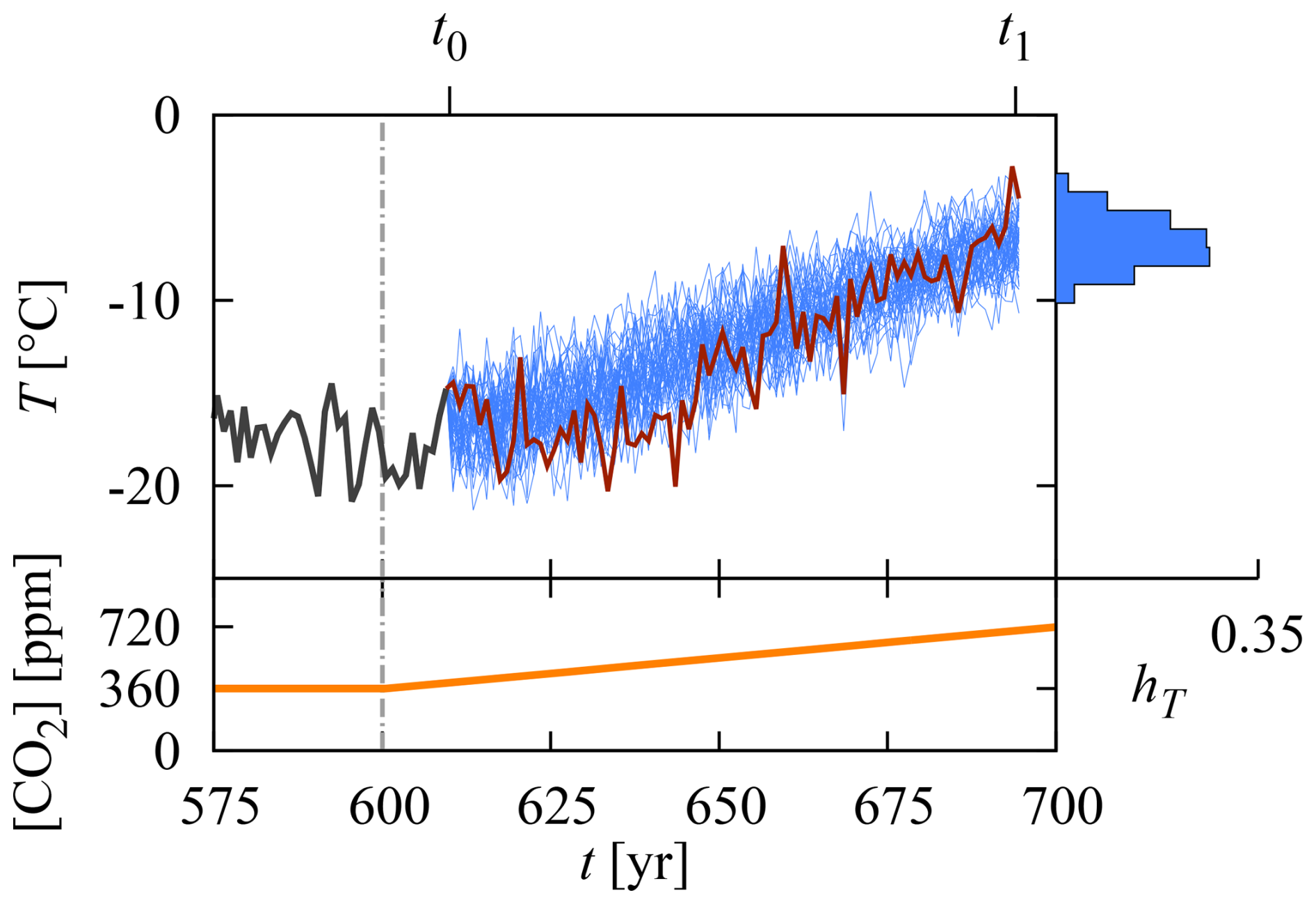
Figure C1 The annual mean near-surface temperature T of a single grid point in the southern Pacific Ocean (at 180° E and about 64° S) as a function of time. t₀=610 years is identified with the present, and t₁=694 years is an (almost) arbitrarily chosen year in the future. The dark gray line is a single PlaSim simulation and is regarded as the instrumental record in the model system. The red line is the continuation of the same simulation and is regarded as a prediction. The 48 light blue lines are alternative predictions, obtained from simulations initialized by slightly perturbing the surface pressure field of the simulation of the dark gray line at t₀=610 years (see the main text and Drótos et al. (2017) for details). The normalized histogram h_T constructed from the 48 values of the light blue lines and further 144 alternative predictions (a total of 192 values) at t₁ is shown on the right-hand-side of the main plot. The CO₂ concentration, through which the forcing scenario is defined, is also displayed (in orange). The vertical dot-dashed line in gray marks the beginning of the linear ramp in the CO₂ concentration. Data are from Drotos (2022).

A possible question about the weather of the future is, to take an (almost) arbitrarily chosen example, say, what the near-surface temperature at the given grid point will be at t₁=694 years. To obtain this temperature, we can use the t=t₀ phase space position of the dark gray trajectory of Fig. C1 as initial condition, and integrate PlaSim from t₀ to t₁: the result for the near-surface temperature of the given grid point is the red trajectory shown in Fig. C1, which has, of course, a unique value at t₁. However, this value is only one possible answer to the question.

Let us slightly perturb the t=t₀ phase space position of the dark gray trajectory 192 times to obtain 192 different initial conditions: the utilized random perturbation modifies the surface pressure field on the order of 10⁻³ hPa (see again Drótos et al. (2017) for the details), so that each perturbed initial condition can be regarded as realistic as the original one. In particular, these different initial conditions could not be distinguished by standard instrumental measurements on the real Earth (cf. de Melo Viríssimo and Stainforth, 2025). The integration of PlaSim from these initial conditions results in an ensemble of trajectories, plotted in light blue in Fig. C1 (only 48 of the 192 for better visibility), each giving a separate answer for the weather at t₁. All are possible answers, and the differences between them emerge as a result of the chaotic nature (unpredictable internal variability; Herein et al., 2023) of the system.

In fact, infinitely many of these answers would trace out a density, as indicated by the normalized histogram h_T in Fig. C1. We can ask now if this density provides a relevant characterization of the plethora of all possible near-surface temperature values at t₁.

In particular, the question is about the uniqueness of this density. If we perturb the original initial condition at t₀ in a different way, will we end up with a different density at t₁? For example, if we take a larger or a smaller magnitude for the perturbation, will the final density be broader or more narrow? Or if we restrict the sign in the perturbation, will it shift the final density in some direction? Since the initial conditions can never be constrained to arbitrary precision, such perturbations can be regarded just as relevant as the original one.

In fact, for an infinitely large ensemble in a dissipative nonautonomous dynamical system exhibiting chaotic behavior (such as PlaSim), the kind of density in question corresponds to the natural probability measure of a snapshot (Romeiras et al., 1990) or pullback (Ghil et al., 2008; Chekroun et al., 2011) attractor if t₀ tends to −∞, at least as long as the initial conditions remain in the basin of attraction of the same attractor¹². The density of the natural probability measure is unique, i.e., it will be the same for any generic set of infinitely numerous initial conditions within the basin of attraction of the given attractor. As we discussed in Appendix A, an atmospherically motivated toy model was used in Drótos et al. (2015) to illustrate that a process of convergence to the natural probability measure (forward in time) is exponential-like on the long term (it is presumably faster than any power law, cf. Appendix D). In such a case, the convergence of a finite-size ensemble is practically accomplished (with “exponential precision”, according to some practical point of view; see later) within a finite amount of time. In Herein et al. (2016), this was found to be the case for PlaSim, too, and this finding was conjectured to be relevant to any global climate model or Earth system model. In our configuration of PlaSim, the convergence time proved to be a few decades.

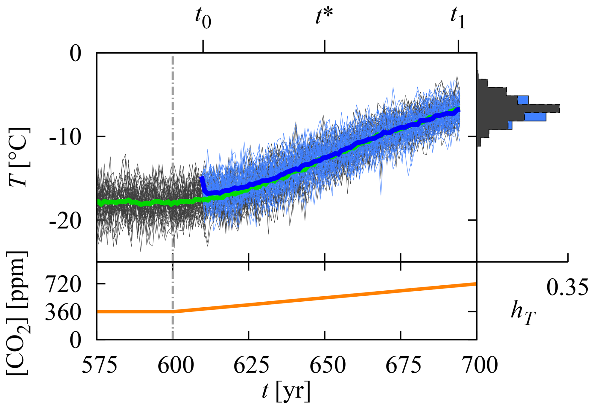
Figure C2 The light blue lines and histogram of Fig. C1 compared with an ensemble of the same size (marked by dark gray) initialized in the remote past (at t=0, asymptotically far in practice from t=575 years). The corresponding ensemble averages are also shown in dark blue and green, respectively. By t^*, the two ensemble averages practically coincide. Data are from Drotos (2022).

As a consequence, the probability density of the near-surface temperature at the investigated grid point in our configuration (and that of any other variable or set of variables) that is traced out by even a finite-size ensemble at t₁ will be practically the same regardless of how we choose initial conditions at t₀ – provided that two conditions are met. The first one is that t₀ has to be sufficiently far, although not infinitely far, in the past from t₁. The second is that the initial conditions must be chosen within such limits that ensure convergence to the desired attractor, avoiding a different one, e.g., a snowball Earth (cf. Kaszás et al., 2019; Ragon et al., 2022). Since t₀ and t₁ are separated by several decades in Fig. C1, this conclusion translates for our example as follows: within the mentioned limits, we cannot modify the initialization scheme at t₀ to obtain a substantially different probability density at t₁; that is, within a certain range of initialization schemes, we cannot “ruin” the quantitative result. Among other initialization schemes (which need not rely on some particular trajectory of the system), an extremely small perturbation of the actually realized initial conditions (the t=t₀ phase space position corresponding to the dark gray line of Fig. C1 in our model Earth system, the equivalent of hypothetical perfect instrumental observations at t₀ in the real Earth system) will lead to this unique density, which corresponds to the natural probability measure, see Fig. C2.

These considerations suggest this unique density (the natural probability density, in what follows) to be the practically relevant a priori (Paillard, 2008) probability density (i.e., existing independently of almost any observation about the system) that can be associated with the plethora of all possibilities at a future time instant t₁ that are permitted by the dynamics under the given forcing scenario (within the relevant basin of attraction, being the only observational constraint). That is, beyond being of practical interest, the natural probability density basically characterizes the system in statistical or probabilistic terms, instead of characterizing a particular situation (a “microstate” in a statistical mechanical analogy, e.g., a weather configuration in the atmosphere¹³) permitted by the system. Note that this abstract density exists at any time instant: not only at t₁, but also after and even before it (for instance, also at the time instant t₀ identified with the present, or even earlier; see the dark gray ensemble of Fig. C2). To practically obtain this density at a given time instant, one just needs to prescribe initial conditions for an ensemble in the sufficiently far past (within the relevant basin of attraction), and follow the time evolution of the ensemble until the desired time instant.

Of course, the natural probability density depends on time in the presence of a forcing (which is the generic situation and is so in the dynamics of the real Earth system; see again the dark gray ensemble of Fig. C2 for our model configuration). Otherwise, it is constant in time, and coincides with the natural probability density of the usual chaotic (stationary) attractor of the dynamical system (Ott, 1993).¹⁴¹⁵

We now recall that any definition of climate intends to capture statistical properties (including those related to temporal aspects). We also see that the relevant statistical properties of the system are, at root, described by the natural probability measure of the relevant snapshot or pullback attractor at any time instant. Therefore, we would hereby naively suggest defining climate as the statistical properties determined by the (infinitely large) ensemble of trajectories evolving according to the natural probability measure under a given forcing scenario. Then the expected value of some given variable will be the climatic mean value of that variable, and all higher-order moments will describe internal variability. With this definition, any particular realization of the dynamics will perform a sampling of the probability density that defines climate (i.e., the “climatological distribution” in the terminology of Branstator and Teng (2010)).

Appendix D: Identifying time scales of convergence

We discuss here how the spectral theory of transfer operators (Lasota and Mackey, 1994; Dellnitz et al., 2000; Slegers, 2019) should enable one to identify time scales of convergence.

Let us first consider an autonomous system, i.e., one without any explicit dependence on time, hypothetically describing a stationary climate:

$$\begin{array}{}\text{(D1)}& \dot{\mathit{x}}=\mathbf{F}\left(\mathit{x}\right),\end{array}$$

where x∈X represents the vector composed of all dynamical variables of the system, with X being the d-dimensional phase space spanned by these vectors, and F defines the dynamics, which is assumed to be dissipative. Let ${\mathcal{P}}_{t_{\mathrm{0}}}^t$ denote the Ruelle–Perron–Frobenius or transfer operator associated with the dynamics between time t₀ and t₀+t with t≥0 and defined with respect to the Lebesgue measure of X: the time evolution of probability densities f defined on X is described by the action of operators ${\mathcal{P}}_{t_{\mathrm{0}}}^t$ on f with different values of t≥0. If the operators ${\mathcal{P}}_{t_{\mathrm{0}}}^t$ are quasi-compact (i.e., if they have a finite number of isolated eigenvalues outside the essential radius; the universal belief that this is the typical case can be traced back to Keller and Liverani (1999); Blank et al. (2002)), the time evolution of an arbitrarily initialized probability density f from the class of square-integrable functions on X can be decomposed as

$$\begin{array}{}\text{(D2)}& {\mathcal{P}}_{t_{\mathrm{0}}}^t\left(f\right)=\sum _{i=\mathrm{1}}^N{c}_i{\mathit{\lambda }}_i^{t/T}{\mathit{\phi }}_i+r\left(t\right),\end{array}$$

where c_i, $i\in \mathit{\{}\mathrm{1},\mathrm{\dots },N\mathit{\}}$ are constant coefficients depending on f (such that c₁=1), T is the unit of time, N is the number of isolated eigenvalues of the operator ${\mathcal{P}}_{t_{\mathrm{0}}}^T$, λ_i is the ith of these eigenvalues with λ₁=1 and $\left|{\mathit{\lambda }}_i\right|<\mathrm{1}$ for all $\mathrm{1}<i\le N$ (note that these eigenvalues are generally complex and come in complex conjugate pairs), φ_i is the ith eigenfunction of the same operator (note that φ₁ is the density of the natural probability measure), and r(t) is a residual decaying faster than ${\mathit{\lambda }}_N^{t/T}$ (Györgyi and Szépfalusy, 1988; Chekroun et al., 2014; Slegers, 2019; Navarra et al., 2021). If there are multiple attractors, which have separate basins of attraction in the phase space, the decomposition (D2) applies separately to densities f with an initial support falling in a single basin (Tantet et al., 2018a).

Equation (D2) means that f converges to the density φ₁ of the corresponding natural probability measure, and the convergence proceeds according to exponential terms with different time scales of decay, as per the real parts of the eigenvalues and accompanied by oscillations as determined by the imaginary parts, and a fast-decaying residual. The exponential contributions with different decay time scales may then form the basis of the conditional definition of climate: if the separation between decay time scales is sufficiently large, “complete” convergence is possible on one time scale without an influence from processes with longer convergence time scales. From a technical point of view, what remains after such a “complete” convergence is a projection of the initial density f obtained by omitting the fast-converging terms in the decomposition (D2); eventually, this would be the mathematical object defining climate in an autonomous system.

A time scale of convergence may (possibly) be associated with a particular system component according to properties of the corresponding eigenfunction. Furthermore, the multivariate density shows how much fluctuations in different system components are correlated.

An important remark to be made here is that time evolution associated with a given eigenfunction may very well happen to be fast according to the oscillatory part, even if the corresponding decay is slow. In such a case, fast time evolution is predictable, as the autocorrelation function can be decomposed in terms of the same modes (one may refer, e.g., to Corollary 1 in Chekroun et al., 2020, which addresses a similar setup); cf. Sect. 2.

While the above considerations concern autonomous systems, generalization to periodically forced systems is easy by identifying the unit T of time with the period of the forcing. In this case, Eq. (D2) will hold for t=nT with n∈ℕ. Similar results also exist in systems with nonperiodic dependence on time (Froyland et al., 2010), but the eigenvalues are not constant in this case. Although tippings (Ashwin et al., 2012), especially crises of corresponding stationary chaotic attractors (Tantet et al., 2018a, b), may lead to complications at least for some eigenvalues, if most of the eigenvalues vary moderately enough, as might be expected under forcing scenarios relevant to century-long studies, these eigenvalues remain informative about the time scales in the system (cf. Tantet et al., 2020). An attempt for computing an approximation of the spectrum of the relevant transfer operator is nevertheless beyond the scope of this article.

We mention that more sophisticated and, at the same time, more easily implementable techniques also exist for identifying some kinds of time scale separation; see, e.g., Froyland et al. (2014, 2016), and cf. Lucarini and Chekroun (2023). In contrast, our application appears to necessitate a very specific notion, for which these techniques are not sufficient: an explicit gap in the real part of the eigenspectrum.

Appendix E: Regime transitions and uniqueness in slow-fast systems

For simplicity, we use a slow-fast system in the terminology of (Kuehn, 2015). In particular, we use the Itô stochastic differential equations of motion

$$\begin{array}{}\text{(E1)}& {\displaystyle }\mathrm{d}x=(-x^{\mathrm{3}}+\mathrm{2}x)\mathrm{d}t+{\mathit{\sigma }}_{xx}\mathrm{d}{W}_{xx,t}+{\displaystyle \frac{\mathrm{1}}{\mathit{ϵ}}}{\mathit{\sigma }}_{xy}y\mathrm{d}t,\text{(E2)}& {\displaystyle }\mathrm{d}y={\displaystyle \frac{\mathrm{1}}{{\mathit{ϵ}}^{\mathrm{2}}}}(-y+cx)\mathrm{d}t+{\displaystyle \frac{\mathrm{1}}{\mathit{ϵ}}}{\mathit{\sigma }}_{yy}\mathrm{d}{W}_{yy,t},\end{array}$$

to demonstrate that an ensemble initialized by small perturbations during a regime transition cannot represent climate in the absence of its uniqueness on the short term. A time scale separation between the slow x and fast y variables is achieved as ϵ→0 (Wouters and Gottwald, 2019). To represent a practical, realistic situation, we set ϵ=0.2. The slow subsystem is characterized by a symmetric quartic polynomial potential function like in Bódai (2020). It is perturbed both by some noise (σ_xx>0) and the fast subsystem (σ_xy>0), which latter features (internal) variability generated by white noise (σ_yy>0) (Hasselmann, 1976; Wouters and Gottwald, 2019). Effectively, the time scale separation between y and some even faster z whose governing equation is eliminated is readily represented in the stochastic model. The noise dW_xx,t is the slow subsystem's own internal variability, unaffected by the fast subsystem. The fast variable is affected by the slow variable (c≠0), which is why when climate cannot be defined with respect to the slow variable, it carries over to the fast one. We use the parameter values of σ_xx=0.6, σ_xy=0.4, σ_yy=1, c=0.2. The equations are integrated by the Euler–Maruyama integration scheme, using a time step of Δt=0.02.

The quartic polynomial represents a double-well potential function and so gives rise to a saddle-type unstable fixed point, i.e., a saddle, at $x=y=\mathrm{0}$ in the unperturbed (${\mathit{\sigma }}_{xx}={\mathit{\sigma }}_{yy}=\mathrm{0}$) 2D system (E1)–(E2), also called a Melancholia state in Lucarini and Bódai (2020), whose stable manifold makes a finite angle with the x=0 line owing to the coupling σ_xy>0. With a weak perturbation (in the sense of Bódai, 2020), infrequent transitions between the potential wells, across the Melancholia state, take place in terms of a long single-realization “control” run.

In order to examine the uniqueness of the converged ensemble, we initialize a pair of ensembles at some state of the control run. Namely, we “perturb” the fast variable as y+δy, $\mathit{\delta }y=+\mathrm{1}$ for one ensemble and $\mathit{\delta }y=-\mathrm{1}$ for the other ensemble.¹⁶ We do so in order to have two markedly different¹⁷ ensembles initially – the difference of the emanating densities has to disappear on the fast time scale to allow for a unique definition of climate. When the dynamics is deterministic, a minute mismatch of the initial conditions within each of the ensembles – at least with respect to z – is needed for the spread of that ensemble. In our stochastic modeling, however, it is clearly not required. The various different realizations of the ensemble members are generated by various different realizations of the Wiener process W_yy,t.

Given the said inclination of the stable manifold, which is the basin boundary of the unperturbed system, the opposite perturbations y±δy, even if taken in the y-direction only, could already achieve the placement of the two initial conditions in the different basins of attraction, provided that the current (x,y) was not far off from the basin boundary. Then, ensuing perturbed (σ_yy>0) realizations will much more likely end up in the near future in the potential well/regime where they started out from. As only the fast variable is perturbed to initialize an ensemble, the same single realization of W_xx,t of the control run is used for all of the ensemble members. In effect, this gives rise to nonautonomous dynamics, i.e., explicit time dependence in the system. Therefore, it is the stable manifold of the corresponding snapshot saddle that will actually control the transitions (Bódai et al., 2013).

When we initialize the two ensembles during a transition (see the middle row of Fig. E1), the ensemble means of neither the fast nor the slow variable, 〈y〉 and 〈x〉, converge but remain well separated, indicating the lack of uniqueness, at least on the time scale of the fast variable y. I.e., the realized ensemble will depend on the particular initialization of the fast subsystem. This indeed prevents any of these to objectively represent climate. On the contrary, when we initialize the two ensembles sufficiently far away from a transition, whether before or right after it (see the top and bottom rows of Fig. E1, respectively), the ensemble means converge on the time scale of the fast variable, indicating uniqueness. Due to the “forcing” of the slow subsystem, W_xx,t, clusters of trajectories (a subset of all of the trajectories because of σ_xy>0) suffer a regime transition in a coordinated manner, which is imprinted on the evolution of the ensemble means. That is, had the toy model reflected realistic characteristics of the climate system, regime transitions of the slow subsystem could give rise to the delineation of the concepts of climate change and forced response.

The case of σ_xx=0, when the slow subsystem does not have an internal variability in isolation from the y system component, is qualitatively similar: there is no uniqueness on the fast time scale in association with initialization during a regime transition of x.

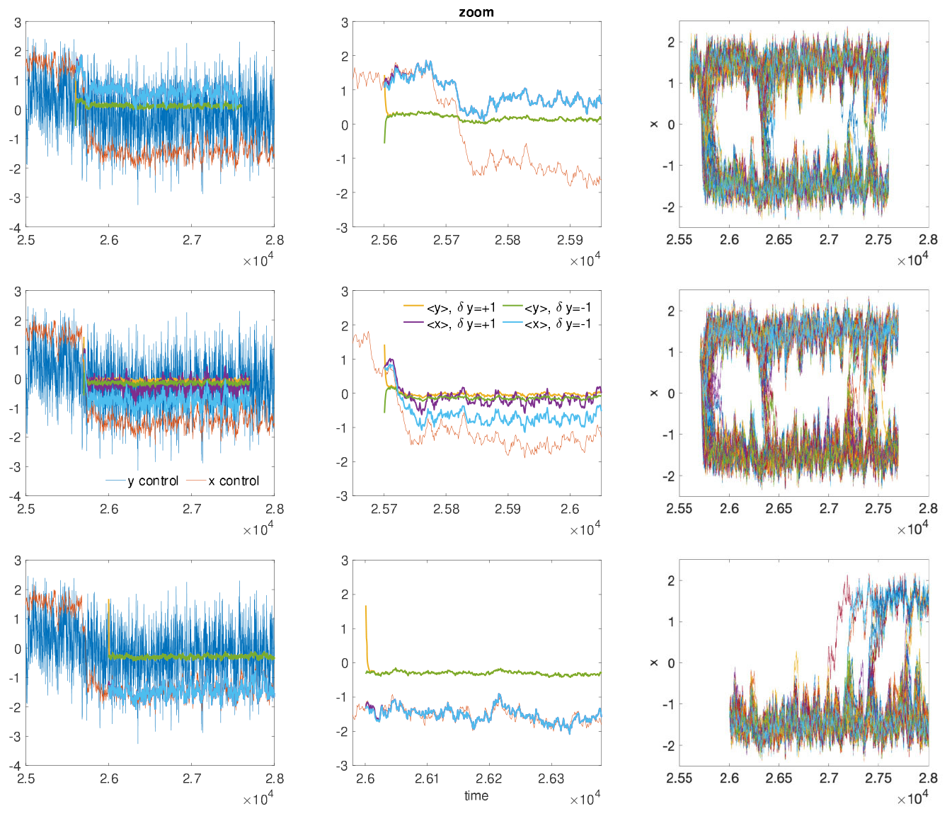
Figure E1 Initialization during and away from a regime transition precludes and supports the definition of climate, respectively. Two ensembles are initialized by perturbing the fast variable as $y+\mathit{\delta }y,\mathit{\delta }y=+\mathrm{1}$ or −1 (see main text), upon which the ensemble means 〈y〉 or 〈x〉 are plotted in diagrams on the left to examine convergence, using 1000 ensemble members in each ensemble. Diagrams in the middle column provide zoomed pictures of those on the left with respect to time, excluding the y control time series, for the better visibility of uniqueness. The legend annotations in two panels apply to all in the left and middle columns. On the right, spaghetti diagrams of all of the 1000 slow time series are given for one of the ensembles ($\mathit{\delta }y=+\mathrm{1}$). Data were produced by code by Bodai (2022).

Appendix F: The conditional definition in the Earth system: discussion

The main focus of this discussion will concern the real Earth system and its realistic models from the point of view of the possible conditional definition of climate introduced in Sect. 2.

We begin with acknowledging that we have no definite conclusion at present about the possibility of applying this definition. This is so because a major separation of time scales of convergence is not obvious in the real Earth system and in realistic models thereof; which, among other reasons, is so because time scales specifically characterizing convergence have rarely been assessed in these systems.

Having said that, we illustrate through the example of the ocean that our concept nevertheless gives guidance already to decide what can possibly be regarded as climate and what cannot in a given context. For an appropriate assessment of the issue, we need to reiterate from Sect. 2 that covering “complete” variability must always be defined in terms of some practical criterion, according to the exponential-like nature of convergence.

Studies about response time scales in the ocean (which is a different but related property) suggest, on the one hand, that time scales associated with the mixed layer and with layers below the thermocline are separated by a factor of about 10, and there might be no other characteristic time scale in between (e.g., Li and Jarvis, 2009; Olivié et al., 2012).¹⁸ Importantly, dynamical modes such as the Atlantic Meridional Overturning Circulation (AMOC; Buckley and Marshall, 2016) or the Atlantic Multidecadal Oscillation/Atlantic Multidecadal Variability (e.g., Delworth et al., 2007) do not seem to introduce complications, see later. Such a separation might or might not be just enough to treat the deep ocean separately from the rest of the system: by the time “complete” variability would unfold in the mixed layer (in terms of its own time scales), possibly unpredictable variations in the deep ocean might just become large enough to be relevant for an appropriate description.

On the other hand, one characteristic time scale of the unfolding of variability can be supposed to be a few decades according to the results from Li and Jarvis (2009); Olivié et al. (2012), which has recently been explicitly confirmed by Deser et al. (2025) with regard to AMOC: the authors report a convergence time (until convergence becomes practically complete) up to about 40 years. Therefore, it is clear that the variability associated with this convergence time at least needs to be regarded as the internal (chaotic) variability of climate, at least in studies concentrating on time spans around a century (as pointed out by Deser et al. (2025) as well). In terms of the definition of DelSole and Tippett (2018), a lead time of a few decades is required at least, and any shorter choice will inhibit a satisfactory interpretation of corresponding results.

Whether the unfolding of (unpredictable) variability on longer time scales is required to be taken into account remains an open question, according to what has been previously discussed. While a separation by a factor of 10 may rather suggest an answer of “no”, it is unclear why the intermediate time scale of the Atlantic Multidecadal Oscillation/Atlantic Multidecadal Variability, if such a mode exists (Vincze and Jánosi, 2011; Mann et al., 2021), does not appear in the referenced analyses and what role it plays in the unfolding of variability. We emphasize it here that the numerically observable time scales may depend on the particular choice of a variable.

Actually, one may also think of situations with little correlation between fluctuations of different system components, for which an example might be the relationship between the deep ocean and the surface-related processes, in which case the unfolding of deep oceanic variability would be irrelevant for most observables of practical interest. According to recent research (Singh et al., 2022), there are some signs that suggest this to be so for most of the globe but not for the Southern Ocean.

To be precise, time scales of convergence may not necessarily be associated with given system components or variables considered explicitly in the equations of motion. In this respect as well, one should rely on the framework discussed in Appendix D. This concerns also the degree of correlation between the internal variability of different system components; although, as explained in Sect. 2, this is presumably relevant only to how a (model) state should be chosen for initialization (attending to the predictable context).

One also has to consider the possibility that the real Earth system or some realistic model thereof does not meet the prerequisites of the description of convergence described in Appendix D. Long-term persistence (polynomially decaying autocorrelation) and, more generally, scaling of fluctuations in climate-related time series are reviewed by Franzke et al. (2020); see Lovejoy (2023) for more details about the phenomenology as applied to and observed in the present context. As pointed out in Sects. 2.3 and 5 of Franzke et al. (2020), long-term persistence and scaling may be illusory or they may result from external forcing, which would be in harmony with the Markovian nature of (most of the) equations of motion.¹⁹ In any case, if there is a break in the power spectrum such that there is a non-scaling regime of considerable length beyond the break (as, e.g., in Vincze and Jánosi, 2011), the decomposition of the convergence to (a generalization of) eigenmodes (as detailed in Appendix D) may retain its pertinence. While we have not identified relevant numerical modeling studies affected by the scaling issue, and the real-world Earth system may also be expected to be “well-behaved” at least in the sense last mentioned, real-world observational data as well as some theoretical aspects warn about possible complications (Franzke et al., 2020; Lovejoy, 2023). Careful future work, well beyond the scope of the present article, should address the question to what extent scaling laws in fluctuations have a spurious origin and which temporal or spatial scales are affected (and why) by scaling laws genuinely arising from the Earth system's dynamics, and why model studies remain unaffected if they do so indeed.

Before summarizing, we need to take care about the issue of regime behavior as raised in Sect. 2. Actually, the absence of different qualitative behaviors in global variables between members of currently existing large ensembles suggests that such an effect is restricted to particular system components at most. Such an effect might nevertheless appear in some slow system components (possible examples are related to Labrador Sea ice cover (Danabasoglu et al., 2020) and Southern Ocean variability (Gnanadesikan et al., 2020)), and uniqueness might or might not be lost in these cases: it depends on the way or the time of initialization. Cf. the illustration in Appendix E. Notably, such an effect should be easy to identify, e.g. following our proposal in Appendix G.²⁰

Taken together, we can say that distinguishing between different time scales of convergence appears to be reasonable to be expected to provide a sound definition of climate in the sense of Sect. 2: from the point of view of century-long investigations, we might expect to be able to meaningfully define climate through the probability measure obtained after a convergence time of a few decades (perhaps up to four, cf. Deser et al. (2025)). Further gaps in the spectrum of convergence time scales may possibly give rise to sound definitions for investigations on other time scales as well, but whether such gaps exist is a fully open question at present.

Appendix G: An initialization scheme: description

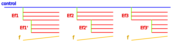
We propose the following ensemble initialization scheme, pictured in Fig. G1, for the purpose of deciding in a given model subjected to a given forcing whether a (practically) unique probability density typically appears in a given variable or (derived) observable within a time span of interest, and whether the state of slower-converging modes is relevant in an affirmative case.

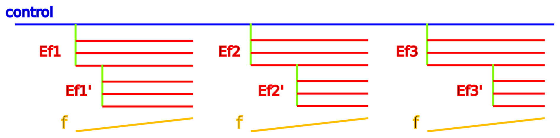
Figure G1 Illustration of the initialization scheme proposed in the main text. The horizontal axis stands for time. The vertical axis differentiates between ensemble members which are represented by horizontal lines; these ensemble members are grouped according to the labels Ef1, Ef1', etc. The blue realization (i.e., the control run) is unforced, whereas the red ensemble members are subject to the forcing scenario labelled by f and schematically represented in orange beneath the corresponding ensemble members. Note that the forcing scenario is continued without any interruption (e.g., any kind of restart) when initializing the ensembles with a label with a prime (Ef1', etc.). Vertical light green lines indicate minor perturbations. Unforced ensembles are not covered by this schematic.

In the first step, a single ensemble, Ef1, is initialized by small perturbations of a model state taken from a long control run. The trajectories of Ef1 are then integrated under the forcing of interest (typically the historical forcing followed by some future scenario such as SSP3-7.0 (Gidden et al., 2019)). The next step is the initialization of a second ensemble, Ef1', by perturbations of a model state taken from an arbitrary member of the first ensemble, Ef1, similarly as in Herein et al. (2023). The delay in its initialization should be around the shortest time scale for which one may first be interested in convergence and uniqueness. Then the same procedure is repeated for a few further time instants of the control run, resulting in additional ensemble pairs (Ef2,Ef2'), (Ef3,Ef3'), etc., such that Efn is separated from Ef(n−1) more than the length of the time span of interest (thereby sampling different states of modes with comparable convergence times at least). However, the pairs with subsequent indices n are different in that the delay in the initialization of Efn' with respect to Efn increases with n until the full time span of interest is approached (at least).

In terms of a given variable, uniqueness can be assessed by evaluating whether Efn' converges to Efn, for various indices n, with regard to a practical aspect. In case Efn' converges to Efn for some given n with a shorter time scale (approximate or bounding e-folding time) than the delay between Efn' and Efn for the given n, a “full” convergence with that time scale ensures uniqueness if “full” convergence is also observed up to some index m with Efm' separated from Efm by that “full” convergence time at least. The largest such m will define the longest time span (perhaps the time span of interest or, if studied, even longer) for which climate can be defined with the given convergence time.²¹ Once convergence is noticed to take considerably longer (for indices beyond that just-mentioned largest m), it indicates unpredictability arising from modes with comparable time scales of convergence and precludes uniqueness for correspondingly long times.²²

By intuition, we suspect that investigating convergence to an ensemble that has already begun spreading out from localized initial conditions is technically easier, especially from the point of view of slower-converging modes, than to one initialized at the same time just localized around a different point in the phase space; this is one advantage of initializing Efn' from a member of Efn during an active forcing scenario rather than using a different time instant from the control run to initialize Efn' at the beginning of the scenario as well. This is also beneficial because properties of the convergence during the bulk of a forcing scenario may be different and have more practical relevance than those just after switching the scenario on. In fact, by virtue of the increase of the delay with n, different epochs within the scenario, possibly with different convergence properties, are covered by our scheme.

Having said that, however, we must note that our approach is not fully perfect as it does not explore such properties systematically and, at the same time, uses convergence with those possibly different properties for the assessment of the longest time span of a sound definition. In fact, it would be desirable to initialize many ensembles for each n at increasingly later time instants within the scenario, thereby introducing a new index serving for an assessment similar to but (by using later-initialized ensembles as additional references for convergence) more general than the one described earlier. Our scheme has been designed under the assumption, supported by some numerical experience (e.g., Herein et al., 2016), that convergence properties are not considerably different in different epochs of a climate forcing scenario.

Scenarios have a finite length. Even if it may reach beyond some given “time span of interest”, an assessment of arbitrary slower-converging modes (whether their mere existence or relevance to a given variable, implying issue (i) in an affirmative case) is only possible with the help of a control run. This is what can be performed by evaluating the convergence of ensembles Efn with different indices n to each other.

All of what is discussed above needs a word of caution: certain ensembles of the many may happen to be initialized from very similar states of some mode by chance, which will make the effect of this mode perhaps even invisible when considering the convergence of these ensembles to each other. Without actually knowing these modes, this risk is unavoidable. It can be mitigated by increasing the number of initialized ensembles and carefully checking any suspicious case.

On the other hand, if convergence of Efn' to Efn fails for a few but only few values of n without being clustered to high n, it presumably indicates the problem of regime transitions (or that of vicinity of basin boundaries; a violation of condition (b) in either case).

It is easy to amend the above scheme to study issue (ii). For this purpose, the ensembles Efn should be compared with ensembles generated with identical initialization but with no forcing (Eun; “f” and “u” stand for forced and unforced, respectively). Note, however, that model drift (Gupta et al., 2013) has the same effect from this point of view as a possible predictable evolution of slower-converging modes; but, at least, forced changes can always be discerned.

Our proposed initialization scheme is different from that of Hawkins et al. (2016), Hogan and Sriver (2019), the CanESM2 large ensemble (Kirchmeier-Young et al., 2017; Singh et al., 2022) and the CESM2 large ensemble (Rodgers et al., 2021) in that pairs of ensembles are initialized by perturbations in association with each model state taken from the control run, thereby enabling assessment of convergence to a (possibly conditionally) unique probability density. Timing of initialization is also important. On the one hand, different delays are used between the members of pairs for the just-mentioned assessment. On the other hand, different model states for different pairs are taken from far away time instants of the control run so that slower-converging modes, with respect to the time span of interest, can also be studied. Most of the cited studies target a century or so but apply a separation of just 50 years. Note that model drift (as in Singh et al., 2022) is not at all ideal for assessing the impact of the state of slower-converging modes (the predictable context) on the climate defined after convergence in faster-converging modes, due to its inherently artificial nature.