Land carbon response to positive, zero, and negative CO₂ emissions across Earth system models

Land carbon sinks are responsible for removing about a quarter of anthropogenic CO₂ emissions, and make up approximately half of total global carbon sinks. Uncertainty in the response of land carbon sinks to climate and changing atmospheric CO₂ are large, and dominate the uncertainty in total carbon sinks under future climate. Understanding the carbon cycle response to net-zero and net-negative emissions has important implications for projecting future climate. Here we characterize the response of land carbon pools and fluxes from ten emissions-driven Earth system models (ESMs) under positive, net-zero, and net-negative CO₂ emissions using experiments from the “flat10” model intercomparison. Although there are many differences in simulated land carbon pools and fluxes across models, we find some consistent behavior across ESMs. (1) During the positive emissions phase, carbon is gained on land primarily in vegetation pools. (2) Following net-negative emissions to the point of cumulative zero emissions, carbon is lost from land in tropical latitudes, primarily from vegetation pools, but in mid- and high-latitudes most models show net land carbon gain, primarily in soil pools. (3) Following an extended period of net-zero emissions, a majority of models again show carbon gain in mid- and high-latitudes and vegetation carbon loss in the tropics. Under net-negative emissions the timing of vegetation carbon response relative to peak emissions is relatively consistent across ESMs, but timing of soil carbon response varies widely, implying larger intermodel disagreement associated with responses of soil carbon which tends to have longer timescales relative to vegetation carbon. Our findings highlight that tropical carbon is most likely to be both gained and subsequently lost under positive, zero, declining, and negative emissions, with possible implications for carbon dioxide removal efforts.

1 Introduction

Terrestrial systems remove carbon from the atmosphere through photosynthesis, and release carbon through respiration, fire, and other pathways. The balance of these processes results in a net flux that represents either a source to or sink of carbon from the land to the atmosphere. Anthropogenic emissions of CO₂ into the atmosphere since the industrial revolution, including emissions from fossil fuel burning, cement production, and anthropogenic land cover and land use change, have been partially balanced by land and ocean carbon sinks, where here we define land sink as the net removal of CO₂ from the atmosphere by natural vegetation and agriculture. Over the industrial period, 755±65 Pg C of anthropogenic CO₂ has been emitted to the atmosphere (Friedlingstein et al., 2026). Of this, terrestrial carbon sinks are estimated to have removed about 24 %, or 175±50 Pg C, with 27 % going into ocean sinks and 39 % remaining in the atmosphere and leading to increased atmospheric CO₂ concentrations. Over the period 1959–2024 a 1 Pg C yr⁻¹ imbalance remains unattributed to specific fluxes in the assessed global carbon budget (Friedlingstein et al., 2026).

The net terrestrial carbon sink reflects the balance of many biologically mediated processes that depend on climatic conditions and atmospheric CO₂ concentrations. Leaf level photosynthesis has the potential to increase as the partial pressure of CO₂ in the atmosphere increases, at least at concentrations experienced up to this date (Bonan, 2015; Ficklin and Novick, 2017; Grossiord et al., 2020; Zhang et al., 2019). However, photosynthesis is also co-limited by irradiance, temperature, moisture stress, and nutrient availability; therefore, enhancement by increasing atmospheric CO₂ is limited. It is theorized that such limitations will become more widespread as temperatures continue to increase and rainfall patterns shift (e.g. Xu et al., 2019; Zhang et al., 2025), even considering possible acclimation of photosynthetic processes to temperature change (Yamori et al., 2014; Kumarathunge et al., 2019). Respiration releases carbon, both from autotrophic and heterotrophic sources. Generally respiration rates increase with warming, but acclimation may also moderate the response of respiration to temperature (Reich et al., 2016; Atkin and Tjoelker, 2003), and the specific rates also depend on microbial community composition (Wieder et al., 2013). The fact that land has served as a carbon sink during the historical period suggests that, to date, enhanced photosynthesis has outpaced increases in respiration.

Projections of future terrestrial carbon sinks by Earth system models (ESMs) were first systematically compared in modeling experiments that were part of the Coupled Climate Carbon Cycle Model Intercomparison Project (C4MIP, Friedlingstein et al., 2006), where the spread across models was large, and substantially larger than the spread across estimates of ocean carbon sinks. Many elements of the terrestrial carbon cycle are heterogenously represented, poorly understood and/or subject to significant parametric uncertainty, leading to these large divergences in model projections. The C4MIP effort has been repeated in the intervening years with newer generations of ESMs, but spread in estimated land carbon sinks across models has remained stubbornly large (Friedlingstein et al., 2014; Arora et al., 2020; Liddicoat et al., 2021). Not only is the spread in land carbon sink across models large, but the possible spread within a single model can also be substantial. For example, projections made with the CMIP3-era HadCM3 ESM spanned ∼450 ppm in atmospheric CO₂ in 2100 in response to modified assumptions within the land model (Booth et al., 2012), a behavior we expect would also occur in other ESMs. This lack of consensus across projections of the future land carbon sink likely stems from the fact that many biological processes contribute to the land carbon sink outcome, each of them remains individually uncertain, and the number of model implementations is very small compared the dimensionality of that uncertainty. We note that recent developments in model emulation and parameter constraints against data show some promise in restricting the range of projections (McNeall et al., 2024).

A new experimental design has recently been proposed and adopted for use in the coupled model intercomparsion project version 7 (CMIP7), called “flat10MIP” (Sanderson et al., 2025). The flat10MIP set of experiments uses emissions-driven ESMs to simulate the coupled carbon cycle response to specified idealized CO₂ emissions, including constant emissions near present-day rates, as well as an abrupt transition to zero emissions and a ramp-down of emissions to zero and then net-negative emissions. Prior experiments were based on specified concentrations of CO₂, diagnosing distinct emissions timeseries for each model. The flat10MIP experiments use specified emissions which allows for straightforward assessment of two climate metrics: the “transient climate response to cumulative CO₂ emissions” (TCRE, Allen et al., 2009; Matthews et al., 2009; Zickfeld et al., 2009; Meinshausen et al., 2009) which is the emergent near linear response of globally averaged surface temperature to the cumulative emissions of CO₂, and the “zero emissions commitment” (ZEC), which is the change in global mean temperature after annual emissions reach zero (Matthews and Caldeira, 2008; Solomon et al., 2009). Nine ESMs participated in the initial model intercomparison using this experimental design (see the methods section for details of the flat10 experiments, Sanderson et al., 2025). An assessment of TCRE and ZEC across the flat10MIP ensemble is presented in Sanderson et al. (2026).

Understanding the carbon cycle response to net-zero and net-negative emissions, and particularly the highly uncertain land carbon cycle response, has important implications for projecting future climate. The tendency for carbon sinks to become neutral or switch to sources under low emissions scenarios (Jones et al., 2016; Koven et al., 2022) is a key determinant of the coupled carbon-climate response to emissions, yet most model intercomparisons using emissions-driven ESMs have focused on regimes of increasing emissions, with only a limited number of simulations completed for lower or negative emissions scenarios (Asaadi et al., 2024).

The flat10MIP experiments offer a new opportunity to systematically compare the response of terrestrial carbon cycling to zero and net-negative emissions across a larger array of ESMs. TIPMIP (Jones et al., 2026) is another newly proposed intercomparison project with a goal of assessing ESMs at equal rates of warming. The TIPMIP experimental design uses ESM-specific emissions rates to achieve equal warming rates at a specified time point. The response of carbon cycling under equal rates of emissions (as in flat10MIP) may differ from the response under equal amounts of warming (as in TIPMIP).

Here we report responses of the flat10MIP experiments, focusing on characterizing the response of land carbon pools and fluxes to specified emissions in ten ESMs. A high-level analysis of changes in global ocean carbon budget in flat10MIP has been documented in Sanderson et al. (2025) and a detailed regional analysis is forthcoming. All ten ESMs performed the three flat10MIP scenarios, including positive, net-zero, and net-negative emissions (wherein all emitted carbon is removed to the point where cumulative emissions reach zero). In the methods we provide a description of the experimental design as well as broad differences across ESMs (brief descriptions of each ESM and descriptions of relevant components of their land carbon cycles are provided in the Appendix). In results and discussion we describe the initial carbon stocks in each ESM, their response to change during the positive emissions phase, net-zero phase, and during net-negative and at cumulative zero emissions. Finally, we present the timing of carbon pool responses relative to emissions under declining and negative emissions. We finish with conclusions and implications.

2 Data and Methods

2.1 flat10MIP experiments

The flat10MIP experimental design, described in Sanderson et al. (2025), consists of idealized experiments designed for directly and efficiently assessing TCRE and ZEC. Here we evaluate three flat10MIP experiments with a focus on land carbon stocks and fluxes (Fig. 1). The first is the “flat10” experiment (esm-flat10), wherein carbon is emitted to the atmosphere at 10 Pg C yr⁻¹. This experiment was continued for between 150 and 300 years depending on the ESM. At 100 years, the point where cumulative emissions are at 1000 Pg C, two experiments were branched. In the “flat10-zec” experiment (esm-flat10-zec), emissions are set to zero following the “flat10” increase, and the simulation is continued for 200 years. In the “flat10-cdr” experiment (esm-flat10-cdr), emissions decline by 0.2 Pg C yr⁻¹, reaching zero emissions at 50 years. Emissions then become negative and continue declining by 0.2 Pg C yr⁻¹ until reaching −10 Pg C yr⁻¹ at year 100. The simulation is continued for an additional 100 years at −10 Pg C yr⁻¹ emissions. Declining and negative emissions within flat10MIP are implemented in the same way as positive emissions, namely that they are idealized and do not have a spatial pattern. This idealized approach enables a general understanding of the reversibility of the climate system, but does not capture the co-occurring impacts of any particular carbon dioxide removal method (Zickfeld et al., 2023). Here we consider the esm-flat10-zec and esm-flat10-cdr experiments as a continuous time series with the initial 100 years from the esm-flat10 experiment, and the following 200 years from each of the protocols described above. Thus the point of zero emissions is reached at year 100 in esm-flat10-zec and at year 150 in esm-flat10-cdr. At year 300 in esm-flat10-cdr scenario, cumulative emissions over the whole time period have reached zero.

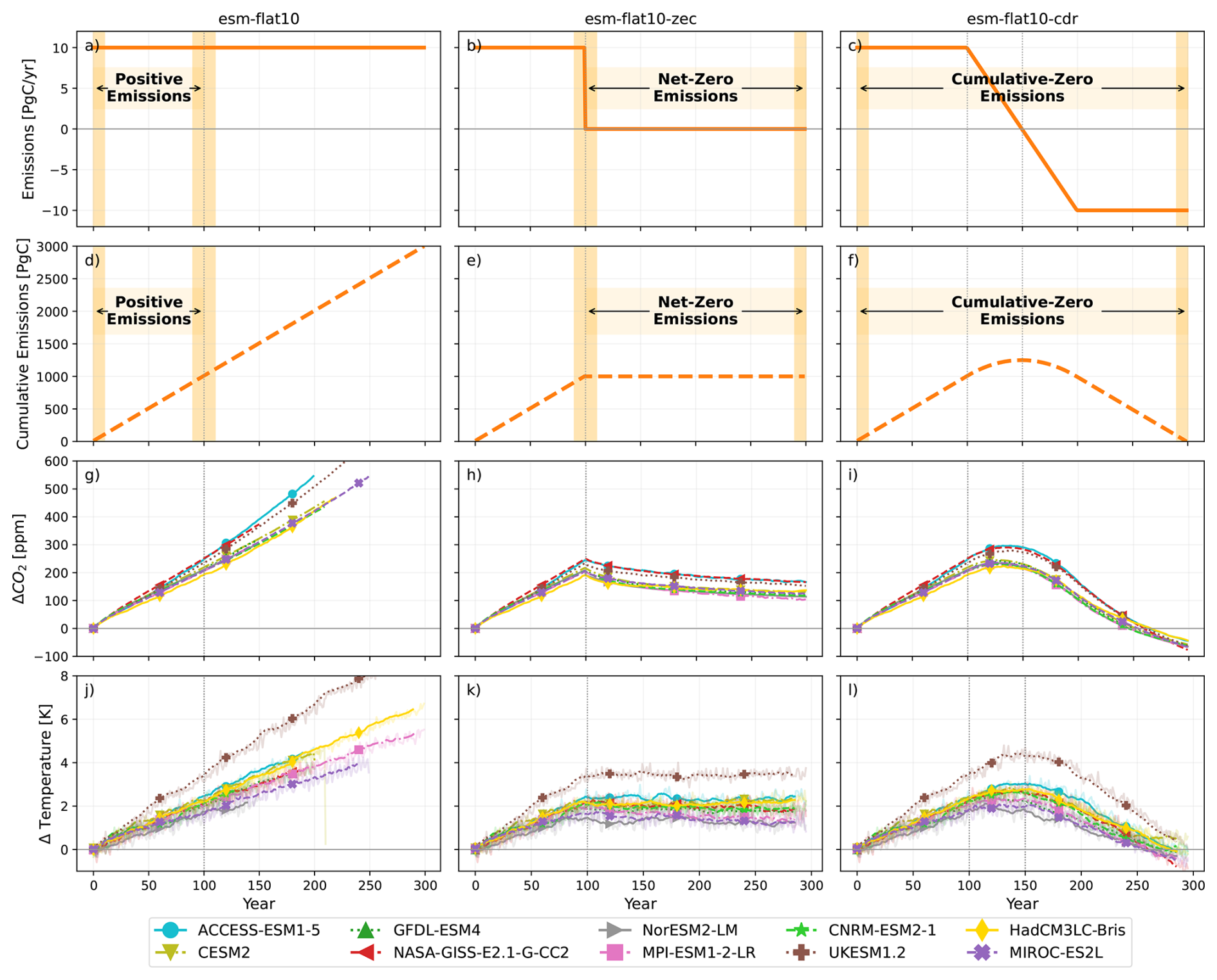
Figure 1 Global mean timeseries of emissions, cumulative emissions, temperature, and CO₂. Time series of annual emissions (top row), cumulative emissions (second row), change in global mean atmospheric CO₂ (third row), and temperature (smoothed with an 11-year running mean). Columns show each of the three experiments: esm-flat10 (left), esm-flat10-zec (middle), and esm-flat10-cdr (right). Each line in the second and third rows represents one ESM participating in flat10MIP. The vertical dashed lines indicate the year of 1000 Pg C of cumulative emissions, which corresponds to the year of net-zero emissions in esm-flat10-zec, as well as year 150 in the right hand column which is the year of net-zero emissions in esm-flat10-cdr. Shaded horizontal bars on the first two rows indicate the phases referred to throughout the main text, and vertical shaded bars indicate the time periods used to compute the change over each phase.

We analyze both the full time series as well as distinct time windows, or phases, within these simulations. Horizontal shaded bars in Fig. 1a–f indicate the duration and name of each phase, and vertical shaded bars indicate the time slices used to compute differences over those phases. We report initial carbon stocks (Initial C) as the average over the first 10 years of the esm-flat10 experiment. We report changes in carbon stocks around the end of the positive emissions phase (Δ Emissions Phase) as the difference between the average around 1000 Pg C of cumulative emissions in the esm-flat10 experiment (20 years centered on year 100) and the Initial C, while noting that this is the average over a transient period with increasing cumulative emissions for the first 10 years. We report the change in carbon following zero emissions (Δ Net-zero) as the average of around the end of the esm-flat10-zec experiment (last 10 years) minus carbon stocks at the end of the positive emissions phase (20 years centered on year 100). We report the change in carbon at cumulative zero emissions (Δ Cumulative-zero) as the average of the end of the esm-flat10-cdr experiment (last 10 years) minus the initial carbon pools.

2.2 Terrestrial carbon cycle representation in flat10MIP ESMs

Descriptions of the terrestrial carbon cycle representation within ESMs analyzed here can be found in the Appendix. Some processes relevant for terrestrial carbon cycling, such as nutrient limitation, vegetation dynamics, and complexity of soil carbon representation, and representation of fires vary across ESMs (Table 1).

Ziehn et al. (2020)Danabasoglu et al. (2020)Dunne et al. (2020)Shevliakova et al. (2024)Romanou et al. (2026)Kim et al. (2015)Seland et al. (2020)Mauritsen et al. (2019)Séférian et al. (2019)Delire et al. (2020)Valdes et al. (2017)Sellar et al. (2019)Hajima et al. (2020)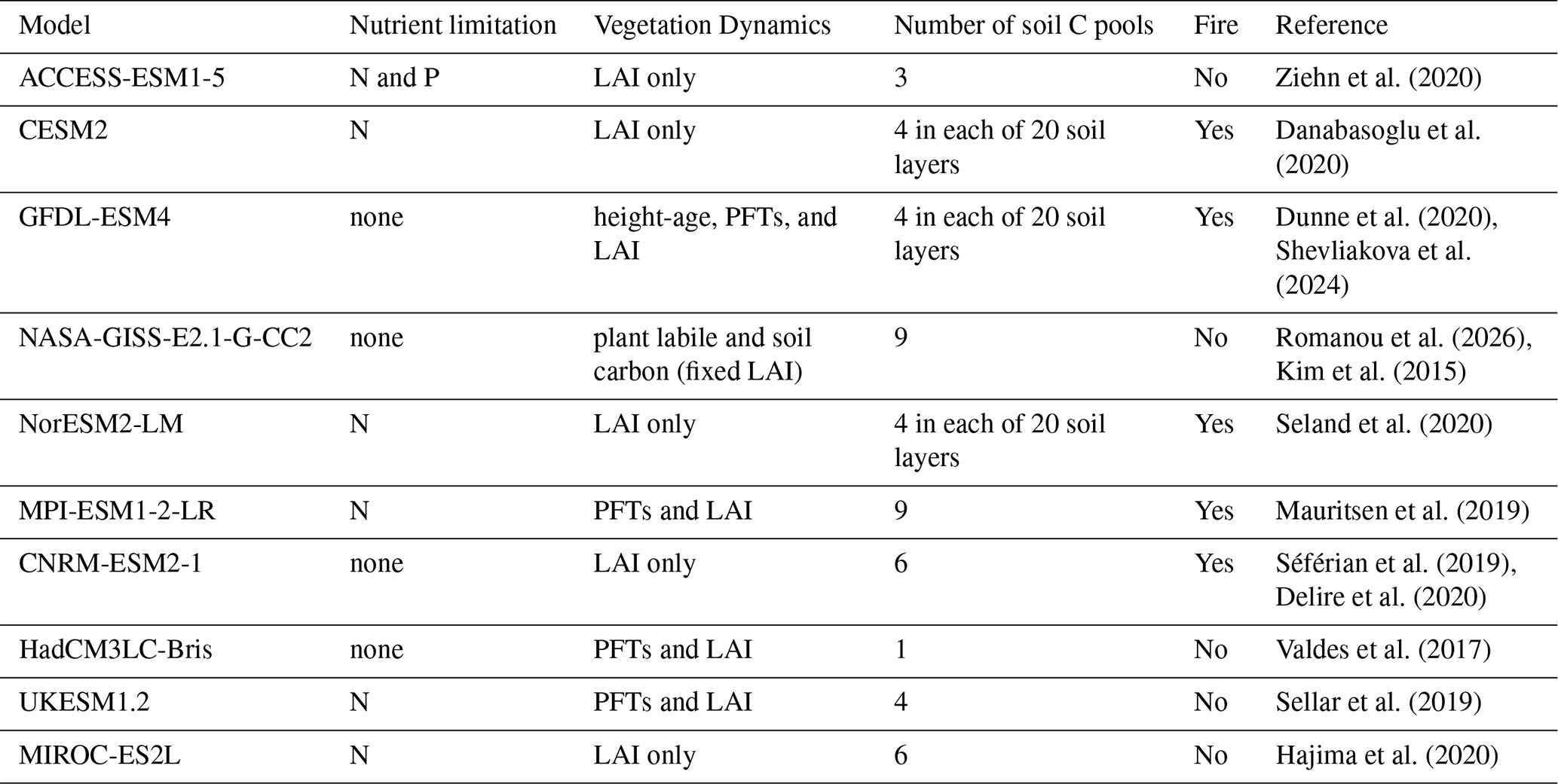

Table 1 Table of ESMs and relevant processes included in each.

2.2.1 Carbon pools

ESMs participating in flat10MIP report carbon content in either two or three land carbon pools. In each ESM, carbon within each of these overarching pools may be represented by many more sub-pools, however at most only three pools are reported in the tier-1 C4MIP variables that form the basis for CMIP carbon cycle reporting (Jones et al., 2016). Three of the ESMs analyzed here report only vegetation and soil carbon pools (NASA-GISS-E2.1-G-CC2, UKESM1.2, HadCM3LC-Bris), where litter carbon is implicitly included within soil pools. The remaining ESMs report vegetation, soil, and litter pools. We analyze all three pools distinctly when available, as well as the sum of all land carbon pools within each ESM, which we report as total land carbon.

Internally within each model many more carbon pools may be represented. We report the number of soil carbon pools specifically (Table 1), noting the wide diversity in number of pools represented across ESMs, which range from 1 in HadCM3LC-Bris to 4 within each of the 20 soil layers in CESM2, NorESM2-LM, and GFDL-ESM4, which results in a total of 80 soil carbon pools.

Of these ESMs, only CESM2, NorESM2-LM, and GFDL-ESM4 resolve soil carbon by depth (CESM2 and NorESM2-LM use CLM5 as their land component), which allows the separation of carbon in permanently frozen soil layers that may be thawed with warming from carbon that is actively cycling in shallow Arctic soils (Canadell et al., 2021, Table 5.4). Although both GFDL-ESM4 and the ESMs with CLM5 resolve soil carbon pools by depth they remain distinctly different models with independent development history.

2.2.2 Nutrient limitation

Six of the ESMs analyzed here represent nutrient cycling and nutrient limitations to photosynthesis. ACCESS-ESM1-5 is the only ESM in this study that represents both phosphorous and nitrogen limitation. An additional five of the ESMs represent nitrogen limitation: NorESM2-LM, CESM2, MPI-ESM1-2-LR, UKESM1.2, and MIROC-ES2L.

2.2.3 Vegetation dynamics

All of the land surface components within the ESMs used in this study have prognostic carbon cycles, where carbon pools are updated over time in response to dynamically calculated fluxes. All but one of the ESMs represent prognostically calculated dynamic leaf area, where the area of leaves per area of ground is an emergent property of the carbon cycle, typically the leaf carbon pool. The exception is NASA-GISS-E2.1-G-CC2, where leaf area is specified from a dataset that varies seasonally within a year but not across years, and carbon uptake that would be allocated to stem growth is transferred as litterfall to the soil pools, leaving the prognostic land carbon pools to be the plant labile storage and soil carbon.

Natural vegetation is specified in all of the ESMs represented here by discrete plant functional types, and no anthropogenic land use change occurs in the flat10MIP experiments. Plant types within a given gridcell are represented as either static in time or in some models as prognostically varying over time. Time-varying vegetation types are frequently referred to as “dynamic vegetation” (Cramer et al., 2001), although here we will use the term “dynamic biogeography” to differentiate variations in plant type from additional variations in plant age and size distributions. In GFDL-ESM4 plants are represented by cohorts of plant type and size-age, allowing for a more complex representation of ecosystem demographics and how they vary over time, which we term here a “demographic vegetation” model.

These various flavors of vegetation dynamics across models for leaf area, plant type, and plant demographics potentially contribute to the timescales and behavior of land carbon storage and fluxes.

2.3 Analysis methods

We report averages for different time periods within the simulations as described in Sect. 2.1 and shown in Fig. 1. We report zonal mean sums for three latitude bands: tropics (20° S to 20° N), mid-latitudes (>20 and <50°), and high-latitudes (>50°), as well as full zonal profiles. These particular boundaries of each latitude zone were selected because they broadly represent transitions between higher and lower carbon stocks across ESMs. When multi-model mean values are reported in the text we include the multi-model standard deviation or range across ESMs in brackets.

3 Results and Discussion

3.1 Carbon stocks

3.1.1 Initial carbon stocks (pre-industrial state)

Pre-industrial carbon stocks vary across ESMs in esm-flat10, both in total magnitude and in zonal distribution. The multi-model mean total global land carbon content is 1860 Pg [±568], with a range from the low end of 978 Pg C in GFDL-ESM4 and a high of 3119 Pg C in NorESM (Table A1). These esm-flat10 modeled estimates differ from the IPCC 6th assessment report (AR6) estimates for present-day carbon stocks which are 450 Pg C in vegetation, 1700 Pg C in non permafrost soils, and 1200 Pg C in permafrost soils, for a total global carbon budget estimate of 3350 Pg C on land (Canadell et al., 2021). The total estimated carbon in vegetation and soil excluding permafrost carbon reported by IPCC is 2150 Pg C (Canadell et al., 2021). IPCC estimates were made from a combination of approaches including modeling and present-day observations. We note that the comparison between pre-industrial with present-day conditions is not direct but provides a useful benchmark.

IPCC estimates suggest most present-day terrestrial carbon is in soils (87 % of total carbon in soils, 79 % if excluding permafrost). Most of the ESMs analyzed here also have the majority of carbon in the soil rather than vegetation, with 30 % [±8 %] in vegetation and 63 % [±13 %] in soil (Table A1), and no model having less than 17 % of carbon in vegetation. The relatively larger amount of carbon in soils compared with vegetation is consistent with other estimates of the global carbon cycle, however, the total magnitude of vegetation carbon pools is generally closer to the IPCC AR6 estimate, compared to the soil carbon pools. Overall, we find that a number of the ESMs have insufficient amounts of soil carbon relative to modern day observations (Fao, 2023; Jackson et al., 2017; Batjes, 2016; Hugelius et al., 2014; Canadell et al., 2021). In high latitudes specifically, a lack of sufficient carbon reflects that the representation of processes that govern carbon cycling in Arctic ecosystems is missing in most ESM soil models (Schuur et al., 2015, 2022; Natali et al., 2021; Matthes et al., 2025).

Regional evaluation of carbon pools and fluxes in CMIP6 models (Ito et al., 2020a; Jones et al., 2023) showed that there is a high diversity in performance across different regions and for different processes. Some models simulate fluxes better than pools and some vice versa. Some models perform well in some regions and poorly elsewhere. There were no clear “winners” in terms of models which performed well for all regions and all processes. It is likely the models used here, which are largely very closely related to CMIP6 versions, exhibit a similar mix of skill across regions and processes.

Many ESMs have similar amounts of carbon in tropical (<20°) and mid-latitudes (>20 and <50°) relative to high latitudes (>50°), with the notable exception of NorESM which has a very large high latitude carbon soil carbon pool. CESM2 has more high latitude carbon than mid latitude carbon, but not nearly to the same degree as NorESM despite these two models using the same land carbon cycle representation, albeit with slightly different calibrations (Figs. 2a–c, 4, 5, Table A2).

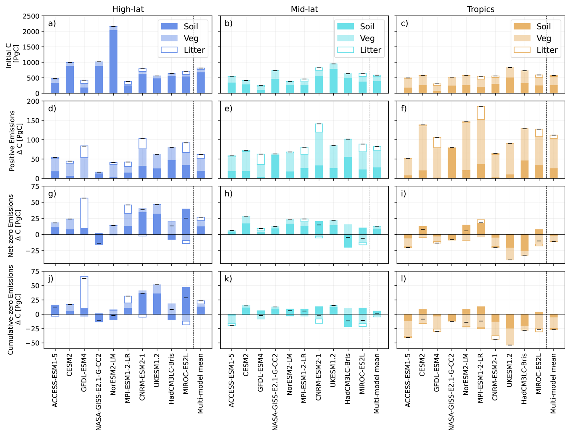
Figure 2 Carbon and Δcarbon at different latitudes. Bar graph showing initial carbon stocks (first row), and change in carbon stocks after positive emissions (second row), after net-zero emissions (third row), and after negative emissions (fourth row) in each of the ESMs participating in flat10MIP. Each column shows the initial stock or change in C for soil carbon (solid dark color), vegetation carbon (lighter color), and litter (white with outline) high-latitudes (>50°) in the left column, mid-latitude regions (>20 and <50°) in the middle column, and tropical regions (<20°) in the right column. Positive values are plotted above the zero line and negative values are plotted below the zero line. The total C (sum of all bars) is indicated with a black bar.

In the tropics ESMs simulate a large fraction of carbon in vegetation, with increasing relative amounts of soil carbon at mid- to high-latitudes (Fig. 2). Across all ESMs in mid-latitudes carbon stocks are >50 % in soil (except for GFDL-ESM4) and in high-latitudes carbon is mostly in soil (76 % [±14 %]), Figs. 4, 5).

The variation in global vegetation, litter and soil stocks across models are substantial (Fig. 2a–c). Given that soil and vegetation stocks require long spin-up and historical transient runs to reach a state which is comparable with present day observations, they are among the most challenging of targets for model calibration. This plausibly contributes to the wide variation of initial carbon stocks. Initial carbon stocks may also impact the response of carbon pools to perturbations as different initial carbon stocks also imply potentially different vulnerability to change because vegetation is typically represented as having a faster turnover time relative to soils. Thus an ESM with a larger fraction of carbon stored in vegetation could lose carbon more quickly compared to an ESM with relatively more carbon stored in soils. However, across this 10 member ensemble we do not see a robust relationship between initial carbon content and amount of carbon gained or lost during different phases (Fig. A1).

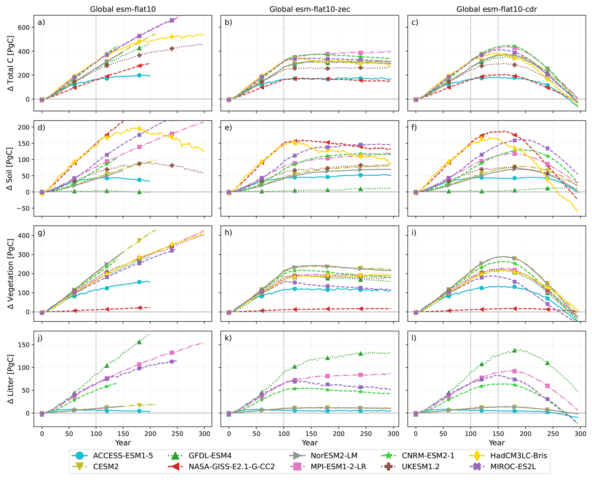
Figure 3 Global mean timeseries of carbon pools. Time series of global mean change in carbon stocks in each of the ESMs participating in flat10MIP in units of Pg C with total carbon in the top row, soil carbon in the second row, and vegetation carbon in the third row, and litter carbon in the fourth row (not all ESMs report litter). Columns show each of the three experiments: esm-flat10 (left), esm-flat10-zec (middle), and esm-flat10-cdr (right). Each colored line represents one ESM. The vertical dashed lines indicate the year of 1000 Pg C of cumulative emissions, which corresponds to the year of net-zero emissions in esm-flat10-zec, as well as year 150 in the right hand column which is the year of net-zero emissions in esm-flat10-cdr.

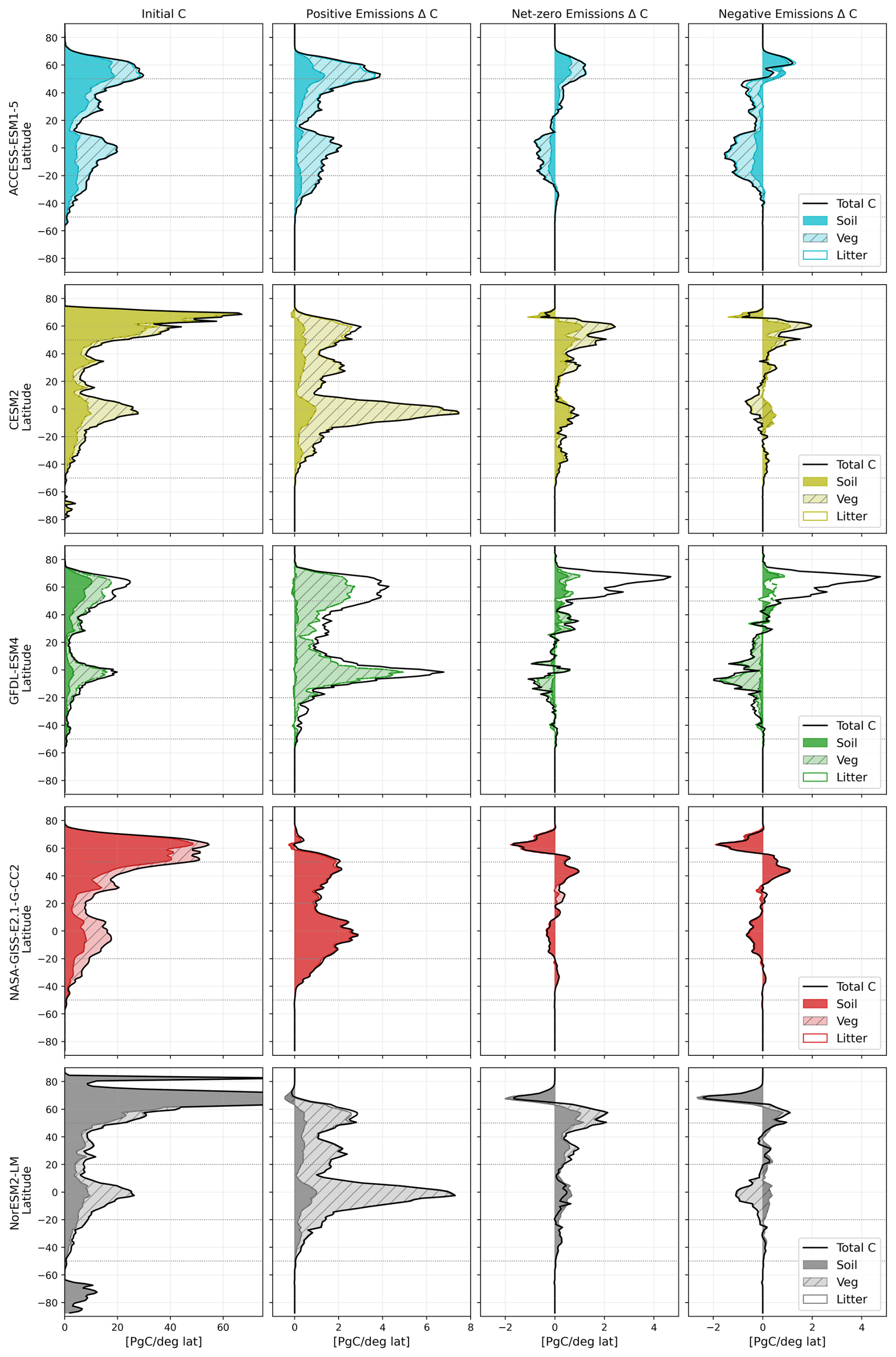
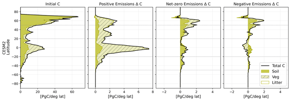
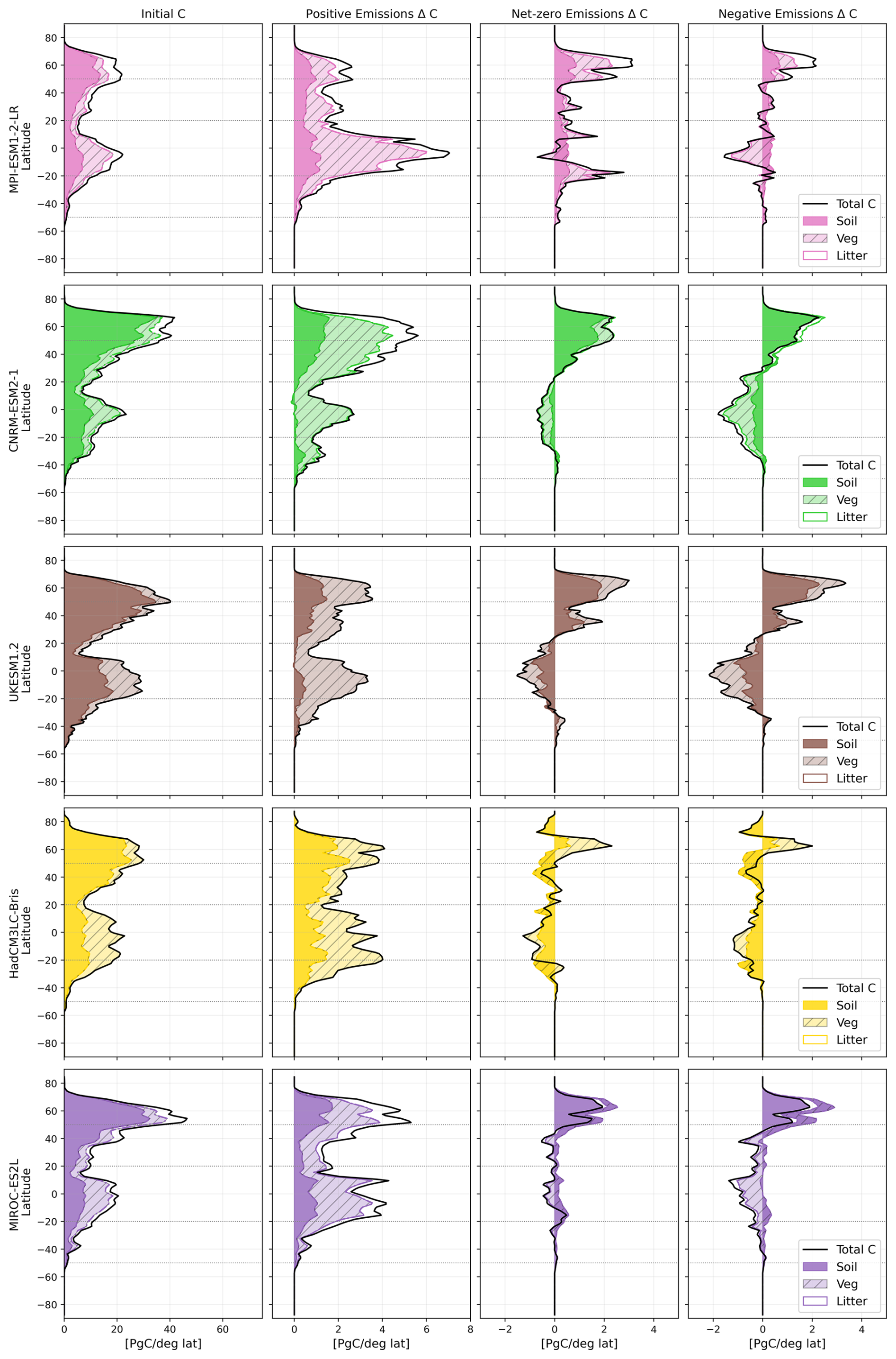
Figure 4 Initial C and ΔC at each emissions phase. Zonal initial carbon stocks and change in carbon stocks (columns) for a subset of the ESMs participating in flat10MIP (rows) in units of Pg C (remaining ESMs shown in Fig. 5) with one ESM shown on each row. The left column shows initial carbon stocks, the second from left column shows the end of the positive emissions phase, third from left column shows the net-zero phase, and right column shows the point of cumulative-zero emissions relative to the initial carbon pools. Total carbon pool is shown with a solid line, soil carbon pool in the dark shaded area, vegetation carbon pool in the light hatched area, and litter carbon in white. Dashed lines indicate 50 and 20° North and South.

Figure 5 Initial C and ΔC at each emissions phase. The same as in Fig. 4 for the remaining ESMs.

3.1.2 Positive Emissions phase (esm-flat10)

During the positive emissions phase of the esm-flat10 experiment, CO₂ is emitted to the atmosphere at 10 Pg C yr⁻¹ for 100–300 years, depending on the ESM. As a result, CO₂ accumulates in the atmosphere (Fig. 1g), with land and ocean sinks together removing about half of the emissions (Sanderson et al., 2025). Global mean surface temperatures increase as a result of the radiative forcing from elevated CO₂ and associated climate feedbacks (Fig. 1j). During this phase of increasing atmospheric CO₂ and increasing temperature, land carbon pools increase in all models (multi-model mean increase of 246 Pg C [±71 Pg] globally at year 100), with the additional carbon being primarily added to vegetation pools (60 % [±19 %]) (Table A1).

Elevated CO₂ conditions generally enhance photosynthesis (Farquhar et al., 1980), the basic process for which is represented in all of these ESMs. During the positive emissions phase, temperatures are increasing, but may not have yet reached temperatures hot enough to inhibit photosynthesis either directly (Mathur et al., 2014) or indirectly (Grossiord et al., 2020; Zarakas et al., 2024). Enhanced photosynthesis first increases carbon (C) flux into live vegetation pools and is only transferred to litter or soil pools after some time, a pattern which is shown consistently across ESMs (Fig. 2). Gains in carbon in the first 100 years occur primarily in vegetation (between 50 % and 81 % excluding NASA-GISS-E2.1-G-CC2) and are largest in the tropics and mid-latitudes (Fig. 2).

The first 100 years of 10 Pg C yr⁻¹ emissions results in a total emission of 1000 Pg C into the atmosphere. This 1000 Pg C mark is also the point at which climate metrics like the transient climate response to CO₂ emissions (TCRE) are calculated (Sanderson et al., 2025). All ESMs show an increase in total carbon stocks during the first 1000 Pg C of emissions, however ACCESS-ESM1-5 exhibits slightly different behavior compared to the other ESMs. As cumulative emissions increase, it is the first ESM to have carbon pools that grow at less than a linear rate starting at around 500 Pg C of cumulative emissions (year 50), which is most prominent in the tropics, and occurs in both soil and vegetation (Figs. 3, A4).

Most ESMs extended their simulations with constant emissions past 100 years to higher levels of cumulative emissions as was requested in the flat10MIP experimental design (Sanderson et al., 2025). Carbon accumulates on land nearly linearly for the first 100 years (1000 Pg C cumulative emissions) in most ESMs, and this linearity could be used for simplification of the climate-carbon dynamics (Brovkin et al., 2025). The accumulation rate slows for a few ESMs at higher cumulative emissions (Fig. 3), but many continue accumulating carbon on land at a near-linear rate all the way to 2000 Pg C of cumulative emissions, and for two of the longest running simulations they remain near linear all the way to 3000 Pg C of cumulative emissions. The deviation from a linear increase in carbon pools with cumulative emissions seen in some ESMs (ACCESS-ESM1-5, HadCM3LC-Bris, UKESM1.2) occurs in both vegetation pools and soil pools, with noticeable peaks followed by declines in soil carbon, driven primarily by large declines in tropical soil carbon and plateauing of tropical vegetation carbon (Figs. 4, 5, A4).

Vegetation carbon does not decline in any ESM during the positive emissions phase, but grows less than linearly in many ESMs after year 100. In ACCESS-ESM1-5, tropical GPP begins to saturate by year 100 and then declines slightly, leading to a tapering off of increases in global GPP (Fig. A5). ACCESS-ESM1-5 is the only ESM analyzed here that includes both nitrogen and phosphorous limitation, but nutrients are not the only constraints on vegetation growth, and GPP in the tropics in particular is limited by hot temperatures and moisture stress in combination with faster vegetation turnover (e.g. Pau et al., 2018; Green et al., 2019; Zarakas et al., 2024; Friedlingstein et al., 2025a). Vegetation carbon also saturates in HadCM3LC-Bris and UKESM1.2 after year 100, however this tapering off is not driven by GPP (Fig. A5), and instead must be occurring due to faster turnover of vegetation carbon pools. Across ESMs we see no association between the continued rate of accumulation of land carbon with cumulative emissions and representation of nutrient limitation. The ESMs with low (ACCESS-ESM1-5) and the highest (MPI-ESM1-2-LR, MIROC-ES2L) as well as intermediate levels (UKESM1.2, CESM2, NorESM2-LM) of accumulation all have dynamic representation of nutrient limitation.

Satellite remote sensing based observations of recent decades (Xu et al., 2021) suggest that above ground biomass has not accumulated as quickly as ESMs project (Randerson et al., 2025; Bar-On et al., 2025). Two possible hypotheses have been presented in the literature. The first hypothesis is that the total land sink estimate is broadly correct and therefore gains in soil carbon have been proportionally larger than gains in above ground carbon that is visible to remote sensing (Bar-On et al., 2025). The second hypothesis is that the relative amount of above and below ground carbon remained stable and therefore the total land carbon sink must be weaker than previously thought. This weaker land sink can be reconciled with global scale constraints by corresponding adjustments to estimates of ocean sinks and anthropogenic emissions (Randerson et al., 2025). Overall, the ESMs analyzed here show relatively larger gains in vegetation vs. soil carbon during the positive emissions phase (Table A1). NASA-GISS-E2.1-G-CC2 is an outlier showing an increase at the end of the positive emissions phase of only 67 Pg C, occurring 90 % in soil carbon pools, making its response more consistent with the first hypothesis. By contrast, ACCESS-ESM1-5 has the next lowest accumulation of land carbon yet gained 2.4 times more carbon on land than NASA-GISS-E2.1-G-CC2 (Table A1) and no other ESM had less than 50 % of additional carbon added to vegetation pools. We note that the flat10MIP simulations are idealized and do not account for specific factors such as land use change that are needed for direct comparison with observed land carbon accumulation during the historical period. However, the behavior of the ESMs we analyze here are relevant for interpreting estimates of land carbon sinks reported by the Global Carbon Project (Friedlingstein et al., 2026) as the land model components of many ESMs participating in flat10MIP are also used to make estimates of the historical period and also included in Global Carbon Project assessments. Although overall Randerson et al. (2025) report that many ESMs show larger accumulation of vegetation carbon than is indicated by remote sensing based estimates, we note that for three of the ESMs analyzed here, the closest relatives show accumulation rates similar to observations (ACCESS-ESM1-5, MPI-ESM1-2-LR, UKESM1.2, Randerson et al., 2025).

Although ESMs generally agree that vegetation carbon will increase during the positive emissions phase, important mechanisms limiting vegetation growth may not be adequately represented in ESMs (see further discussion below).

3.1.3 Net-zero (esm-flat10-zec)

During the net-zero phase, global carbon stocks remain elevated above the end of the positive emissions phase in most models (Table A1, exception HadCM3LC-Bris). Carbon gain occurs in nearly all models in mid- and high-latitudes (Fig. 2c, Table A2), largely in soil carbon pools. Carbon is lost in tropical latitudes in seven of the ten ESMs, and vegetation carbon declines in tropical latitudes in all ESMs (Fig. 2, Table A2).

As time under net-zero emissions progresses (year 100–300 in esm-flat10-zec), land and ocean carbon sinks continue to draw down CO₂ from the atmosphere, leading to a decrease in atmospheric CO₂ concentrations (Fig. 1h). Carbon loss in the tropics occurs (Figs. 2, A4) as the fertilization effect of elevated atmospheric CO₂ partially reverses, while temperatures remain high causing faster respiration rates and potentially higher plant stress in hot places. In higher latitudes, carbon stocks are constant or increasing in most models for vegetation and soil, with the exception of carbon loss from high latitude soils in NorESM2-LM, NASA-GISS-E2.1-G-CC2, and HadCM3LC-Bris (Figs. 2, A3, A2).

In HadCM3LC-Bris we see both a larger gain in soil carbon during the emissions phase and a greater loss of soil carbon in the tropics and mid-latitudes, leading to an overall decline in carbon stocks during net-zero emissions (Figs. 4, 5). This is not driven by higher temperatures compared to other models, as HadCM3LC-Bris has a TCRE close to the median, or by differences in photosynthetic response to elevated CO₂ and temperature. Instead, it is likely to be driven by a structural feature of single-pool soil carbon models. Jones et al. (2005) show that a single soil carbon pool is constrained to follow much more rapid response timescales than a multi-pool model. The soil carbon itself is not more sensitive to temperature, but simply the timescale to realize the response is much shorter. This represents a possible failing of older generation models like HadCM3, as it affects the timescale to approach a longer-term response if not the longer-term response itself (Fig. 3).

3.1.4 Negative and cumulative zero emissions (esm-flat10-cdr)

The end of the flat10-cdr experiment represents the point of zero cumulative emissions. Here we compare the point of cumulative zero emission (year 300) to the initial pre-industrial state to evaluate the reversibility of carbon pools under negative emissions, which we call “cumulative-zero emissions”. We note that at the point of cumulative-zero the system is not yet in equilibrium, so we are comparing this transient state with the initial state of the system.

At cumulative-zero emissions, carbon has been lost from vegetation in most ESMs, and from the tropics in all ESMs (Figs. 2, A2). This also applies to soil carbon in many models (Figs. 4, 5). Many ESMs show gains in total carbon in the mid-latitudes due to increases in soil carbon (except for HadCM3LM-Bris), and in the high-latitudes due to increases in both soil carbon and vegetation carbon (Fig. 2).

Although the zonal profiles of carbon pool response at net-zero and at cumulative-zero appear similar in terms of which latitudes and pools are gaining or losing carbon, these responses are taking place at different mean states of carbon. During the period of net-zero emissions carbon pools are adjusting from their elevated state at the end of the positive emissions phase, resulting in losses from that state but overall higher stocks (Fig. 3). In contrast, at the point of cumulative-zero emissions carbon pools have had a similar scale of response, but the perturbation is relative to their lower carbon pre-industrial state. The similarity between these two responses (following net-zero and at cumulative-zero emissions) suggests that similar processes are acting on carbon pools, although with different magnitudes and rates.

3.2 Tropical carbon vulnerability

All of the ESMs show loss of tropical vegetation carbon during a period of net-zero emissions, as well as following negative emissions at cumulative-zero emissions. During the positive emissions phase, GPP increases and carbon is gained on land, and in the tropics this is likely due primarily to CO₂ fertilization enhancing growth- either directly through higher rates of photosynthesis, or indirectly through increased water use efficiency (Figs. 4, 5, A5j). A few ESMs show either less-than-linear growth or tapering off of vegetation carbon with positive emissions that exceed 1000 Pg C (year 100). However, tropical carbon begins to degrade in all ESMs during both the net-zero phase and under negative emissions, due to saturation of vegetation carbon pools and losses from soils (Fig. A4). This suggests that the effect of hotter temperatures, and fast response to declining CO₂ concentrations, experienced over this period outweighs any enhanced photosynthesis associated with the persistence of increased carbon stocks that may support greater leaf area from the period under which CO₂ concentrations were increasing.

This loss of tropical carbon under sustained hot temperatures with declining atmospheric CO₂ is occurring in these ESMs despite the lack of representation of many important processes that may further limit tropical vegetation productivity in a hotter world. In particular ESMs are missing representation of heat stress damage including impacts on enzyme functioning, reproduction, growth, and mortality (Jagadish et al., 2021; Bita and Gerats, 2013; Haberstroh et al., 2022), some aspects of disturbance associated with fire (Canadell et al., 2021, Table 5.4), and changes in plant mortality rates including from hydraulic stress, pests, and pathogens (Allen et al., 2015; Bennett et al., 2015; Gazol and Camarero, 2022; Gazol et al., 2025; Hartmann et al., 2022; McDowell et al., 2022; Phillips et al., 2010; Senf et al., 2020). Together these mechanisms would tend to decrease vegetation carbon uptake, with potentially large magnitude losses which could occur abruptly (though in this ensemble the fire-enabled ESMs do not show a distinct response, Fig. A9). Thus the declines in carbon in these ESM simulations are likely to be an underestimate of the full effect of prolonged hot temperatures on terrestrial carbon storage in the tropics.

3.3 Mid- and high-latitude soil and permafrost carbon stocks

All but one ESM show gains in mid-latitude carbon pools, and most ESMs show gains in high latitude soil carbon pools after net-zero emissions (Figs. 4, 5). This is also true after negative emissions at cumulative-zero emissions (Fig. 2). This increase in soil carbon is consistent with the carbon gains that would be achieved by warming enhanced photosynthesis (Fig. A5) being transferred into soil pools over time.

Three of the ESMs analyzed here resolve soil carbon by depth which allows for the representation of permafrost soils. Two of the ESMs that include permafrost processes have high initial permafrost soil carbon stocks (CESM2 and NorESM2-LM, both of which use the same land surface model) and also show stagnation or losses from the high-latitude soil carbon pool during the zero emissions phase, reflective of the response to elevated temperatures driving permafrost carbon losses (Fig. A2). This permafrost carbon loss response is also consistent with results from a permafrost-enabled ensemble of UVic_ESM (MacDougall, 2021) that showed a wide and poorly-constrained range of potential permafrost carbon losses under zero emissions. The third ESM (GFDL-ESM4) shows low initial stocks of high latitude soil carbon owing to a lack of permafrost representation despite vertically resolved soil carbon pools.

3.4 Timing of peak land carbon

During the period of declining and then net-negative emissions, CO₂ in the atmosphere peaks and then declines (Fig. 1). This occurs both due to the reduction in emissions, as well as from land and ocean sinks continuing to draw down carbon for some time. This rate of land sink as well as the rate of ocean sink determines the atmospheric CO₂ concentration, which subsequently causes radiative forcing. ZEC is governed by an emergent tradeoff between warming caused by excess radiative forcing due to airborne emissions of CO₂ that have not been taken up by land or ocean sinks and the rate of ocean heat uptake (Palazzo Corner et al., 2023; Sanderson et al., 2026). Thus we expect ZEC to be influenced by both the magnitude of total carbon sinks out of the atmosphere and the rate at which those sinks occur. On land, those sinks are determined by processes controlling timescales of carbon loss from vegetation and soils.

Peak atmospheric CO₂ concentration occurs before the point of net-zero emissions owing to these land and ocean sinks (−15 years [±7], Fig. 6f). Temperature, which is responding to the transient changes in radiative forcing from CO₂ and associated radiative feedbacks as well as the rate of ocean heat uptake, peaks at −6 years [±12] relative to the year of net-zero emissions (Fig. 1 l).

Under these conditions of peaking and then declining atmospheric CO₂ concentrations and elevated temperatures, photosynthesis also peaks and then declines, leading to reductions in vegetation pools first, followed by litter and soil pools (Fig. 3). Vegetation carbon peaks 10 years [±7] after the point where net-zero emissions is reached (Fig. 6b). This relatively consistent pattern suggests some degree of homogeneity across ESMs in the processes controlling vegetation growth and decay, resulting in consistent timescales of behavior. Vegetation carbon peaks prior to net-zero emissions in some ESMs in the tropics, but after net-zero in all ESMs in mid- and high-latitudes (Fig. A6 second row). Overall, the timing of the peak in total carbon largely reflects the peak in vegetation carbon across all latitude regions (Fig. A6).

Soil carbon exhibits a much broader range of behavior in time, with peak soil carbon occurring on average 33 years after net-zero emissions, but with a range between −9 years and 126 years relative to the year of net-zero emissions (Fig. 6d). HadCM3LM-Bris shows peak global soil carbon before net-zero, which is driven by loss of mid-latitude soil carbon that precedes net-zero (Fig. A6 fourth row). On the longest end of the range for lagged responses, GFDL-ESM4 shows a very late peak of soil carbon at 126 years following net-zero. This is likely owing to the structural differences in GFDL-ESM4's representation of soil carbon which decreases soil turnover time as net primary production increases (Sulman et al., 2014). Peak global soil carbon for most ESMs occurs 27–57 years after the year of net-zero emissions, a signal which is dominated by the peak in mid- and especially high-latitude soil carbon pools, as tropical soil carbon peaks more than 40 years before net-zero in many ESMs (Fig. A6). This spread in peak global soil carbon represents a substantial spread relative to timing of peak vegetation carbon at all latitudes, consistent with what has been found in prior analyses (Ito et al., 2020a).

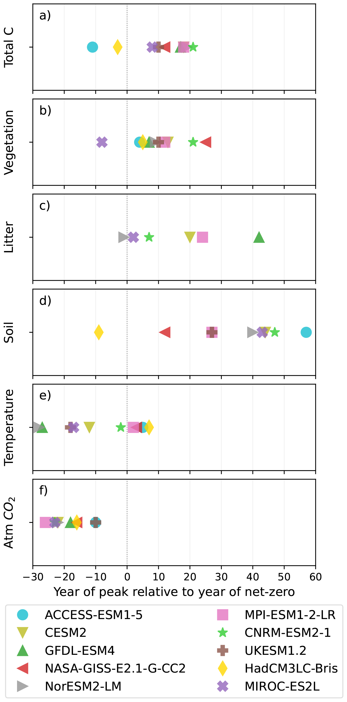
Figure 6 Year of peak relative to year of net-zero. Each panel shows the year at which that variable reaches its maximum value relative to the year in which emissions reach zero in the esm-flat10-cdr experiment. Each of the ESMs participating in flat10MIP is represented by one symbol. Rows show (from top) total carbon, vegetation carbon, litter carbon, soil carbon, globally averaged near surface temperature, and globally averaged atmospheric CO₂ concentration.

3.5 Unresolved structural and parametric uncertainty

We investigated how process representation impacted terrestrial carbon cycle behavior across these 10 ESMs by examining carbon stock changes (Fig. 3, Tables A1, A2). ESMs differ in their structural representation of key processes, including nutrient limitation, dynamic vegetation and biogeography, the complexity of soil carbon representation, and representation of dynamic fires (Table 1). None of the structural differences that we investigated correlate with carbon cycle behavior across this ESM ensemble (Figs. A7, A8, A9, A10). As an example, it is reasonable to assume that representation of nutrient dynamics and nutrient limitation would lead to a moderated increase in land carbon sink under very large cumulative emissions, yet ESMs with dynamic nutrients span the full range from the largest to the smallest land sink, as well as several in between the extremes (Figs. 3a, A7). We find the same lack of correspondence for interactive fire: fire is active in five of the ten ESMs (Table 1), yet these ESMs neither cluster together nor separate from the others in the magnitude or sign of their carbon stock changes (Figs. 3, A9). Regarding whether the spread is smaller among ESMs with more complex soil representations: the three depth-resolved ESMs (CESM2, NorESM2-LM, GFDL-ESM4) do not show tighter agreement than the single- or few-pool models; GFDL-ESM4 and NorESM2-LM sit at opposite ends of the initial soil carbon range despite both resolving soil by depth (Table A1, A10). However, only 10 ESMs are represented in flat10MIP, each with a single realized combination of processes and parameters. In addition to structural differences, parametric uncertainty can create a wide array of behavior within a single model (Booth et al., 2012; Kennedy et al., 2025; McNeall et al., 2024). These two factors confound the problem, leading to a multitude of possible differences across the 10 ESMs. In short, we find it likely that far too many aspects vary across these models for us to find a robust attribution of model behavior to process inclusion. Systematic investigations of the role of specific processes and parametric uncertainty within ESM simulations through controlled experimentation are needed to isolate the importance of processes and process representation in controlling terrestrial carbon cycle behavior.

The spread in carbon cycling across models has implications for global scale climate metrics. The first set of flat10MIP simulations (Sanderson et al., 2025) have a range of TCRE across the ensemble of 1.32 K per 1000 Pg C, with TCRE values across ESMs ranging from 1.18 to 2.50. However, the multi-model ensemble may underestimate the potential range of land carbon cycle uncertainty, due to lack of process understanding and parametric uncertainty. Slight variations in land parameter assumptions in a perturbed parameter ensemble that varied assumptions only about land processes from Booth et al. (2012) show a range of TCRE of 2.2 K per 1000 Pg C within a single model, with TCRE values from 1.57 to 3.77. Thus a single ESM has the potential to generate a wide range of TCRE, and possibly ZEC as well, due to different rates of carbon sinks alone, and this structural and parametric uncertainty has not yet been sampled either within or across ESMs.

4 Conclusions and Implications

ESMs participating in flat10MIP have a wide range of magnitude of pre-industrial carbon stocks. They additionally disagree on the zonal distribution of carbon as well as the partitioning between vegetation and soil carbon. ESMs in this study have been used in emissions-driven simulations, which by definition prognostically calculate atmospheric CO₂ as an emergent balance between sources (of which human emissions are specified) and sinks calculated within the ESMs. Given that many of these ESMs have been used to simulate the historical period, these ESMs can be compared against observed historical trajectories of atmospheric CO₂ (Hajima et al., 2025). Observations of atmospheric CO₂ carbon stocks, made through measurements of atmospheric CO₂ mixing ratio, are far more precise than observational estimates for either land or ocean stocks, and particularly for the zonal distribution of such stocks. The considerable uncertainty associated with the best estimates of land and ocean carbon stocks contribute to the lack of convergence on pre-industrial carbon stocks across ESMs.

Although the wide range of simulated pre-industrial carbon stocks across the ESMs we analyze here are therefore not a surprise, this spread still has implications for the subsequent behavior of land carbon sinks. Recent assessments of the offline properties of the present set of global land surface schemes indicates that large ranges in predicted soil and vegetation carbon remain (Friedlingstein et al., 2026). Refinements in the simulation of vegetation growth processes that allow more detailed constraints on vegetation growth rate, turnover and structure via consideration of vegetation demography, may help narrow the range of model predictions moving forwards.

Our findings here highlight that tropical carbon is most likely to be both gained and subsequently lost under positive, zero, declining, and negative emissions. This creates possible headwinds for carbon dioxide removal through afforestation and reforestation, the majority of which is projected to be implemented in low latitudes (Griscom et al., 2017; Cook-Patton et al., 2020; Mo et al., 2023). The esm-flat10-cdr simulations impose the magnitude of the carbon dioxide removal as a boundary condition of the emissions-driven scenario through a negative emissions flux – they do not directly model the processes driving carbon dioxide removal some of which could have additional climate impacts due to physical changes to the land surface (i.e. Swann et al., 2012; King et al., 2024). Similarly, esm-flat10-zec simulations represent either zero or net-zero emissions, the latter of which implicitly includes carbon dioxide removal. In reality, our ability to remove CO₂ from the atmosphere, in particular through reforestation or afforestation, is likely to be negatively affected by the same adverse conditions for carbon storage that provoke the loss in tropical carbon stocks in these scenarios.

Timescales associated with vegetation carbon, as measured by the timing of peak vegetation carbon relative to the time of net-zero emission under the esm-flat10-cdr scenario, are relatively consistent across ESMs and across latitudes (Figs. 6, A6). Soil carbon timescales, on the other hand, vary widely across ESMs at all latitudes. The disagreement between both soil initial states and soil response timescales highlights greater structural uncertainty associated with soil carbon pools, as well as the challenge associated with assessing the behavior of a slowly evolving pool.

The wide variation across ESMs in soil carbon responses, which set the longest timescale of terrestrial carbon cycle response, has important implications for the role of terrestrial carbon cycle uncertainties for influencing ZEC. ZEC is an emergent property of the Earth system that captures the decadal- to century-timescale adjustment of temperature following net zero emissions. It emerges as a balance between the slowing of ocean heat uptake balanced by reductions in radiative forcing from CO₂ as land and ocean sinks draw carbon out of the atmosphere (Jones et al., 2019; MacDougall et al., 2020; Palazzo Corner et al., 2023). Timescale responses longer than decades are particularly important in setting ZEC, and thus the response of soil carbon pools on land, as well as ocean carbon uptake, are likely to be more important for ZEC than vegetation carbon timescales. Given the lack of agreement across the ESMs analyzed here on the timing of soil carbon response, constraining ZEC from ESM behavior remains a challenge, and highlights the urgent need to better understand and simulate soil carbon processes.

Appendix A: Terrestrial carbon cycle representation in each ESM

Below we provide an overview of relevant aspects of the representation of terrestrial carbon cycling in each ESM analyzed here. Additional simulation details can be found in Appendix A1 of Sanderson et al. (2025).

A1 ACCESS-ESM1-5

ACCESS-ESM1-5 (Ziehn et al., 2020) uses the CABLE land surface model (Kowalczyk et al., 2013) with biogeochemistry implemented through the CASA-CNP module, which includes the carbon cycle with added nitrogen and phosphorus cycles (Wang et al., 2010). The CABLE configuration in ACCESS-ESM1-5 uses 10 vegetation land cover types and a prognostic leaf area index based on the size of the leaf carbon pool and the specific leaf area. The flow of carbon and nutrients is simulated between three plant biomass pools (leaf, wood, root), three litter pools (metabolic, structural, coarse woody debris) and three organic soil pools (microbial, slow, passive) plus additional nitrogen (inorganic) and phosphorus (labile, sorbed, strongly sorbed) soil pools. All simulations have been run with nitrogen and phosphorus limitation enabled.

A2 CESM2

The terrestrial carbon cycle in CESM2 (Danabasoglu et al., 2020) used v5 of the Community Land Model (CLM5, Lawrence et al., 2019), a big-leaf representation of coupled carbon and nitrogen cycling, which includes representation of permafrost, crops, methane cycling, and urban, lake, glaciated and bare ground land cover types (land use is held fixed at pre-industrial conditions for flat10MIP experiments). CLM5 contains a hydrodynamic representations of plant drought stress and soil moisture uptake (Kennedy et al., 2019), as well as representations of shifts in plant nutrient acquisition between active uptake and fixation (Fisher et al., 2019). Temperature acclimation of both photosynthesis and respiration is represented (Lombardozzi et al., 2015). The responses of carbon cycling to inter-annual variability in moisture availability are lower, and the response to CO₂ fertilization greater than in the previous version of the CLM (Wieder et al., 2019).

A3 GFDL-ESM4

The NOAA Geophysical Fluid Dynamics Laboratory (GFDL) ESM4 model (Dunne et al., 2020) includes the GFDL Land Model version 4.1 (LM4.1, Shevliakova et al., 2024) dynamic land vegetation component. Land hydrology and ecosystem dynamics are represented on the same 1° grid as the GFDL Atmospheric Model version 4.1 (AM4.1, Horowitz et al., 2020) atmospheric component, which includes interactive aerosols and chemistry.

LM4.1 represents sub-grid scale heterogeneity of the land surface via a mosaic approach that divides each land grid cell into multiple tiles, each representing unique physical and biological properties. Within each tile, LM4.1 represents multiple vegetation cohorts per layer, of different ages and vegetation types, with cohort-specific energy balance and intercepted water/snow. Radiation treatment includes multistory canopy dynamics, with transpiration and stomatal conductance based on Wolf et al. (2016). Prognostic vegetation distribution dynamics are represented by a fully consistent explicit treatment of ecosystem demography, multi-layer vegetation canopy, and land surface processes, and include age-height structured vegetation competition for light – the Perfect Plasticity Approximation (PPA, Purves and Pacala, 2008; Weng et al., 2015). LM4.1 includes 6 plant functional types (PFTs) in representing C₃ grass, C₄ grass, tropical trees, temperate deciduous trees, and cold evergreen trees. 6 live carbon pools in LM4.1 represent leaves, fine roots, heartwood, sapwood, seeds, and non-structural carbon (i.e., sugars). Carbon gain is allocated daily to leaves, fine roots, sapwood, seeds, and non-structural carbon pools according to the tree-grass allometric relationship (Martínez Cano et al., 2020; Weng et al., 2015).

Soil carbon dynamics and biogeochemistry are represented by the Carbon, Organisms, Rhizosphere, and Protection in the Soil Environment (CORPSE, Sulman et al., 2014, 2019) model. Litter is divided into leaf and coarse-wood categories, and into fast- and slow-timescale partitions. Each of the 20 vertical soil levels represents separate fast and slow soil carbon pools, along with two carbon storage pools associated with soil microbes and microbial products. LM4.1 includes the FINAL v2 fire model (Rabin et al., 2015, 2018; Ward et al., 2018) representing daily fire, including both multi-day and crown fires. The LM4.1 component in GFDL-ESM4 does not include an interactive nitrogen cycle and does not formally represent long-term permafrost cycling. Instead, a 500-year maximum soil lifetime is included to prevent accumulation of recalcitrant material under cold, dry conditions and to achieve land carbon equilibration.

A4 NASA-GISS-E2.1-G-CC2

The NASA Goddard Institute for Space Studies ESM ModelE, version NASA-GISS-E2.1-G-CC2 (Romanou et al., 2026) has a coupled carbon cycle (Ito et al., 2020b) that uses the Ent Terrestrial Biosphere Model (Ent TBM, Kim et al., 2015) for land carbon dynamics and an updated version of the NASA Ocean Biogeochemistry Model (NOBM, Romanou et al., 2013, 2014), coupled through atmospheric CO₂ tracers (Romanou et al., 2013, 2014). The Ent TBM simulates 12 plant functional tyeps (PFTs), including one crop type (land use is held fixed at pre-industrial conditions for flat10MIP experiments). Soil biogeochemistry is the CASA' model (Randerson et al., 2009; Doney et al., 2006), with 9 soil carbon pools and updated soil moisture sensitivity (Kim et al., 2015). The 9 soil carbon pools are simulated in one soil layer averaging the upper 30 cm of soil microclimate. Photosynthetic uptake of carbon is stored in a labile non-structural carbohydrate pool, which is withdrawn for autotrophic respiration, seasonal leaf growth, allocation to a reproductive pool, and stem growth, as well as replenished through retranslocation from senescing foliage. The Ent TBM does not currently include nitrogen dynamics, land use state transition, wood harvest, deforestation, fire, or community dynamics or mortality and establishment.

For this study, the Ent TBM was run in a configuration with “biophysics-only” dynamics, in which vegetation boundary conditions (cover fraction, canopy heights, leaf area index) were prescribed from a satellite-derived observational data set, as described in Ito et al. (2020b). Crop cover was prescribed at constant 1850 conditions from the Land Use Harmonization version 2 (LUH2) data set (Hurtt et al., 2020), using the updated years from the Global Carbon Budget project (Friedlingstein et al., 2025b), combining all LUH2 crop cover types into one Ent C₃ crop type. In the biophysics mode with fixed vegetation structure, the prognostic land carbon pools are the plant labile carbon and soil carbon pools. The labile carbon pool balance is subject to the same fluxes of respiration and allocation/retranslocation, but not reproduction, and the carbon that would be allocated to stem growth is instead dropped as litterfall to the soil. To prevent carbon deficits, at low labile carbon balances, autotrophic respiration is reduced or turned off rather than causing mortality, until the labile carbon pool replenishes. Therefore, enhanced carbon uptake due to the CO₂ fertilization effect is expressed in the biophysics-only mode as increased litterfall. The enhanced litterfall is not inconsistent with the increased turnover that can happen with CO₂ fertilization without increases in biomass in mature ecosystems, and with increased soil carbon storage, as observed in the tropics by (Bar-On et al., 2025).

A5 NorESM2-LM

The land carbon cycle in NorESM2-LM (Seland et al., 2020) is based on the Community Land Model 5 (CLM5, Lawrence et al., 2019). As such, the land component is very similar, but not identical, to the land component of CESM2. The main differences arise in soil carbon. NorESM2-LM simulates the carbon and nitrogen cycles, including natural vegetation, litter, and soil carbon pools. In addition to temperature and precipitation, the land CO₂ fluxes are also influenced by atmospheric CO₂ concentrations and atmospheric nitrogen deposition. The NorESM2-LM model was not spun-up long enough prior to starting the flat10 simulation, leading to a considerable preindustrial drift in the land carbon pools. We have therefore drift-corrected all changes in land carbon stocks presented here by estimating the trend at the end of the pre-industrial period in each gridcell and then removing the trend over all time series.

A6 MPI-ESM1-2-LR

The land surface model of MPI-ESM1-2-LR, JSBACH3.20, includes components to describe the dynamics of terrestrial vegetation and the carbon cycle in interaction with the global climate (Mauritsen et al., 2019). Terrestrial vegetation in JSBACH includes a competition scheme for vegetation dynamics based on the productivity of woody and herbaceous plants (Brovkin et al., 2009). Vegetation dynamics are influenced by wildfires and anthropogenic fires simulated by the SPITFIRE model, which provides the area burned and carbon emissions to the atmosphere (Lasslop et al., 2014). The soil carbon model YASSO simulates the dynamics of four fast soil carbon pools, which differ for leaf and wood litter types, and one slow humus pool. YASSO simulates plausible soil density patterns with relative maxima in tropical and boreal forests, and the distribution is comparable to observations (Mauritsen et al., 2019). JSBACH3.20 did not include permafrost carbon, and the maximum soil carbon storage at high northern latitudes is not well captured by the model. Nitrogen and carbon pools are coupled based on CO₂-induced nitrogen limitation (Goll et al., 2017).

A7 CNRM-ESM2-1

This study analyzes model outputs of CNRM-ESM2-2 (Bossert et al., 2025). Compared to its previous version (CNRM-ESM2-1, Séférian et al., 2019), CNRM-ESM2-2 offers an improved representation of the global carbon cycle, and of several Earth system interactions (aerosols-light, biophysics, etc.).

The SURFEX v8.0 platform (Masson et al., 2013) is the surface component of CNRM-ESM2-1. It simulates surface state variables and fluxes at the surface-atmosphere interface, using the same grid and time step as the atmosphere model. ISBA-CTRIP represents the land carbon cycle by simulating plant physiology, carbon allocation, and soil carbon cycling (Delire et al., 2020). It includes modules for wildfires and dissolved organic carbon transport to the ocean. Vegetation is modeled with 4–6 carbon pools depending on plant type, and 16 vegetation types are distinguished. Photosynthesis is represented by a semi-empirical model with a 10-layer radiative transfer scheme, while leaf phenology is driven by carbon balance. Soil carbon dynamics follow the CENTURY model (Parton et al., 1988), with four litter and six soil carbon pools releasing CO₂ through decomposition. Further details are provided in Decharme et al. (2019) and Delire et al. (2020).

A8 HadCM3LC-Bris

HadCM3LC-Bris is based on the HadCM3 climate model (Gordon et al., 2000), adapted for use with an interactive carbon cycle by adopting lower ocean resolution (Cox, 2001) and subsequently modified for use at University of Bristol (Valdes et al., 2017). The land carbon cycle is based on the MOSES-2 land surface model (Essery et al., 2003), with dynamic vegetation which simulates phenology, growth and competition of five plant functional types (broad-leaved and needle-leaved trees, C₃ and C₄ grasses and shrubs). Soil carbon is represented in a single pool, with an exponential “q10” dependence of decomposition on soil temperature (e.g. Lloyd and Taylor, 1994).

A9 UKESM1.2

UKESM1.2 is based on UKESM1.1 (Mulcahy et al., 2023) with the addition of interactive ice sheets over Greenland and Antarctica provided by the BISICLES model (Smith et al., 2021). The atmosphere model within UKESM1.2 is vn12.1 of the Met Office Unified Model, which is coupled to the NEMO ocean model. The land and ocean carbon cycle components of UKESM1.2 are essentially unchanged from UKESM1-0-LL (Sellar et al., 2019). The land surface scheme consists of the JULES land surface model (Clark et al., 2011; Harper et al., 2016), which includes 13 natural and 4 agricultural plant functional types, whose spatial distribution is determined by height-based competition via the TRIFFID dynamic vegetation model (Cox, 2001, land use is held fixed at pre-industrial conditions for flat10MIP experiments). Net primary productivity is limited by nitrogen availability (Wiltshire et al., 2021).

A10 MIROC-ES2L

The MIROC Earth system version 2 for long-term simulations (MIROC-ES2L; Hajima et al., 2020) is a model that was extensively used for the Coupled Model Intercomparison Project phase 6. The version used in this study is the same as that used for CMIP6 except for several bug fixes, and the spin-up was extended before performing the flat10-experiment. The land biogeochemical component is VISIT (Ito and Inatomi, 2012), which is interactively coupled to the land surface physics model (MATSIRO; Takata et al., 2003). The terrestrial biogeochemical component covers major processes relevant to the global carbon cycle, with vegetation (leaf, stem, and root), litter (leaf, stem, and root), and humus (active, intermediate, and passive) pools, under a static vegetation distribution. The nitrogen cycle is simulated with N pools consisting of vegetation (canopy and structural), organic soil (litter, humus, and microbe), and inorganic nitrogen (ammonium and nitrate).

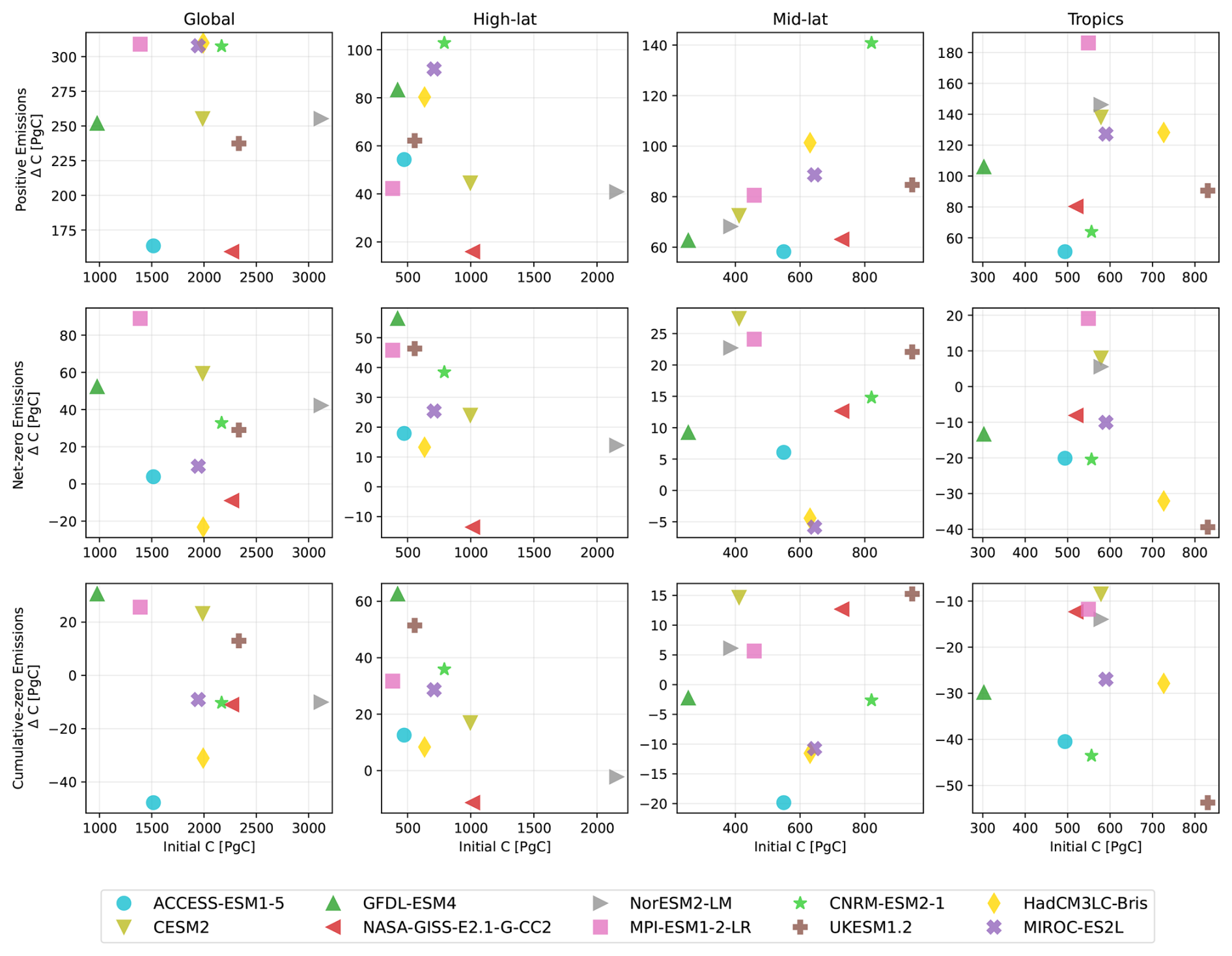
Figure A1 Change in carbon during different phases as a function of initial carbon. Change in carbon in units of Pg C for during the positive emissions phase (top), net-zero phase (middle), and cumulative-zero phase (bottom) plotted against the initial carbon in units of Pg C. Columns show results averaged over land for different regions including global average (left column), high-latitudes (second column), mid-latitudes (third column), and tropics (fourth column). Symbols and colors denote different ESMs.

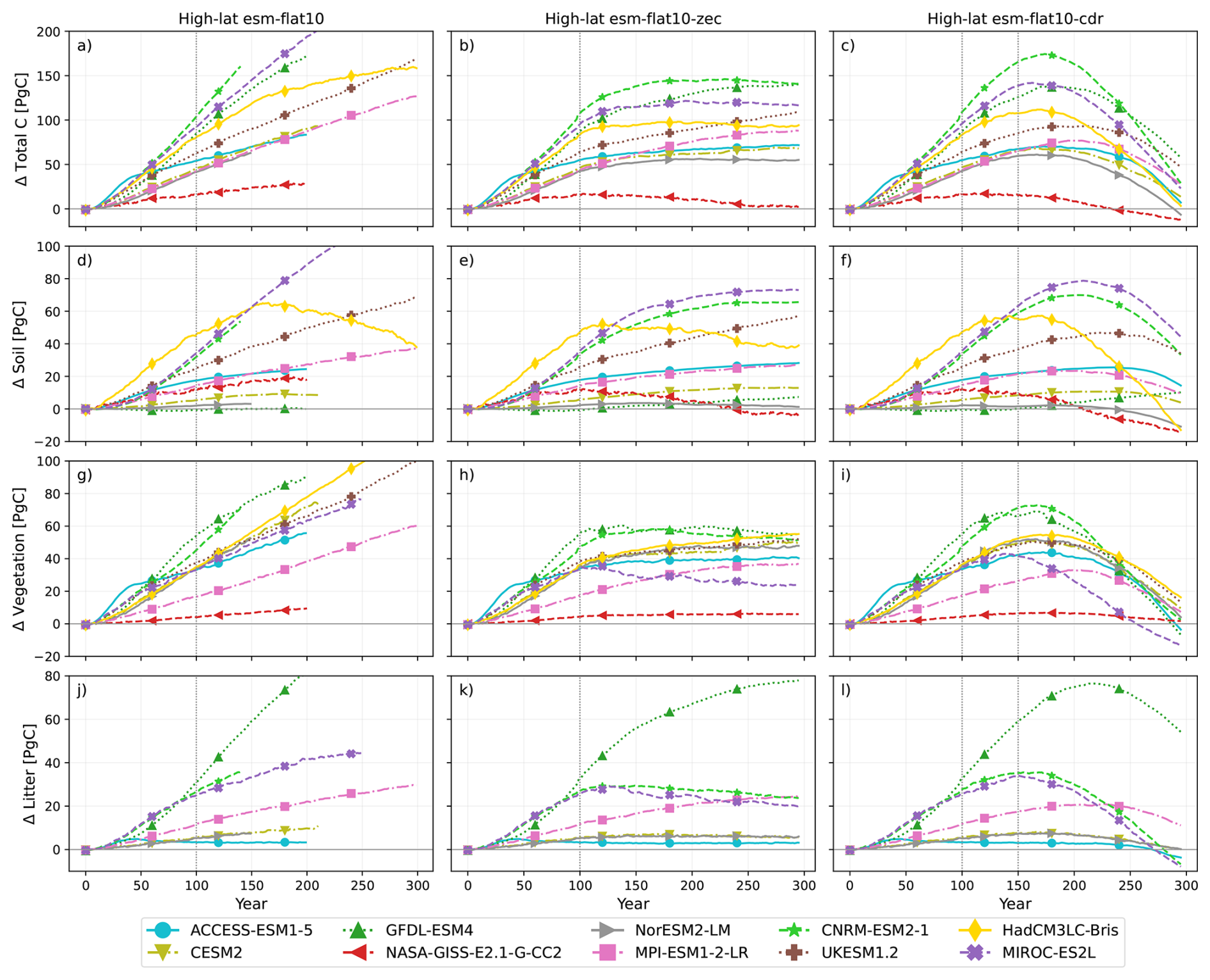
Figure A2 Timeseries of carbon pools for high-latitudes. Time series of change in carbon stocks in high-latitudes in each of the ESMs participating in flat10MIP in units of Pg C with total carbon in the top row, soil carbon in the second row, and vegetation carbon in the third row, and litter carbon in the fourth row (not all ESMs report litter). Columns show each of the three experiments: esm-flat10 (left), esm-flat10-zec (middle), and esm-flat10-cdr (right). Each colored line represents one ESM. The vertical dashed lines indicate the year of 1000 Pg C of cumulative emissions, which corresponds to the year of net-zero emissions in esm-flat10-zec, as well as year 150 in the right hand column which is the year of net-zero emissions in esm-flat10-cdr.

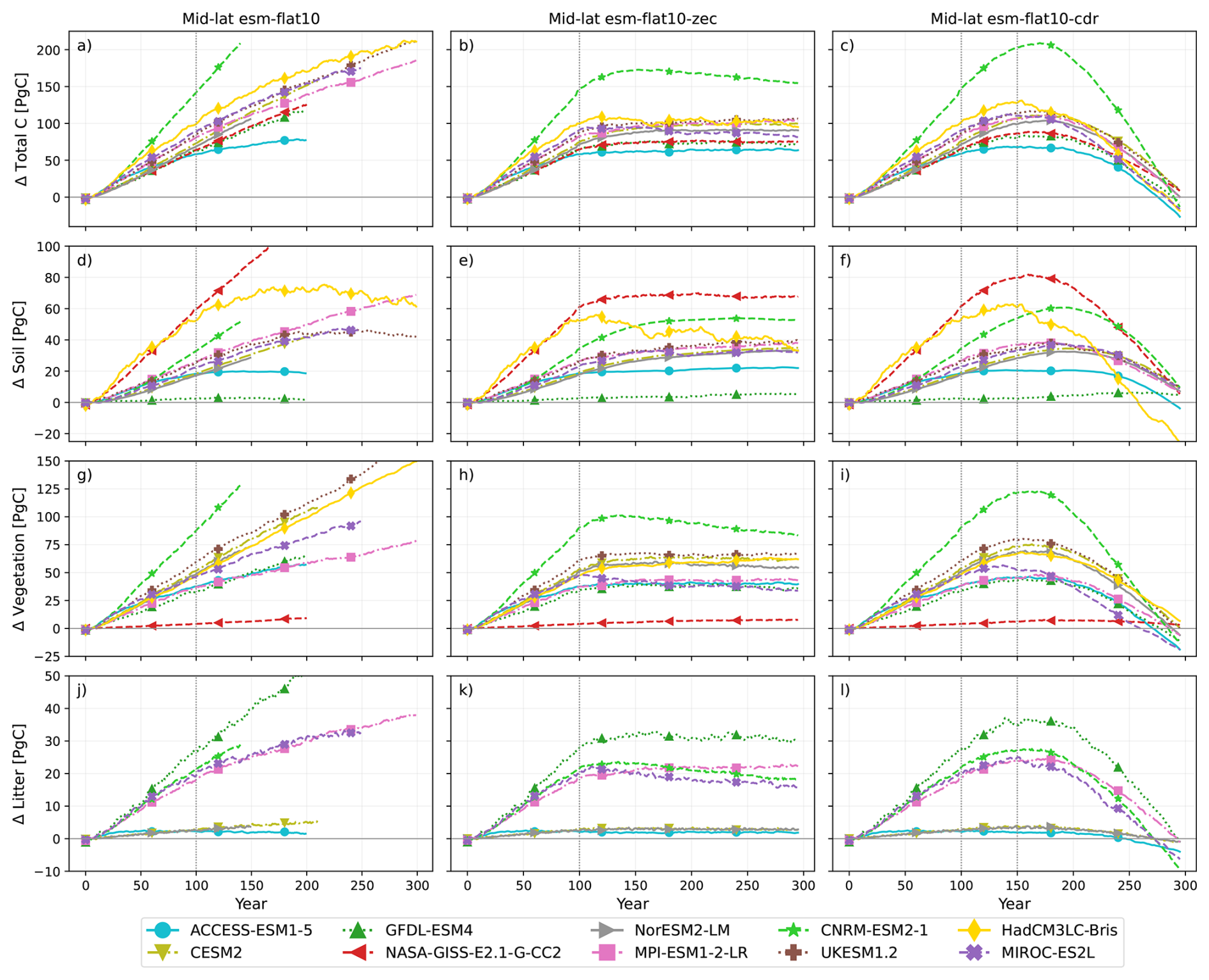
Figure A3 Timeseries of carbon pools for mid-latitudes. Time series of change in carbon stocks in mid-latitudes in each of the ESMs participating in flat10MIP in units of Pg C with total carbon in the top row, soil carbon in the second row, and vegetation carbon in the third row, and litter carbon in the fourth row (not all ESMs report litter). Columns show each of the three experiments: esm-flat10 (left), esm-flat10-zec (middle), and esm-flat10-cdr (right). Each colored line represents one ESM. The vertical dashed lines indicate the year of 1000 Pg C of cumulative emissions, which corresponds to the year of net-zero emissions in esm-flat10-zec, as well as year 150 in the right hand column which is the year of net-zero emissions in esm-flat10-cdr.

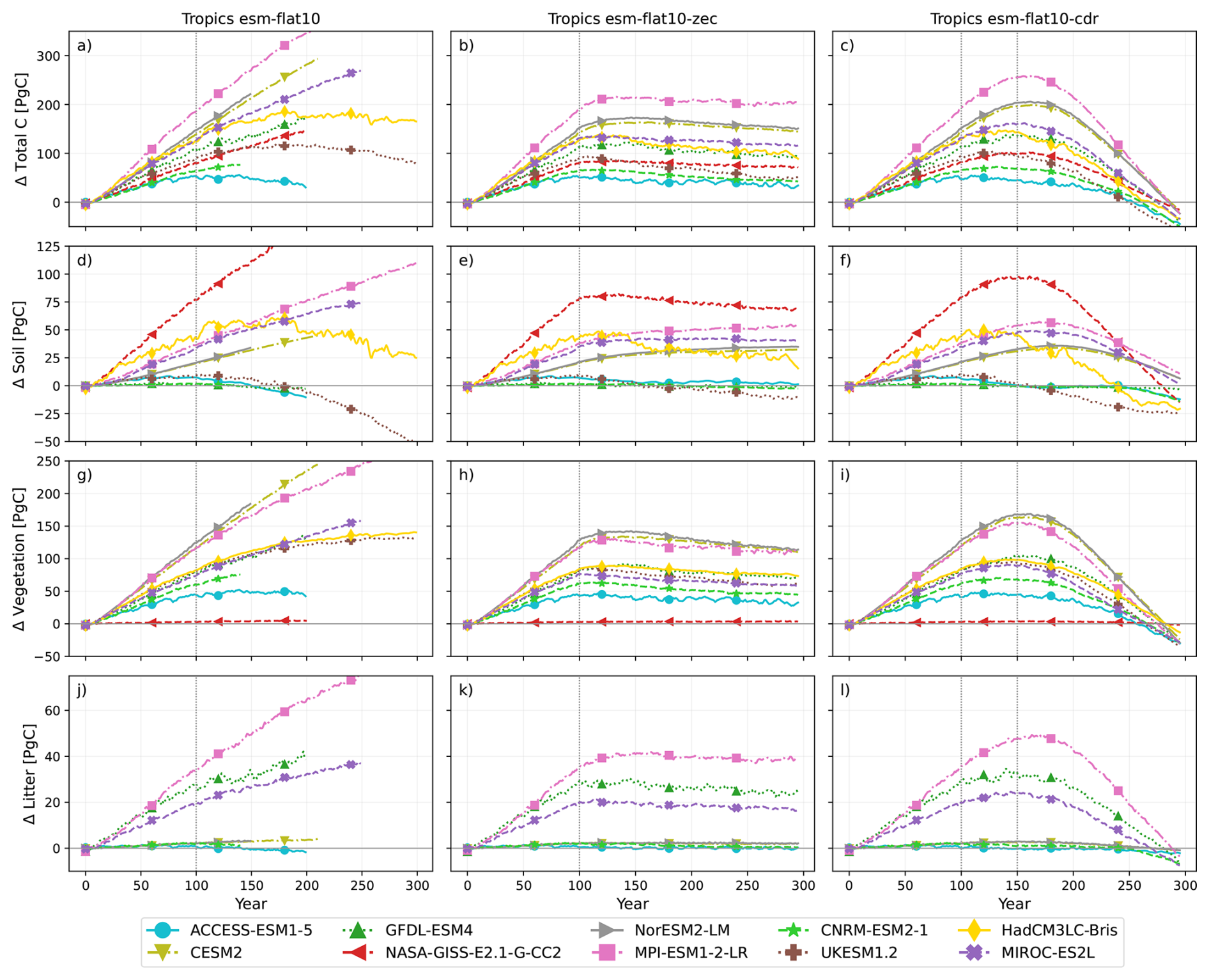
Figure A4 Timeseries of carbon pools for tropical latitudes. Time series of change in carbon stocks in tropical latitudes in each of the ESMs participating in flat10MIP in units of Pg C with total carbon in the top row, soil carbon in the second row, and vegetation carbon in the third row, and litter carbon in the fourth row (not all ESMs report litter). Columns show each of the three experiments: esm-flat10 (left), esm-flat10-zec (middle), and esm-flat10-cdr (right). Each colored line represents one ESM. The vertical dashed lines indicate the year of 1000 Pg C of cumulative emissions, which corresponds to the year of net-zero emissions in esm-flat10-zec, as well as year 150 in the right hand column which is the year of net-zero emissions in esm-flat10-cdr.

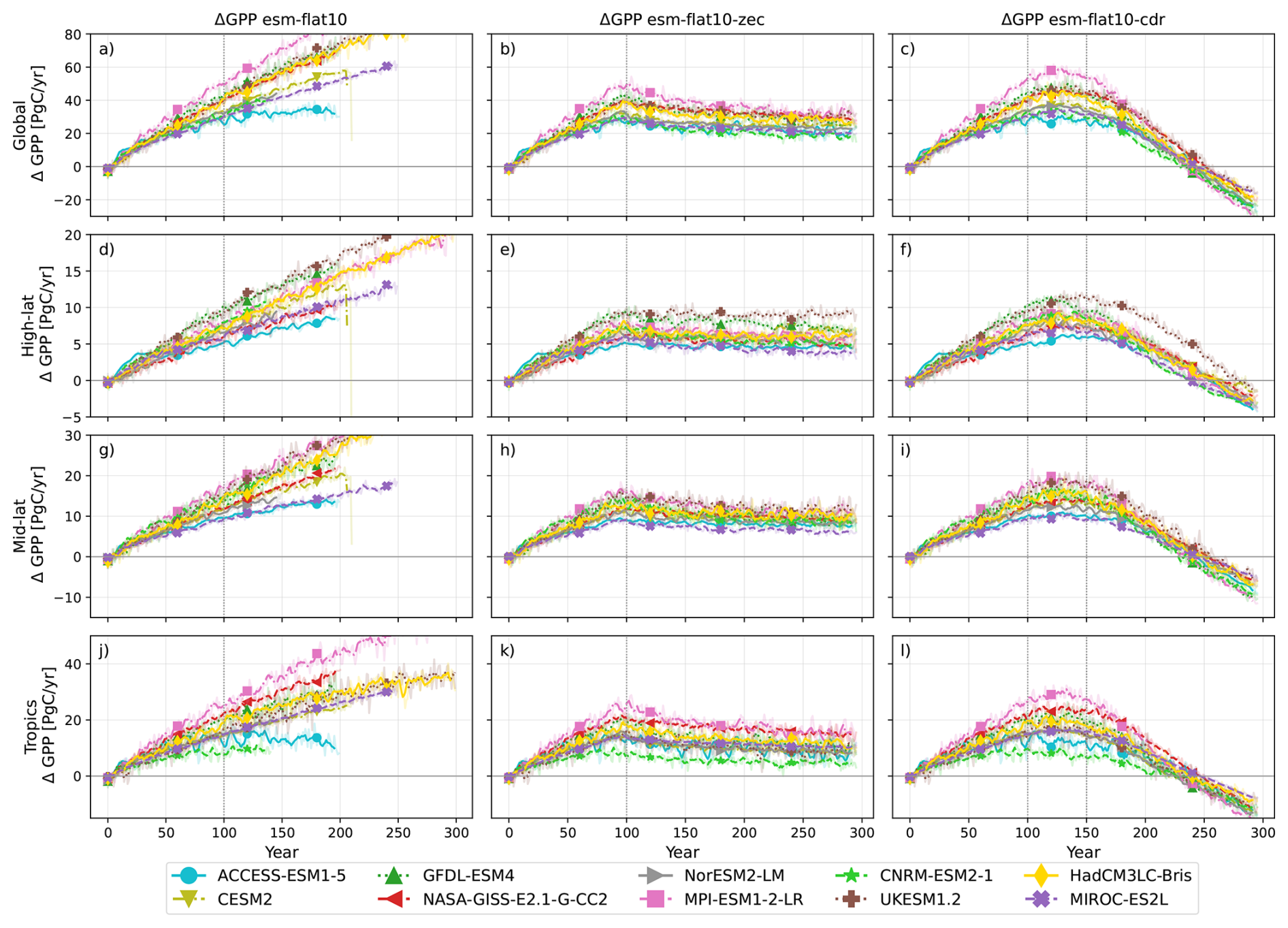
Figure A5 Timeseries of GPP for different latitudes. Time series of change in GPP at different latitudes in each of the ESMs participating in flat10MIP in units of Pg C with the global average in the top row, high-latitude average in the second row, mid-latitude average in the third row, and tropical average in the bottom row. Columns show each of the three experiments: esm-flat10 (left), esm-flat10-zec (middle), and esm-flat10-cdr (right). Each colored line represents one ESM. The vertical dashed lines indicate the year of 1000 Pg C of cumulative emissions, which corresponds to the year of net-zero emissions in esm-flat10-zec, as well as year 150 in the right hand column which is the year of net-zero emissions in esm-flat10-cdr. Light shaded lines show the full interannual variability and soild colored lines have been smoothed with a 5 year running mean.

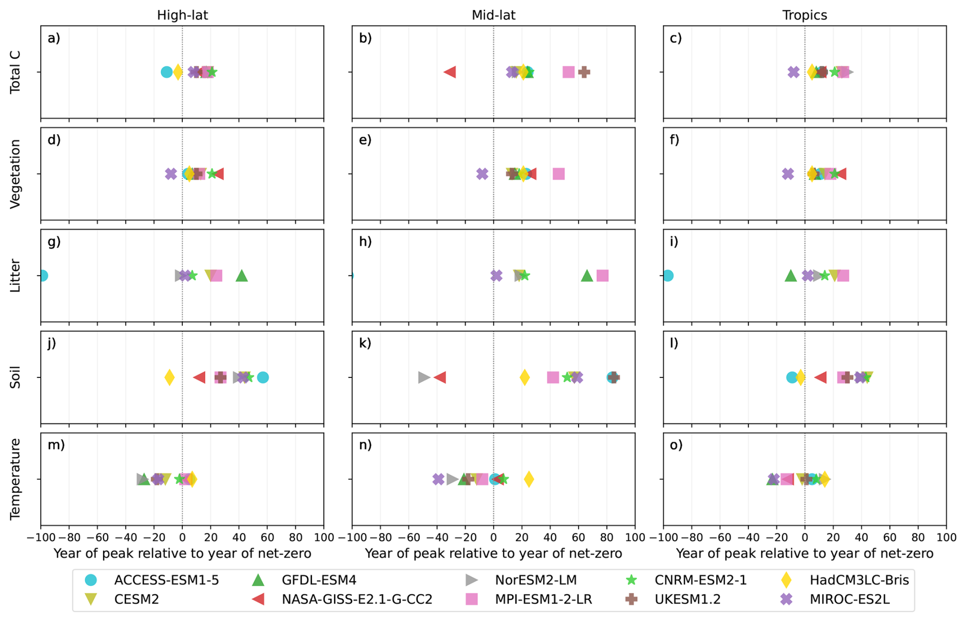
Figure A6 Year of peak relative to year of net-zero for different latitude bands. Each panel shows the year at which that variable reaches its maximum value relative to the year in which emissions reach zero in the esm-flat10-cdr experiment. Each of the ESMs participating in flat10MIP is represented by one symbol. Rows (from top) show total carbon, vegetation carbon, litter carbon, soil carbon, near surface temperature, and globally averaged atmospheric CO₂ concentration. Columns (from left) show global land average, high-latitude land average, mid-latitude land average, and tropical land average.

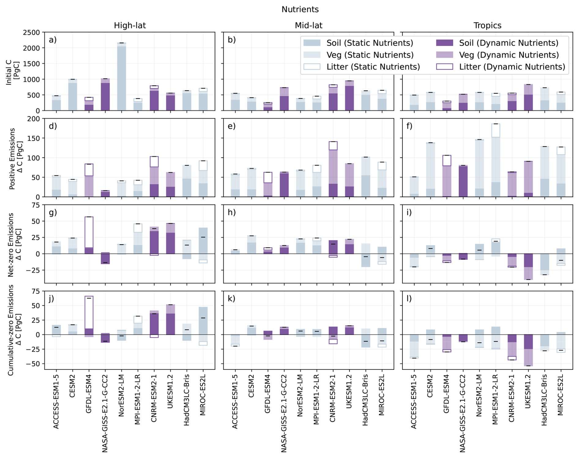
Figure A7 Carbon and Δcarbon at different latitudes colored by nutrient dynamics. Bar graph showing initial carbon stocks (first row), and change in carbon stocks after positive emissions (second row), after net-zero emissions (third row), and after negative emissions (fourth row) in each of the ESMs participating in flat10MIP. Each column shows the initial stock or change in C for soil carbon (solid dark color), vegetation carbon (lighter color), and litter (white with outline) high-latitudes (>50°) in the left column, mid-latitude regions (>20° and <50°) in the middle column, and tropical regions (<20°) in the right column. Positive values are plotted above the zero line and negative values are plotted below the zero line. The total C (sum of all bars) is indicated with a black bar. This figure shows the same data as main text Fig. 2, except that here colors indicate models with either dynamic or static representation of nutrient limitation.

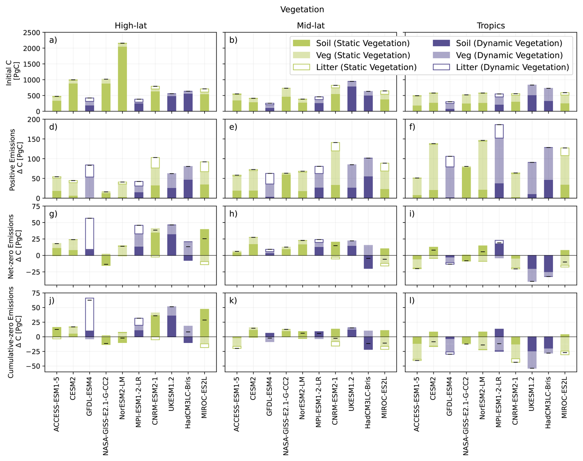
Figure A8 Carbon and Δcarbon at different latitudes colored by dynamic vegetation and biogeography. As in Fig. A7, with colors that indicate models with either dynamic or static representation of vegetation dynamics and biogeography.

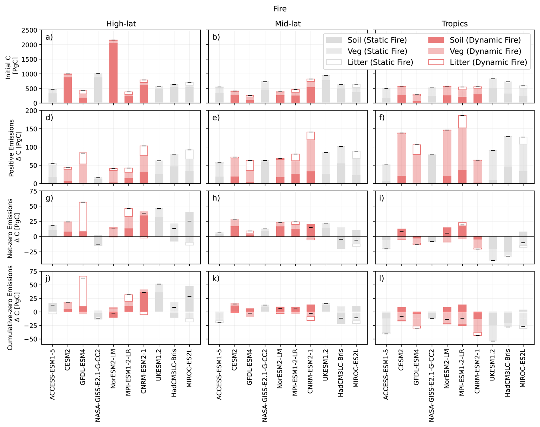
Figure A9 Carbon and Δcarbon at different latitudes colored by dynamic fires. As in Fig. A7, with colors that indicate models with either dynamic or static representation of dynamic fires.

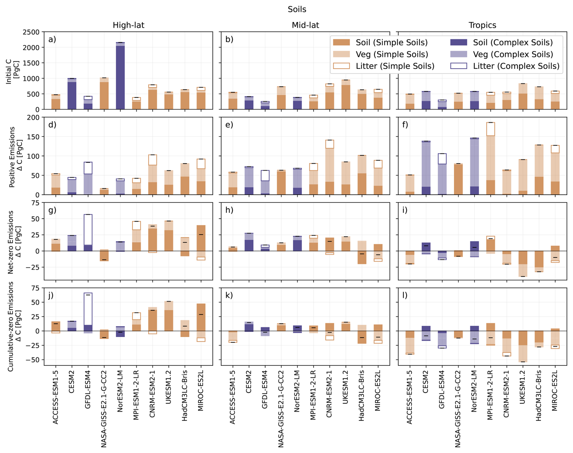
Figure A10 Carbon and Δcarbon at different latitudes colored by complexity of soil carbon pools. As in Fig. A7, with colors that indicate models with either dynamic or static representation of complexity of soil carbon pools, where complex denotes depth resolved soil carbon pools.

Table A1 Initial Carbon content and change under different emissions by pool. Carbon stocks and changes in stocks are in units of Pg C.

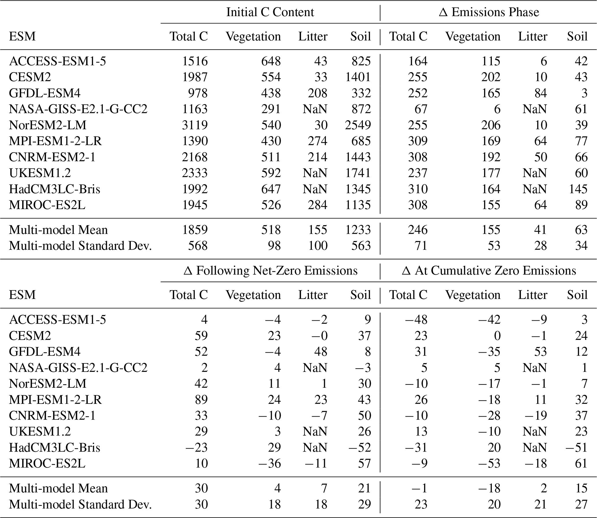
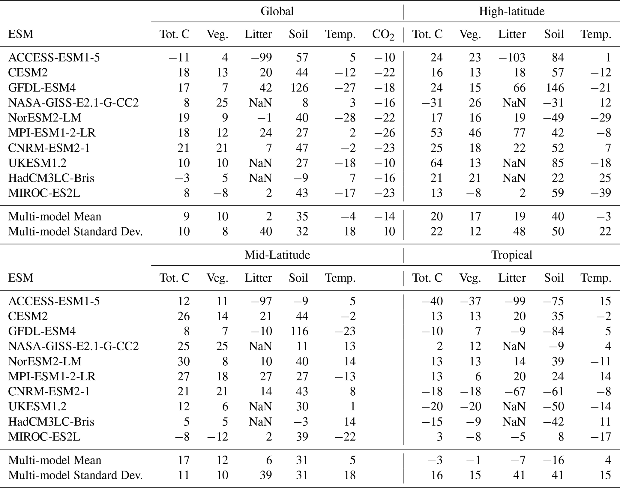
Table A2 Initial Carbon content and change under different emissions by latitude. Carbon stocks and changes in stocks are in units of Pg C.

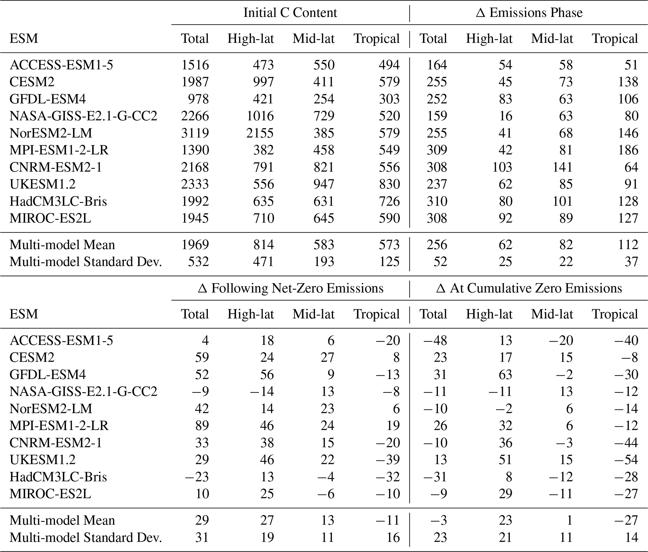
Table A3 Lead or lag of peak relative to year of net-zero emissions for each latitude band. Each column represents the lead or lag for a given variable in years.