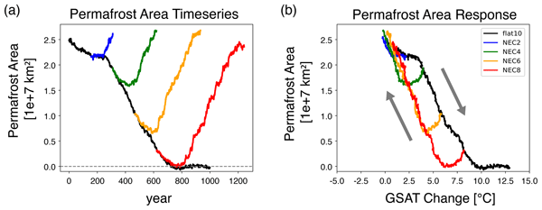
Hysteresis and irreversibility in permafrost physical response to increase and decrease of CO₂ emissions

Boreal permafrost over the Northern Hemisphere high latitudes, defined as areas where the ground temperature is below 0 °C for two or more years, stores more than twice as much carbon as the atmosphere. Therefore, thawing of the permafrost, a tipping element, due to global warming may lead to additional carbon emissions and accelerate the warming. To investigate the permafrost response to increase and decrease of CO₂ emissions, we conducted a series of numerical experiments using an emission-driven Earth System Model, MIROC-ES2L, and adopting idealized overshooting scenarios in which a prescribed CO₂ emission of 10 PgC yr⁻¹ is given until the global warming level reaches different values between 2 and 8 °C followed by the negative emission until the cumulative emission becomes zero.

We found that the response of permafrost area to surface warming and cooling is reversible but has hysteresis for all the emission scenarios. Furthermore, the permafrost property such as the ratio of frozen to liquid water was shown to have irreversibility in the deep soil layer; part of the frozen area in the initial condition was replaced by a mixed water-ice area in the final state despite ground temperature returning almost to the initial condition. Sensitivity experiments reveal that the hysteresis and irreversibility are attributed to the delay of the soil freezing and melting associated with the soil heat conductivity and specific heat of water phase change. This result indicates that once permafrost thaws with warming it will continue for decades after warming diminishes and the delay in the permafrost recovery is larger at global warming levels greater than 2 °C. An offline calculation shows that the additional CO₂ emission during the permafrost hysteresis cycle accounts for about 0.6 %–41 % of the cumulative carbon emission released from thawed permafrost in flat10 and NEC experiments.

1 Introduction

Global warming due to anthropogenic carbon dioxide (CO₂) emissions is ongoing and the global-mean surface air temperature (GSAT) has increased by 1.1 °C since the preindustrial era (Canadell and Monteiro, 2021). Many efforts have so far been made to clarify impacts of increasing anthropogenic CO₂ emissions on the Earth system using Earth System Models (ESMs) (Sanderson et al., 2024).

Permafrost is defined as an area where soil temperature remains below 0 °C for more than two consecutive years. Northern Hemisphere (NH) permafrost region, spreading approximately 21 million km² over northern Eurasia, Canada, and Himalayas (Obu, 2021), contain about twice as much carbon as the atmosphere and three times as much as land plants (Schuur et al., 2008; Ping et al., 2008; Tarnocai et al., 2009; Hugelius et al., 2014; Yokohata et al., 2020a). As permafrost thaws with warming of land surface, carbon in the soil is released to the atmosphere as greenhouse gases (GHGs) in the form of CO₂ and methane (CH₄) (Schuur et al., 2015; Burke et al., 2017; Schuur et al., 2022; Hugelius et al., 2024). These GHG emissions will lead to further warming and therefore the permafrost thaw can trigger positive carbon-climate feedback (Lenton, 2012; Schaefer et al., 2014; Schuur et al., 2015; Burke et al., 2018). While the amount of carbon released from thawed permafrost is estimated to be about 18 (3–41, 5 %–95 % range) GtC per degree of global warming (Canadell and Monteiro, 2021; Winkelmann et al., 2023), there is a great deal of uncertainty in the estimate of additional GHGs released from permafrost thaw and their impact on climate due to factors such as the geographic characteristics of permafrost that make accurate estimation of soil carbon complex (Schuur et al., 2022; Park and Kug, 2022; Park et al., 2025). Schuur et al. (2022), who reviewed the permafrost–carbon cycle, argue that permafrost physical characteristics such as the ice content in the frozen ground are important for estimating the impact of permafrost thaw on the global carbon cycle. Park et al. (2025) estimated a permafrost carbon loss under overshoot scenarios but concluded that the amount of soil carbon emissions is still uncertain because the soil carbon content and the decomposition dynamics in deep soil layers are poorly understood. Therefore, investigating the response of permafrost to overshoot scenarios remains an important issue for accurately estimating the GHGs emissions from thawed permafrost.

The above processes are irreversible on the time scale of human society of, say, hundreds years because carbon stored in the permafrost during the last glacial period does not immediately return to the soil once it is released into the atmosphere even if the CO₂ concentrations is stabilized (Boucher et al., 2012). Soil organic carbon (SOC) in the permafrost is estimated to be 1100–1500 PgC globally, of which 1035 ± 150 PgC is in soils shallower than 3 m (Hugelius et al., 2014). The carbon-climate feedback associated with the permafrost thawing may occur even at a small global warming level because the thawing process will begin from near-surface soil layers. Much of the permafrost is expected to thaw on centennial timescales and is considered to exhibit tipping-element-like behavior which has a critical threshold at which small perturbations can cause qualitative changes in the state and development of a system (Luke and Cox, 2011; Hollesen et al., 2015; McKay et al., 2022; Brovkin et al., 2025).

Investigation of the physical response of permafrost to climate change is also critical to understand the permafrost behavior as one of key elements in the Earth system which may have hysteresis. It is important to understand how the permafrost will respond and to what extent its response may lag or differ depending on the path taken due to potential hysteresis in the case of successful climate mitigation efforts including the use of carbon dioxide removal techniques. Boucher et al. (2012) first showed the existence of hysteresis behaviour in the permafrost response to increase and decrease of the CO₂ concentration using an ESM. Their result suggests that once permafrost thaws due to global warming the effects will continue for some time, delaying the recovery of the permafrost during the climate cooling period. Eliseev et al. (2014) showed the mechanism of permafrost hysteresis using a simpler model called an Earth systems model of intermediate complexity, or EMIC. They found that hysteresis is related to the impact of phase transitions of soil water on apparent inertia of the system. However, further investigation of the hysteresis in permafrost has not been made using a full ESM. In this study, we attempt to clarify the mechanisms of the permafrost response to climate warming and cooling and their dependence on the global warming level using an ESM which is driven by idealized CO₂ emission pathways, and additionally estimate the impact of the hysteresis response of the permafrost thaw on the GHGs emission from the soil layer.

2 Model and experiments

2.1 Model

We use MIROC-ES2L, one of ESMs participating in the Coupled Model Intercomparison Project Phase 6 (CMIP6) (Eyring et al., 2016). MIROC-ES2L is an extension of a climate model MIROC5.2 (Watanabe et al., 2010) and includes carbon cycles with the atmospheric CO₂ concentration being a prognostic variable (Hajima et al., 2020). Specifically, MIROC-ES2L incorporates a terrestrial ecosystem model, VISIT-e, a modified version of the Vegetation Integrative SImulator for Trace gases model (VISIT) (Ito and Inatomi, 2012) and a nutrient–phytoplankton–zooplankton–detritus-type ocean biogeochemical model (new ocean biogeochemical component model, OECO2) (Watanabe et al., 2011), enabling explicit simulation of biochemical cycles in carbon, nitrogen, phosphorus, iron, oxygen, and control of multiple nutrients of primary productivity (Hajima et al., 2020; Yamamoto et al., 2022). The horizontal resolution of the atmosphere and land models is T42, which is approximately 2.8° intervals in latitudes and longitudes, and the model has vertically 40 levels with the top at 3 hPa. The ocean model has the horizontal resolution of 360×256 grids cells and 62 vertical levels.

The land model MATSIRO (Minimal Advanced Treatments of Surface Interaction and Runoff model, Takata et al., 2003) has six soil layers up to the depth of 14 m below the surface. The depths for these layers are 0–0.05, 0.05–0.25, 0.25–1, 1–2, 2–4, and 4–14 m in the lowermost layer. There is no exchange of heat and water at the bottom of the lowest soil layer. The soil temperature evolves following heat conduction in the soil (Guo et al., 2021).

$$\begin{array}{}\text{(1)}& C_{\left(k\right)}{\displaystyle \frac{{\mathrm{dTg}}_{\left(k\right)}}{\mathrm{d}t}}=F_{g\left(k\right)}-F_{g\left(k-\mathrm{1}\right)},\end{array}$$

where Tg_(k) is the soil temperature in the kth layer and F_g(k) represents the heat flux entering the kth soil layer. C_(k) is the soil heat capacity calculated as

$$\begin{array}{}\text{(2)}& C_{\left(k\right)}=\left(c_{g\left(k\right)}+{\mathit{\rho }}_{\mathrm{w}}{c}_{\mathrm{pw}}{w}_{\left(k\right)}\right)\mathrm{\Delta }{z}_{g\left(k\right)},\end{array}$$

where c_g(k) is the specific heat of soil, given as a parameter for each soil type; c_pw is the specific heat of water; w_(k) is the soil moisture (volumetric moisture content); and Δz_g(k) is the thickness of the kth soil layer. The heat flux F_g(k) is given by

$$\begin{array}{}\text{(3)}& F_{g\left(k\right)}=\left\{\begin{array}{l}{F}_{g\left(k\right)}-\mathrm{\Delta }{F}_{\mathrm{snow}}-\mathrm{\Delta }{F}_{\mathrm{tree}}\\ k_{g\left(k\right)}\frac{\mathrm{d}{T}_{g\left(k\right)}}{\mathrm{d}{z}_{\left(k\right)}}\\ \mathrm{0}\end{array}\begin{array}{l}\left(k=\mathrm{1}\right)\\ \left(k=\mathrm{2},\mathrm{3},\mathrm{4},\mathrm{5}\right)\\ \left(k=\mathrm{6}\right)\end{array}\right.\end{array}$$

where z_(k) represents the depth of the kth soil layer and k_g(k) is the soil heat conductivity.

Hajima et al. (2020) demonstrated that MIROC-ES2L could reproduce the observed large-scale spatial patterns of the land carbon cycle and upper-ocean biogeochemistry. They also showed that the spatial distributions of fundamental variables of the land carbon cycle were also assessed through comparison with observation-based products, and the model produced reasonable patterns for primary productivity, forest carbon, and soil organic carbon. However, the current version of MIROC-ES2L does not represent the release of GHGs to the atmosphere due to permafrost thawing and the decomposition of permanently frozen carbon, and thus the process will be calculated offline in this study (cf. Sect. 2.4).

To improve the soil thermal and hydrological processes in the circumpolar region and obtain the realistic distribution of permafrost area, we adopted three modifications to MATSIRO following Yokohata et al. (2020b). The first update is to use different values of the heat capacity and thermal conductivity for liquid water and ice. In the CMIP6 version of MATSIRO, water in soil, even when it is frozen, was calculated using the same heat capacity and thermal conductivity as a liquid. However, ice should have a smaller heat capacity and a larger thermal conductivity than liquid water. The second is to incorporate an organic layer near the surface. The organic layer has a heat insulation effect between the surface and the ground interior. However, this change may overestimate the insulating effect of the soil, which could result in a weaker permafrost response to climate change (Poggio et al., 2021; Schiedung et al., 2022). The third is to consider unfrozen water at the soil temperature below 0 °C. In the conventional MATSIRO calculation, the phase change of water occurs immediately when the soil temperature reaches 0 °C, and the temperature does not fall below 0 °C until all the liquid water in the layer freeze. The process is more accurate with considering unfrozen water. The details of the first and third modification are provided in Saito (2008). The first and third modifications described above promote the decrease of soil temperature in winter and the second update inhibits the increase of soil temperature in summer. Yokohata et al. (2020b) showed that these modifications to MIROC-ES2L significantly improved the permafrost distribution comparable to observations near the boundary in particular (their Fig. 2).

2.2 Idealized overshooting scenario experiments

We performed a series of experiments, where CO₂ emission is prescribed, using MIROC-ES2L. First, we conducted a long pre-industrial control (piControl) experiment for 3000 years to obtain equilibrium climate and carbon cycle systems. As the preliminary piControl experiment showed a small drift in the CO₂ concentration due to a slight carbon sink induced by ocean-bottom sedimentation process, we have given a constant CO₂ emission of 0.068 PgC yr⁻¹ to counteract the carbon sink and achieve a balance in the piControl experiment, as performed in Hajima et al. (2020). Then, we carried out an idealized warming experiment, started from the initial state taken from piControl in a year 100, for 1000 years during which a CO₂ emission of 10 PgC yr⁻¹ has been given uniformly. In this study, we call this idealized warming experiment flat10 following Sanderson et al. (2024). Friedlingstein et al. (2022) show that the anthropogenic CO₂ emissions averaged from 2012 to 2021 are 9.6 ± 0.5 PgC yr⁻¹, and the amount of the 10 PgC yr⁻¹ emission in flat10 is comparable with this observational estimate. We define the response to the imposed CO₂ emissions in flat10 as differences from the long-term mean in the piControl experiment. Since the annual-mean GSAT and soil temperature exhibit interannual variability, we apply an 11-year moving average to clearly show the slow response. While the results may be similar when the model is driven by concentration, we chose to perform emissions-driven experiments to provide a reference for future studies in which GHGs emissions from permafrost are interactively calculated within the ESM.

A set of overshooting experiments, which are branched off from the flat10 experiment, is designed as follows. We first analyze the GSAT increase in flat10, and then bifurcate the experiment with turning the 10 PgC yr⁻¹ emission to a negative value (i.e., carbon absorption) of −10 PgC yr⁻¹ when the GSAT increase (or referred to as the global warming level) reaches 2, 4, 6, and 8 °C. In this study, we collectively call these simulations negative emission commitment (NEC) experiments. When pointing out a specific NEC experiment, we add the number of the global warming level such as NEC2, NEC4, NEC6, and NEC8. Each NEC experiment is continued for the same period as that from the beginning of flat10 to the branching time. This ensures that the cumulative net CO₂ emissions turn to zero in the end of the NEC experiments. The response in NEC was defined in a similar manner to flat10.

2.3 Definition of permafrost areas

The model has vertically six soil layers, and if a grid cell has more than one, out of six, soil layers that meet the condition of permafrost, i.e., ground temperature below 0 °C for two or more consecutive years, then the grid is counted as permafrost. In the piControl climate, the permafrost layers expand from the bottom to the near surface, but during the NEC experiments sometimes unfrozen layers that do not satisfy the definition of permafrost between surface and bottom layers arise – such area is called talik. By using a depth of 14m for the definition of permafrost, we can minimize the influence of short-term seasonal variability to isolate the physical response of permafrost to surface warming and cooling. In addition, SOC is known to extend to deeper layers in some regions, ensuring that this approach is applicable to assessing the response of those regions, too.

2.4 GHG emission from permafrost thaw

We use an offline model, the Permafrost Degradation and Greenhouse gasses Emission Model (PDGEM), to estimate the amount of GHGs emitted from the thawed permafrost (Yokohata et al., 2020a). PDGEM is integrated in time with given history of two dimensional atmospheric and soil temperatures calculated by the MIROC-ES2L flat10 and NEC experiments, and computes the amount of permafrost thaw and CO₂ and CH₄ emissions from the thawed permafrost area. Temperature are also used to calculate the future changes in wetland area as the ratio of CH₄ to CO₂ emissions from thawed permafrost differs between wetland and non-wetland areas (higher in the former). The amount of GHGs from thawed permafrost is calculated by the following equations.

$$\begin{array}{}\text{(4)}& {\displaystyle \frac{\mathrm{d}{C^{i,j}}_{\mathrm{thaw}}}{\mathrm{d}t}}={\mathit{\pi }}^{i,j}{F}_{\mathrm{thaw}}-{\displaystyle \frac{R^j}{{\mathit{\tau }}^i}}{C^{i,j}}_{\mathrm{thaw}}\end{array}$$

where ${C^{i,j}}_{\mathrm{thaw}}$ is soil organic carbon content in the thawed permafrost [kg], π^i,j is the fraction of flux for the corresponding types. R^j is the changes in soil organic carbon decomposition rate due to temperature rise. i is the index for the quality of soil organic matter (fast or slow decomposition), j is the index for the soil moisture state (aerobic and anaerobic decomposition). Values of π^i,j and R^j are same as those in Yokohata et al. (2020a). τⁱ is the turnover time of soil organic carbon [year] which is randomly assigned value between 15 and 40 for each region. The first term on the right-hand side defines the carbon flux that is released from the frozen state soil due to permafrost thawing and newly supplied to ${C^{i,j}}_{\mathrm{thaw}}$. In this term, the total thawing flux, F_thaw, is partitioned into specific sub-pools with distinct decomposition characteristics according to the allocation coefficient π^i,j. The second term on the right-hand side represents the decomposition process of soil organic carbon driven by microbial activity. F_thaw is calculated by the following equation:

$$\begin{array}{}\text{(5)}& F_{\mathrm{thaw}}=\mathrm{\Delta }{V}_{\mathrm{thr}}\times {\mathit{\rho }}_{\mathrm{soc}}\end{array}$$

ρ_soc is the density of soil organic carbon (Eq. 7). ΔV_thr is the volume of thawed permafrost due to global warming [m³ yr⁻¹], the formulation for ΔV_Th as a function of year t is as follows:

$$\begin{array}{}\text{(6)}& \begin{array}{rl}\mathrm{\Delta }{V}_{\mathrm{Th}}& =\left[\mathrm{ALT}\left(t\right)-\mathrm{MAX}\left(\mathrm{ALT}\right(t_{\mathrm{0}},t_{\mathrm{0}}=\mathrm{0},\mathrm{\dots }t-\mathrm{1})\right]\\ & \times A_{\mathrm{grid}}\end{array}\end{array}$$

ALT(t) is the active layer thickness [m] which is defined as the region where the ground temperature exceeds 0 °C in summer seasons. Therefore, it is possible to describe this as an abrupt release of GHGs, the magnitude of which depends on the thickness of the layer. A_grid is the grid area of the global climate model used for the simulation. If Eq. (6) produces a negative value, ΔV_Th is set to zero. Therefore, a land area that has thawed once is considered not to refreeze and continue to release GHGs from soil. ρ_soc [kgC m⁻³] in Eq. (5) is defined as follows:

$$\begin{array}{}\text{(7)}& {\mathit{\rho }}_{\mathrm{soc}}={\displaystyle \frac{{\mathit{\sigma }}_{\mathrm{SOC}}}{d_{\mathrm{soc}}}}\end{array}$$

where σ_SOC is the soil organic carbon [kgC m⁻²] adopted from Saito et al. (2020). d_soc is the depth of soil organic carbon and set to 14m in this study. In reality, however, the majority of soil carbon is concentrated within the upper 3m. Consequently, the current soil carbon distribution in the model is unrealistic, leading to significant uncertainties in the estimation of permafrost emissions. Further details have been explained in Yokohata et al. (2020a).

3 Results

3.1 Climate response to increase and decrease of CO₂ emissions

In this section, we show climate responses to CO₂ emissions in flat10 and NEC experiments, with a focus on global-mean measures. Figure 1 shows the time series of GSAT and global-mean CO₂ concentration changes. In flat10, GSAT increases roughly at a constant rate, and after branching it into the NEC experiments, GSAT starts to decrease immediately and the relative cooling occurs at a similar rate to the warming (thick curves in Fig. 1). GSAT change is quasi-reversible to the increase and decrease in the cumulative CO₂ emissions, but there is a slight difference between the initial state of flat10 and the final state of NEC experiments: GSAT is lower in the final state of NEC2 and NEC4 whereas higher in NEC8. The higher temperature at the end of the NEC8 experiments is likely due to the Zero Emission Commitment (ZEC). Koven et al. (2022) showed that the ZEC is the main factor responsible for changes in GSAT asymmetry between the warming and cooling phases in overshoot scenarios. Although there is a slight deviation in the NEC8 experiment, the Transient Climate Response to Cumulative Carbon Emissions (TCRE) is generally reversible and shows no significant hysteresis in this study (Fig. S1).

The global-mean atmospheric CO₂ concentration increases with the increase of cumulative emissions, and its rate is gradually accelerated in time. After the branching to the NEC experiments, CO₂ concentration begins to decrease immediately, but the rate of the decrease slows down in the latter half of the experiment. The accelerated increase in the global-mean atmospheric CO₂ concentration is considered to result from a reduced amount of carbon uptake by ocean and land at a large GSAT increase. In the global mean, the land acts as a net carbon sink initially, but its carbon uptake progressively declines and turns to a net carbon source about 400 years after the start of flat10. Although the change in ocean carbon uptake is less pronounced than that in land, the ocean carbon uptake slightly decreases in response to warming. In the NEC experiments, the decline in the atmospheric CO₂ concentration induces the land and ocean carbon fluxes to act in an opposite direction, which may explain the slowdown in the rate of CO₂ concentration decline during the latter phase of the NEC experiments (not shown).

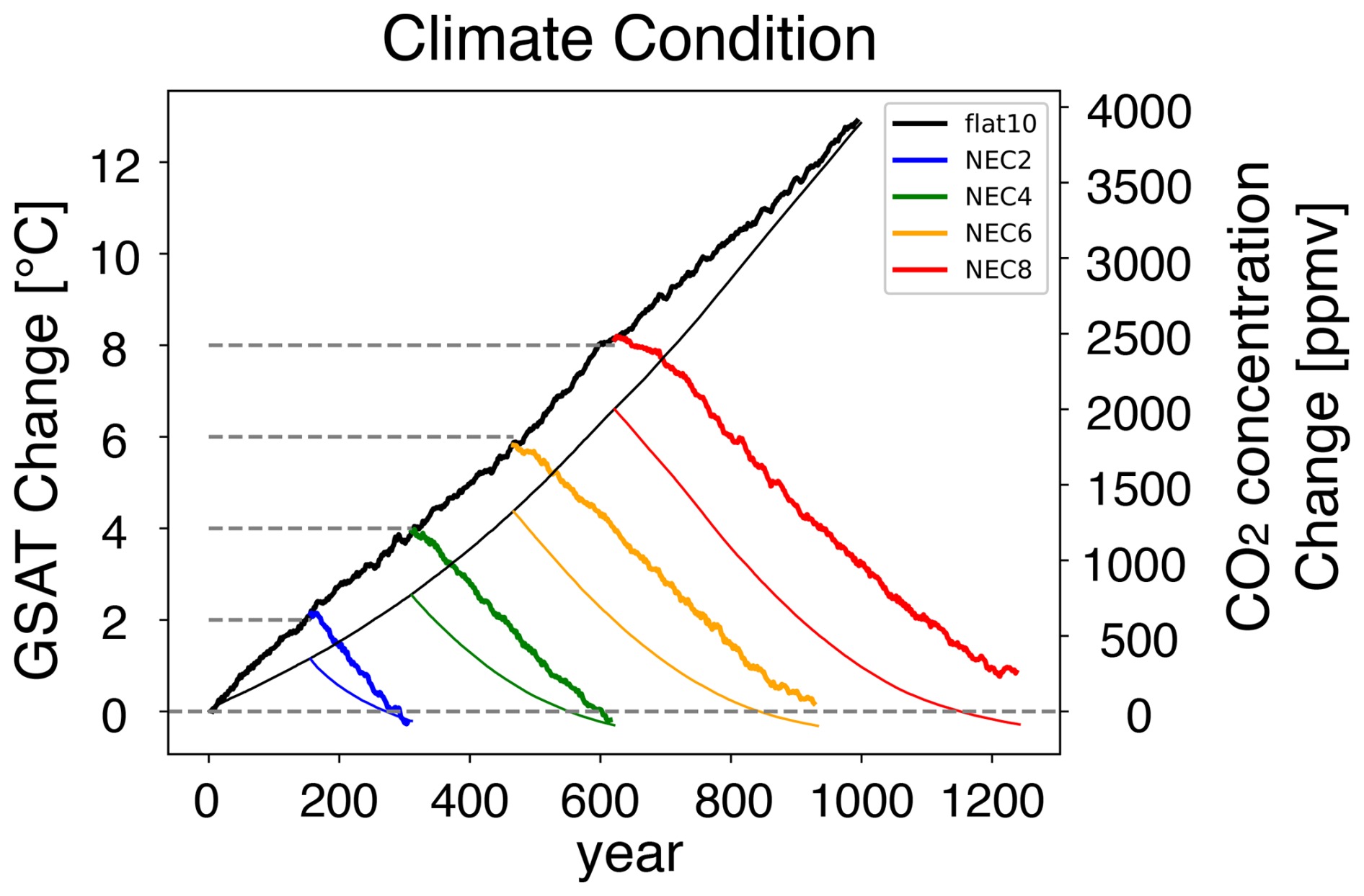
Figure 1 Timeseries of GSAT (thick) and CO₂concentration (thin) in idealized overshoot scenarios. Curves in black show the result of flat10 and colored curves show the results of NEC experiments (NEC2 in blue, NEC4 in green, NEC6 in orange, and NEC8 in red). The dashed lines denote the global warming levels where each NEC experiment is branched off from flat10. All the values are deviations from long-term means in the piControl run.

3.2 Permafrost area response to increase and decrease of CO₂ emissions

3.2.1 Hysteresis

Figure 2 shows the change in the NH permafrost area in response to global warming in the flat10 experiment. In its initial state, permafrost spreads across the entire high-latitude region covering the area of 2.5 × 10⁷ km², similar to the observed permafrost region of 2.1 × 10⁷ km² (Fig. 2a). We compared the permafrost extent diagnosed from MIROC-ES2L with observational data (Fig. S2). Although the overall distribution is well reproduced, particularly over northern Eurasia, the agreement is incomplete near the permafrost boundaries. In particular, there are substantial discrepancies in the mid- to high-latitude regions of North America compared with the observations. This discrepancy is attributable to a warm bias in surface air temperature over North America in MIROC-ES2L (Hajima et al., 2020).

When the GSAT increases from piControl by 2 °C, permafrost thaws near the edges but the area shows no significant change (Fig. 2b). However, most of the permafrost area over the North American continent is lost at a larger GSAT increase of 6 °C (Fig. 2c). The permafrost still remains over Siberia, but it also disappears when GSAT increases further. MATSIRO tends to project a low sensitivity to GSAT change compared to other land models because of little snow insulation (Burke et al., 2020).

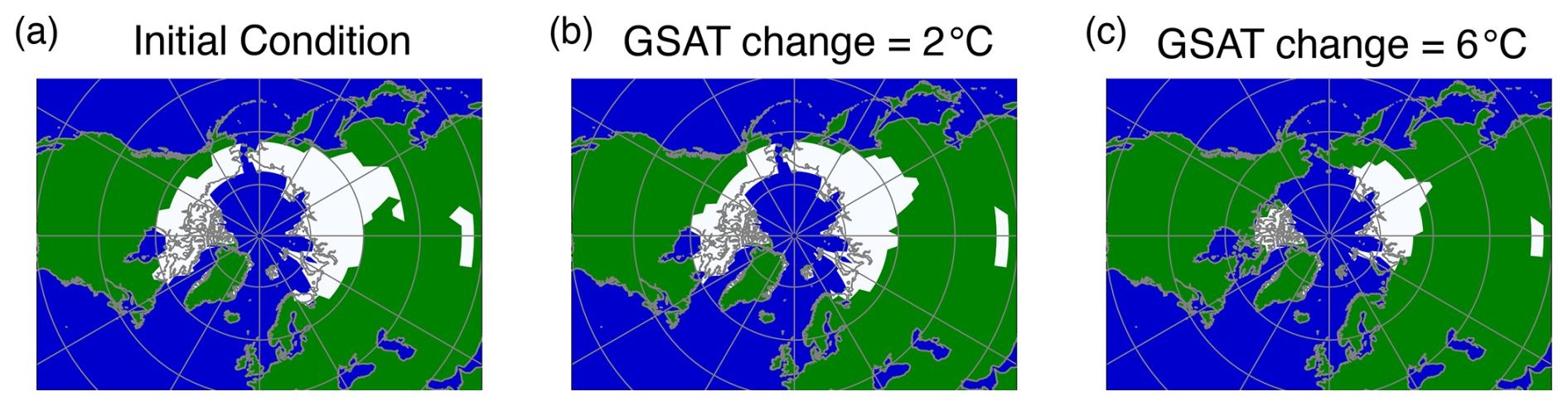
Figure 2 Permafrost areas (white) at different stages in the flat10 experiment: (a) initial state, (b) warmed state when the GSAT increases by 2 °C, and (c) warmed state when the GSAT increases by is 6 °C.

We examined the temporal evolution of the NH permafrost area (Fig. 3a). In the flat10 experiment, the permafrost area slowly declines at a rate of 0.05–0.25 × 10⁷ km² per century for approximately the first 250 years, followed by a rapid decrease of 0.44–0.60 × 10⁷ km² per century afterwards until about 750 years when permafrost thaws completely. In all experiments, permafrost continues to thaw for 100–200 years after branching off from flat10 despite GSAT has already started to decrease (Fig. 1). The delayed recovery of the permafrost area is rapid at the rate of 0.47–0.75 × 10⁷ km² per century, which is similar to the rapid permafrost loss in the flat10 experiment.

As the final states of NEC experiments show a similar area to the initial state of flat10 except NEC8 (Fig. 3a), the response of permafrost area to the increase/decrease of CO₂ emissions is regarded as largely reversible. Nevertheless, due to change in the thawing rate during the warming phase and a delay of recovery during the cooling phase, the trajectory of the permafrost area against the GSAT change shows a clear hysteresis (Fig. 3b). Exception is NEC2, which is branched off before the permafrost thawing changes its rate and therefore does not show a large hysteresis, and yet NEC2 shows a small but similar response to other NEC experiments in terms of the delay in the recovery during the cooling phase (Fig. 3a). Compared with Burke et al. (2020), the response of permafrost area to GSAT change obtained in this study is similar to that of MIROC6, whereas the result from MIROC-ES2L is close to an outlier. However, the sensitivity of permafrost area to GSAT change in MIROC-ES2L increases only after GSAT change reaches approximately 4 °C. This behavior can be attributed to the fact that the lowest soil layer in MATSIRO has a thickness of 10m, making it difficult for this layer to completely thaw under warming of less than 4 °C. Furthermore, when permafrost is defined as regions where at least one soil layer within a depth of 3 m satisfies the permafrost criteria, almost no hysteresis is observed.

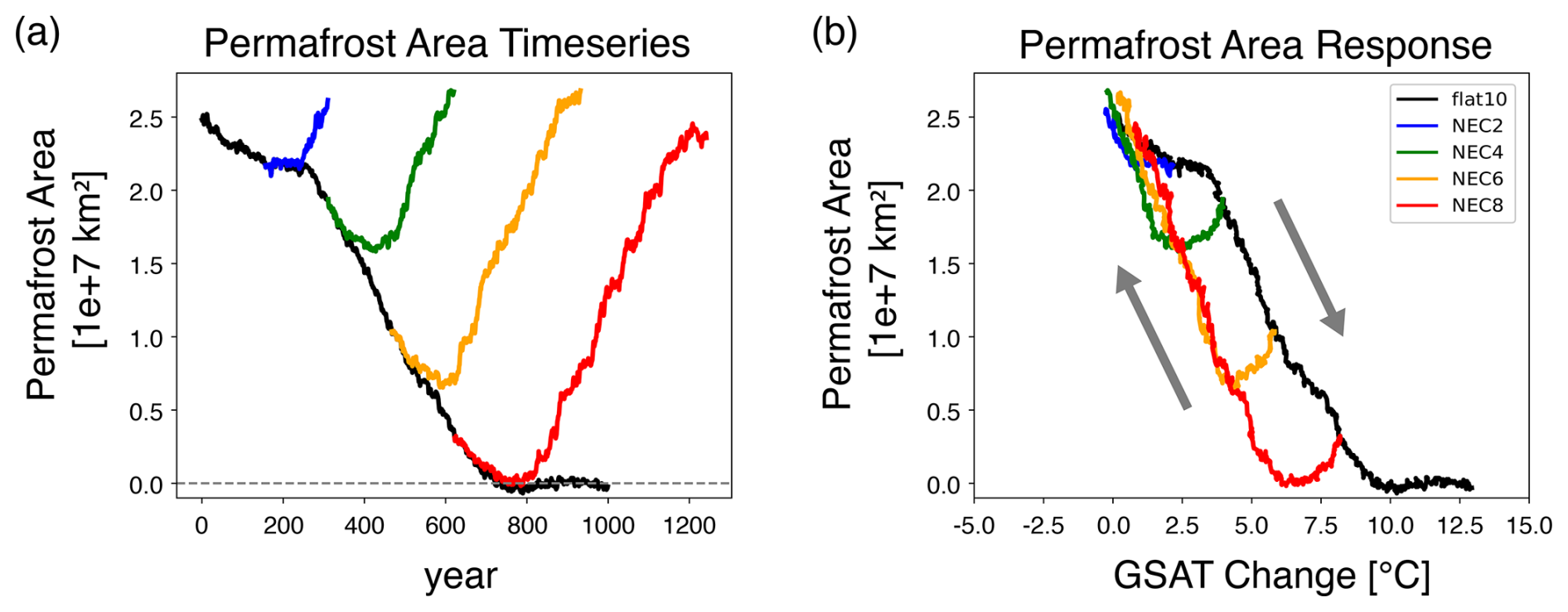
Figure 3 Response of permafrost area to global warming and cooling. (a) Timeseries of the NH permafrost area and (b) the trajectory as a function of GSAT change (grey arrows supplementarily show the direction of time evolution). Color convention follows Fig. 1.

3.2.2 The irreversibility in the bottom soil layer

In the following sections, we show the results of the NEC6 experiment as a representative case for understanding the permafrost hysteresis. In Fig. 4, we present again the GSAT and permafrost changes in flat10 and NEC6 experiments for a detailed comparison. Although the GSAT increase starts to reverse immediately after the emission change from positive to negative in around year 467 (dashed line in Fig. 4a), the permafrost thaw continues for the initial 150 years during the NEC6 experiment (Fig. 4b). The surface temperature in regions poleward of 60° N shows a similar response to GSAT but with a greater magnitude, indicating the Arctic amplification (Fig. S3), which does not explain the delay in the permafrost response.

The permafrost response at different soil layers shows that the delay of the permafrost recovery is roughly proportional to depth and the delay in the lowest soil layer (4–14 m) determines the characteristics of the total permafrost area (Fig. 4c). Moreover, a rapid decrease in permafrost area begins around years 250–300, coinciding with the start of thawing in the bottom layer (Fig. 4b, c). The recovery of permafrost area occurs when the upper layers (1–4 m) begin to re-freeze whereas the bottom layer remains thawed. Thus, the difference in the soil response at different depths to surface warming and cooling is the key to understanding the hysteresis response of the permafrost area. Note that the hysteresis in the permafrost area is not caused by the too-thick single bottom layer as we have confirmed it also happens in a one-dimensional soil model that has 100 soil layers (not shown).

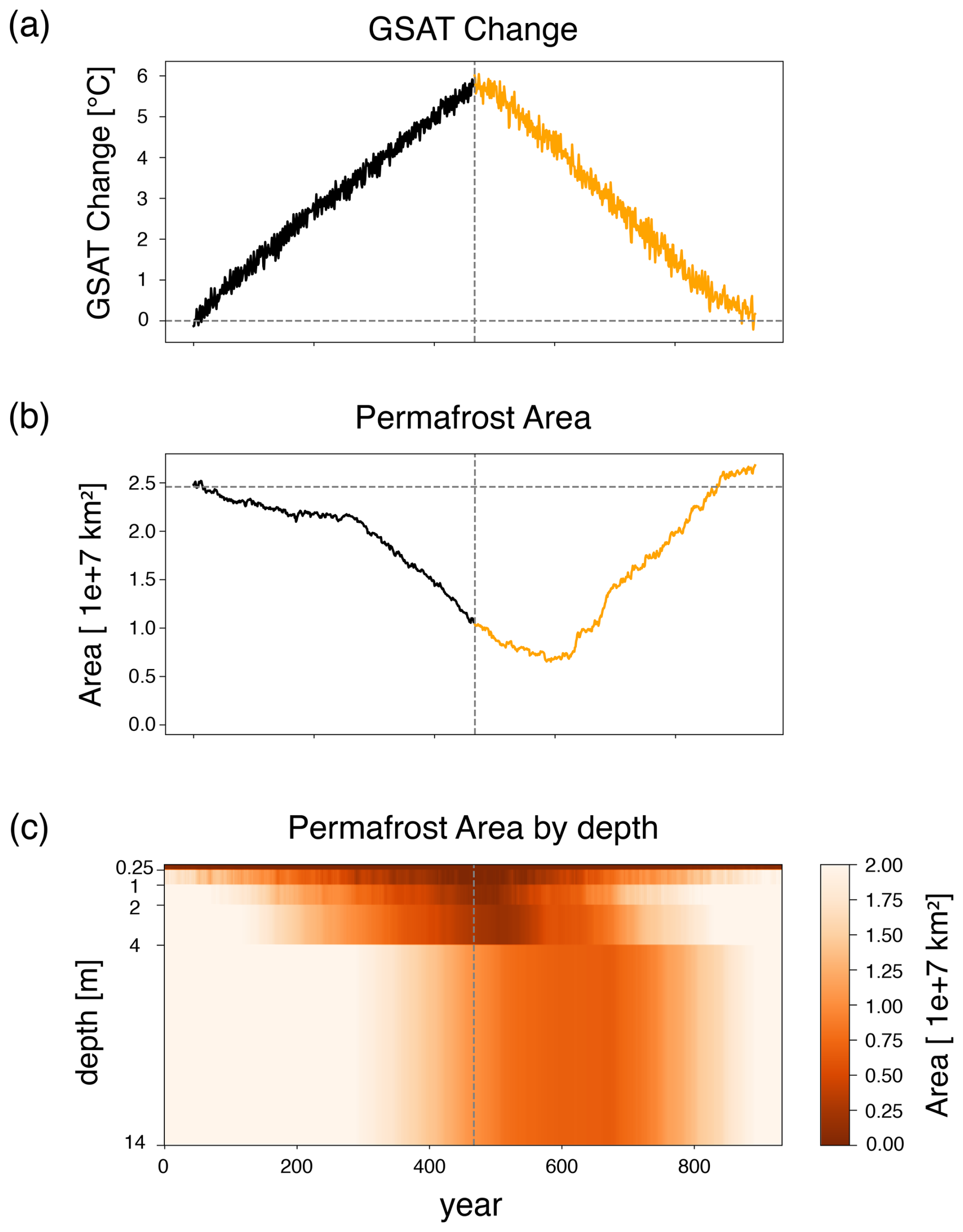
Figure 4 Time evolution of GSAT Change, NH permafrost area, and permafrost area by depth in flat10 and NEC6 experiments. (a) Timeseries of the GSAT change replicated from Fig. 1, (b) timeseries of the permafrost area replicated from Fig. 3, and (c) time-depth cross section of the area that meets the definition of permafrost layers. The vertical dashed line indicates the year when the flat10 run is switched to NEC6.

We also investigate the soil property such as reversibility of the ratio of frozen to liquid water changes in each soil layer in the flat10 and NEC6 experiments. Permafrost layers can be separated into a frozen layer with the annual maximum soil temperature below 0 °C and a mixed-phase layer with the annual maximum soil temperature remains at 0 °C. The former layer is called frozen or “ice” and the latter half-frozen or “sherbet”. We define sherbet layers as where the annual maximum soil temperature is just 0 °C. Thus, liquid and frozen water coexist in the sherbet layer and the rate of frozen water in sherbet layers is under 100 %. GHGs are not emitted from the ice layer, while emit from the sherbet layer. Therefore, the distinction between these two states is important when assessing GHG emissions due to permafrost thaw.

Delayed permafrost recovery during the global cooling phase, predominantly occurring in the deep soil layer (Fig. 4c), may be linked to the soil property change. Therefore, we compare distribution of ice and sherbet in the lowest soil layer (4–14 m) between the initial state of flat10 and the final state of NEC6 (Fig. 5). In the initial state of the flat10 experiment, most of the permafrost areas are ice and sherbet appears only in the periphery (Fig. 5a). In the final state of NEC6, in contrast, ice area shrinks and sherbet area extends in low latitudes (Fig. 5b).

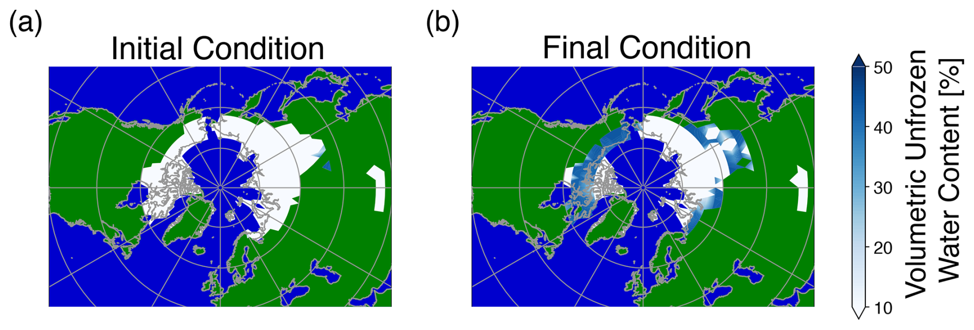
Figure 5 Soil property in the bottom layer (4–14 m) in (a) the piControl experiment and (b) the last year of the NEC6 experiment. Note that GSAT is nearly the same between the two states. Regions in white indicate ice areas, while in blue indicate sherbet areas where the water phase change is undergoing (darker blue denotes a larger amount of unfrozen water).

The irreversible change in the ice and sherbet areas can be clearly seen in their trajectory against the GSAT change (Fig. 6). In the bottom layer, the ice area decreases with warming and recovers with cooling but at a slower rate, leading to a smaller ice area in the final state of the NEC6 experiment (Fig. 6a). The area of sherbet regions increases until the GSAT reaches around 3 °C, when the permafrost area begins to decrease rapidly (Fig. 4a, b). This transition occurs because the sherbet areas initially expand in relatively low-latitude regions during the early phase of warming, but they thaw at a threshold of ground temperature increase that is proportional to the GSAT increase. In NEC6, the sherbet area continues to decrease until GSAT down to around 3 °C and after which it begins to increase (Fig. 6b). In the final state of NEC6, the sherbet area is larger than the initial state. Note that the sum of ice and sherbet areas in the bottom layer is roughly the same in the initial and final states (Fig. 4c). These irreversible changes are not clear in the upper soil layer (Fig. 6c, d). In addition, soil moisture exhibits increasingly irreversible behavior with depth, with a larger decrease observed in relatively low-latitude regions.

Soil moisture shows a decrease in all ground layers in the flat10 experiment and an increase in the NEC experiments (Figs. S4, S5). The soil moisture response exhibits irreversibility as in the permafrost property of the ratio of frozen to liquid water, particularly in the deeper layers. While soil moisture in the layer shallower than 2 m can be considered reversible and does not demonstrate hysteresis, the recovery during the NEC experiment remains insufficient in the layers below that depth.

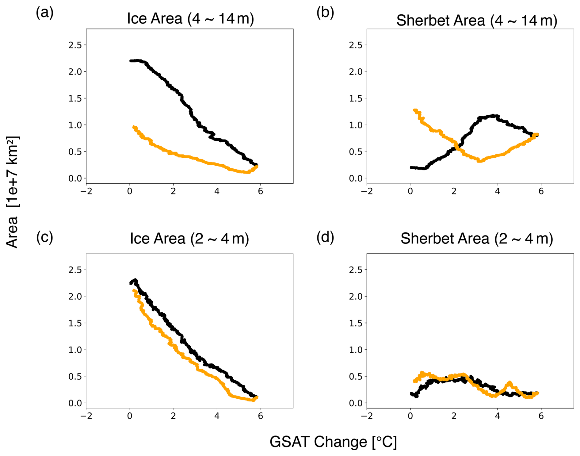
Figure 6 Response of soil property to warming and cooling in the bottom (4–14 m) and upper (2–4 m) layers. Trajectory of (a) ice and (b) sherbet areas in the bottom layer as a function of the GSAT change in flat10 (black) and NEC6 (yellow). (c)–(d) As in (a)–(b) but in the upper layer.

3.3 Factors contributing to hysteresis and irreversibility of permafrost response

During the global warming, radiative forcing heats the ground and the excess heat is then transferred downward in the soil, causing thawing from upper to lower layers, as schematically depicted in Fig. 7a (left two panels). During the thawing period, excess heat is first used to change the phase from ice to sherbet, without much decrease in the total permafrost area. Once the GSAT change reaches a critical threshold (around 3 °C in flat10), the sherbet begins to melt, leading to the rapid decrease of the permafrost area (middle panel).

During the subsequent cooling phase, heat is transferred from the near-surface soil to the atmosphere, leading to the decrease in the near-surface soil temperature and the freezing from upper layers. In the meantime, thawing continues in the lower soil layers. Near-surface layer is affected by seasonal temperature variations, so the permafrost recovery occurs in the middle of soil layers and continues until the bottom layer freezes (right two panels). Therefore, the vertical structure of frozen soil is different between the warming and cooling phases at the same global warming level. After the start of the permafrost area increase during the cooling phase, the frozen area in the upper soil layers (1–4 m) expand but not in the bottom soil layer (Figs. 4c, 6). At this point, the permafrost area is approximately equal to the area where the upper layers (1–4 m) are frozen (Figs. 4b, 6c, d). This is because a larger area of regions satisfies the permafrost definition in the upper layers than in the bottom layer. Thus, the phase of gradual thawing in the warming experiment and the phase of continued thawing in the cooling experiment together form the transition connecting the two periods which are different in the representative soil layers. This is the way that the permafrost hysteresis happens.

In addition, because freezing starts from the upper soil layers during the cooling phase, there are regions where freezing in the lower soil layers has not yet fully progressed, consisting of sherbet. As a result, the area of sherbet regions increases and the area of ice regions decreases in the bottom soil layer at the end of NEC experiments, compared to the initial state (Figs. 5, 7a).

The above thawing and refreezing mechanisms are inferred from the results of flat10 and NEC6 experiments (Figs. 3, 4, 6). To verify them, we conducted a series of sensitivity experiments. We consider two possible factors that lead to the delay of the bottom soil layer response to GSAT change. The first factor is the effect of soil heat conductivity and the second factor is the effect of specific heat of water, i.e., heat required for the phase change between ice, sherbet and water, which may explain the rate change of the permafrost thawing as well as the delay in the permafrost recovery. Both factors can cause the delay in heat transfer to the soil layers but through different mechanisms. In the next section, we verify the above hypothesis for the mechanisms of hysteresis by performing sensitivity experiments designed to assess the effects of soil heat conductivity and specific heat on hysteresis and irreversibility of permafrost response.

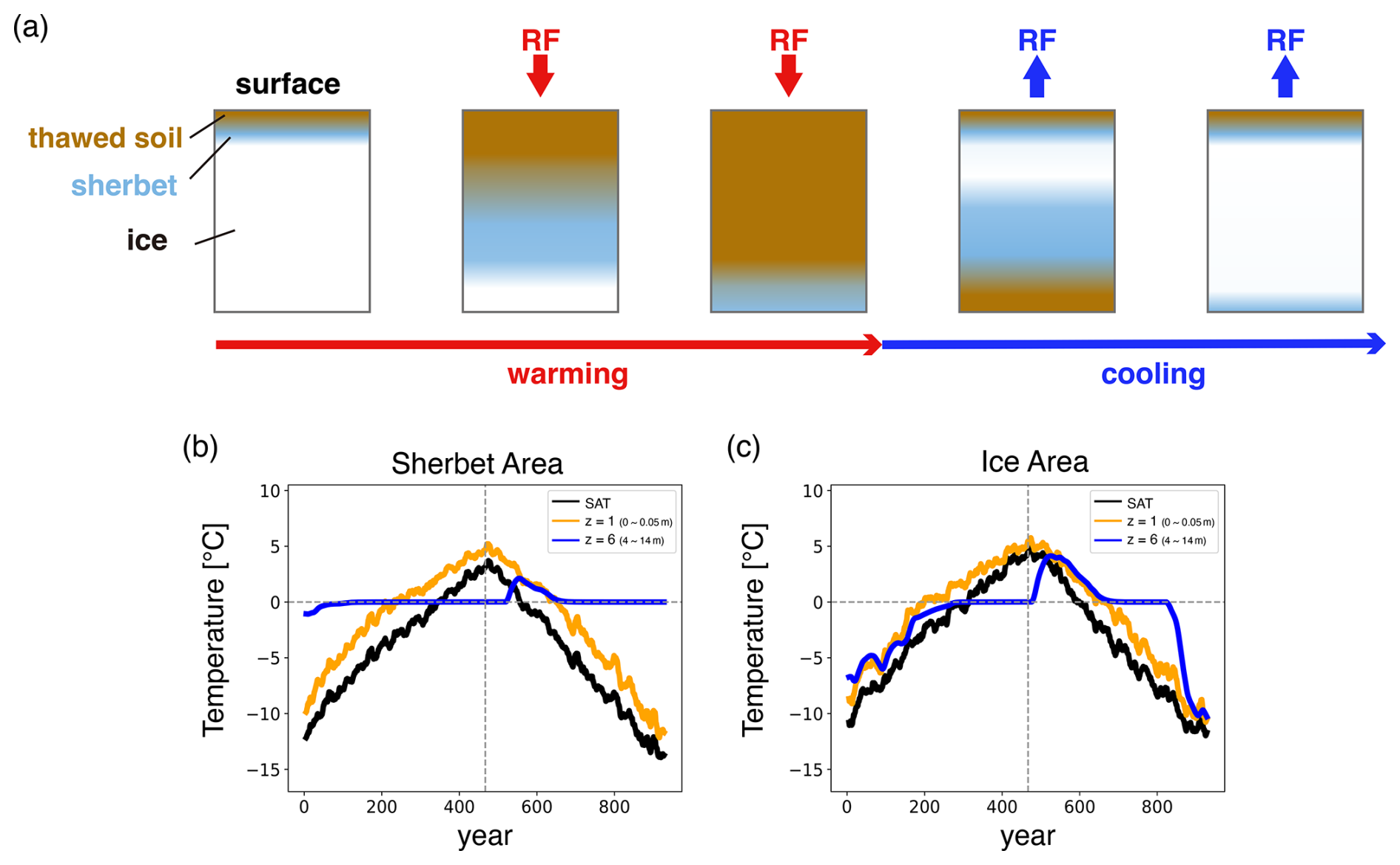
Figure 7 Schematic explaining hysteresis and irreversibility of the physical permafrost during thawing and re-freezing. (a) Five rectangular panels show the vertical cross sections of the soil, representing the initial state of warming (leftmost), followed by the warming states during and at the end of the flat10 experiment, and the two cooling states during and at the end of the NEC experiment. Radiative forcing and the SAT changes are shown by arrows. (b, c) Timeseries of annual-mean temperature in regions where the bottom layer (4–14 m) is sherbet (b: 68° N, 87° W) and ice (c: 71° N, 171° E) at the end of the NEC6 experiment. The black curves represent the SAT, and the brown and blue curves represent the ground temperature at the surface layer (0–0.05 m) and the bottom layer, respectively. The vertical dashed line indicates the year when the flat10 run is switched to NEC6.

3.4 Sensitivity experiments

Two types of sensitivity experiments were conducted based on flat10 and NEC6 by varying the soil heat conductivity or the specific heat of water. The soil heat conductivity in MATSIRO is defined as

$$\begin{array}{}\text{(8)}& k_{g\left(z\right)}=k_{g\mathrm{0}\left(z\right)}\left[\mathrm{1}+f_{kg}\tanh \left({\displaystyle \frac{w_{\left(z\right)}}{w_{kg}}}\right)\right]\end{array}$$

where k_g(z) and k_g0(z) represent the heat conductivity and its coefficient at depth z [m], respectively. f_kg and w_kg are constant, and w_(z) represents the soil moisture at depth z [m]. The units for k_g and k_g0 are [W/(m K)], and the unit for w_kg is [m³ m⁻³]. To modify the effect of heat conductivity, a prescribed parameter k_g0(z) is varied by multiplying factors of $\mathrm{1}/\mathrm{2}$, 2, and 10 in the sensitivity experiments and then we repeated flat10 and subsequent NEC6 experiments.

In MATSIRO, the amounts of melted or frozen soil moisture are calculated by Eq. (9).

$$\begin{array}{}\text{(9)}& \mathrm{\Delta }{\mathit{\theta }}_i=C_g\left(T_{\mathrm{mlt}}-T_g\right)/{\mathit{\rho }}_{\mathrm{w}}{l}_{\mathrm{mlt}}\end{array}$$

Δθ_i represents change in the amount of frozen water present in the soil [m³], C_g is heat capacity of soil [J K⁻¹], T_mlt is melting temperature of 273.15 [K], T_g is soil temperature [K], ρ_w is the density of water [kg m⁻³], and l_mlt is the specific heat for the phase change between frozen water and liquid water [J kg⁻¹]. To modify the effect of latent heat associated with the water phase change in the soil, a prescribed parameter l_mlt is perturbed by multiplying factors of 2, $\mathrm{1}/\mathrm{2}$, and $\mathrm{1}/\mathrm{10}$ in the sensitivity experiments and then we repeated flat10 and subsequent NEC6 experiments.

The results of perturbing soil heat conductivity are summarized in Fig. 8a–c for the permafrost area, ice and sherbet areas against GSAT changes. The permafrost hysteresis is smaller with doubling of heat conductivity and vice versa with halved value (red and blue curved in Fig. 7a). In an extreme case with the heat conductivity 10 times as large as the standard parameter, hysteresis roughly diminishes (yellow curve). Unlike the high sensitivity of the permafrost area response, the permafrost properties, i.e., redistribution between ice and sherbet in the bottom soil layer are insensitive to perturbed heat conductivity (Fig. 8b, c). Although a large heat conductivity acts to slightly weaken irreversibility, soil heat conductivity is not likely the major cause of irreversibility in the permafrost properties.

The results of changing specific heat of phase change are summarized in Fig. 8d–f for the permafrost area, ice and sherbet areas against GSAT changes. The permafrost hysteresis is larger with halved value of specific heat and vice versa with doubling value (blue and red curved in Fig. 8d). In an extreme case with the specific heat $\mathrm{1}/\mathrm{10}$ times as large as the standard parameter, hysteresis almost completely diminishes (purple curve) and becomes smaller than that in extreme case with the heat conductivity 10 times. Specific heat for water phase change is found to affect the irreversible character of ice and sherbet areas, too (Fig. 8e, f). In particular, an extreme case of reducing latent heat parameter to $\mathrm{1}/\mathrm{10}$ shows that both ice and sherbet areas are almost reversible (purple curves). This can be interpreted as the reduced specific heat making frozen (or half-frozen) soil melt more easily during global warming, prohibiting sherbet area to increase. Likewise, soil moisture can freeze more easily during global cooling, enabling the sherbet soil to freeze rapidly.

Based on the results of two types of sensitivity experiments, we conclude that the permafrost hysteresis and irreversibility are affected by both the heat conductivity effect and the specific heat effect, but the latter has a greater influence. This interpretation is consistent with previous studies (Cox et al., 1999; Eliseev et al., 2014) showing that the hysteresis of permafrost is influenced by an increase in the apparent heat inertia of soil caused by phase transitions. It is also worth noting that no differences were found in atmospheric temperature or CO₂ concentration between the standard experiments and these sensitivity experiments. The key to determine whether the bottom soil layer returns to ice or remains in sherbet at the end of NEC experiments is the time required for the phase change. Even when surface temperatures are similar, a longer phase change time makes it more difficult for all soil moisture to refreeze during NEC experiments (Fig. 7b, c). The time required for phase change is proportional to the amount of soil moisture. Naturally, high-latitude regions tend to freeze faster due to low temperature unlike middle latitudes where sherbet remains longer time.

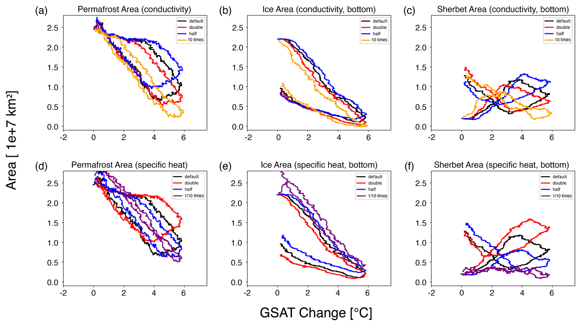
Figure 8 Response of the NH permafrost area (cf. Fig. 3b) and soil property in the bottom layer (4–14 m) (cf. Fig. 6) to warming and cooling in the modified flat10 and NEC6 experiments. The upper panels show the results with perturbing soil heat conductivity, and the lower panels show the results with perturbing specific heat of water phase change; doubling (red), halved (blue), 10 times (orange in upper panels), $\mathrm{1}/\mathrm{10}$ times (purple in bottom panels) values of the parameters imposed on the standard cases (black). (a, d) Response of permafrost area, (b, e) response of ice area, and (c, f) response of sherbet area, respectively. The thick curves indicate the 11-year running mean of GSAT change.

3.5 Estimated amount of GHGs emission from permafrost thaw

The cumulative emissions of CO₂ and CH₄ released from thawed permafrost in the flat10 and NEC experiments are estimated by offline calculation using PDGEM (cf. Sect. 2.4). As GSAT increases, the cumulative emissions of CO₂ and CH₄ also increase but at a rate varying in time such that the emission is slow during the early and late stage of warming but rapid in between (Fig. 9). The carbon release from thawed permafrost during a GSAT change of 0–4 °C is approximately 14PgC per degree of global warming, which falls within the uncertainty range of 3–41 PgC estimated by Winkelmann et al. (2023). As expected from the permafrost hysteresis, GHGs emissions from thawed permafrost continue for some time after warming in flat10 turns to cooling in the NEC experiments. In NEC2, for example, the cumulative CO₂ emissions from permafrost reach approximately 10.9 PgC, accounting for 41.3 % of the total cumulative permafrost emissions from the beginning of flat10 to the end of NEC2. On the other hand, there is little GHGs emission during the NEC8 experiment that accounts for 0.6 % of the total cumulative emissions throughout the experiments because all the NH permafrost has almost thawed at this warming level. The impact of the permafrost hysteresis on carbon releases is not negligible but depends on the global warming level when the GHGs emission turns about from positive to negative. This finding indicates that permafrost hysteresis may have a significant impact on additional GHGs emissions, especially under a modest warming level of 2 °C. Furthermore, carbon emissions from thawed permafrost induce additional warming. The contribution to the GSAT increase is estimated as 0.19  °C at 2 °C warming, 0.60 °C at 4 °C warming, 0.82 °C at 6 °C warming, and 0.96 °C at 8 °C warming (Fig. S6), indicating that the permafrost feedback amplifies the warming by 10 %–15 %. In addition, offsetting carbon emissions from permafrost requires extending the duration of the negative emission period by approximately 12 %–17 % (data not shown).

Our calculation has limitations on top of the lack of feedback between climate and carbon release from the permafrost thaw. Namely, PDGEM assumes that once the frozen soil thaws, it continues to emit GHGs even after refreezing (cf. Sect. 2.4). This differs from the actual response of permafrost under climate cooling. Since GHGs emissions from a thawed soil are assumed to continue for 15 to 40 years, this assumption would act to overestimate the GHGs emissions from permafrost soils that refreeze before the emissions have finished. During flat10 and NEC experiments, the volume of regions that begin to refreeze before the GHGs emission finishes accounts for approximately 40 % in NEC2, 20 % in NEC4, 15 % in NEC6, and 10 % in NEC8 experiment of the total volume of areas that no longer meet the definition of permafrost by the end of experiments. This means that the model calculates GHG emissions from soils that have actually started to refreeze and would have suppressed emissions, in the same manner as from thawed soils, leading to an overestimation of total GHG emissions. Of the CO₂ emitted from soils after the start of the NEC experiments, up to approximately 4.34 PgC in NEC2, 1.38 PgC in NEC4, 1.06 PgC in NEC6, and 0.05 PgC in NEC8 can be overestimated. Similarly, of the CH₄ emitted from soils after the start of the NEC experiments, up to approximately 0.355 PgC in NEC2, 0.113 PgC in NEC4, 0.071 PgC in NEC6, and 0.003 PgC in NEC8 can be overestimated. Furthermore, SOC is in reality abundant in the upper soil layers, but the model assumes a uniform vertical distribution of soil carbon. This may also cause a potential overestimate of the effect of hysteresis on the GHGs emissions from permafrost. In contrast, GHG emissions from sherbet regions, which would occur in nature, are not assumed in PDGEM, causing an underestimation of the GHGs emissions. Given these potential errors that act to overestimate and underestimate the carbon emission, our results may still be subject to uncertainty.

High-emission scenarios resulting in a greater warming lead to a large permafrost thaw. In addition, the calculation of carbon emissions from thawed permafrost can be assumed that the relationship between the temperature change and carbon release from permafrost is unique across scenarios. Using this assumption, we compare the permafrost carbon emissions under the SSP scenarios with the results from the flat10 experiment, using temperature as a common metric. Under the SSP5-8.5 scenario, with a projected GSAT change of about 5.5 °C (IPCC, 2021), cumulative emissions from permafrost thaw are estimated to be 46.5 PgC (31–63 PgC) for CO₂ and 2050 Tg CH₄ (1250–2800 Tg CH₄) by the end of this century (Yokohata et al., 2020a). Regarding the results of our flat10 experiment when the GSAT change reached 5.5 °C, the cumulative CO₂ emissions from permafrost remained within the uncertainty range mentioned above. In contrast, CH₄ emissions from permafrost exceeded the projected uncertainty range. This discrepancy may be attributed to differences in the temperature response to scenarios among various models, as well as variations in the simulated distribution of wetlands and drylands. Given these findings, we can say that the uncertainty range for CH₄ emissions from permafrost at warming levels exceeding 6 °C could be even larger than the values reported in the SSP5-8.5 experiments by Yokohata et al. (2020a). Furthermore, CH₄ emissions are expected to follow a similar trend to CO₂. In addition, the inherently large volume of CH₄ emissions further amplifies the overall uncertainty, leading to an even wider range of projected values. Furthermore, while other Earth system feedbacks associated with permafrost exist, they are outside the scope of this study. Our analysis focuses on GHG emissions from permafrost thaw.

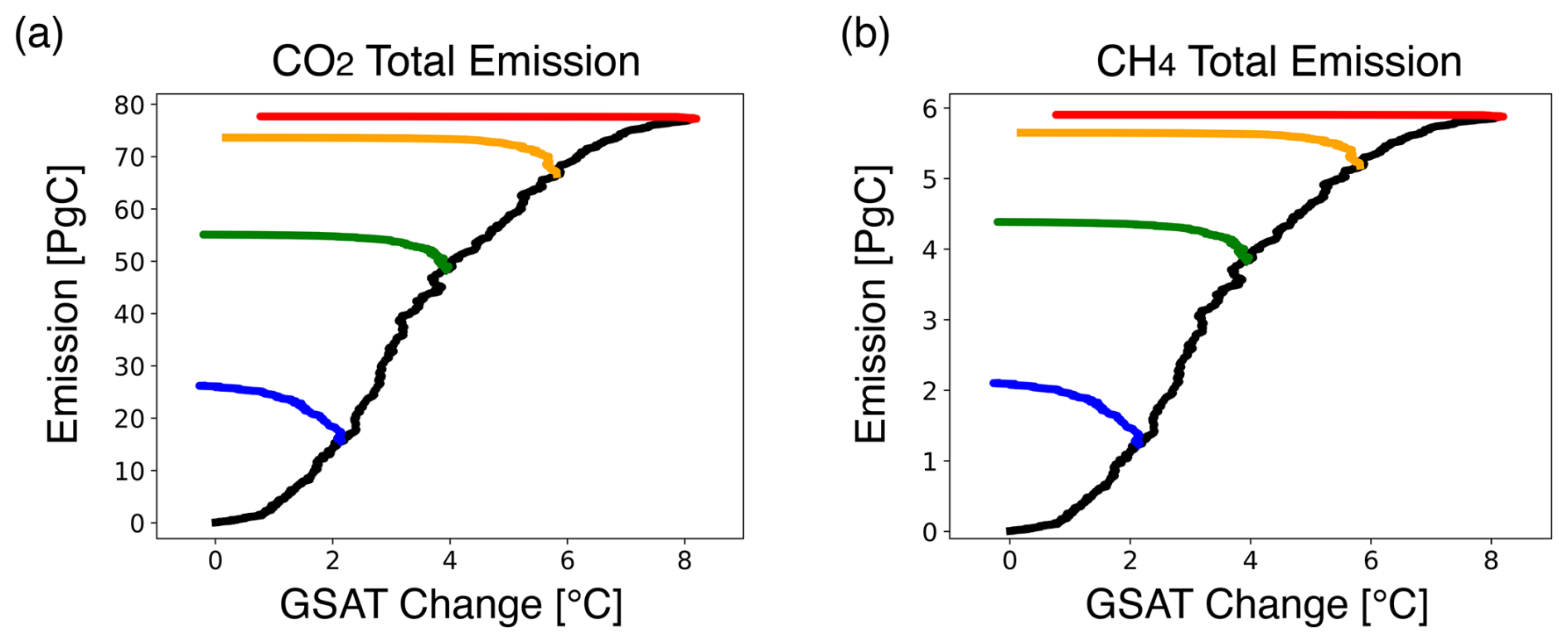
Figure 9 GHGs emission from permafrost thaw. NH cumulative emissions of (a) CO₂ and (b) CH₄ in response to GSAT change. Color convention follows in Fig. 1.

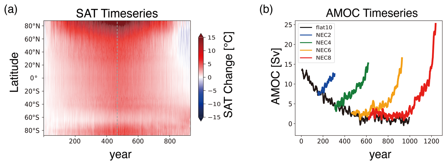
Figure 10 Hysteresis and irreversibility in the large-scale climate indicator. (a) Response of annual- and zonal-mean surface air temperature in flat10 and NEC6. The vertical dashed line indicates the year when flat10 is switched to NEC6. (b) Timeseries of the 11-year running mean AMOC index (maximum value of the meridional stream function at 34° N) in flat10 and the four NEC experiments. The color convention follows Fig. 1.

4 Discussion

We have shown that permafrost has hysteresis in its area and irreversibility in its properties (i.e., ice and sherbet) during the global warming and subsequent cooling regardless of the global warming level when the cooling starts. The results described in the previous section are consistent with other modeling studies. Park et al. (2025) demonstrated that permafrost thawing and the subsequent release of GHGs continue even after anthropogenic CO₂ emissions transition to negative levels, which aligns with the findings of this study. Furthermore, Boucher et al. (2012) pointed out the existence of hysteresis in the response of the permafrost area to climate change, a phenomenon that is also consistent with our results. These permafrost responses can be explained by local physical processes of the soil layers. However, the permafrost response may also be influenced by non-local processes in the Earth system. We discuss in this section such possibilities by looking at large-scale climate indicators.

In the NH high latitudes, the surface air temperature is lower at the final state of NEC6 than at the initial state (Fig. 10a). This cooling can be attributable to the delay of the Atlantic Meridional Overturning Circulation (AMOC) response. It is known that AMOC exhibits hysteresis and become stronger than its initial state during the recovery phase (Wu et al., 2011; Jackson et al., 2014; An et al., 2021). Consistent with them, the NEC simulations show that the AMOC recovery delays more when the NEC experiment is started from a higher global warming level, whereas its final state is stronger than the initial state (Fig. 10b). Since the AMOC transports a large amount of heat from lower to higher latitudes, the surface cooling shown in Fig. 10a is likely explained by the delayed recovery of the AMOC. The AMOC final state is stronger than the initial state, but it does not affect the temperature response in the NH during the NEC experiments because the temperature response lags behind the AMOC. The colder NH surface condition would have acted to help refreezing of the soil moisture. Therefore, the influence of AMOC hysteresis does not explain the hysteresis and irreversibility in permafrost and may have even counteracted them.

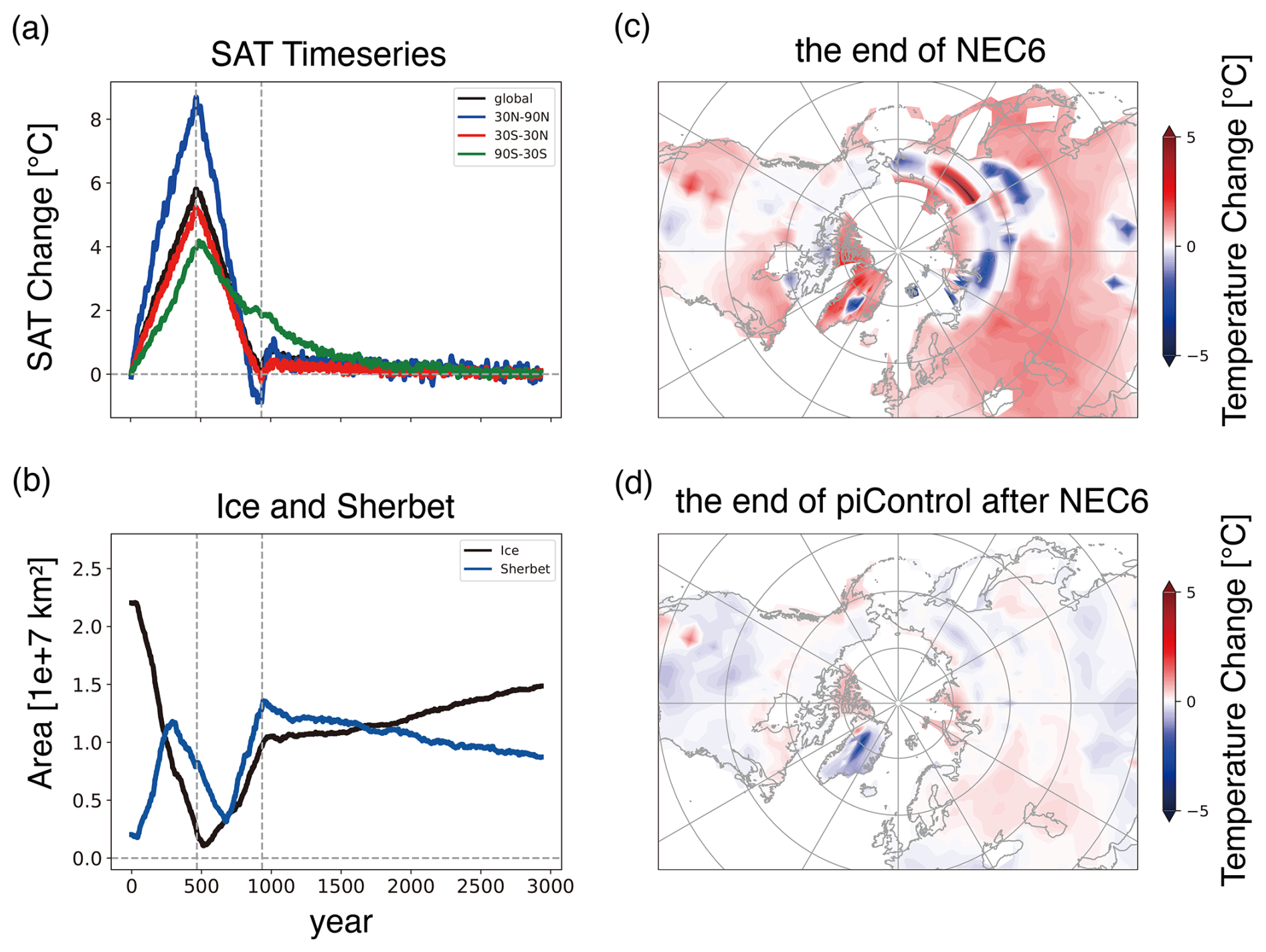
Figure 11 (a, b) Timeseries in flat10, NEC6, and the 2000-year piControl run after NEC6 experiment. The vertical dashed lines indicate the year when the flat10 run is switched to NEC6 and to piControl. (a) Response of the annual-mean GSAT (black) and SAT averaged over 30–90° N (blue), 30° S–30° N (red), and 30–90° S (green). (b) Timeseries of ice (black) and sherbet (blue) areas. (c–d) Difference of the 10 year-mean soil temperature in the bottom layer (4–14 m) from piControl in (c) the end of NEC6 and (d) the 2000-year piControl experiment conducted after NEC6.

Although some measures such as GSAT, global-mean CO₂ concentration, and the NH permafrost area, are roughly reversible to the CO₂ emissions, climate system in detail has not turned back to the initial state as evident from the permafrost properties, surface temperature pattern, and AMOC. To further investigate the equilibration of the permafrost, a 2000-year piControl experiment following the NEC6 experiment was conducted. During this extended piControl experiment, the heat is transported from the Southern Hemisphere to the NH, reducing the temperature contrast between them (Fig. 11a). Although GSAT increases immediately after NEC6 was switched to piControl, it gradually decreases thereafter and eventually returns to the initial state. The temperature difference between the hemispheres nearly vanishes after 2000 years and then equilibrated. Also, the permafrost ice and sherbet areas in the bottom soil layer gradually increases and decreases, respectively, during the extended piControl experiment and approach the initial states (Fig. 11b). However, the permafrost property of the ratio of frozen to liquid water in lowest soil layer may not fully recover to the initial state when the climate reaches equilibrium.

As inferred from Fig. S1, TCRE shows neither irreversibility nor hysteresis in our experiments, but this may be model-dependent (Sanderson et al., 2024). Koven et al. (2022) evaluated the irreversibility of TCRE using six ESMs under the SSP5-3.4OS scenario. While TCRE was generally similar across models, differences in sign and magnitude of ZEC were identified among models and they were a major source of uncertainty in future temperature decline under stabilization scenarios. Therefore, taking inter-model differences in TCRE and ZEC into account would be important for improving our understanding of permafrost–climate interactions.

Despite the NH surface is colder at the final state of NEC6 compared to the initial state of flat10 (Fig. 11a), the sherbet areas still widely exist in the bottom soil layer (Fig. 5b). This is because the surface cooling pattern is not uniform (Fig. 11c). In the NH high latitudes where the bottom soil layer is colder at the end of NEC6 than at the initial state, permafrost has been recovered (Fig. 5b). In the area outside the cold region, where soil temperatures are either slightly higher than or nearly equal to the initial state, the sherbet area remains. After 2000 years of the extended piControl, the spatial non-uniformity in temperature in the bottom soil layer becomes much smaller and temperatures in most regions return to values in the initial state (Fig. 11d).

Furthermore, a negative emission rate of −10 PgC yr⁻¹, as prescribed in the NEC experiment, may actually be unattainable. Yet the mechanisms of permafrost physical response clarified using such idealized scenarios would be qualitatively applicable for the response under more realistic emission pathways.

5 Conclusions

To clarify the permafrost physical response – irreversibility, hysteresis, and their mechanisms – to increase and decrease in the CO₂ emissions, we conducted idealized warming (flat10) and cooling (NEC) experiments using MIROC-ES2L, one of the Earth System Models participating in CMIP6, and then obtained the following results. First, the permafrost area is reversible between the initial state of the warming experiment and the final state of the subsequent cooling experiment, but exhibits hysteresis between the warming and cooling phases. This hysteresis arises primarily during the warming when the thawing speed becomes fast at a certain threshold and during the early stage of the cooling when the permafrost recovery is delayed. Second, the property of the permafrost such as the ratio of frozen to liquid water in the lower soil layer is irreversible. The area of frozen (ice) ground is reduced while the area of half-frozen (sherbet) ground expands when the climate has turned back to the reference state. These hysteresis and irreversibility are coupled and caused by the delay of heat conduction to lower soil layers. The hysteresis in the permafrost area becomes smaller with a larger heat conductivity and/or a smaller specific heat associated with the phase change of soil water. Both heat conductivity and specific heat in phase change contribute to hysteresis, but the latter plays a more substantial role.

Once thawed, the permafrost area would continue to release GHGs even under zero or negative emission because the frozen soil layer does not recover immediately. The extent and duration of additional thawing in the NEC experiments vary depending on the global warming level at which the CO₂ emissions are turn to negative. When the NEC experiments is started at a certain warming level of 3 °C or higher, the bottom soil layer continues to thaw for a longer time. As a result, the hysteresis becomes pronounced and the permafrost recovery takes a longer time. This suggests an importance of mitigating global warming with 2 °C is critical to avoid the permafrost hysteresis to occur. However, additional GHG emission from the thawed permafrost contributes more to the total cumulative permafrost emissions when the warming is mitigated at a smaller level. Cumulative permafrost CO₂ emissions up to the 2 °C threshold are approximately 16 PgC, followed by approximately 11 PgC of committed emissions during the NEC2 phase. Thus, the GHGs released from permafrost during the NEC experiment are significant, and it can be inferred that this will have a major impact when estimating the remaining carbon budget.

Clarifying the influence of permafrost thawing on climate warming is a critical issue for society, too. In this study, we estimate the impact of GHGs emissions from thawed permafrost by using an offline model. Ideally, this process should be interactively implemented in the ESM to fully represent the carbon-climate feedback. Furthermore, developing land surface models with improved representation of the SOC spatial distribution and GHGs emission processes are essential for reducing uncertainties in the GHGs emissions from thawed permafrost. In addition to GHGs emission associated with gradual thaw, understanding other effects of abrupt thaw such as wildfires and thermokarst formation triggered by ice wedge melting as well as the heat release from microbial activity are crucial for a comprehensive understanding of the permafrost as a tipping element.