
the Creative Commons Attribution 4.0 License.
the Creative Commons Attribution 4.0 License.
 | 13 Aug 2026
Catalogue of strong nonlinear surprises in ocean, sea-ice, and atmospheric variables in CMIP6
Joran R. Angevaare
Sybren S. Drijfhout

The Coupled Model Intercomparison Project Phase 6 (CMIP6) archive was analysed for the occurrence of Strong Nonlinear Surprises (SNS) in future climate-change projections. To this end, we built an automated detection algorithm to identify SNS in a reproducible manner. Two different types of SNS were addressed: abrupt changes measured over decadal timescales and state transitions developing over multiple decades, too large to be explained by the forcing without invoking strong internal feedbacks in the climate system. We also discuss when one SNS case features a cascade from one variable to another (where sea-ice, deep convection, and temperature and salinity changes interact) and when two SNS interact to form a cascade, which occurs for the subpolar mixed-layer collapse triggering an Atlantic Meridional Overturning Circulation (AMOC) shutdown. Data from 54 models were analysed for five shared socio-economic pathways for ocean, sea ice, and atmospheric variables that are involved in the coupling to ocean and sea ice. The algorithm isolates regions of at least 106 km2 and utilizes stringent criteria to select SNS. In total 73 SNS were found, divided in 11 categories of which 4 apply to abrupt change and 7 to state transitions. Of the identified SNS 45 % relate to sea-ice cover, 19 % to ocean currents, 29 % to mixed-layer depth, and 7 % to atmospheric systems like the Intertropical Convergence Zone. For each category, probability density functions for time-windows of maximal change indicate SNS occurring earlier and at lower global temperature rise than assessed in previous reviews, in particular the ones associated with winter Arctic Sea ice disappearance, northern North Atlantic winter mixed-layer collapse and subsequent transition of the AMOC to a weak state in which the cell associated with North Atlantic Deep Water formation has vanished.
- Article
(13427 KB) - Full-text XML
- BibTeX
- EndNote


Based on a literature review and an expert elicitation workshop, the concept of Climate Tipping Points was introduced and formalized by Lenton et al. (2008). They recognized that elements of the Earth System can qualitatively change their mode of operation when passing a critical threshold, the latter being popularized as a tipping point. Recent updates of this overview were given in Armstrong McKay et al. (2022), relating the possible tipping to the 1.5 °C global warming threshold, and in Loriani et al. (2025), based on a new assessment by a team of experts. After 2008, a large body of literature appeared discussing specific climate tipping points and subsequent socio-economic tipping points, associating the climate tipping point concept with anthropogenic climate change, its impacts and risks, and policy (Kopp et al., 2025).
In the latest Report (AR6) of the Intergovernmental Panel for Climate Change (IPCC), the focus was slightly altered from tipping points to potential abrupt and irreversible changes of Earth System elements (Lee et al., 2021), although the related definition of a tipping point was also used, recognizing the difficulty in proving the existence of a tipping point other than in often simplified climate or Earth System element models. One step earlier than what now can be seen as the tipping point controversy (Kopp et al., 2025) was taken in Drijfhout et al. (2015), where a catalogue of abrupt changes occurring in simulations of the Climate Model Intercomparison Project Phase 5 (CMIP5) (Taylor et al., 2012) was presented. The naming abrupt shifts was chosen deliberately, to avoid discussion whether a tipping point was involved, and if so, where the tipping point exactly was located.
Since Drijfhout et al. (2015), a new CMIP6 has been carried out and a new IPCC AR6 Report has been written, and it seems pertinent to also develop a new catalogue based on CMIP6 simulations. These simulations are driven by new emissions and land use scenarios, based on new pathways of societal development (shared socio-economic pathways or SSPs) (O'Neill et al., 2016). CMIP6 simulations thus differ from previous CMIP projections, being produced with updated climate models as well as being driven with updated emissions and land-use scenarios. In addition, because new updates and overviews of tipping points have been published since CMIP5 (Armstrong McKay et al., 2022; Loriani et al., 2025), it seems pertinent to benchmark these overviews with how CMIP6 models simulate the associated events. Also, a recent paper by Terpstra et al. (2025) followed a slightly different approach and applied Canny edge detection (Canny, 1986) to CMIP6 data from model simulations forced with the rapid 1ptCO2 (1 % annual CO2 increase) scenario, similar to the work of Bathiany et al. (2020), who applied similar methods to CMIP5 data. Apart from comparing our results with those of Terpstra et al. (2025), it is of interest to investigate whether CMIP6 models support recent publications on approaching tipping points for e.g. the Atlantic Meridional Overturning Circulation (AMOC) (Boers, 2021; Ditlevsen and Ditlevsen, 2023).
Here, we follow the same philosophy as in Drijfhout et al. (2015) and to avoid confusion about applying the term abrupt change to changes that involve a qualitative change in mode of operation but evolve over many decades, we will coin here the name Strong Nonlinear Surprises (SNS), as from CMIP runs we cannot deduce whether these SNS involve the passing of a critical threshold, or tipping point, or whether the SNS is reversible and if so, on which timescale. New with respect to Drijfhout et al. (2015) is that, with improved computer power and developments in the realm of Machine Learning, we have been able to adjust the method of finding and classifying SNS used in Drijfhout et al. (2015), to become fully automatic and reproducible. It should be noted that the classification criteria themselves always will contain an element of subjectivity that is open for discussion or adjustment, as there exists no fundamental theory or set of equations that uniquely defines those criteria. Instead, they are motivated to capture well-known tipping points as defined in the literature (e.g., Armstrong McKay et al., 2022; Loriani et al., 2025), and to detect large changes in climate variables that go beyond a linear response to the forcing and are governed by nonlinear dynamics, associated with strong internal feedbacks. State changes in transient climate runs with changing forcing are by themselves trivial results. However, when such state change involves large additional effects from internal feedbacks and can no longer be explained by the change in forcing alone, we call this state change a state transition and a surprising effect, hence SNS. To clarify as such, the change in a certain subsystem must be much larger than witnessed elsewhere in the climate system and/or feature an almost total disappearance of that climate subsystem being an essential ingredient of our present-day climate. In addition, using our automated and reproducible method other users can simply adjust these criteria to their own preference.
Also new is that for each SNS we indicate the moment (time window) of maximum change, depending on the timescale of smoothing applied to the relevant time series and timescale over which the change is calculated. Using this method, we construct for each SNS and each model a probability density function (PDF) that quantifies the conditional likelihood of the global warming level at which the maximum change occurs. This PDF is derived from applying multiple plausible smoothing and change windows to the same time series, to reflect the methodical uncertainty. We then average these conditional PDFs across all models in each category to obtain a category-level distribution. Importantly, these PDFs do not describe the probability that an SNS occurs in a model, but rather the distribution of the warming level at which the maximum change is detected, conditional on the presence of an SNS. With this approach we aim to prevent our results becoming subject to a politicized scientific debate and to avoid pitfalls of oversimplifying the concept of thresholds which, after being exceeded, would turn climate change into a new category of harmfulness. However, we do believe that SNS imply elements of climate change that generally contain larger, potentially more harmful changes than anticipated from current ongoing changes in climate. Cataloguing these changes as they occur in climate simulations, together with their projected timing of maximum change, should be of interest to the climate science community, as well as for a wider audience including policymakers. However, we emphasize, and discuss per case when relevant, that climate models contain severe biases and errors, and that both the type of SNS as well as its timing is subject to large uncertainties and often model-dependent. But if they do occur in model simulations, the implication often is that they might occur in nature as well and should be reckoned with.
This paper is organized as follows: In Sect. 2 (methods) we define the categories of SNS and how they are found. Details of the classification criteria have been moved to the Appendix, also containing tables and supporting figures. In Sect. 3 the SNS are discussed and illustrated per category and model simulation in which they appear. Section 4 contains a discussion focusing on robustness of our results, followed by conclusions (Sect. 5).
In our method we focus on decadal-timescale changes of yearly mean values and discern two types of SNS: abrupt changes and transitions to a new equilibrium. The precise criteria may depend on the variable involved and the length of the time series investigated. Additionally, we have chosen to do this in an automated and reproducible manner to improve replicability. To achieve this, we follow a phased approach as in Drijfhout et al. (2015), but the three phases identified in that paper are now combined in one workflow without relying on visual inspections as in Drijfhout et al. (2015). The phases are schematically depicted in Fig. 1.
We applied this method to data of 54 models using the SSP119, SSP126, SSP245, SSP370, and SSP585 scenarios and all available ensemble-members. We investigated 12 CMIP6 variables in this study (see Table A1): hfds (Downward Heat Flux at the Sea Water Surface), mlotst (Ocean Mixed-Layer Thickness Defined by Sigma-T), msftbarot (Ocean Barotropic Mass Streamfunction), msftyz (Ocean Overturning Mass Streamfunction), msftmz (Ocean Meridional Overturning Mass Streamfunction), siconc (Sea-Ice Area Percentage on ocean grid), siconca (only if siconc is not available, Sea-Ice Area Percentage on atmospheric grid), sos (Sea Surface Salinity), tas (Near-Surface Air Temperature), tos (Sea Surface Temperature), wfo (Water Flux into Sea Water) and zos (Sea Surface Height Above Geoid). We focused on these ocean, sea-ice, and atmospheric variables involved in the coupling to ocean and sea ice as they were the largest contributors to the SNS in Drijfhout et al. (2015), catalogues for SNS in other variables will follow in a separate paper. The variables msftyz, msftmz are used to identify SNS in the AMOC. These variables have a different format from other (surface) variables and are therefore handled differently (as discussed in Drijfhout et al., 2025).
2.1 Pre-processing
As shown in Fig. 1, we take the following steps to identify SNS. First, monthly CMIP6 data are averaged to obtain yearly data1. Thereafter, the data are re-gridded to a Gaussian N90 grid (grid with 180 latitudes and 360 longitudes) using cdo (Schulzweida, 2023). We also combine the historical run with the scenario runs to obtain a dataset that spans the years 1850 to 2100 or later. Combining these time-intervals allows for more effective use of several statistical properties (like the dip-test (Hartigan and Hartigan, 1985)) that will be used to select SNS (see Sects. 2.3 and A2). The historical run is matched to the scenario runs via the metadata available within CMIP6-standardized metadata, and the match is validated to assure that there is no statistically unlikely transition at exactly the year 2014 (the transition from historical to scenario run) to assure no artificial SNS are identified due to a mismatch between historical and scenario runs. Only data where there is a match between historical and scenario runs is taken into account in this work, of which an overview is listed in Table A2. We split the ocean and land fractions of the data and evaluate both separately as several features used below or in Sect. A2 may greatly differ above ocean and land. In this catalogue, this is only relevant for tas as all other variables are only ocean variables. In total, 13 266 different datasets (unique combinations of model, SSP, variable, ensemble-member, land/ocean) are taken into account in this work.
2.2 Region isolation
In the second step, we isolate regions using four different approaches. The aim of each approach is to isolate regions that have a higher likelihood of showing an SNS, which will be evaluated in the next phase. Two competing interests were taken into account in the design of this step:
-
We want to select regions that are not too large as that might smooth out potential signals of SNS.
-
We want regions to be large enough (at least 106 km2) to focus on large-scale SNS, rather than local effects.
We achieve both, by selecting regions that are slightly larger than 106 km2 by using a range of thresholds as explained below (also see Sect. A1). The region-isolation only serves to reduce the computational complexity and is therefore designed to rather select too many than too few regions. For the second step, we use the scenario run only (years 2015 to 2100 or later), and always use the 10-year running mean of time-series. The four region finding methods are2:
-
The first region-finding approach selects regions that have a large difference between their start and end values. In this approach we select regions that surpass a percentile threshold T. To avoid selecting too large regions, we first try a very high threshold of T≥99.99 %. We select all resulting regions that surpass this threshold and span at least 106 km2. We employ the unsupervised clustering algorithm HDBSCAN (Campello et al., 2013; McInnes and Healy, 2017) to cluster grid cells that surpass the threshold, forming continuous regions. We then select regions (that were not selected in the previous iteration) that surpass T≥99.74 % (and are ≥106 km2). We keep repeating this process for successively lower values of T until (after a total of 61 iterations) we select regions with the lowest threshold T≥85 %. Regions (≥106 km2) where T<85 % are not selected. In other words, we repeat the process for a total of 61 values of T, which are linearly spaced between 99.99 % and 85 %. This approach is also exemplified in Sect. A1.
-
The second approach computes the percentiles of the standard-deviation of the (linearly) detrended time series of 10-year running mean (σdet) and the 10-year maximum jump of the 10-year running mean (MJ10). Both percentiles must lie above the percentile threshold T, which is linearly spaced between 99.99 % and 85 % in 61 steps.
-
The third approach is very similar to the second, and multiplies the percentile scores of σdet and MJ10 and then selects regions where this product is above threshold Tp, which is linearly spaced between 99.9 % and 85 %. In comparison to the second approach, it selects regions where both the σdet and MJ10 have high percentiles simultaneously.
-
Finally, the last approach compares the values of σdet and MJ10 with the values in the preindustrial-control, henceforth pi-control dataset. The ratio of the scenario values divided by the respective pi-control values has to surpass a threshold of TPiC, linearly spaced between 8× and 2.5× in 61 steps. Just like the example in Sect. A1, this successively isolates regions based on their high ratios of σdet and MJ10 compared to the pi-control dataset.
The region isolation phase isolates 𝒪(10–100) regions of at least 106 km2 that are often adjacent and may overlap when found by different methods.
2.3 Formal SNS criteria and area enlargement
In the third phase, we evaluate which regions from the previous phase fulfil formal criteria, further explained below. We take all the regions from the previous phase, without distinction between the different approaches. We iteratively evaluate all regions if they fulfil any of the formal criteria. If this is the case for a given region, any adjacent or overlapping regions are merged with it, as long as the combined region also fulfils the formal criteria. Additionally, to flexibly increase the size of an identified region, we also attempt merging adjacent 5°×5° regions (again, as long as the combined region also fulfils the formal criteria).
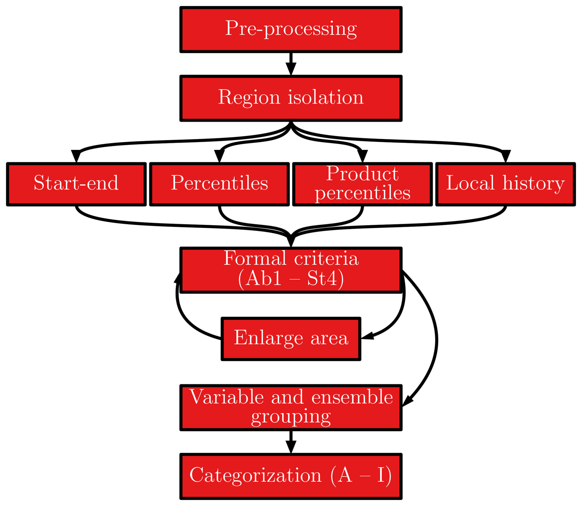
Figure 1The workflow that leads to SNS identification. At the first phase, monthly CMIP6 data is pre-processed by calculating annual means and regridding any of the original coordinate systems to a gaussian N90 grid. At the next step, promising regions are isolated based on four algorithms (see text), which are subsequently evaluated using formal criteria to identify the regions with an SNS. Regions where an SNS occurs are enlarged by merging with adjacent or overlapping regions or groups of 5°×5° square regions. Finally, we first group the SNS by combining ensemble-members and variables of one model that occur in overlapping regions and then manually categorize these SNS into 11 categories.
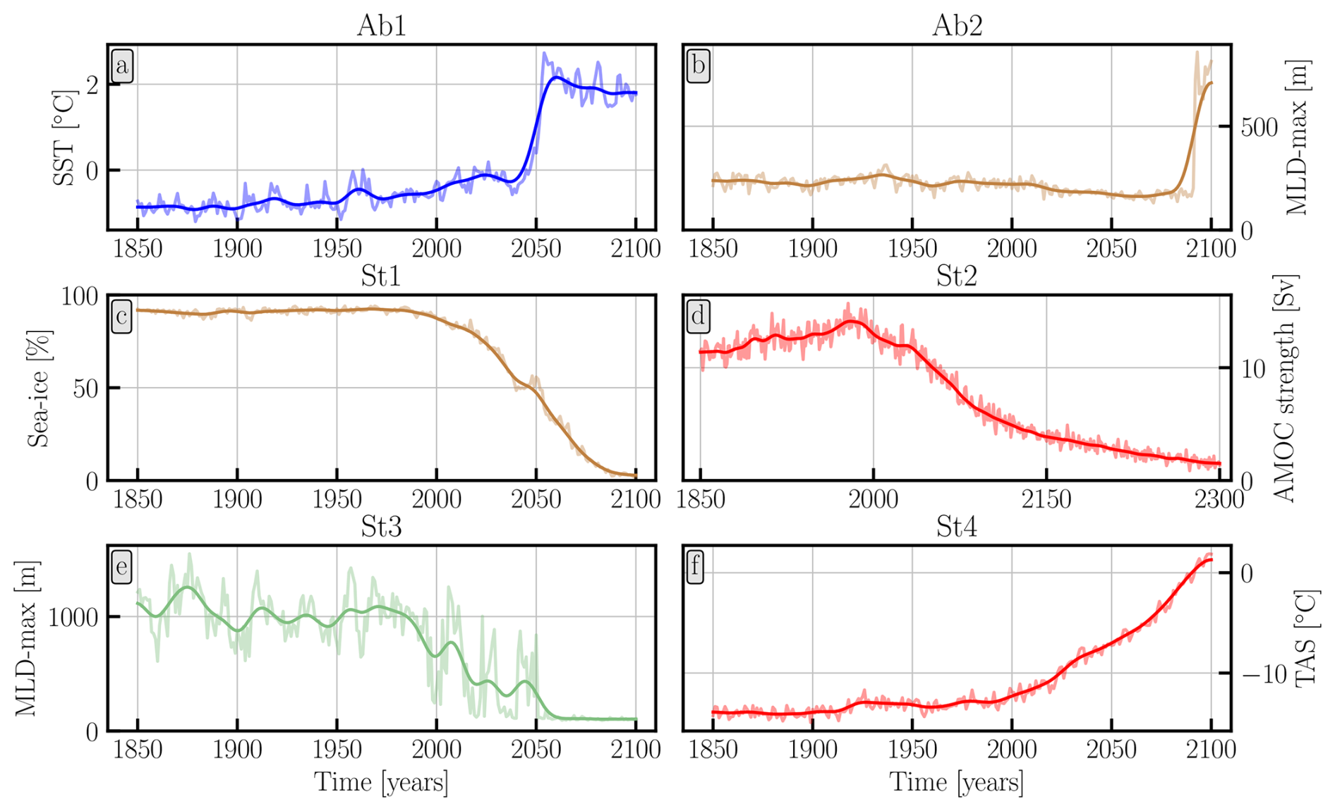
Figure 2Examples of the six formal classification criteria (Ab1-St4), see text for further details. Panels (a), (b), (c), (d), (e) and (f) refer to SNS 61, 60, 6, 50, 66, and 18 respectively in Table A3. The solid lines indicate the smoothed yearly time series (which are illustrated as shaded lines). The data is smoothed using a Lowess filter with a window of 40 years.
These strict requirements formalize the role of expert judgment of earlier work (Drijfhout et al., 2015). We used six different formal sets of criteria to detect various SNS events:
- Ab1:
Abrupt change.
- Ab2:
Abrupt change at the end of a dataset.
- St1:
Almost complete disappearance of sea-ice in an area of at least 5×10⁶ km2.
- St2:
Transition to an extremely weak state in the Atlantic meridional overturning circulation (AMOC)3.
- St3:
Transition from a deep to an extremely shallow ocean mixed-layer, or vice versa.
- St4:
Transition to a completely new state in other ocean/atmosphere variables.
An example of a time series associated with each criterion is shown in Fig. 2, and the definition of each criterion is discussed in the appendix (Sect. A2). The six different criteria-sets can be motivated by the moment the SNS occurs relative to the length of the time series and/or the nature of the climate system showing a state (phase) transition, the timescale of the inherent feedbacks, and the noise level of the system. We define two criteria related to abrupt changes; Ab1 and Ab2, where Ab2 is specifically developed for abrupt shifts at the end of a time series which implies that these SNS can never fulfil the demand of a bimodal distribution, otherwise applied. While having to relax this demand we somewhat sharpened other ones compared to Ab1 in the Ab2-set. We defined four different criteria-sets associated with state transitions. St4 is our standard set, applying to most ocean variables for which ocean dynamics and feedbacks dominate. St1 is developed for sea-ice and more specifically the disappearance of year-round (or winter) sea-ice in the Arctic. As this is a circumpolar phenomenon, we made the minimum area demand more stringent and demanded a 95 % decline of sea-ice in this enlarged area to exclude trivial sea-ice decline in a warmer world which occurs everywhere where sea-ice developed. For the AMOC we used a slightly different set (St2) as we deal here with a phenomenon that is integrated over depth and its zonal dimension, making it stand out from latitude-longitude patterns. For Mixed-layer depth we also adapted the criteria-set of St4 to the criteria-set St3 due to the much higher noise (variability) in its time series on the decadal timescales. The SNS we find with the criteria-set St3 would not have been isolated with St4 due to this higher variability. This adaptation was motivated by the large impact of atmospheric noise on mixed-layer depth and will be relevant for phenomena dominated by mixed-layer dynamics. For instance, this criteria-set will also be used for Ocean Biogeochemistry variables in a follow-up catalogue. Criteria-sets Ab1, Ab2 and St2 each detect several types of SNS (described below), while St1, St2, and St3 are each tailored to one specific type of SNS in this catalogue.
The criteria-sets Ab1, 2 and St1–4 have been formulated in such a general way that they cover all types of SNS that apply to mean states and are dominated by slow (order of ten years or more) processes relevant for the coupled ocean-sea-ice-atmosphere system. Other types of SNS events not considered here are changes in variability, extremes, and fast atmospheric dynamics. SNS events in hydrology, vegetation, carbon stores and ocean biogeochemistry will be discussed in a follow-up paper.
The equations related to each of the six sets of criteria are available in the appendix (Sect. A2). We have evaluated the formal criteria for each variable and each ensemble-member available in our dataset. In Table A2 we list all the investigated datasets. After combining ensemble-members, variables, and scenarios that overlap, we end up with 73 SNS, as will be discussed in Sect. 3. We group the 73 SNS into 11 categories (as in Table 1 and Fig. 16) by combining cases of different models that are in the same region and occur because of the same underlying physical processes. Another type of SNS is a possible cascade of tipping points. The possible occurrence of such interactions between tipping elements was recently discussed in Wunderling et al. (2024). If occurring within the timeline of CMIP6 simulations such cascades will implicitly be detected as our criteria-sets would detect both the primal tipping element and successive other tipping elements without explicitly making the link between the two. In our analysis we aim to identify cascades in SNS when they occur and discuss and table them as such later in this work.
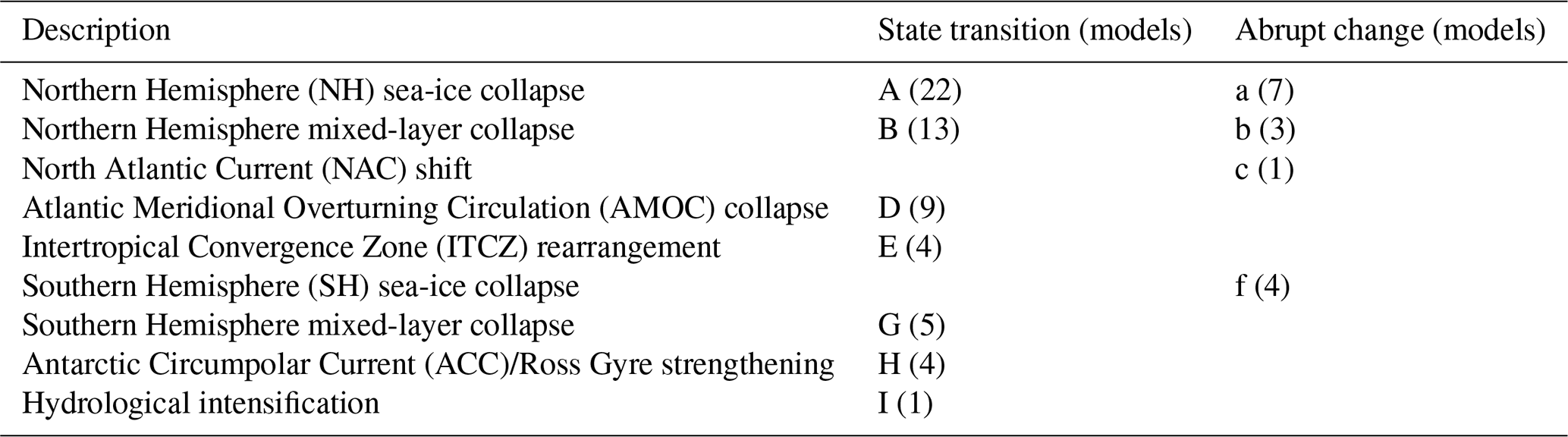
In theory abrupt changes and state (phase) transitions could coincide, making the distinction in the formal criteria (Ab1–St4, Sect. 2.3) look arbitrary. In practice, however, all abrupt changes involve a fast, nonlinear change in the state of the pertinent climate subsystem, that is too small to stand out as a state (phase) transition mainly caused by system feedbacks instead of a response to the forcing, while the state transitions that we do classify as such always evolve too gradual to classify as abrupt transitions. While this distinction often is a result of systems response to the different forcing applied in the various SSP scenarios and could be explained by strong local feedbacks in case of abrupt shifts and moderate forcing that do not upgrade to strong basin-scale or global feedbacks involved with a state transition in case of strong forcing, we will discuss them together but keep the distinction between the two. In total, we group the detected SNS into 11 categories (A–I), as given in Table 1. Some categories have related abrupt change and state transition SNS, for which we use the same uppercase letter for their state transitions and lowercase letters for abrupt changes to highlight their relation.
Table 1Categories of strong nonlinear surprises. For each category we label large state transitions with capital letters, while lowercase letters indicate abrupt changes. After each label, we denote the number of models that show that type of SNS between brackets. If a physical process causes both state transitions and abrupt changes in the same region, the same letter is used (e.g. A and a).
In the remaining sections, we discuss each of the 11 categories alphabetically (corresponding from North to South). For each category, we provide at least one exemplary case to demonstrate the related physical processes. However, categories may contain a multitude of models, SSPs, ensemble members, and variables. Demonstrating all possible permutations is beyond the scope of a single paper, we therefore provide the following additional resources and informational datasets:
-
Table A3 lists all cases, with categories, models, SSPs, variables and regions.
-
In Fig. A5, we show the first ensemble member for each SNS in each category, with each associated variable displayed independently.
-
Much information may still be outside the scope of this finite list of information sources, we therefore make the data relating to all cases available under (Angevaare and Drijfhout, 2025b). Here one can find a figure with isolated region and spatially averaged time series for each SNS, per model, per SSP-scenario, per variable, per ensemble member. Additionally, we also include the data for reproducing these figures and demonstrate how to extract several types of information from those data.
3.1 Abrupt year-round sea-ice loss in the Arctic (a) and transition to large, year-round ice-free areas in the Arctic (A)
3.1.1 Abrupt (Cat. a, 7 models)
As in Drijfhout et al. (2015), we find a few cases of abrupt sea-ice decrease in the Arctic. These cases are no longer restricted to the SSP585 scenario, as in CMIP5 for the RCP8.5 scenario, but also occur for weaker forced scenarios. Still, the forcing mechanism is in each case the global warming and polar amplification of this signal, mainly caused by the sea-ice albedo feedback (Davy and Griewank, 2023). In these cases the trajectories in the SSP126 and in the SSP245 scenario are qualitatively similar to the transition to a large, year-round ice-free area in the Arctic in the more strongly forced SSP370 and SSP585 scenarios. An example of this behaviour can be found in the CanESM5. Before 2050 the change proceeds abruptly but after 2050 it stabilizes unlike the evolution in the more strongly forced scenarios, which become part of Category A (transition to large, year-round ice-free areas in the Arctic, see also the difference between Figs. 3 and 4).
A qualitatively similar story holds for other models but depending on the model’s sea-ice sensitivity to global warming, abrupt changes may also occur for the SSP370 scenario. These cases are: CanESM5-1 (SSP119 and SSP245); EC_EARTH3-Veg-LR (SSP126); MIROC6 (SSP126, SSP245 and SSP370); and GISS-E2-1-H (SSP370). In one scenario the abrupt sea-ice loss induces equally abrupt changes in ocean and atmospheric variables, namely TAS (near-surface air temperature) in CanESM5-1 (SSP119).
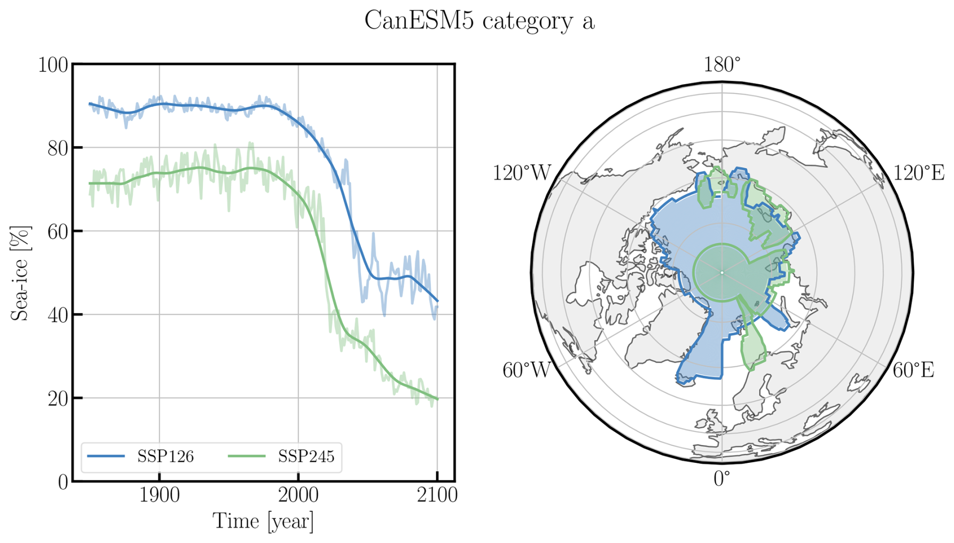
Figure 3Category “a” for the CanESM5 model (SSP126: r25i1p2f1, SSP245: r1i1p1f1). The left panel shows the yearly averaged time series (shaded) and the smoothed time series (solid), where we use the same smoothing as in Fig. 2. The right panel shows the corresponding region. This figure is one example of the category “a” abrupt changes, please see Table A3 for all models, as well as (Angevaare and Drijfhout, 2025b) for a complete overview with time series and locations for all SNS from all categories.
The relevant feedback mechanisms were already discussed in Drijfhout et al. (2015). This type of abrupt change was compared to the feedback-driven abrupt shifts in sea-ice edge found in an energy balance model (Rose and Marshall, 2009). This category's similarity to the state transition to ice-free conditions in more strongly forced scenarios (Sect. 3.1.2) points to anthropogenic warming as the driver, but internal variability may affect the timing of the abrupt event. Hankel and Tziperman (2023) demonstrated the existence of a winter (and thus year-round) sea-ice tipping point in a state-of-the-art climate model. In a previous study (Hankel and Tziperman, 2021) they identified a positive feedback cycle associated with this tipping point in which, at the start of winter, more open ocean water allows for moistening and warming of the lower atmosphere, which in turn increases downward longwave radiation, which reduces ocean freezing. The diminished winter sea-ice growth results in lower surface albedo, leading to increased shortwave absorption during springtime. In addition, increased ocean heat uptake causes even warmer ocean conditions that lead to further sea-ice reduction. Abrupt loss of Arctic sea-ice could also be driven by other positive feedback mechanisms (Abbot et al., 2009; Kay et al., 2012; Feldl et al., 2020)).
Large changes in sea ice that themselves do not classify as an SNS can trigger an SNS in ocean or atmospheric variables. One such example is the very large surface air temperature increase over the Pacific sector of the Arctic in UKESM-0-LL in its SSP126 scenario, which appears driven by sea-ice loss over that area allowing for atmospheric warming due to enhanced ocean heat loss (not shown). The sea-ice area involved is too small to classify as a category A transition and the change in sea-ice is not abrupt enough in sea-ice cover either, yet still causes an abrupt change in air temperature. This is an example of a cascade, not between tipping points themselves but between different variables associated with the same tipping event. Here, disappearance of sea-ice drives large and abrupt changes in the ocean-atmosphere interface. In this case sea-ice loss cascades into abrupt surface temperature increases.
Another such example is the abrupt increase in mixed-layer depth after the disappearance of sea-ice leading to enhanced heat loss from the ocean. This occurs in the Arctic where the yearly averaged mixed-layer depth increases from 50 to 350 m (CNRM-ESM2-1 in SSP245), north of 80° N and ranging from 10–120° E, roughly north of the Barents and Laptev Seas.
3.1.2 State Transitions (Cat. A, 22 models)
In Drijfhout et al. (2015) five models were found in which the winter sea-ice cover (siconc) largely collapsed. In CMIP6 many more of such cases appear, namely in 21 models and 29 model runs (ACCESS-CM2, ACCESS-ESM1, CanESM5, CanESM5-1, CanESM5-CanOE, CESM2-WACCM, CMCC-CM2, CMCC-ESM2, E3SM-1-0, E3SM-1-1, E3SM-1-1-ECA, EC-Earth3-Veg, FIO-ESM-2-0, GISS-E2-1-H, HadGEM3-GC31-LL, HadGEM3-GC31-MM, IPSL-CM6A-LR, MRI-ESM2-0, NorESM2-MM, UKESM1-0-LL, UKESM1-1-LL), although it should be noted that we focus on annual mean siconc and allow for arbitrary areas of more than five million square kilometres, rather than restricting the analysis to the entire Arctic north of 75° N as in Drijfhout et al. (2015). An illustration of this type of SNS in CMIP6 is given by Fig. 4. In Drijfhout et al. (2015) the Arctic winter siconc collapse only occurred in RCP8.5 extended runs. A model-dependent temperature threshold varying between 4.5 and 8.2 °C was needed for the onset of the winter siconc collapse. Such thresholds are much earlier reached in CMIP6 models (2.5–4.1 °C 68 % confidence interval, see Table 2 and Sect. 3.10).
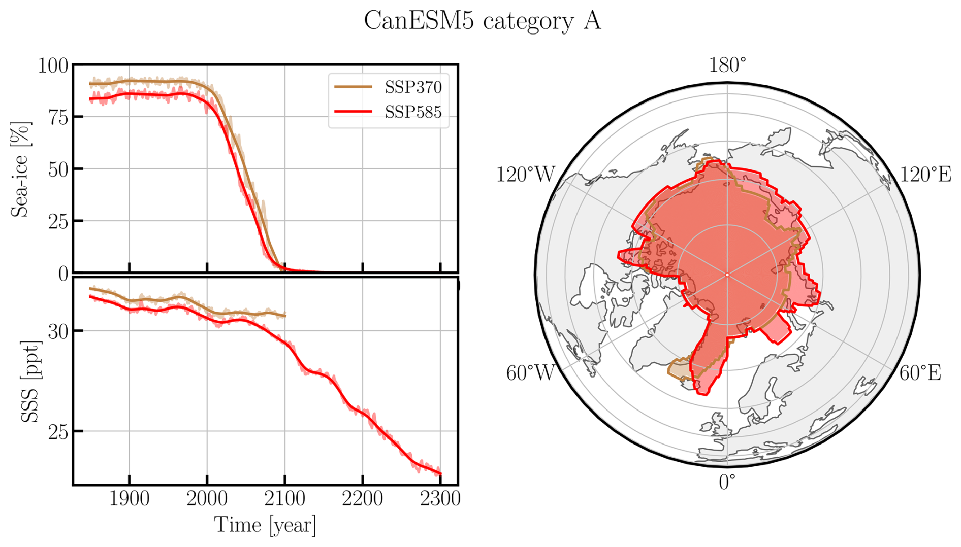
Figure 4Category “A” for the CanESM5 model (r1i1p1f1), where the SSP370 model run was evaluated until the year 2100 and SSP585 was extended to 2300. The sea surface salinity (SSS) is expressed in parts per thousand (ppt). The region (right) corresponds to the region wherein the sea-ice SNS is found, and, for consistency, the left panels correspond to these regions. For SSP585, an SNS was also found in a (smaller) sub-region for SSS. See caption of Fig. 3 for details.
Likewise as for some of the abrupt cases large-scale sea-ice loss cascades into state transitions for variables affected by enhanced ocean-atmosphere exchange. In these cases, the disappearance of sea-ice allows for a much stronger ocean-atmosphere coupling with enhanced heat and freshwater exchange that was otherwise shielded by the sea-ice lid and that now ultimately leads to a new ocean and/or atmospheric climate in the Arctic. Most of these cases are state transitions in sea surface salinity and atmospheric surface temperature, and sometimes circulation changes exemplified by state transition in sea surface height. They appear in SSP585 scenarios in ACCESS-CM2 (sea surface salinity; SSS), ACCESS-ESM1-5 (near surface air temperature; TAS), CanESM5 (SSS) see also Fig. 4, CESM2-WACCM (SSS and Sea Surface Height; SSH), FIO-ESM-2-0 (TAS), GISS-E2-1-H (SSS), MIROC6 (TAS) MRI-ESM2-0 (SSS), UKESM1-0-LL (TAS), and UKESM1-1-LL (TAS).
3.2 Abrupt Northern Hemisphere winter mixed-layer weakening (b), and State transitions to extremely shallow Northern mixed-layers (B)
3.2.1 Abrupt (Cat. b, 3 models)
In Drijfhout et al. (2015) several cases of abrupt change in Northern Hemisphere deep convection were identified. These were all cases where deep convection and mixed-layer depths collapsed. In CMIP6 we do not find any such case. This is in apparent contradiction with Swingedouw et al. (2021) who identified three CMIP6 models in which abrupt cooling events and abrupt transitions to very low mixed-layer depths in the North Atlantic subpolar gyre (SPG) occurred. Here, we do not classify those events as abrupt changes, as such changes are ubiquitous in the time series, also occurring in the historical and pi-control runs preceding the abrupt events that in Swingedouw et al. (2021) were identified (see their Figs. 1 and 6). This is partly due to the more stringent classification criteria we apply, among others by also comparing with the variability in the historical and pi-control runs, and due to the very large internal variability in mixed-layer depth, making it difficult for mixed-layer changes to classify as abrupt. Also note that Swingedouw et al. (2021) classified their abrupt events by demanding the associated temperature change to exceed a certain threshold. This discrepancy should not be interpreted that either we or Swingedouw et al. (2021) are right or wrong, but simply that what one finds as an abrupt shift depends on the criteria applied, and unfortunately, the criteria for an abrupt shift or SNS will always remain somewhat subjective, as for instance for what is coined extreme weather.
While we do not find abrupt changes in mixed-layer depth, we do find in three models abrupt changes in the North Atlantic SPG in ocean variables which concur with a significant, but non-abrupt mixed-layer depth decrease. These occur in scenarios SSP245 and SSP370 for cases where the decrease in mixed-layer depth in the SSP585 scenario over the same region is large enough to classify as a State Transition (category B). For this reason we include them in this section. In GISS-E2-1-G the abrupt change occurs for sea surface salinity (SSS) in SSP245 and SSP370, and for sea-surface temperature (SST) in SSP370 only; Fig. 5. Since both SSS and SST decrease, the driver for the mixed-layer decrease must come from SSS decreasing the surface density as freshening, only partly counteracted by the cooling that increases the surface density. This is again an example of a cascade of SNS variables in the same tipping point case, but now the large decrease in SSS is triggering a mixed-layer collapse, see also Drijfhout et al. (2025). Similar mixed-layer decrease-induced abrupt changes in ocean variables occur for GISS-E2-1-H and for CESM2-WACCM (SSS in SSP585).
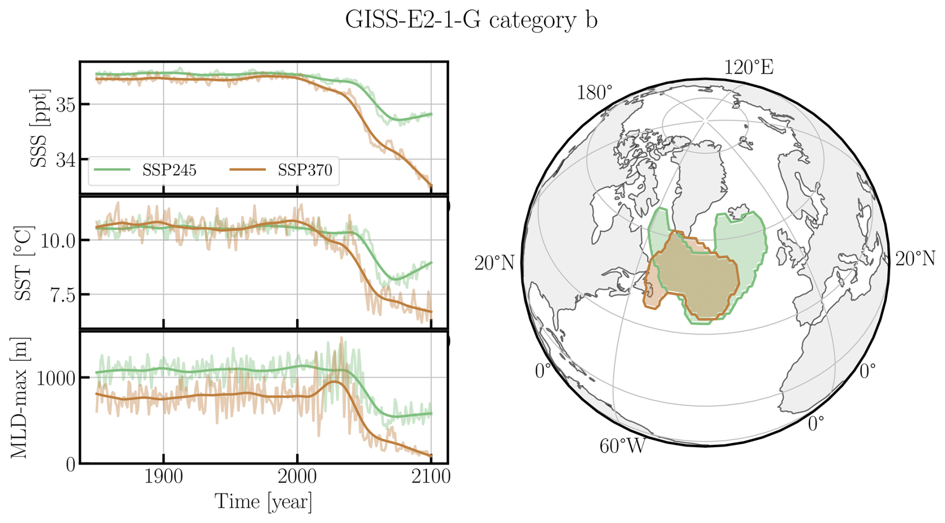
Figure 5Category “b” for the GISS-E2-1-G model (SSP245: r2i1p5f1, SSP370: r4i1p5f1). The SSP245 region belongs to the SNS detected in SSS, while the SNS for the SSP370 region is detected in SST. See caption of Fig. 3 for details.
3.2.2 State Transitions (Cat. B, 13 models)
While we do not find abrupt changes in mixed-layer depth, various models do show significant transitions from deep convection in the SPG to a state of no deep convection. This becomes more evident when data after year 2100 is included in the analysis. In our analysis, 10 models are identified featuring a collapse in mixed-layer depth in the Atlantic SPG and/or Nordic Seas. These are ACCESS-CM2, ACCESS-ESM1-5, CESM2, CESM2-WACCM, GISS-E2-1-G, GISS-E2-2-G, HadGEM3-GC31-MM, MRI-ESM2-0, NorESM2-MM, and UKESM-0-LL.
For all of those models the collapse occurs in the SSP585 scenario, but for CESM2 and MRI-ESM2-0, it also occurs in the SSP126, SSP245, and SSP370 scenarios; in CESM2-WACCM also in all scenarios but the SSP370 scenario was not run there. Curiously, in the GISS-E2-2-G model, the collapse occurs only in the SSP126 and SSP245 scenarios. These dramatic shifts in mixed-layer depth are, due to our requirement that they occur over an area of at least 106 km2, more often occurring over larger areas than just the Labrador Sea; often over the whole SPG and parts of the Greenland, Iceland and/or Norwegian Sea as well. In the UKESM-0-LL the collapse occurs in the Nordic Seas and develops between years 2020 and 2060; in the MRI-ESM2-0 and GISS-E2-1-G the collapse also includes the mixed-layer depth in Labrador and Irminger Seas. In the other models the collapse occurs in the Labrador and Irminger Seas only (e.g. Fig. 6). In all models the North Atlantic mixed-layer collapse occurs during the early to mid 21st century and often already starts around 2020. In Drijfhout et al. (2025), the collapse is analysed for the much smaller deep convection area and for the maximum mixed-layer (March) only, showing a far more abrupt signal with steepest decline around 2050. There, it is argued that the North Atlantic mixed-layer collapse precedes the AMOC collapse, and that this appears to be the main cause for the AMOC winding down to extremely weak states. As a result, this is a clear example of a tipping point cascade.
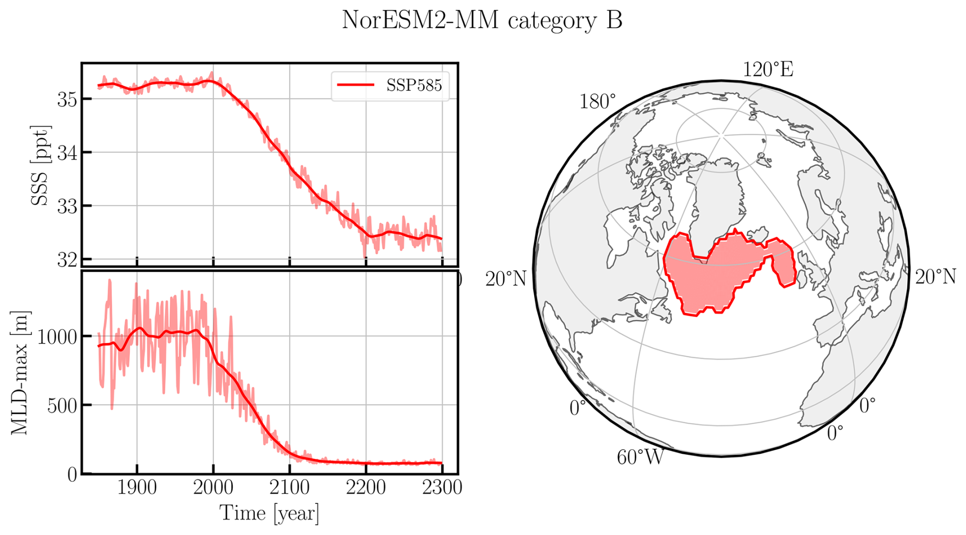
Figure 6Category “B” for the NorESM2-MM model (r1i1p1f1). The region (left) belongs to the region of the SNS detected in MLD-max. In this model run, the SSS also showed an SNS, that extended further in the Baffin Bay and less far eastwards. For consistency, the left panels correspond to the region in the right panel. See caption of Fig. 3 for details.
It should be noted that these collapses can occur in all SSP scenarios with an onset that sometimes already starts at a 1 °C warming level in the beginning of the 21st century, suggesting a strongly increased sensitivity in CMIP6 of mixed-layer depth and deep convection to global warming levels compared to CMIP5. Given the spread in warming level for the SPG- and Nordic Seas-convection collapse to occur, it is unlikely that global warming level is the right metric to measure its possible onset. As was already discussed in Drijfhout et al. (2015); Sgubin et al. (2017); Swingedouw et al. (2021), the onset of the collapse primarily occurs when the density stratification crosses a certain threshold, and this is more often caused by upper-layer freshening than by upper-layer warming, see also Drijfhout et al. (2025).
It should be noted however, that this freshening is brought about by a declining AMOC transporting less salty water northward, since increased meltwater release from a decreasing Greenland Ice Sheet was not included in CMIP6 simulations. A second mechanism causing the freshening is the convective feedback by which reduced mixing leads to fresher surface waters that further inhibit the vertical mixing (Kuhlbrodt et al., 2001). The trigger for AMOC decrease and freshening must come from the forcing and in these models is supplied by warming over the SPG reducing ocean heat loss and even reversing the sign of the surface heat flux in the SPG. The impact of decreasing surface heat loss to buoyancy gain, is however always smaller than the impact of freshening in terms of buoyancy at the surface, see Drijfhout et al. (2025) and van Westen et al. (2024) for more discussion on this topic.
In all models the mixed-layer collapse is associated with substantial freshening, but in some models this change in SSS even qualifies as a large state transition to much fresher surface waters. In ACCESS-CM2, CanESM5, NorESM-MM (as shown in Fig. 6) and UKESM1-0-LL this occurs in the Baffin Bay and Labrador Sea with sometimes an extension into the Hudson Bay and along the Labrador Current. Note that Fig. 6 nicely illustrates that although the mixed-layer collapse can ultimately be caused by salinity decrease it needs another trigger (i.e. changes in surface heat flux) as the start of the salinity decline lags the onset of the mixed-layer collapse. In CanESM5, the mixed-layer collapse itself does not qualify as an SNS, but the large-scale freshening in this region does. In GISS-E2-1-H and MRI-ESM2-0 the SSS transition occurs over the whole SPG and large parts of the Arctic. The freshening of the Arctic, however, must be associated with the melt and year-round disappearance of nearly all sea-ice there. In CESM2, the large-scale freshening occurs preferably in the eastern SPG.
3.3 Abrupt shift in the North Atlantic Current (Cat. c, 1 model)
Many low-resolution coupled models feature a strong cold bias east of Newfoundland due to an overly zonal North Atlantic Current (NAC) (Moreno-Chamarro et al., 2022). Associated with this bias in the current pathway a cold anomaly appears in sea-surface and surface atmospheric temperatures, which is often called the northwest corner bias. This bias is also present in the GISS-E2-1-H model, but surprisingly, NAC and surface temperatures feature an abrupt shift to a more northward pathway for the NAC through the central/eastern SPG, and subsequently warmer temperatures east of Newfoundland under the SSP119 scenario. The temperature change in the ocean is almost 3 °C and in the surface atmosphere over 2 °C, the upward heat flux doubles and sea surface height increases by almost half a meter. The change in SST is most abrupt, occurring within a decade around 2030 (Fig. 7). Why this change in NAC occurs most sharply in the SSP119 scenario in this model remains unclear, but it is remarkable that the bias can abruptly change in response to a modest increase in radiative forcing, much more than when that forcing becomes stronger in a higher-emission scenario. That the NAC can be steered by applying advanced forms of local flux correction was demonstrated by Drews et al. (2015), who argued that this also must be applied to the subsurface to adjust the flow field by modifying density and pressure gradients over a large vertical column. We hypothesize that in this model, perhaps by chance, the temperature and salinity adjustment in response to an SSP119 forcing conspire to change the pathway of the NAC. The GISS-E2-1-H model suggests the NAC can feature abrupt pathway changes that resemble a tipping point, but whether such a tipping point exists in nature remains unclear. Further investigation of this abrupt change, however, could be valuable in guiding bias reduction efforts in models with a northwest corner problem.
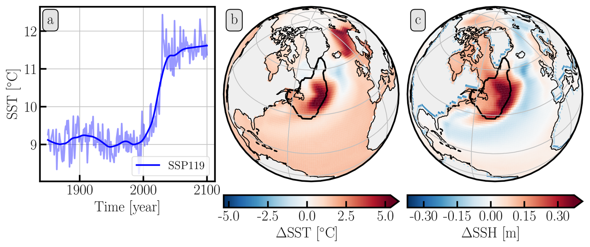
Figure 7The time series of SST for category “c” (panel a), together with the change in SST (panel b) and SSH (panel c) are shown for GISS-E2-1-H (r1i1p3f1). The change for SST and SSH is calculated between the averages for the 1850–1880 and 2070–2100 periods. The black outlined region in panels b and c illustrates the location of the SNS region. Since the global average SSH over time in GISS-E2-1-H does not equal zero (that would be the dynamical sea-level rise), we manually subtract the global average SSH from each year's data. The yearly data in panel a are illustrated by the shaded lines while the solid lines depict the smoothed time series, where the smoothing is the same as in Fig. 2.
3.4 Transition to extremely weak AMOC states (Cat. D, 9 models)
Given the widespread convection collapse in large parts of the northern North Atlantic in 10 models, it is unsurprising that an AMOC collapse also appears in seven of these and in two additional models. In the three runs in which the mixed-layer collapsed, but the AMOC did not, for one model (CESM2) the overturning streamfunction was not available, and for the other two models (GISS-E2-2-G and HadGEM3-GC31-MM) the respective runs stopped in year 2100, which is long enough to allow detection of a mixed-layer depth collapse, but too short to detect an AMOC collapse. Note however that in GISS-E2-2-G the AMOC declined in the 21st century from ∼25 to ∼12 Sv and in HadGEM3-GC31-MM from ∼18 to ∼7 Sv, implying that, were these runs extended to 2300, they probably would have shown a collapsed AMOC, almost certainly for HadGEM3-GC31-MM. Because an AMOC collapse tends to develop more slowly than the SPG convection collapse, it is most often identified in runs that were extended to year 2300 or beyond. These include the previously discussed models showing an accompanying mixed-layer depth collapse being the models ACCESS-CM2, ACCESS-ESM1-5, CESM2-WACCM, GISS-E2-1-G, MRI-ESM2-0, NorESM2-MM, and UKESM-0-LL. In all seven models the AMOC collapse occurs in extended SSP585 runs, but in CESM2-WACCM and MRI-ESM2-0 the collapse also occurs in the extended SSP126 runs. In addition, we identify an AMOC collapse in the CanESM5 and MIROC-ES2L in their SSP585 runs. For these two models the mixed-layer depth collapse was not observed. For MIROC-ES2L, the data was not available and in CanESM5 a mixed-layer collapse can be seen but did not qualify as a category B SNS because the mixed-layers in this model show a large decline everywhere in the ocean. In MIROC-ES2L, the AMOC collapse proceeds rapidly enough to be detected in a run that ends in year 2100. The onset of AMOC decline occurs in these models between years 1980 and 2020, corresponding to global warming levels between 1.0 and 1.5 °C, which is then completed between years 2150 and 2250 with an accelerated weakening until 2100–2150 and a slower approach to the new (quasi)-equilibrium. While a wind- and buoyancy-driven shallow overturning cell of ∼3 Sv always remains in these runs, the 5 Sverdrup (Sv) boundary is crossed between 2100 and 2140 in most models. Only in the CESM-WACCM model in the SSP126 scenario the AMOC stabilizes around 5 Sv.
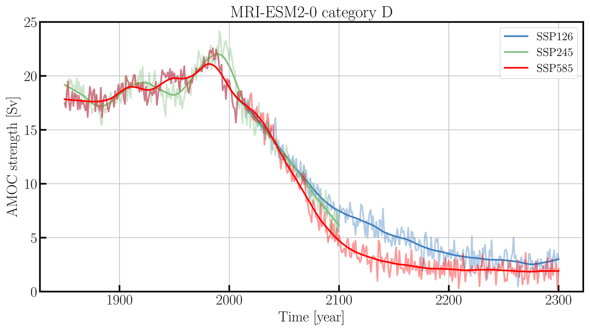
Figure 8Category “D” for the MRI-ESM2-0 model (SSP126: r1i1p1f1, SSP245: r4i1p1f1, SSP585: r1i1p1f1). The yearly data is illustrated by the shaded lines while the solid lines depict the smoothed time series, where the smoothing is the same as in Fig. 2.
In the MRI-ESM2 model the AMOC declines to ∼3 Sv in both SSP126, SSP245 and SSP585 scenarios, only a bit slower in the SSP126 and SSP245 scenarios. In this model the AMOC decline is similar in all scenarios until year 2050 (Fig. 8); in CESM2-WACCM even until year 2080. The AMOC collapse under an SSP126 scenario is a novel finding. It underscores the increased AMOC-sensitivity to warming in the multimodel mean Ensemble of CMIP6 compared to CMIP5 (see also Jesse et al., 2024 and Mecking and Drijfhout, 2023). It also suggests that in the MRI-ESM2 model the AMOC collapse can possibly be identified with a real tipping point as it largely becomes independent of the forcing and may already be committed to collapse decades earlier in the 21st century.
3.5 Transition to new ITCZ state (Cat. E, 4 models)
Large changes associated with a reorganization of the ITCZ are found in large-scale SSS transitions to much fresher surface waters in the western tropical Pacific in ACCESS-CM2, ACCESS-ESM1-5, CESM2-WACCM and IPSL-CM6A-LR. An example of this transition is given in Fig. 9. These changes occur exclusively in the SSP585 scenario and are associated with model bias. Many low-resolution coupled models feature a double ITCZ, especially over the Pacific Ocean (Moreno-Chamarro et al., 2022). This is also the case in the IPSL-CM6A-LR model and while the bias does not disappear in the SSP585 scenario, the signal over the equator, especially in the west Pacific, decreases abruptly. This is associated with a strong increase in rainfall over the region and reduced evaporation, caused by the double ITCZ becoming less pronounced. This change in ITCZ pattern causes a drop in salinity in the Pacific across the equator and most notably north of it, which occurs most abruptly along the western Pacific equatorial zone in one member4 of IPSL-CM6A-LR (Fig. 9). It is doubtful whether this change can be associated with a tipping point in the real world, as it originates from a strongly biased climate system, namely the double ITCZ, which is a common model bias, but not a feature of the real world (Tian and Dong, 2020). On the other hand, it is related to strong (positive) feedbacks between clouds, atmospheric convection and atmospheric/oceanic circulation that also are present in nature (Hwang and Frierson, 2013; Zhang et al., 2019). In principle, a large shift in the ITCZ could trigger (cascade) a Monsoon-related SNS (Geen et al., 2020). While we see a large increase in precipitation over the Himalayas, the area involved was too small to classify as an SNS in this model.
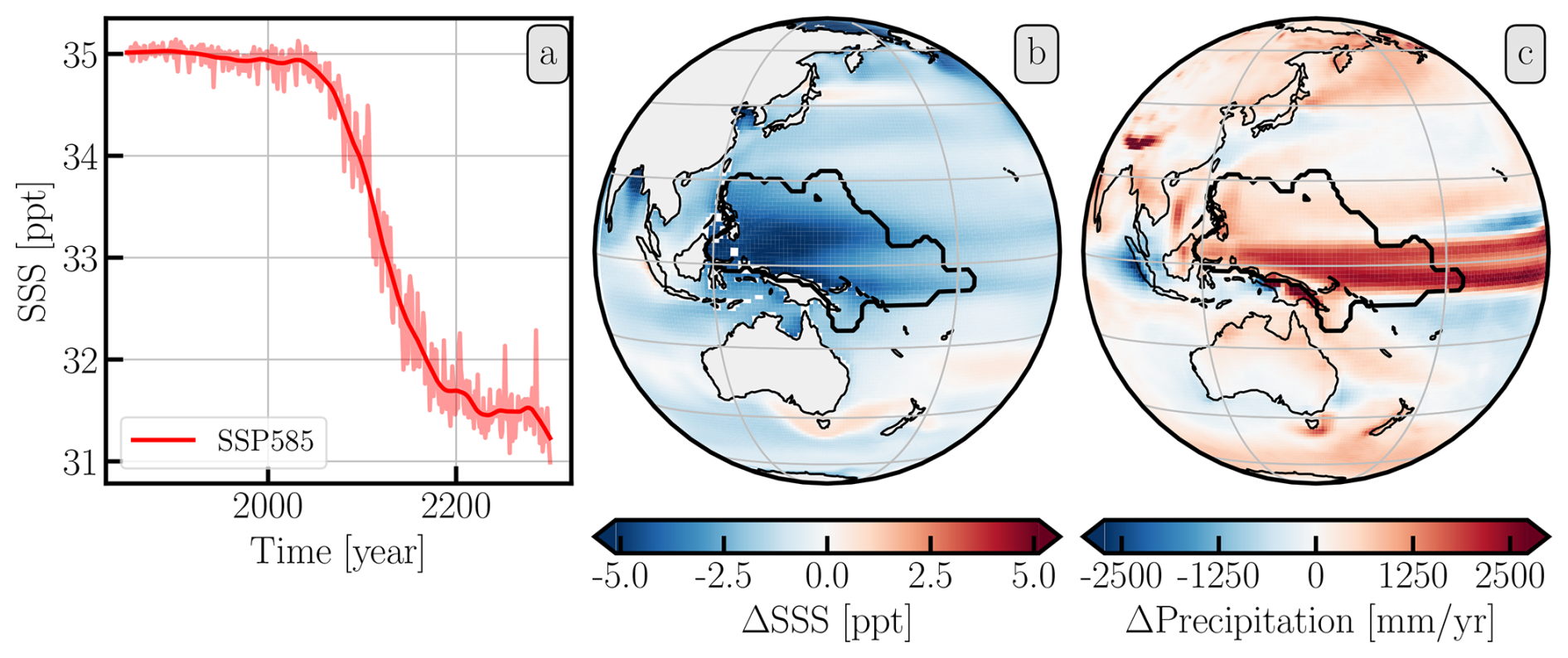
Figure 9The time series (panel a) of category “E” in IPSL-CM6A-LR (r1i1p1f1) is shown together with the change in SSS (panel b) and precipitation (panel c). The change for SSS and precipitation is calculated between the averages for the 1850–1880 and 2270–2300 periods. See the caption of Fig. 7 for further details.
3.6 Abrupt year-round sea-ice loss in the Southern Ocean, associated with abrupt change in ocean and atmospheric variables (Cat. f, 4 models)
We find four cases of abrupt sea-ice loss in the Southern Ocean. These cases are, like in the Arctic, probably triggered by warming of the overlying atmosphere, although the polar amplification/warming signal in the Southern Hemisphere is weaker. The abruptness of the event, however, needs strong nonlinear feedbacks from within the ocean and the most likely candidate is the onset of (deep) convection which, after the disappearance of sea ice, allows for large changes in surface heat flux. One such case was also found in Drijfhout et al. (2015) where the forcing mechanism resulting from the interaction of sea ice and deep convection was found similar to the one described in Lenderink and Haarsma (1996). The cases here can also be explained by the same mechanism. This interaction of feedbacks can only be triggered if the stratification under the sea ice is weak enough and therefore depends on subtle differences in the ocean mean state at the end of the historical period. Abrupt sea-ice loss in the eastern Ross Sea and Amundsen Sea occurs in the SSP585 scenario in HadGEM3-GC31-MM. Similar abrupt sea-ice loss, but more in the central Ross Sea, is seen in GISS-E2-1-H, accompanied with abrupt increases in upward heat flux and sea surface temperature for both the SSP245 and SSP370 scenarios, consistent with the onset of the deep convection mechanism that we propose. In the same model also an abrupt sea-ice loss occurs east of the Weddell Sea (Lazarev Sea) in most scenarios (SSP126, SSP245, SSP370, SSP585) which shows an almost complete collapse of perennial sea-ice there. Subsequent abrupt changes in the Lazarev Sea also occur for ocean and atmospheric temperature and surface heat flux (Fig. 10).
Depending on the variable, the abrupt change is seen in different scenarios; always in SSP126 but the change in SST is also abrupt in SSP245 and SSP370, and even in SSP119 where sea-ice itself disappears less abruptly. These changes all occur in the second half of the 21st century. A similar scenario for the Lazarev Sea occurs in CESM-WACCM, but the change in that model is only abrupt in sea-ice in the SSP585 scenario. This example illustrates that a fast, but non-abrupt change in sea-ice, can, if coupled to fast changes in convective mixing, trigger abrupt changes in ocean or atmospheric temperature.
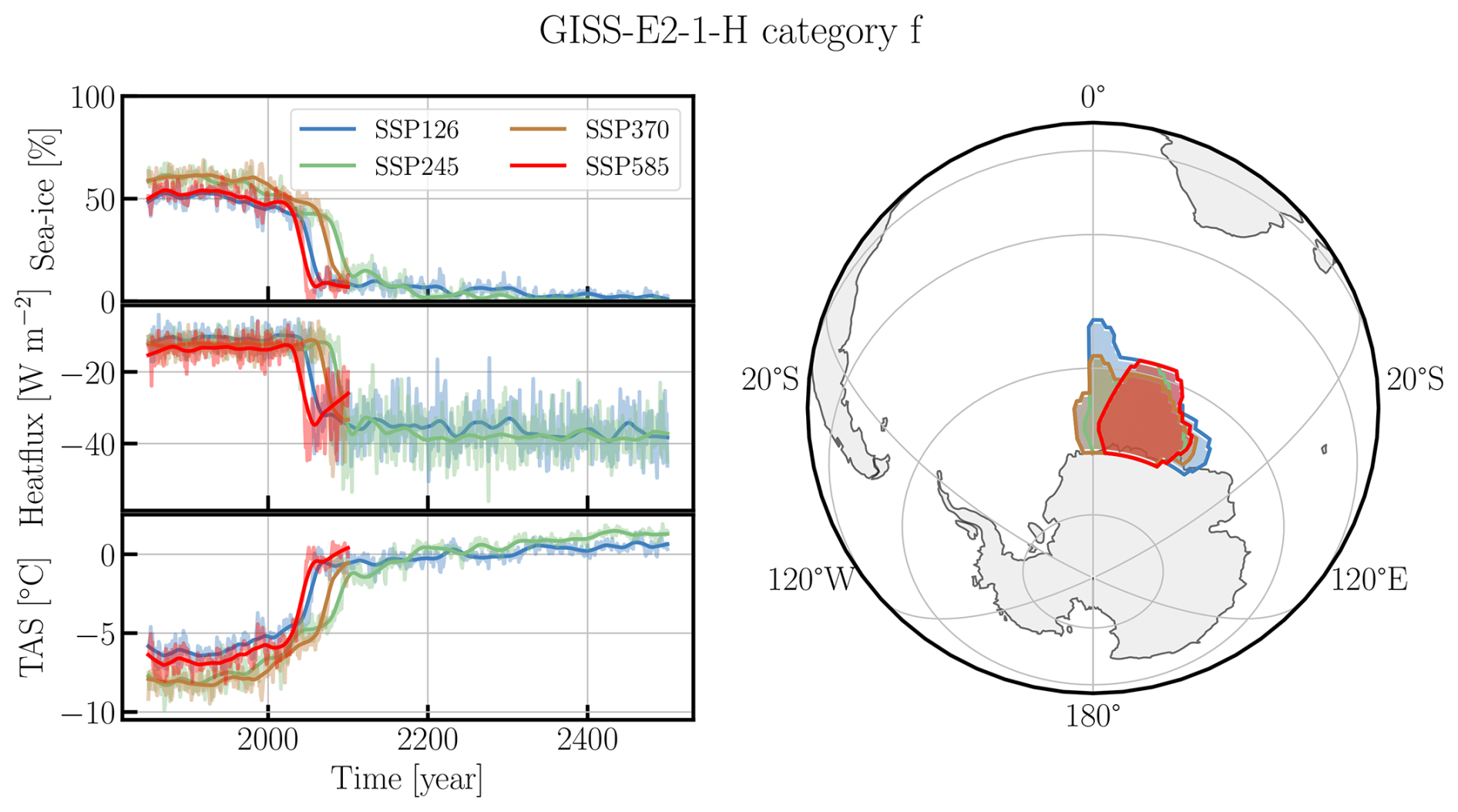
Figure 10Category “f” for the GISS-E2-1-H model (SSP126: r4i1p3f1, SSP245: r2i1p1f2, SSP370: r3i1p1f2, SSP585: r4i1p3f1). For consistency, the averages (left panels) are calculated over the region (right panel) wherein the sea-ice SNS are detected. See caption of Fig. 3 for details.
A similar scenario is simulated in the BCC-CSM2 model, but here we only see an abrupt change in mixed-layer depth without accompanying abrupt changes in other variables. The yearly averaged mixed-layer depth in the Ross Sea, in the middle of the Ross Gyre, suddenly increases from less than 100 to 1000 m between 2090 and 2095 in the SSP370 scenario. This abrupt change is associated with the disappearance of sea-ice, which itself does not occur abruptly. It should be noted that the feedback between sea-ice disappearance and the onset of deep convection associated with global warming has been demonstrated to occur for the Arctic (Våge et al., 2018), but not (yet) for the Southern Ocean. It should be noted, however, that this very same feedback was demonstrated to be instrumental in the multi-decadal variability in Southern Ocean sea-ice cover as sea-ice increase/decrease coincided with less or more deep mixed-layers Morioka et al. (2024). Instead of the increased warming resulting from SSP-scenarios these changes were triggered by the Southern Annular Mode, which, by changing upwelling of subsurface saline water, modulates the ocean stratification and can abruptly enhance or onset deep convection and subsequent sea-ice cover changes.
3.7 Transition to extremely shallow Southern Hemisphere winter mixed-layers (Cat. G, 5 models)
Mixed-layer collapses also occur in the Southern Hemisphere, but less often than in the Northern Hemisphere. We identified five such cases for different models (ACCESS-CM2, ACCESS-ESM1-5, CNRM-CM6-1, NorESM2-LM, NorESM2-MM). CNRM-CM6-1 shows a collapse in an atypical area: the Davis Sea in the Indian Ocean sector of the Southern Ocean. This site is not particularly known for deep convection and this SNS is therefore unrealistic and a result of model bias, although the type of SNS is in itself realistic, when occurring at other sites. The other models show a mixed-layer collapse in, or just east of the Weddell Sea. In ACCESS-ESM1-5, this occurs in the Lazarev Sea east of the Weddell Sea. In the other three models the Weddell Sea is the site where the mixed-layer collapse occurs (Fig. 11). As with the North Atlantic cases, these collapses all occur during the 21st century. Since open ocean convection in the Southern Ocean is a widespread feature of lower-resolution ocean and climate models, while in the observations, this type of deep convection is rare, and most of the Antarctic Bottom Water and its even denser precursors is formed on the Antarctic shelves, we do not assign much significance to these cases (Heuzé, 2021). The processes identified here, however, could be representative of the Weddell Polynya, where open ocean deep convection sometimes occurs, if it is opened (De Lavergne et al., 2014; Rheinlænder et al., 2021; Mchedlishvili et al., 2022). Anthropogenic-driven shifts in the Amundsen Low might play a role in causing abrupt changes on the Antarctic shelves, basal melt of the West Antarctic Ice Sheet and possibly the Antarctic Slope Current (Thompson et al., 2018), open ocean sea-ice and deep mixing (Holland et al., 2019; Drijfhout et al., 2024).
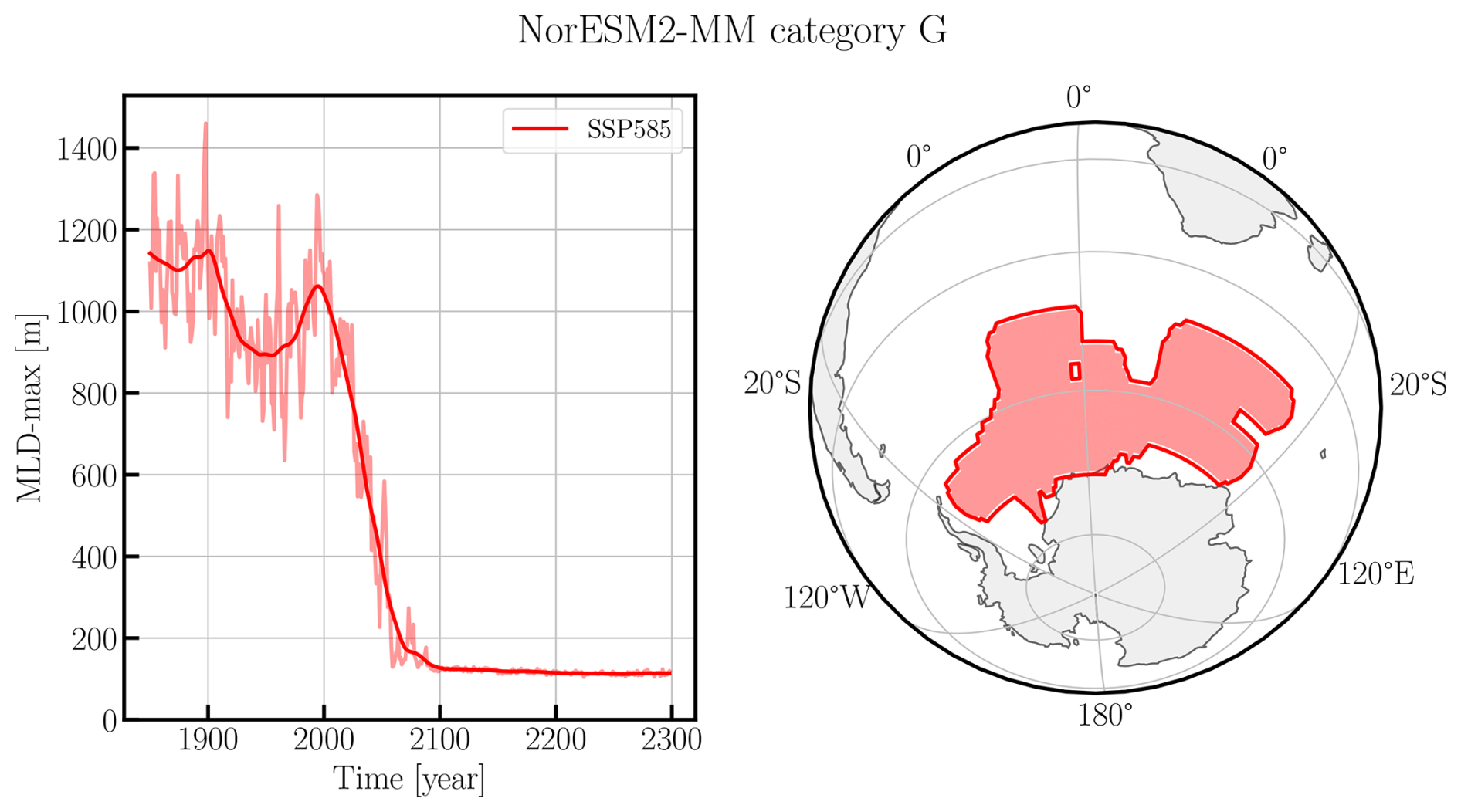
Figure 11Category “G” for the NorESM2-MM model (r1i1p1f1). See caption of Fig. 3 for details.
3.8 Transition to much increased Antarctic Circumpolar/Ross Gyre (Cat. H, 4 models)
Three models show a very strong drop in sea surface height (SSH) south of the Antarctic Circumpolar Current (ACC) associated with an increase in ACC mass transport of approximately 50 % in the SSP585 scenario (CESM2-WACCM, MRI-ESM2-0, UKESM1-0-LL). This is most likely related to the ACC response to the intensification of the Southern Hemisphere westerlies (Bracegirdle et al., 2013). This response, however, is probably spurious, in the sense that higher-resolution models show a much weaker ACC-sensitivity to winds, caused by what has been named eddy saturation (Munday et al., 2013), consisting of an intensification of the eddy field in response to increasing winds, rather than an increase in mean ACC transport. As a result, both SROCC (Meredith et al., 2019) and AR6 (Fox-Kemper et al., 2021) have assessed that the ACC is likely to remain only weakly sensitive to increasing winds. Moreover, such strong ACC response to winds may be enhanced by model bias explaining a large part of the spread in projections of CMIP5 models (Bracegirdle et al., 2013), which most likely also holds for CMIP6 models.
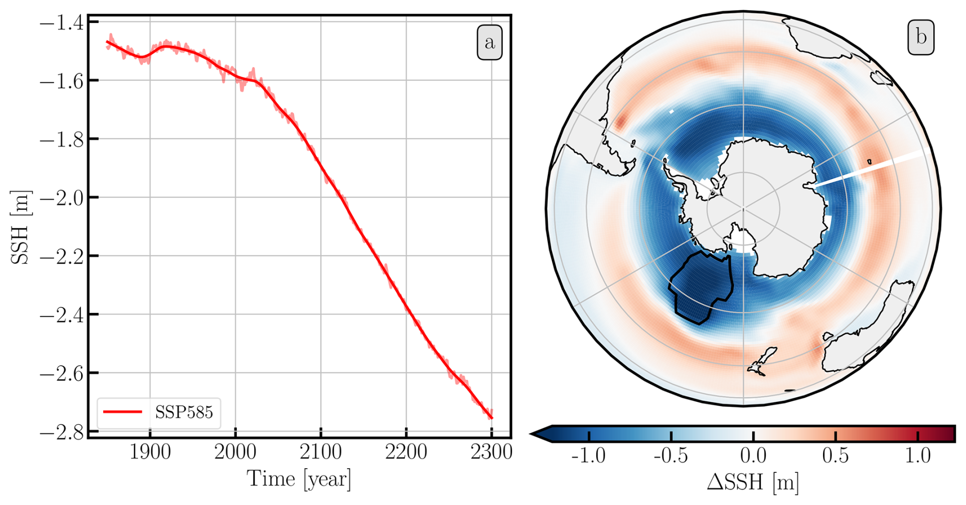
Figure 12Time series (panel a) of category “H” in IPSL-CM6A-LR (r1i1p1f1) together with the change in SSH (panel b). The change of SSH is calculated between the averages for the 1850–1880 and 2270–2300 periods. See the caption of Fig. 7 for further details.
One model (IPSL-CM6A-LR) shows a very strong drop in SSH just east of the Ross Gyre in the SSP585 scenario, associated with an 80 % increase in its regional depression. This is a sign of an eastward expansion of the Ross gyre, which also occurs in the UKESM1-0-LL (but less extreme than in IPSL-CM6A-LR), and was analysed by Gómez-Valdivia et al. (2023). They argued that sea-ice loss in the Amundsen-Bellingshausen sector enhances the wind stress curl on ocean water driving the eastward expansion of the Ross Gyre. This scenario was also described in a higher-resolution regional model of the region (Holland et al., 2019). Furthermore, the same process was already found to occur during the historical period (using an ensemble of high-resolution regional models forced with reanalysis data (Naughten et al., 2022)). As a result, this particular state transition is more credible than the projected increase in the ACC in some models.
IPSL-CM6A-LR also features a strong drop in SSH in other areas south of the ACC (Fig. 12), but here the circumpolar drop in SSH is slightly too small to classify the entire region as a state transition. The other models (CESM2-WACCM, MRI-ESM2-0, UKESM1-0-LL) that do identify the entire circumpolar region south of the ACC as a state transition in SSH show a less pronounced drop in SSH in the Ross Gyre than in IPSL-CM6A-LR. It is unclear whether the drop in SSH by the eastward extension of the Ross Gyre would classify as a state transition in a more realistic eddy-resolving model. In such a model, the ACC typically exhibits eddy saturation, and the circumpolar drop in SSH south of the ACC is either absent or remains modest (Stewart et al., 2023). Nevertheless, the response of the Ross Gyre appears robust and is corroborated in forced high-resolution ocean-sea-ice models.
3.9 State transition to much more humid climate over and in the Southern Ocean associated with strong intensification of the hydrological cycle (Cat. I, 1 model)
Another state transition is the large increase in surface freshwater flux in the Southern Ocean. This occurs in the CanESM5 model in the SSP585 scenario for the Amundsen-Bellingshausen sector (Fig. 13) and the wider Weddell gyre.
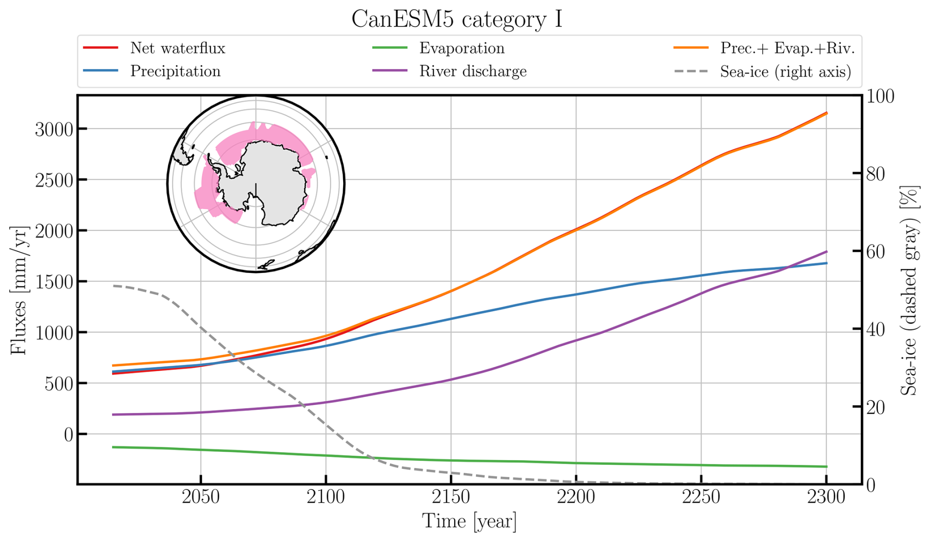
Figure 13Case “I” for the CanESM5 model (r1i1p1f1) as found in the net water flux, split by precipitation, evaporation and river discharge (purple). By summing (Prec. + Evap. + Riv.) the contributions of precipitation, evaporation, and river discharge we are able to close the water budget in this region. The right axis additionally shows the sea-ice cover in this region. The inset shows the region of the category I case in the CanESM5 model, where the region of the SNS is illustrated as the pink shaded region.
Although sea-ice cover dramatically decreases over these two areas, the increase in net water flux from atmosphere to ocean is not related to this (Fig. 13). It is shown that the increase in river run-off from the Antarctic continent (read snow melt and iceberg calving) plus precipitation (rain and snow) over the area (which also includes rain and snow over sea-ice) almost completely explains the increase in net water flux and when the increased evaporation (which acts as a negative contribution to this water flux) is included, the balance is closed. The reason for this large increase in water flux is thus the very strong increase in the hydrological cycle and transport of atmospheric water (vapor) from further north to Southern Hemisphere subpolar areas, in particular the eastern Pacific and western Atlantic sectors. It should be noted that CanESM5 features one of the highest Equilibrium Climate Sensitivities of CMIP6 (5.64 (Zelinka et al., 2020)), and as a result the intensification of the hydrological cycle is particularly strong in this model.
3.10 Global temperature rise at SNS
In the previous subsections, we discussed each of the 11 categories of SNS one by one. To see how often SNS occur in the available data, we first calculated the number of simulations that reach a given global warming level (since 1850–1880). To emphasize the contributions of the different SSPs, we considered each SSP for each model separately. That way, we have roughly 200 model-SSP combinations. Next, we needed to obtain the period in which each shift occurs. This is not always easily identifiable, for example panel c in Fig. 2 shows a sharp decline around year 2035, but also in year 2055, one might therefore argue that the SNS occurs at either of these years (and the temperatures associated with these years) or at a time in between these years.
To overcome this ambiguity, we used a flexible window w of 20–50 years to find the years (and the temperatures associated with them) at which the difference in w years in the w-year running mean is maximal, also see Sect. A4 for more information. The window w should be long enough to prevent measuring short term fluctuations as those apparent in panel (e) in Fig. 2, where before 1900 there are large, decadal time-scale changes (while the real change of interest evolves slowly in 2000–2050). The same window, on the other hand, should not be so long that it will span the entire scenario run duration since then all global warming temperatures will be associated with the SNS (such as Fig. 2 panel (a), which, using such a long window, always occurs in 2050). The flexible window w of 20–50 years strikes a balance between these two opposing interests and gives a PDF for the timing (and temperature) of maximum change.
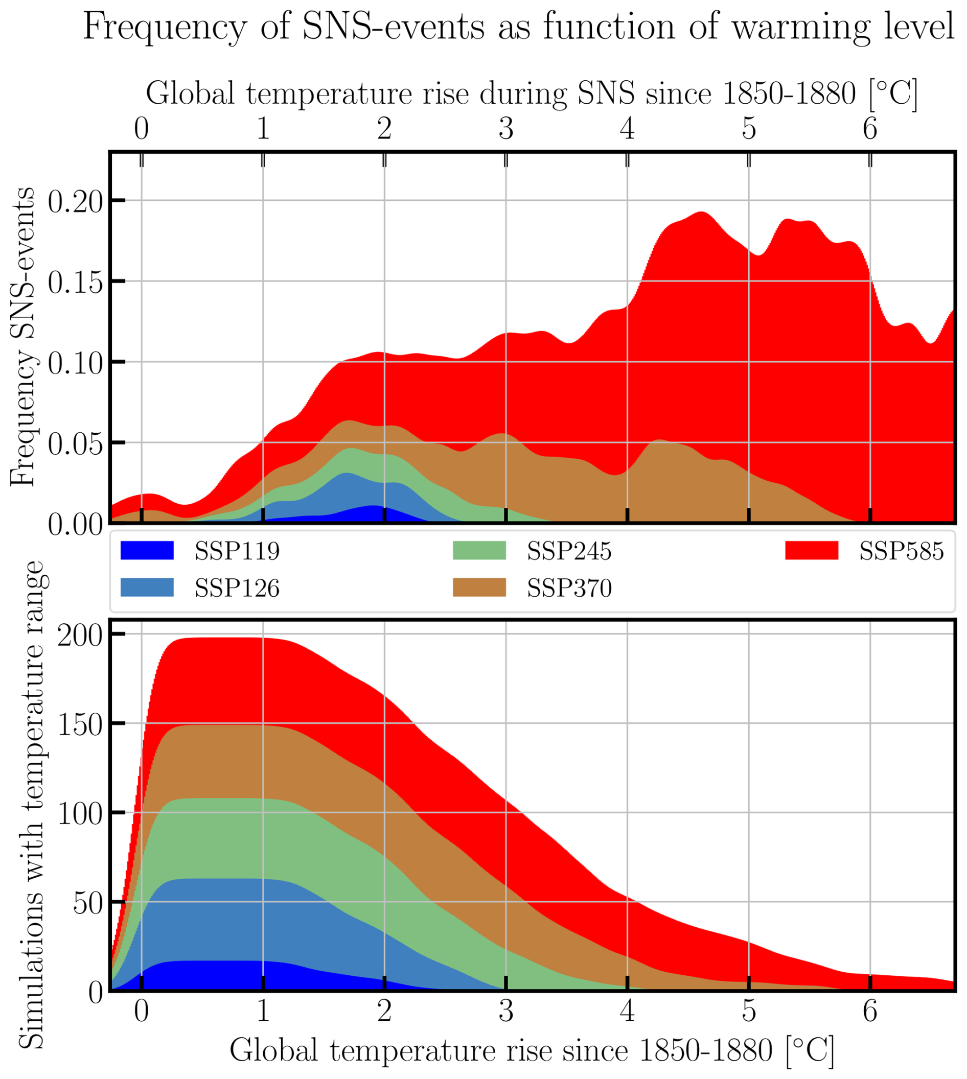
Figure 14Frequency of SNS (top) as a fraction of the number of available simulations that reach such a temperature range (bottom). The frequency of a shift is calculated by dividing the summed fractional probability of an SNS to occur in a temperature interval, divided by the number of available simulations that cover that interval (see text for details). The data is smoothed using a Gaussian convolution with a standard deviation of 0.1 °C. The temperature scale (x-axis) is limited to −0.3–6.7 °C, where at least five simulations are available (bottom panel).
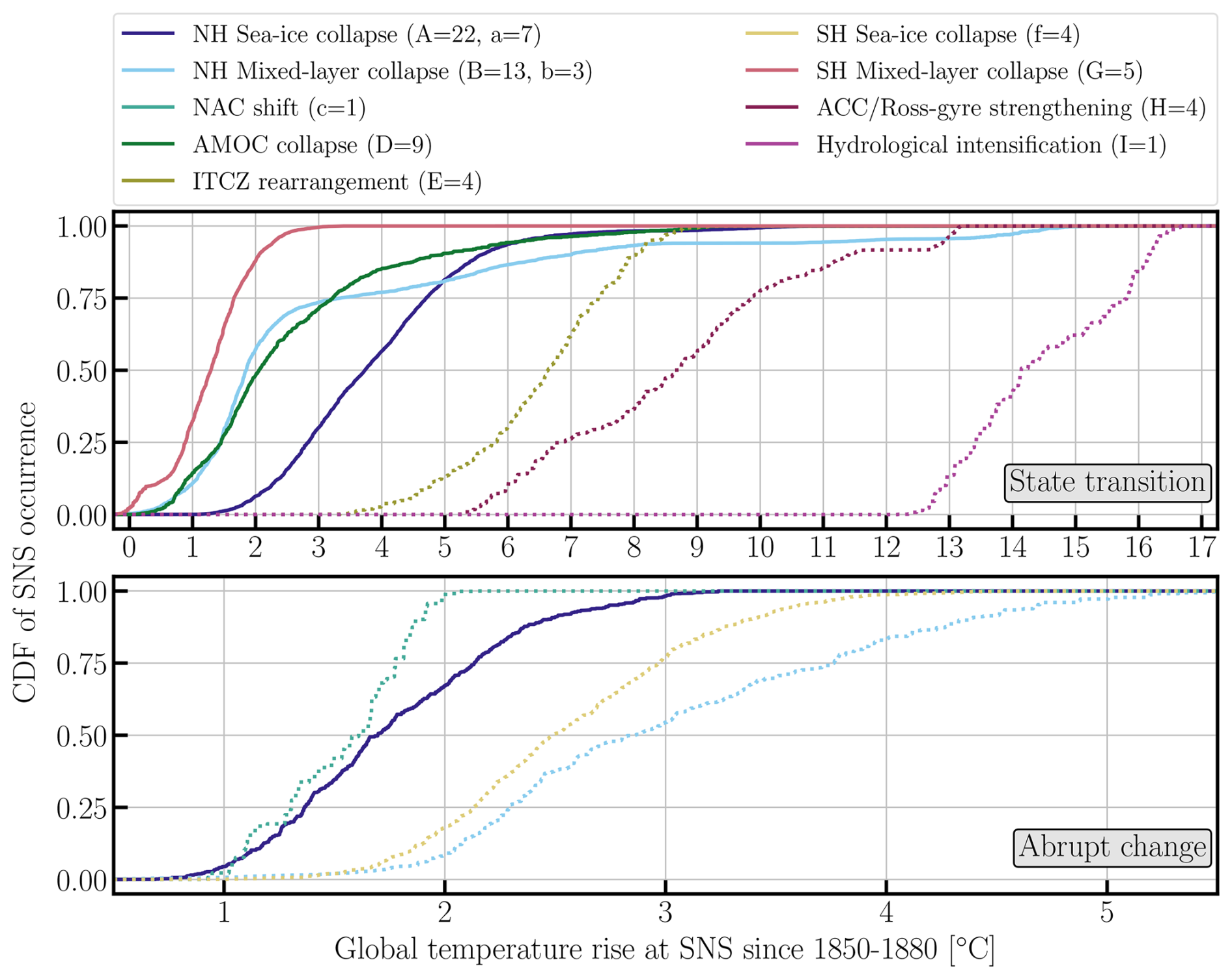
Figure 15Conditional CDF for SNS occurring per category as function of global warming level. The CDF quantifies the conditional probability that the change of the SNS is maximal (i.e. has a maximal derivative) at that global warming level, as explained in Sects. 3.10 and A4. The top panel gives the CDF for the state transitions (uppercase) categories while the bottom panel gives the CDF of the abrupt change SNS (lowercase) categories. The state transitions are often observed at (much) higher global warming levels, which therefore are displayed in a different global temperature rise range (x-axis) than the abrupt changes. The legend lists the number of models for each category. The categories that are observed for <5 models, have a higher uncertainty associated with their CDF (therefore displayed by dotted lines), compared to the categories with ≥5 models (solid lines).
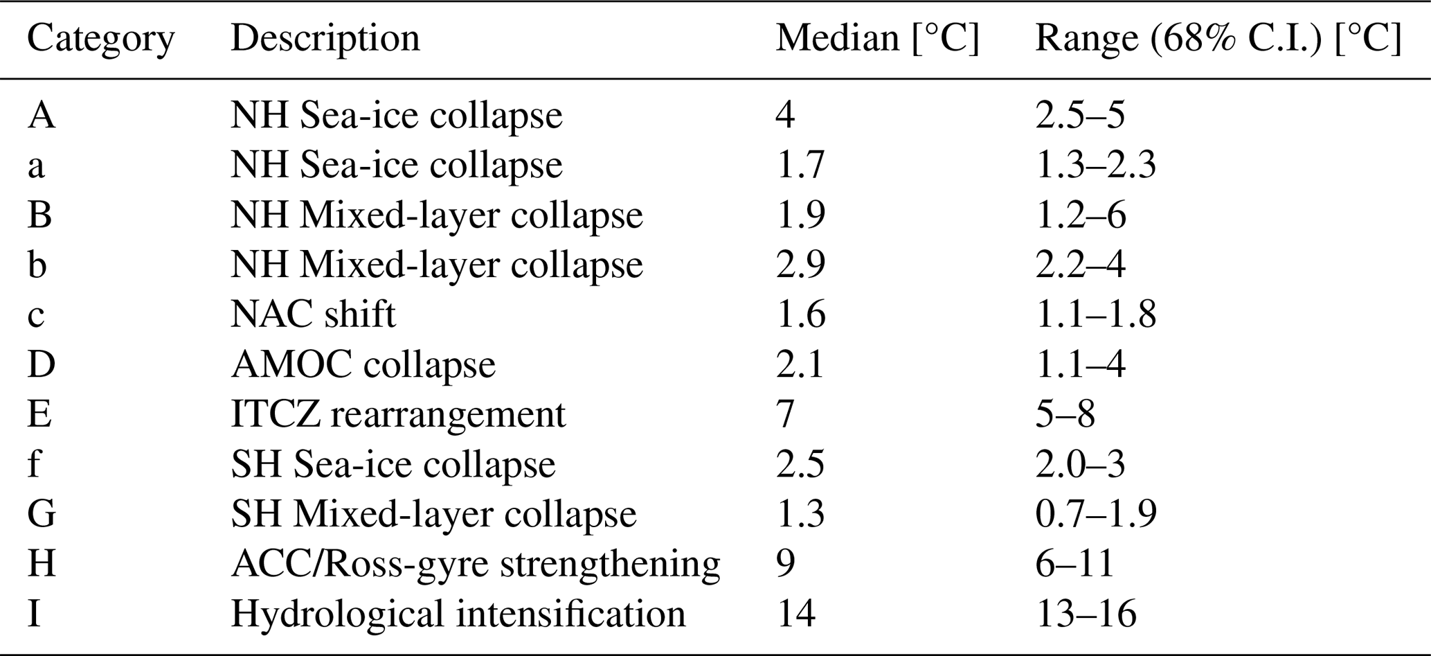
Table 2The global temperature identified for each SNS indicates the time at which the derivative is highest, as shown in Fig. 15. The median corresponds to 0.5 in Fig. 15, while the bounds of the 68 % confidence interval (C.I.) correspond to 0.16 and 0.84.
We then calculate the frequency at which temperature the SNS occur by summing the PDFs of all SNS and dividing that by the number of models that reach that global warming level. This leads to Fig. 14 where the bottom shows the number of available simulations for each temperature rise, while the top panel shows the frequency of SNS at each warming level. We normalize this distribution so that each change is accounted for once (even if it is observed in more than one variable). Additionally, models may have more than one ensemble-member, if this is the case, each of their temperature distributions is divided by the total number of ensemble-members. The top panel therefore shows (as a function of global temperature rise ΔT):
The frequency of SNS events (Fig. 14) increases steeply at global warming levels below 2 °C and remains relatively high between 2–4 °C. While the frequency of SNS rises further between 4–6 °C, this is based on a rapidly decreasing number of models (dropping from ∼ 54 to ∼ 10 in this interval), which correspondingly decreases the robustness of the inferred frequency. We should emphasize that Fig. 14 illustrates the warming level at which the changes in the SNS are maximal, meaning that the initialization of the SNS always precedes this time. If a tipping point is associated with the SNS, it is passed before the temperature noted here, when the transition to the new state is occurring.
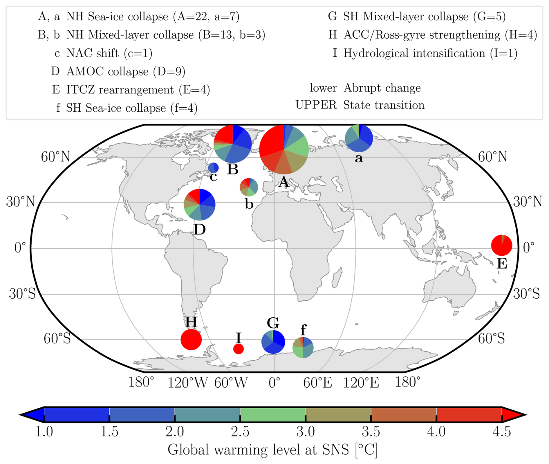
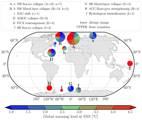
Figure 16Overview of SNS categories (Table 1). The pie-charts are scaled in size to the number of models in which the pertinent SNS are found (corresponding to Table A3). The associated colours show the average global warming level with respect to 1850–1880 using the method described in Sect. 3.10. The triangular extensions at the ends of the colour scale indicate out-of-range values: <1 °C at the lower end and >4.5 °C at the upper end. The locations of the pie-charts are indicative of the median location of the SNS within each category, which might be slightly shifted within the standard-error of latitude and longitude for illustration purposes.
We limit Fig. 14 to −0.3–6.7 °C global warming levels, where at least five simulations are available. The small, unexpected bump near 0 °C warming is an artifact (despite the method explained in Sect. A4) of the large maximum window size (50-years) that includes up to 25 years before (or after) the year of maximum change, combined with the very few simulations (bottom panel) that pass this temperature range.
We should note that the extended model runs (beyond the year 2100) are disproportionately represented in the SNS. The number of extended models (each normalized by the number of ensemble-members available to that model) compared to the total number of available models clearly illustrates this overrepresentation. The number of normalized extended models/number of available models is: 0.3/17 (2.0 %) for SSP119, 4.5/46 (10 %) for SSP126, 1.6/45 (3.6 %) for SSP245, 0.0/41 (0.0 %) for SSP370, 3.0/49 (6.2 %) for SSP585. The relative frequency of extended runs in those models that show an SNS is much higher: 0.0/2 (0.0 %) for SSP119, 5.0/10 (50 %) for SSP126, 1.8/10 (18 %) for SSP245, 1.0/16 (6.3 %) for SSP370, 7.0/26 (27 %) for SSP585. The larger availability of extended runs compared to Drijfhout et al. (2015) is one additional reason why the frequency of SNS is higher in our analysis.
In Fig. 15 we illustrate the CDF of the SNS occurring as a function of a global temperature rise. We see that the state transitions (uppercase SNS categories) generally occur at later timescales compared to the abrupt shifts. There are several reasons for this difference between the categories. As seen in e.g. Sect. 3.1, the change in sea-ice is sometimes observed as abrupt in the low-emission scenarios, while it is seen as a state transition in the high emission scenario where the disappearance of sea-ice is complete (see e.g. #6 and #27 in Table A3). Additionally, many state transitions are observed in the extended datasets. From Fig. 15, we can infer the temperature at which, for each category, the change in the SNS is maximal, which we include in Table 2.
Finally, we combine the spatial distribution and warming-level information for all SNS categories in Fig. 16. The position of each of the pie-charts in Fig. 16 is indicative of the mean global position of the SNS in that category. Each pie-chart indicates the global warming level at the time of the maximum change, we use the methodology above to build CDFs of the SNS-categories according to global warming levels. The pie-charts in Fig. 16 correspond to binning the probability of Fig. 15 between 1–4.5 °C global temperature rise, with overflow bins for SNS at global warming levels below 1 and above 4.5 °C. Figure 16 emphasizes the relative number of models that feature a certain category of SNS, as the size of each pie-chart is scaled to the number of SNS.
In this work, we have searched for SNS in CMIP6 data, focusing on ocean, sea-ice, and atmospheric variables. We identified 73 SNS that we grouped into 11 categories. Compared to Drijfhout et al. (2015), where 37 SNS were identified, this represents a large increase. It is unclear however, to what extent this increase is related to differences between CMIP5 and CMIP6 or due to our improved detection method.
The method used here made substantial changes to the approach discussed in Drijfhout et al. (2015). It allows for the isolation of arbitrarily shaped regions, while the region-selection in Drijfhout et al. (2015) was performed manually in rough 5°×5° rectangular longitude-latitude boxes and strict selection was already implied by the expert making the region-selection. In this work we now also rely more on formal, stringent criteria-sets and apply those to the arbitrarily shaped regions. Compared to the method used in Drijfhout et al. (2015) our method has become fully reproducible, as it no longer relies on expert judgment of time series.
In three cases we find it unlikely that the change in method can explain the increased numbers of SNS found here. Those are category A/a (Northern Hemisphere sea-ice collapse); category D (AMOC collapse), where we now find cases for lower emission scenarios as evident Drijfhout et al. (2015); and category B/b (Northern Hemisphere mixed-layer collapse). The increased number of SNS in these cases are due to a greater sensitivity of the AMOC to SSP scenarios than previously to RCP scenarios. Part of this may be explained by the larger climate sensitivity in some CMIP6 climate models (Zelinka et al., 2020), although, even corrected for this the AMOC remains more sensitive (Mecking and Drijfhout, 2023). Another reason is the possibly too large sensitivity to the (removal of) aerosol forcing (Menary et al., 2020) in a large suite of models, although this then also should apply to the mixed-layer collapse in the deep convection regions. We are nevertheless hesitant to argue that in CMIP6 AMOC sensitivity to changing forcing is too high. First no extra meltwater from a decreasing Greenland Ice Sheet is accounted for in CMIP6 models. In addition, models with less bias, in particular in the South Atlantic salinity structure, show stronger AMOC decline (Portmann et al., 2026). Note that these SNS events preferably show in model simulations extended to year 2300 or beyond, and that in CMIP5 fewer model runs were extended beyond year 2100. The larger number of SNS events in sea-ice collapse is also partly associated with the larger number of extended runs, but also to the decreased bias in sea-ice thickness over the historical period in CMIP6 (Notz and SIMIP Community, 2020).
We found abrupt changes and state transitions in 11 categories. For Arctic sea ice there is a clear shift of the onset of a year-round ice-free Arctic to lower temperature increases, implying this could occur already at the end of the 21st century. This shift is associated with a reduced bias in CMIP6 in sea-ice thickness in the historical period associated with a too cold Arctic, which we will elaborate on in a separate paper. A collapse of convective deep mixing also occurs faster and earlier in CMIP6 than in CMIP5 and may already develop between now and 2050, see also Drijfhout et al. (2025). One reason for this likely is a reduced stratification in the North Atlantic SPG. It is non-trivial to check the role of model bias for each individual case, but in general model bias is stronger in models not showing a collapse than in models showing a collapse, see Sgubin et al. (2017); Swingedouw et al. (2021). Associated with a mixed-layer collapse in all deep convective regions in the North Atlantic occurring earlier in CMIP6 than in CMIP5, also the AMOC features earlier shutdowns: a collapse of the North Atlantic Deep Water cell leaving a residual largely wind-driven overturning that does not extend northward of 30° N, see Drijfhout et al. (2025). In some cases, the shutdown even manifests itself in an SSP126 scenario, the scenario that fulfills the targets set in the Paris Agreement. Model spread in the AMOC response to global warming remains difficult to relate to model bias. One may argue that many models are too sensitive to aerosol forcing (Robson et al., 2022). This implies an AMOC decrease too strongly forced by aerosol removal since the nineties in the historical simulations and especially in the SSP126 scenario afterwards. On the other hand, it was recently shown that using observational constraints on model biases the AMOC decline in year 2100 became ∼70 % larger than using the unconstrained multi-model ensemble, implying that the better, less-biased models showed larger declines Portmann et al. (2026). Also, CMIP models do not include the freshwater flux from Greenland Ice Sheet melting and thus underestimate the freshwater forcing that enables an AMOC shutdown via increasing stratification in the North Atlantic SPG and inhibiting convective mixing there.
We also show that a shutdown of the AMOC is preceded by a collapse of deep mixing in the SPG (including the Nordic Seas, Drijfhout et al., 2025). This interaction between collapsing deep mixing and a collapsing AMOC is a clear example of cascading tipping points. The interaction between deep convection, regional sea-ice cover, air/sea fluxes and changes in ocean and atmospheric surface temperature sea surface salinity also shows elements of a cascade, but we would argue these are not separate tipping points but a cascade of tipping variables within a common tipping point/element.
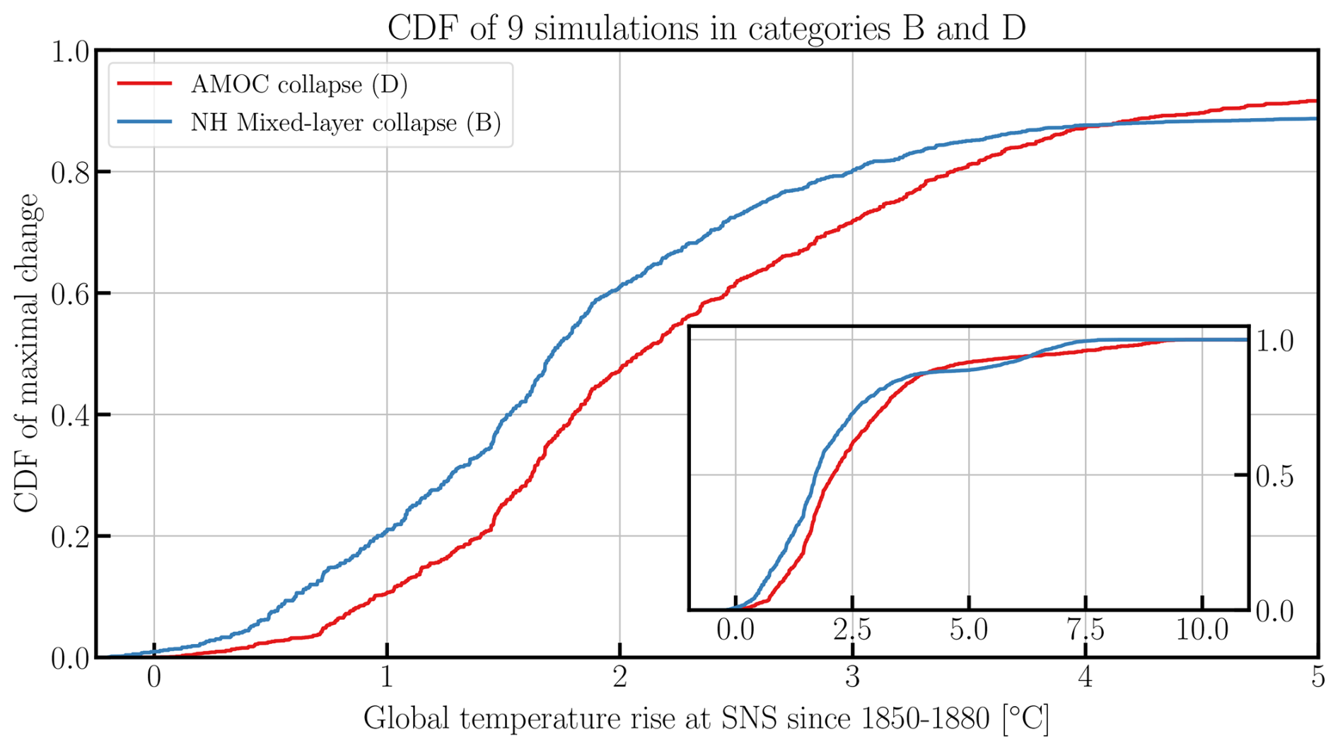
Figure 17The change in category B SNS precedes the change in category D SNS. We show this using the cumulative distribution function (CDF) of the change being maximal before a global temperature rise for nine model runs that are in category B and in category D. We select the nine simulations (ACCESS-CM2, ACCESS-ESM1-5, CESM2-WACCM, GISS-E2-1-G, MRI-ESM2-0 (SSP126 and SSP585), NorESM2-MM (SSP126 and SSP585), and UKESM1-0-LL) that have the same ensemble-member in both categories B and D. The main panel shows that the collapse of the mixed-layer depth occurs 0.3–0.4 °C before the collapse of the AMOC. The inset shows the CDF over the full temperature range. The approach to obtain this figure is similar to that of Fig. 14 (see text for details Sect. A4).
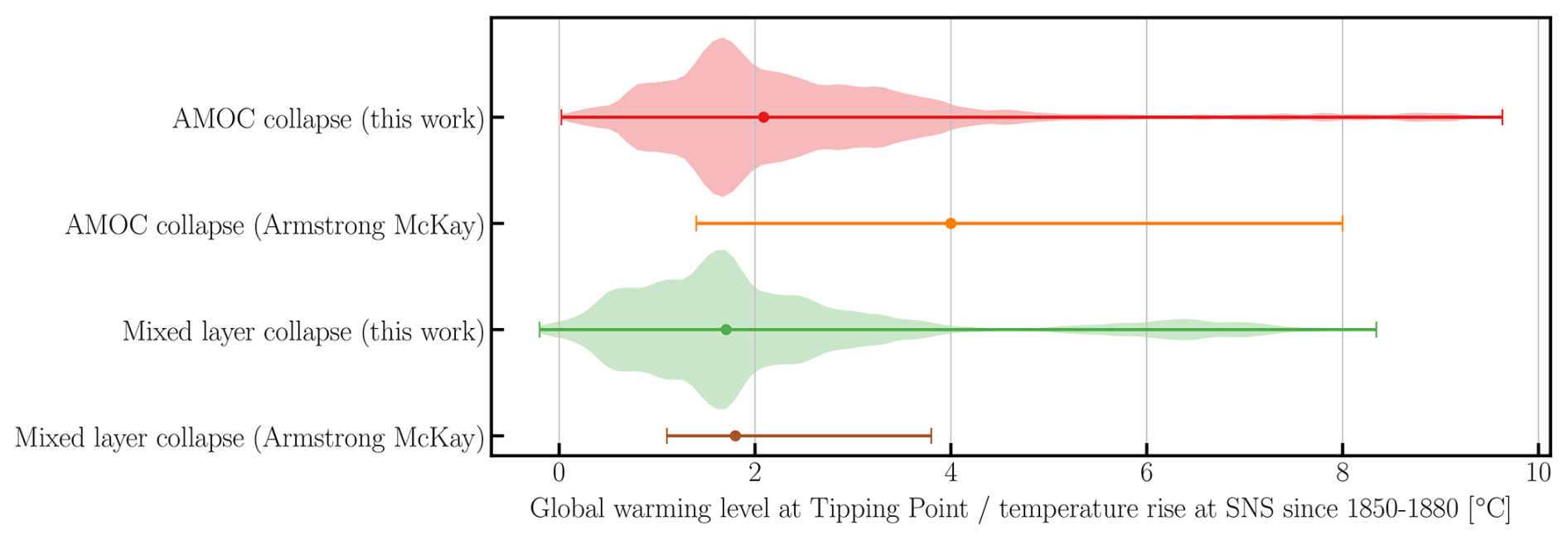
Figure 18Comparison of global warming levels thresholds for tipping points (Armstrong McKay et al., 2022) and the occurrence of maximal change of SNS (this work), where we compare the full CDF of Fig. 17 illustrated with violin plots, to the Min, Estimate, and Max global warming level thresholds described in Armstrong McKay et al. (2022). On top of the violin plots, we indicated the 0th-, 50th- (i.e. median), and 100th-percentiles of the CDFs with error bars. We compare our result AMOC collapse (Category D) to the Atlantic M.O. Circulation collapse, and our result NH Mixed-layer collapse to the Labrador-Irminger Seas/SPG Convection collapse. As discussed in the text, the metrics from Armstrong McKay et al. (2022) and this work are inherently different, and this comparison is therefore not one to one.
As discussed in Sect. 3.2.2, based on the findings in Drijfhout et al. (2025), a collapse of deep mixing in the Labrador, Irminger and Nordic Seas is found to precede a shutdown of the AMOC related to the formation of North Atlantic Deep Water in CMIP6 models. This is further illustrated by Fig. 17 where we see the Northern Hemisphere mixed-layer collapse to occur at 0.3–0.5 °C earlier which corresponds to ∼ 20–30 years earlier. For this reason, we argue this is a clear example of a tipping point cascade. In addition, this cascade also occurs earlier than previously estimated (Fox-Kemper et al., 2021; Armstrong McKay et al., 2022; Loriani et al., 2025) as illustrated by Fig. 18, which compares the models discussed in Sect. 3.4 using the methods from Sect. A4 to the result from Armstrong McKay et al. (2022). It should be noted that in Armstrong McKay et al. (2022) the given uncertainty range is based on the minimum and maximum global warming levels thresholds from expert judgment that is based on their estimate of being likely (together with the median). This is an inherently different approach to the CDF-based method of maximal change described above, making a one to one comparison infeasible. Fig. 18, together with Fig. 17 also supports that we see here a tipping point cascade between a mixed-layer collapse triggering the AMOC collapse in the models. After being triggered by atmospheric forcing (for example, due to global warming), further re-stratification of the water column becomes more determined by freshening brought about by a declining AMOC and even more by convective feedbacks resulting from reduced vertical mixing amplifying the reduction further (Drijfhout et al., 2025). This process also develops faster than the full AMOC shutdown and thus the SPG mixing collapse precedes the AMOC shutdown. However, for the AMOC collapse a mixed-layer collapse in all deep convective regions (including Nordic Seas) is needed (Drijfhout et al., 2025).
A few cases we found were clearly associated with model biases but still contained valuable information for more general tipping point behaviour of the pertinent climate subsystem and possible routes how to improve model bias. These examples were an abrupt shift in the North Atlantic Current in a model where its pathway was biased towards a more realistic pathway, a shift from a double ITCZ (model bias) to a more single ITCZ (realistic), large freshwater flux increases in parts of the Southern Ocean neighbouring the Antarctic continent in a model with an extremely high climate sensitivity and in an extended SSP585 simulation, abrupt changes in deep convection at places in the Southern Ocean where open ocean convection is not observed, and a strong response of the ACC to future increasing Southern Hemisphere winds, which is deemed unrealistic as CMIP models do not include the breaking of mesoscale eddies on such increase due to their coarse resolution. This underscores one of the main findings in a previous CMIP5 catalogue of SNS (Drijfhout et al., 2015), namely that many SNS appear stochastic and only occur in some models and/or even in some ensemble members of one model, implying that small changes in background state and/or atmospheric variability (noise) may determine whether an SNS occurs or not. A nice example of the stochastic bifurcation between a 10-member ensemble simulation featuring two members with an AMOC collapse and eight members in which the AMOC recovered under an SSP245 scenario illustrates this point (Romanou et al., 2023). This also implies that an SNS found in one or a few models may not have a counterpart in the present or future climate of our planet, but that we cannot rule this out unless the model at hand is severely biased and the SNS depends on this biased climate in a crucial way. This is probably true for the SNS associated with a shift in the North Atlantic Current and with a shift from a double to a single ITCZ in the tropical Pacific.
Some SNS in the Southern Ocean, although occurring in one or only a few model simulations, could be realistic and cannot be simply discarded as results from model bias. These are sudden disappearances of sea ice in regions where deep convection is triggered, a collapse of deep convection and mixed-layer depth in other Southern Ocean regions, and an eastward expansion and strengthening of the Ross gyre (Holland et al., 2019; Naughten et al., 2022). The first two types of SNS are associated with a well-known convection-sea ice interaction demonstrated to occur in the Arctic (in observations and in models), and playing a role in low-frequency changes in sea ice and mixed-layer depth in the Southern Ocean (Rheinlænder et al., 2021; Mchedlishvili et al., 2022), demonstrating the realism of the mechanism in the Southern Ocean as well. The eastward expansion of the Ross gyre is demonstrated in various eddy-resolving ocean-only models and is not affected by the inability to resolve eddies.
It is impossible to compare our results on a one-by-one basis with those obtained in Terpstra et al. (2025) who performed a somewhat similar but more restricted analysis as we have done here, also (partly) focusing on other variables than we do, but more importantly, analysing results from another scenario, namely the 1ptCO2 scenario, which starts in the preindustrial and increases every year with 1 % its CO2 concentration until the preindustrial value is doubled. What is immediately apparent, is that our and their approach both lead to the conclusion that in CMIP6 thresholds for abrupt shifts/SNS are earlier passed and at lower temperatures for all variables that we both analysed. In that respect our results confirm each other. In this work, we have focused on ocean, sea-ice, and atmospheric variables that are involved in the coupling to ocean and sea-ice changes. A logical next step would be the assessment of vegetation, carbon-cycle and related CMIP6 variables, as also Drijfhout et al. (2015) found a substantial number of SNS in this regime, as well as assessing SNS in fast atmospheric systems including extreme weather.
We have searched for SNS in CMIP6 data, with a focus on ocean, sea-ice, and atmospheric variables. We aimed to identify both abrupt changes over a decadal timescale and more gradual state transitions too large to be explained by increasing forcing only. We isolated 73 SNS that we categorized in 11 categories, which we each discussed. Of the identified SNS, 45 % is attributed to sea-ice loss (categories A, a and f) related to sea-ice cover, 29 % to mixed-layer depth (categories B, b and G), 19 % to ocean currents (categories c, D and H), and 7 % to atmospheric systems like the Intertropical Convergence Zone (categories E and I). The frequency of SNS events increases steeply at global warming levels below 2 °C and remains relatively high between 2–4 °C. While the frequency of SNS rises further between 4–6 °C this is based on a rapidly decreasing number of models (dropping from ∼54 to ∼10 in this interval), which correspondingly decreases the robustness of the inferred frequency. In general, the CMIP6 data contain various SNS that occur at lower temperature increase and earlier in time than estimated in previous assessments of SNS (abrupt changes) and tipping points, pointing to an increased sensitivity of the newest generation of climate models to anthropogenic forcing and an increased risk to strong nonlinear surprises, especially those associated with Arctic sea ice, the AMOC and convective mixing in the North Atlantic SPG. This finding signifies a strong warning to limit further future global warming as much as possible.
A1 Region isolation example
In this section, we provide an example of the first region-isolation approach discussed in Sect. 2.2. The approach aims to select regions that have a high probability to fulfil any of the formal SNS criteria of Sect. 2.3. In this example we perform the region isolation for SSS, GISS-E2-1-G, SSP245 (ensemble r1i1p5f1), corresponding to case number #44 in Table A3. This example, as well as the other three region isolation approaches, is also available online (Angevaare, 2025a), specifically https://github.com/JoranAngevaare/optim_esm_tools/blob/master/notebooks/advanced_methods.ipynb (last access: 17 July 2026).
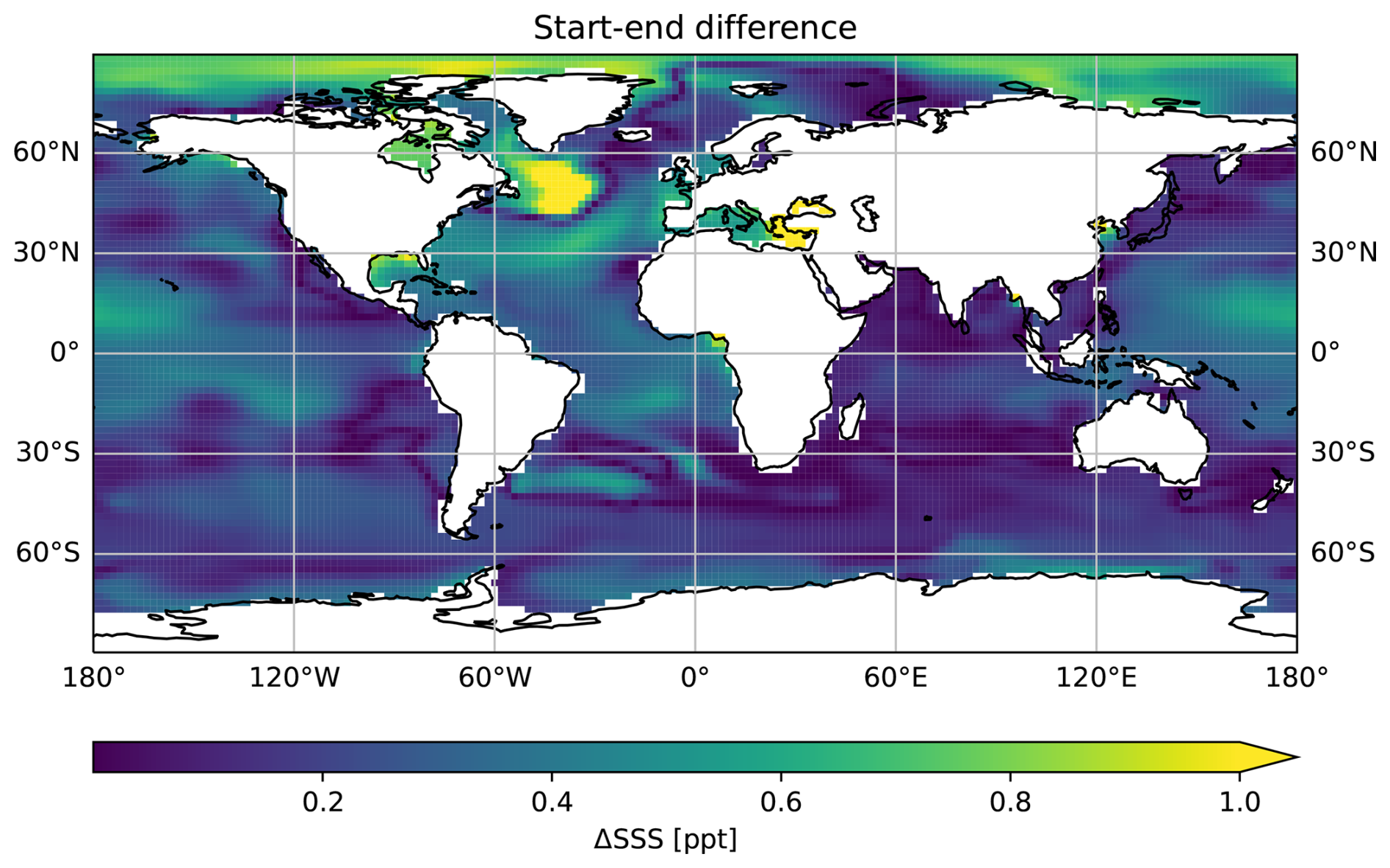
Figure A1Difference between the start (year 1850) and end (year 2100) of the dataset (GISS-E2-1-G, SSP245, ensemble r1i1p5f1) for SSS, measured in parts per thousand (ppt). Since we use the 10-year running mean, we use years 1855 and 2095 as the first and last year, respectively. In the region finding approach, we select regions that have a high start-end difference compared to the rest of the dataset, such as for example the polar-latitudes and the subpolar-gyre. The result of the region-selection is illustrated in Fig. A2.
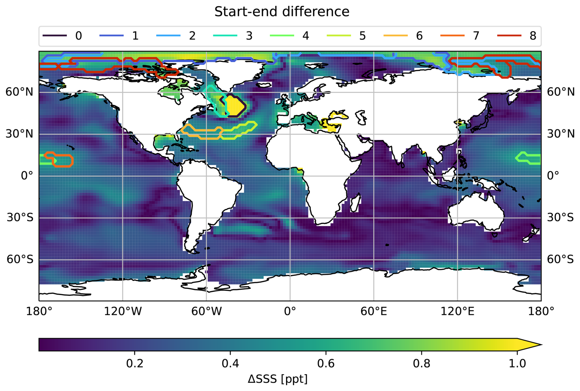
Figure A2Difference between the start and end of the dataset (GISS-E2-1-G, SSP245, ensemble r1i1p5f1) for SSS, like Fig. A1, with the nine identified regions (labelled from 0–8) overlaid. The order of the regions is determined by the order in which the regions are selected. This means that region 0, the sub-polar gyre, was first identified as it was the first region to surpass (high) a percentile threshold and be of ≥106 km2.
Table A1The CMIP6 variables along with their short notation (used throughout this paper) as well as the CMIP6 description. The variables msftyz and msftmz have a different data-format than the other CMIP6 variables, which are surface variables. The handling of msftyz and msftmz is therefore different as discussed in Sect. 2 and only criterion St2 is applied to this data.
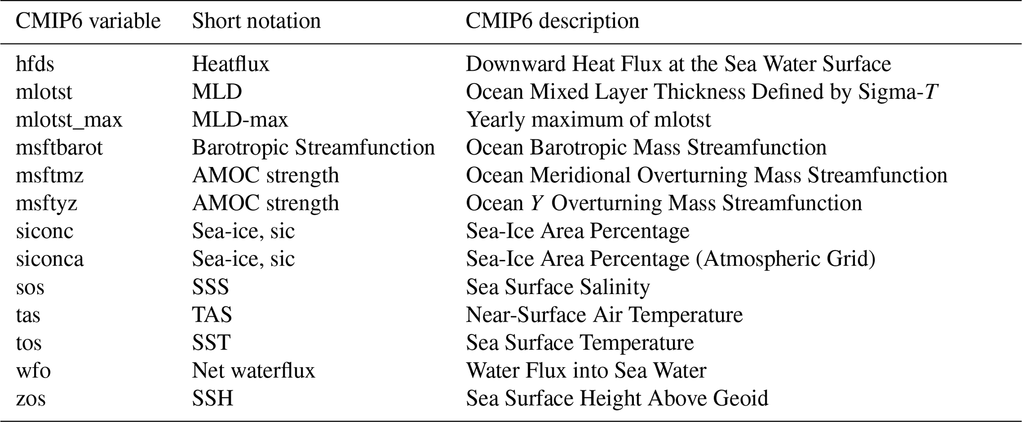
The difference between the start and end of the time series (years 1855 and 2095 respectively, because of the 10-year running mean) is illustrated in Fig. A1. We now describe step by step how the start-end difference region isolation approach (Sect. 2.2) selects regions from this 2D-map. The method first evaluates if any region passes a very high threshold of the 99.99 %-percentile. For didactic purposes, let's assume this threshold corresponds to 1.0 parts per thousand (ppt). We produce a Boolean map if the start-end difference exceeds this threshold. Using an unsupervised clustering algorithm (Campello et al., 2013), we build continuous regions of the Boolean map. This yields one or more clusters on the map with regions higher than the 1.0 ppt criterion. Now, we only keep those clusters that also exceed the area-requirement of 106 km2. It happens rarely that the first threshold (99.99 %) yields any regions that are sufficiently large (since only 0.01 % of the grid-cells should exceed it). So let us assume we did not find any cluster at the first iteration. If we lower the threshold, and run the algorithm again (for example, with a threshold of 0.9 ppt difference), the clusters are generally larger than in previous step. It may now happen that a clustered region is sufficiently large. We save this region, but also check again if a lower threshold (for example, 0.8 ppt) yields any new clusters. We emphasize that it should be new, since we exclude the first selected cluster from the Boolean mask (since we already identified that region). We keep repeating these steps, so at the lowest percentile (85 %), we have most likely already identified some regions, usually in the order of 1–10 regions. These 1–10 regions are then the input for the next phase (Sect. 2.3). To illustrate the contrast to the explained method, we could have instead only applied the 85 %-percentile threshold. We would have gotten for example, two regions that ∼ 5–10 × 106 km2. These two regions might then wash out any SNS, which is not in line with the goal of this step. This is why we iterate the thresholds to get smaller regions (≥106 km2) such that we obtain sufficiently fine-grained regions to identify SNS.
The iterative approach described above, applied to Fig. A1, will first select the large start-end difference near the subpolar gyre, followed by regions near the arctic. When the actual thresholds of the method are used, this method isolates nine distinct regions to be passed on to the next step, where we check each region for the occurrence of SNS. The nine distinct regions are illustrated in Fig. A2.
The other three approaches (see Sect. 2.2) to identify regions work similarly and are all available online https://github.com/JoranAngevaare/optim_esm_tools/blob/master/notebooks/advanced_methods.ipynb (last access: 17 July 2026) (Angevaare, 2025a). Furthermore, this material also illustrates how the regions from multiple approaches are joined in the next step of the algorithm where the formal criteria are applied and regions are iteratively expanded (Sect. 2.3).
A2 Formal criteria
Below we give the six criteria and their respective thresholds. The criteria were designed to isolate regions with spatially averaged time series that are extreme for the available CMIP6 data. Criteria Ab1 and Ab2 are specifically designed to select regimes that feature a single abrupt change. These two criteria are general purpose and are applied to all CMIP6 variables in Table A1. Criteria St1-St4 are instead formalized to select large-scale state transitions, which occur on longer timescales. Criteria St1-St3 are for specific variables, while criterion St4 is general purpose.
The criteria use slightly different metrics to achieve these aims. Below, we discuss the criteria one by one. Most metrics are related, e.g. the abrupt criteria (Ab1 and Ab2) use a maximum jump in 10 years in the time series in places where the state transition (criterion St4) uses the difference between the start and end of the time series. The selection of each threshold in the criteria below was an iterative process and based on careful selection by the authors. They are therefore subjective, and while criteria Ab1, Ab2 and St4 are designed to be general purpose, CMIP6 variables that were not investigated in this work may require better suited thresholds or optimized criteria.
A2.1 Criterion Ab1
Criterion Ab1 is designed to select abrupt changes. To this end we calculate the spatially averaged time series (below, we will simply call this the time series) of an isolated variable (Fig. 1). As we are interested in large changes in the time series, we calculate the maximum jump (MJ) in a 10-year window, after smoothing the time series with a 10-year running mean. We want the maximum jump to be large with respect to the pi-control dataset and the average variability in the scenario dataset. To this end, we calculate the standard deviation of the 10-year running mean of the detrended time series of the pi-control dataset within the region, which we call σPiC. We require that the jump seen in the scenario is at least 4.5×σPiC as in the first line of Eq. (A1).
Additionally, we calculate the average standard deviation of all cells, based on their individual 10-year running mean of the detrended values. This gives us a measure of the average global variability in the pi-control. However, since the tropical latitudes have different average standard deviations, we only take the average over grid cells within the 23.5° S:23.5° N band if 50 % of the grid cells of the selected region are in that latitude range. In case the selected region has less than 50 % in the 23.5° S:23.5° N-band, we instead take the average over grid cells that are outside this band. We call this average standard-deviation of the pi-control dataset . We require that MJ is extreme, compared to the average variability in that zone (either tropics or outside of the tropics) by imposing (second line of Eq. A1).
Similar to , we also require that the MJ is extreme with respect to the average standard-deviation of the 10-year running mean of the detrended time series in a large-scale zone (tropics or outside tropics). Completely analogous to , we call this average require that it is 5× smaller than MJ.
Furthermore, we require that the (un-smoothed, yearly) time series is not unimodal, but bi- or multimodal by applying the dip test for unimodality (Hartigan and Hartigan, 1985) and requiring that its value is below 1 %.
Finally, we select time series that show one clearly identifiable jump. We compare the largest jump (MJ) to the second largest jump of the same sign (that is at least 10 years removed from MJ). We call the ratio between these two jumps J2. As some time series have both increasing and decreasing jumps, we also explicitly calculate the largest jump that has the opposite sign from the largest jump anywhere in the time series. The ratio between these jumps we similarly call J2min.
Together, the thresholds in Equation A1 select time series with single, abrupt (in the timescale of 10-year) jumps in the time series that are unique for this region, as well as large when compared to the standard deviation of either averages of the pi-control or scenario datasets. The abruptness should cause a detectable bi/multi-modality to pass the Diptest. The full criterion reads:
A2.2 Criterion Ab2
Criterion Ab2, similar to criterion Ab1, aims to detect abrupt changes. Criterion Ab1 often fails to identify abrupt changes when they occur at the end (or, theoretically, start) of the time series. When this occurs, a second state is not sufficiently sampled to pass the Diptest. By dropping the Diptest and increasing the requirement on the J2 and J2min parameters, we are able to select this type of time series that fail criterion Ab1. This leads to:
A2.3 Criterion St1
Criterion St1 aims to select (almost) complete disappearance of sea-ice in a large-scale area. For an arbitrary region, this could easily be achieved, as a peripheral region of sea-ice may melt in a warming climate (e.g. starting from 50 % sea-ice cover and ending with 0 %). Therefore, we require the regions to be at least 5×10⁶ km2. Additionally, we require that the disappearance is at least 95 % of the maximal value in an area that is at least as large. We compute the maximal average in a connected area (if it is of the same size) with the maximal sea-ice values. The ratio between the start and end time of the region of interest and this maximum value is what we call ES, which should exceed 95 %:
A2.4 Criterion St2
Criterion St2 is similar to criterion St1 and focuses on a large percentage drop in the time series. This criterion applies only to msftyz, msftmz, and it uses the workflow as described in (Drijfhout et al., 2025) to analyze this data format. We calculate the decline between the maximum in the 10-year running mean (max(vrm 10(t))) and the last value in the 10-year running mean (vrm 10(t=tend)), which we call . We require that there is a loss of at least 70 % of the maximal value, as in the equation below:
A2.5 Criterion St3
Criterion St3 is meant to isolate regions of dramatic and persistent loss of mixed-layer depth. We utilize a longer running mean of 50 years since the mixed-layer depth often shows large inter-annual variability. We require, analogous to criterion St2, that the change of the 50-year running mean of the time series since the maximum is 90 % of that maximum. Additionally, we use σPiC rm 50 to filter out regions that also have large variability in the pi-control dataset (similar to criteria Ab1 and Ab2). Finally, we also use MEtrop rm 50, which is the difference between the maximum and end of the spatially averaged time series in the tropics/outside the tropics. With this last metric, we also filter out regions that are showing large declines when considering only that region but are not standing out significantly when considering a large zonal average. Combining these metrics leads to:
A2.6 Criterion St4
Criterion St4 is applied to variables not yet covered by criteria St1-St3. As a general-purpose search for state transitions, it uses the difference between start and end of the time series (SE), which has to be extreme compared to certain metrics. We compare SE to σPiC trop and σPiC which have been discussed above. Similar to (criterion St3), we also here formulate a requirement on (although in contrast to mlotst-max, this value may be negative, so an absolute value is required). Finally, we filter out time series with a large decadal variability. We use the standard-deviation of the difference in the 50 and 10 year running mean (SD(vrm 50(t)−vrm 10(t))) and require that SE is large with respect to this number. Combined, this leads to the following requirement:
A3 Variables and available data
We used CMIP6 variables in this work which we list, together with their short notations, in Table A1.
In Table A2 we list all the available data used for making this catalogue. The data are limited to those available at the time of writing, sets where a matching pi-control, historical and scenario run is complete and available.
Table A2Number of ensemble-members per model, per variable, per SSP. For each variable we list the five SSPs separated by commas such that e.g. “hfds: 0, 0, 1, 2, 1” indicates 0 × SSP119, 0 × SSP126, 1 × SSP245, 2 × SSP370, 1 × SSP585 for hfds.
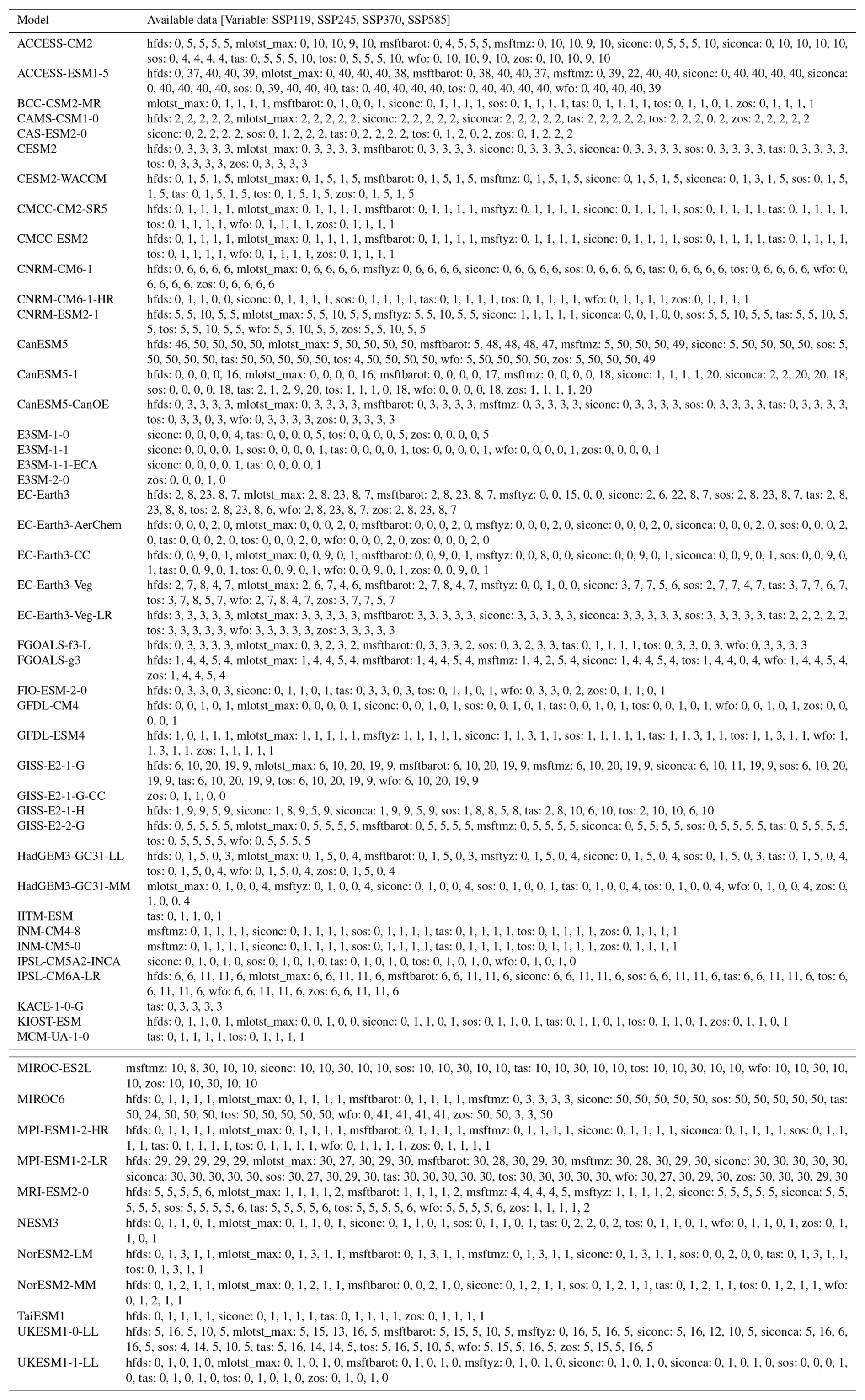
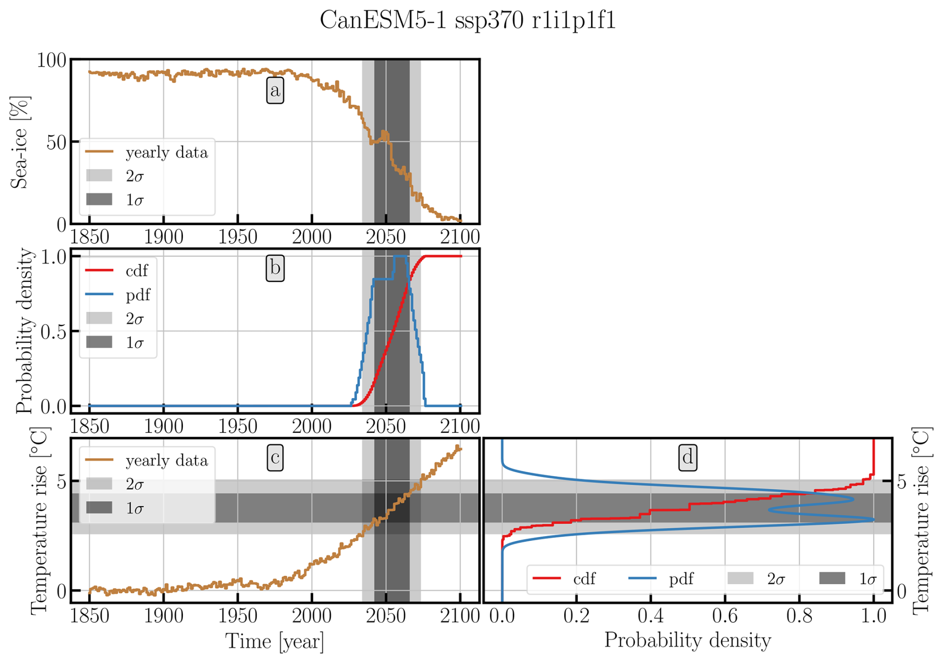
Figure A3Method of obtaining the global temperature rise at shift for an SNS. We analyze the yearly data of panel (a) (see text for details) to determine when the change is maximal. The resulting CDF and PDF are shown in panel (b). Based on the CDF in panel (b), we draw the vertical 1σ and 2σ probability intervals. In panel (c), we add the global temperature rise relative to the 1850–1880 average. By weighing the temperature rise values with the PDF of panel (b) we can calculate panel (d), where we show the CDF and the PDF of the shift to occur at a certain temperature rise. The PDF in panel (d) is smoothed by a Gaussian with a standard deviation of 0.2 °C for illustration purposes. The horizontal 1σ and 2σ probability intervals are based on the CDF of panel (d).
A4 Temperature at maximal change of an SNS
In Sect. 4 and Fig. 17 we discuss the PDF/CDF (Cumulative Distribution Function) of shifts occurring at a certain global temperature rise. Fig. A3 illustrates the method for obtaining the PDF/CDF for an example time series (SNS #6 of Table A3). To do this, we analyze the spatially averaged time series of an SNS, as shown in panel a. First, we determine the time at which the change occurs. We find the largest change in a w-year window in the time series that we smooth by a w-year running mean. We assign an equal probability to all years within that w-year window. We repeat this for w from 20 to 50 years, as SNS typically evolve on such timescales. This results in the PDF and CDF in panel b of Fig. A3.
To account for this, we take all temperatures in a window (w) into account around the year where the w-year difference in the time series is maximal (a w-year running mean). Each temperature within that time region is treated with equal probability. We repeat this for w from 20 to 50 year to build a temperature distribution at which the change is maximal. Panel b shows the PDF and CDF of the timing at which the change is maximal. By weighing the temperature change since 1850–1880 (panel c) with the PDF from panel b, we are able to build a PDF of the shift occurring at a certain temperature rise (panel d).
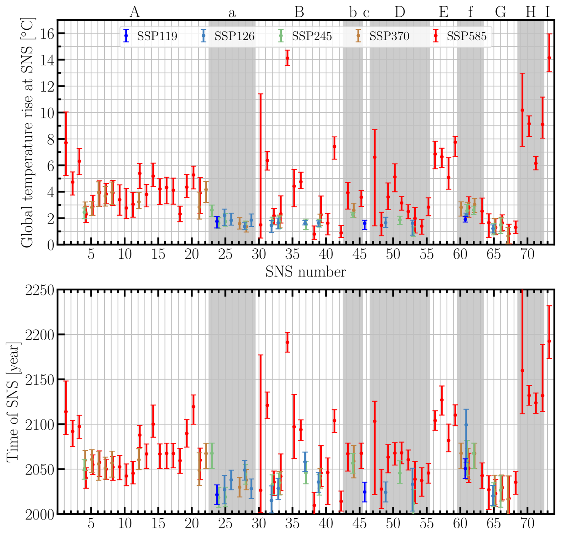
Figure A4Median global temperature rise at SNS for all 73 SNS. The error bars indicate the 1σ confidence interval. Per case, the contributions of the SSPs are split (and slightly shifted horizontally for illustration purposes). The letters (top) denote the category to which the SNS belong and the categories are also illustrated using alternating background shades.
A5 SNS
In Table A3 we include each of the 73 SNS. As apparent from the table, one SNS is the occurrence of an event of one of the 11 SNS categories in a model. One SNS can be manifested in multiple variables or SSPs, as long as their associated regions are spatially overlapping. Some categories span a large spatial region, for this reason one model can result in more than one SNS per category, for example #8 and #9 in Table A3.
The global temperature rise at the time of the SNS within a given category may vary significantly per model (as we have seen in Fig. 15). We can instead also calculate the CDF per SNS, as shown in Fig. A4. Each of the 73 cases is plotted separately, and split per SSP. As expected from Fig. A3, the 1σ-confidence interval in Fig. A4 can be skewed, depending on the evolution of the time series and global temperature rise within the model.
Figure A5 illustrates the first ensemble-member per case, where we show each variable per SNS category in a single panel.
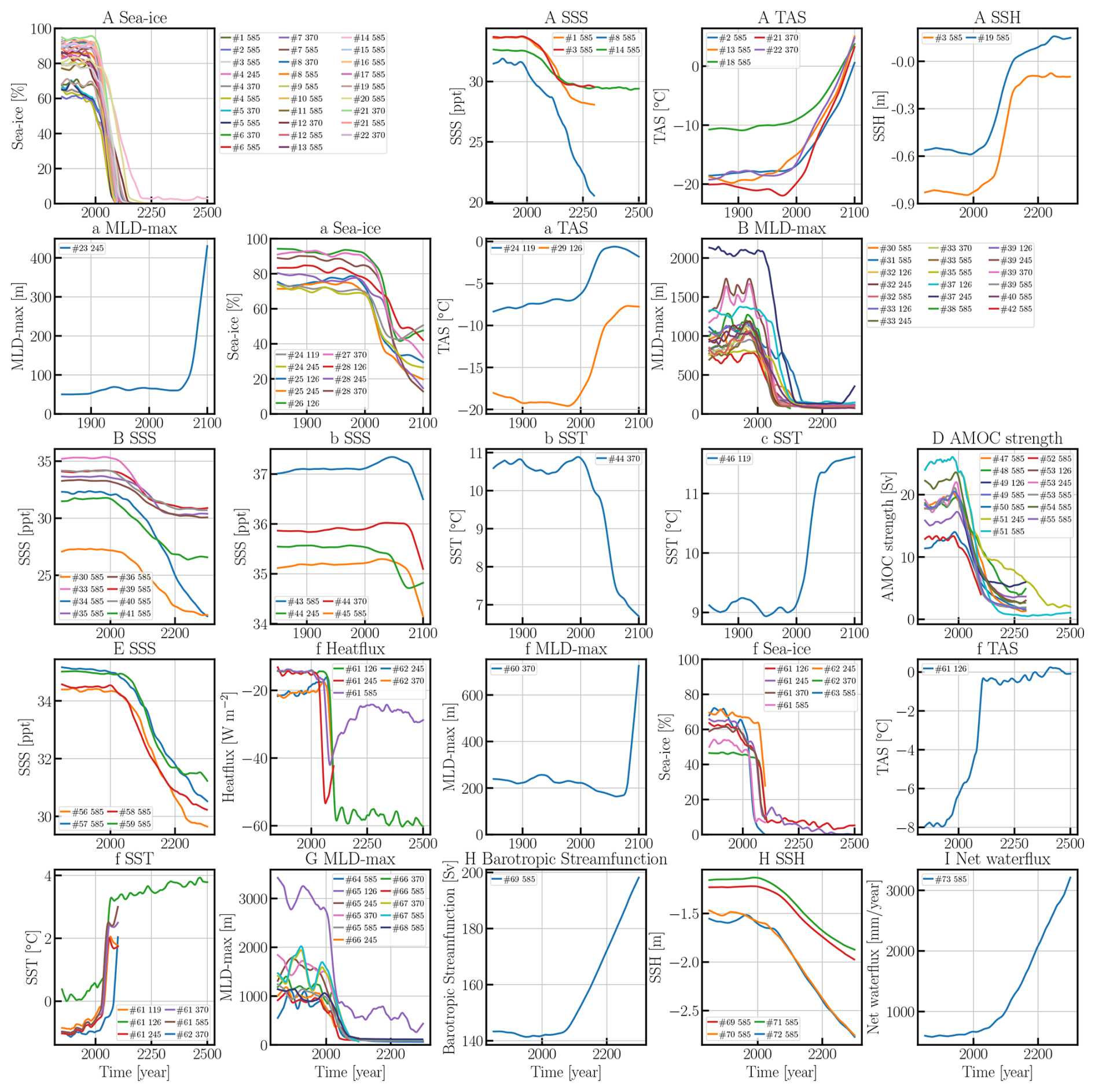
Figure A5Time series of the first ensemble-member of each SNS case from Table A3. The time series are split per SNS category, and per variable within the SNS category, represented by the title of each panel. The legend labels refer to the SNS number in Table A3 and the SSP (119, 126, 245, 370 or 585). For illustration purposes, the time series are smoothed using a Lowess filter with a window of 40 years. Also see (Angevaare and Drijfhout, 2025b) for each case separately.
Table A3List of all 73 SNS and attributes of each SNS. The associated SNS category (cat.) and SSP(s) are listed. The criteria (crit.) and variables (Vars) that are found at least once for each case and associated region are also listed. See text for more information. Also see Angevaare and Drijfhout (2025b) for each case separately.
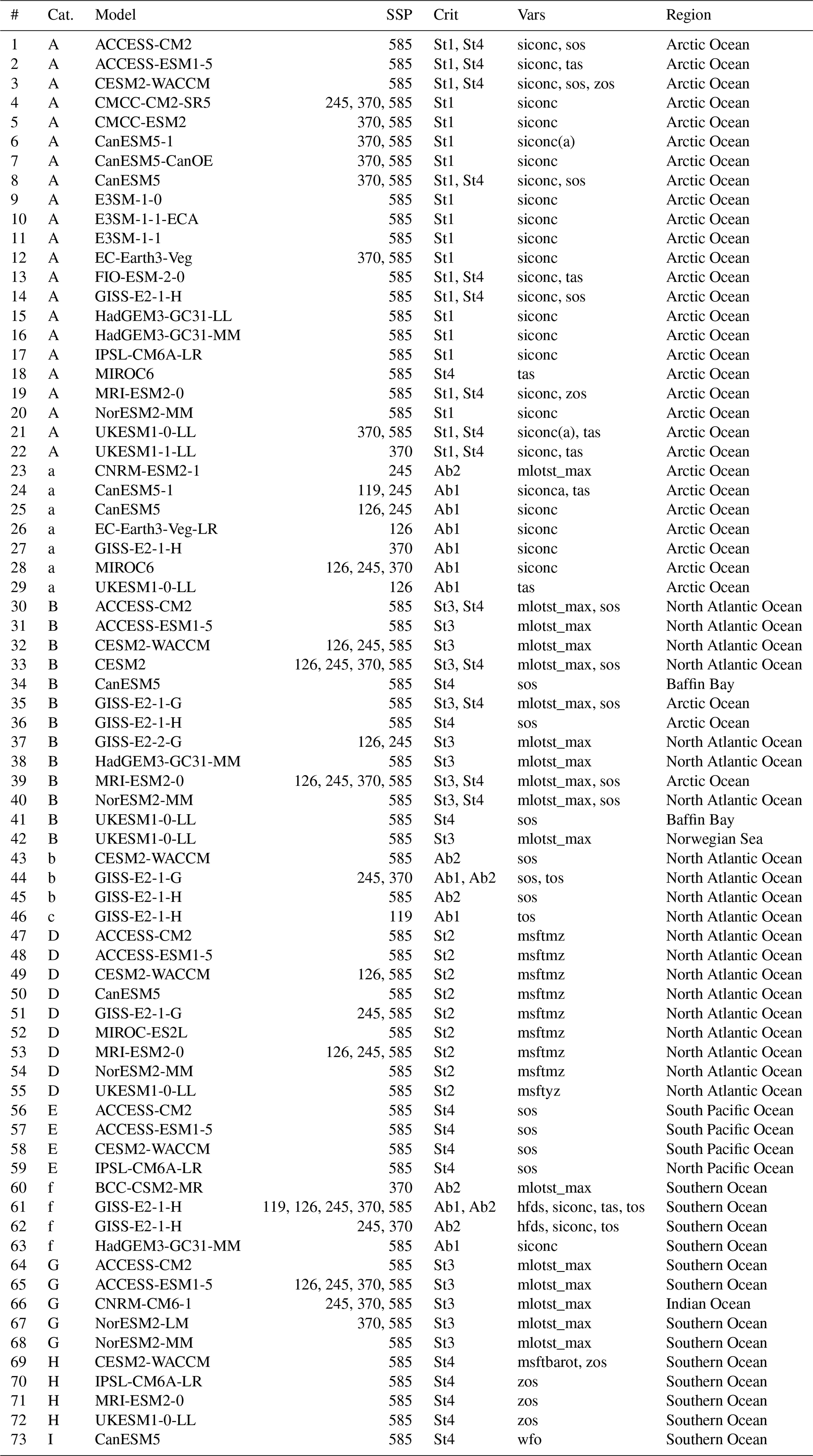
The framework (Angevaare, 2025a) for this work is available at https://github.com/JoranAngevaare/optim_esm_tools (last access: 17 July 2026; DOI: https://doi.org/10.5281/zenodo.15275185).
The CMIP6 data used in this work is freely available online at https://esgf-node.llnl.gov/search/cmip6/ (last access: 17 July 2026). The identified SNS cases from this work are available at https://doi.org/10.5281/zenodo.17867115 (Angevaare and Drijfhout, 2025b).
JRA and SSD designed the study, JRA implemented the study, JRA produced the figures, JRA and SSD wrote and edited the paper.
The contact author has declared that neither of the authors has any competing interests.
Publisher's note: Copernicus Publications remains neutral with regard to jurisdictional claims made in the text, published maps, institutional affiliations, or any other geographical representation in this paper. The authors bear the ultimate responsibility for providing appropriate place names. Views expressed in the text are those of the authors and do not necessarily reflect the views of the publisher.
We acknowledge the World Climate Research Programs Working Group on Coupled Modeling, which is responsible for CMIP, and we thank the climate modelling groups (listed in Table A2 of this paper) for producing and making available their model output. For CMIP the U.S. Department of Energy's Program for Climate Model Diagnosis and Intercomparison provides coordinating support and led development of software infrastructure in partnership with the Global Organization for Earth System Science Portals. We thank the climate modelling groups for producing and making available their model output, the Earth System Grid Federation (ESGF) for archiving the data and providing access, and the multiple funding agencies who support CMIP6 and ESGF. The CMIP6 data was accessed and analysed using the Netherlands super-computer-cluster SURFsara.
SSD and JRA received funding from OptimESM and SSD from TipESM. TipESM “Exploring Tipping Points and Their Impacts Using Earth System Models” is funded by the European Union. Grant Agreement number: 101137673. OptimESM, “Optimal High Resolution Earth System Models for Exploring Future Climate Change” is funded by the European Union. Grant Agreement number: 101081193. SSD received funding from ISOTIPIC. ISOTIPIC, “Interacting ice Sheet and Ocean Tipping – Indicators, Processes, Impacts and Challenges” is funded by the National Environmental Research Council, UK, under Grant Number: NE/Y503320/1.
This research has been supported by the HORIZON EUROPE Climate, Energy and Mobility (grant nos. 101081193 and 101137673) and the Natural Environment Research Council (grant no. NE/Y503320/1).
This paper was edited by Jonathan Donges and reviewed by four anonymous referees.
Abbot, D. S., Huber, M., Bousquet, G., and Walker, C. C.: High-CO2 cloud radiative forcing feedback over both land and ocean in a global climate model, Geophys. Res. Lett., 36, https://doi.org/10.1029/2008GL036703, 2009. a
Angevaare, J. R.: JoranAngevaare/optim_esm_tools: v4.0.0, Zenodo [code], https://doi.org/10.5281/zenodo.15275185, 2025a. a, b, c, d
Angevaare, J. R. and Drijfhout, S. S.: JoranAngevaare/Catalogue-of-Strong-Nonlinear- Surprises-in-ocean-sea-ice-and-atmospheric- variables-in-CMIP6, Zenodo [data set], https://doi.org/10.5281/zenodo.17867115, 2025b. a, b, c, d, e
Armstrong McKay, D. I., Staal, A., Abrams, J. F., Winkelmann, R., Sakschewski, B., Loriani, S., Fetzer, I., Cornell, S. E., Rockström, J., and Lenton, T. M.: Exceeding 1.5 C global warming could trigger multiple climate tipping points, Science, 377, eabn7950, https://doi.org/10.1126/science.abn7950, 2022. a, b, c, d, e, f, g, h, i
Bathiany, S., Hidding, J., and Scheffer, M.: Edge detection reveals abrupt and extreme climate events, J. Climate, 33, 6399–6421, https://doi.org/10.1175/JCLI-D-19-0449.1, 2020. a
Boers, N.: Observation-based early-warning signals for a collapse of the Atlantic Meridional Overturning Circulation, Nat. Clim. Change, 11, 680–688, https://doi.org/10.1038/s41558-021-01097-4, 2021. a
Bracegirdle, T. J., Shuckburgh, E., Sallee, J.-B., Wang, Z., Meijers, A. J., Bruneau, N., Phillips, T., and Wilcox, L. J.: Assessment of surface winds over the Atlantic, Indian, and Pacific Ocean sectors of the Southern Ocean in CMIP5 models: Historical bias, forcing response, and state dependence, J. Geophys. Res.-Atmos., 118, 547–562, https://doi.org/10.1002/jgrd.50153, 2013. a, b
Campello, R. J. G. B., Moulavi, D., and Sander, J.: Density-Based Clustering Based on Hierarchical Density Estimates, in: Advances in Knowledge Discovery and Data Mining, edited by: Pei, J., Tseng, V. S., Cao, L., Motoda, H., and Xu, G., 160–172, Springer Berlin Heidelberg, Berlin, Heidelberg, ISBN 978-3-642-37456-2, https://doi.org/10.1007/978-3-642-37456-2_14, 2013. a, b
Canny, J.: A computational approach to edge detection, IEEE T. Pattern Anal., 6, 679–698, https://doi.org/10.1109/TPAMI.1986.4767851, 1986. a
Davy, R. and Griewank, P.: Arctic amplification has already peaked, Environ. Res. Lett., 18, 084003, https://doi.org/10.1088/1748-9326/ace273, 2023. a
De Lavergne, C., Palter, J. B., Galbraith, E. D., Bernardello, R., and Marinov, I.: Cessation of deep convection in the open Southern Ocean under anthropogenic climate change, Nat. Clim. Change, 4, 278–282, https://doi.org/10.1038/nclimate2132, 2014. a
Ditlevsen, P. and Ditlevsen, S.: Warning of a forthcoming collapse of the Atlantic meridional overturning circulation, Nat. Commun., 14, 1–12, https://doi.org/10.1038/s41467-023-39810-w, 2023. a
Drews, A., Greatbatch, R. J., Ding, H., Latif, M., and Park, W.: The use of a flow field correction technique for alleviating the North Atlantic cold bias with application to the Kiel Climate Model, Ocean Dynam., 65, 1079–1093, https://doi.org/10.1007/s10236-015-0853-7, 2015. a
Drijfhout, S., Bathiany, S., Beaulieu, C., Brovkin, V., Claussen, M., Huntingford, C., Scheffer, M., Sgubin, G., and Swingedouw, D.: Catalogue of abrupt shifts in Intergovernmental Panel on Climate Change climate models, P. Natl. Acad. Sci. USA, 112, E5777–E5786, https://doi.org/10.1073/pnas.1511451112, 2015. a, b, c, d, e, f, g, h, i, j, k, l, m, n, o, p, q, r, s, t, u, v, w, x, y
Drijfhout, S., Angevaare, J. R., Mecking, J., van Westen, R. M., and Rahmstorf, S.: Shutdown of northern Atlantic overturning after 2100 following deep mixing collapse in CMIP6 projections, Environ. Res. Lett., 20, 094062, https://doi.org/10.1088/1748-9326/adfa3b, 2025. a, b, c, d, e, f, g, h, i, j, k, l, m
Drijfhout, S. S., Bull, C. Y., Hewitt, H., Holland, P. R., Jenkins, A., Mathiot, P., and Garabato, A. N.: An Amundsen Sea source of decadal temperature changes on the Antarctic continental shelf, Ocean Dynam., 74, 37–52, https://doi.org/10.1007/s10236-023-01587-3, 2024. a
Feldl, N., Po-Chedley, S., Singh, H. K., Hay, S., and Kushner, P. J.: Sea ice and atmospheric circulation shape the high-latitude lapse rate feedback, NPJ Climate and Atmospheric Science, 3, 41, https://doi.org/10.1038/s41612-020-00146-7, 2020. a
Fox-Kemper, B., Hewitt, H. T., Xiao, C., Adalgeirsdóttir, G., Drijfhout, S. S., Edwards, T. L., Golledge, N. R., Hemer, M., Kopp, R. E., Krinner, G., Mix, A., Notz, D., Nowicki, S., Nurhati, I., Ruiz, L., Sallée, J.-B., Slangen, A., and Yu, Y.: Ocean, cryosphere, and sea level change, in: Climate Change 2021: The Physical Science Basis. Contribution of Working Group I to the Sixth Assessment Report of the Intergovernmental Panel on Climate Change, Cambridge University Press, 1211–1361, https://doi.org/10.1017/9781009157896.011, 2021. a, b
Geen, R., Bordoni, S., Battisti, D. S., and Hui, K.: Monsoons, ITCZs, and the Concept of the Global Monsoon, Rev. Geophys., 58, e2020RG000700, https://doi.org/10.1029/2020RG000700, 2020. a
Gómez-Valdivia, F., Holland, P. R., Siahaan, A., Dutrieux, P., and Young, E.: Projected West Antarctic ocean warming caused by an expansion of the Ross Gyre, Geophys. Res. Lett., 50, e2023GL102978, https://doi.org/10.1029/2023GL102978, 2023. a
Hankel, C. and Tziperman, E.: The role of atmospheric feedbacks in abrupt winter Arctic sea ice loss in future warming scenarios, J. Climate, 34, 4435–4447, https://doi.org/10.1175/JCLI-D-20-0558.1, 2021. a
Hankel, C. and Tziperman, E.: Assessing the Robustness of Arctic Sea Ice Bi-Stability in the Presence of Atmospheric Feedbacks, J. Geophys. Res.-Atmos., 128, e2023JD039337, https://doi.org/10.1029/2023JD039337, 2023. a
Hartigan, J. A. and Hartigan, P. M.: The dip test of unimodality, Ann. Stat., 13, 70–84, https://doi.org/10.1214/aos/1176346577, 1985. a, b
Heuzé, C.: Antarctic Bottom Water and North Atlantic Deep Water in CMIP6 models, Ocean Sci., 17, 59–90, https://doi.org/10.5194/os-17-59-2021, 2021. a
Holland, P. R., Bracegirdle, T. J., Dutrieux, P., Jenkins, A., and Steig, E. J.: West Antarctic ice loss influenced by internal climate variability and anthropogenic forcing, Nat. Geosci., 12, 718–724, https://doi.org/10.1038/s41561-019-0420-9, 2019. a, b, c
Hwang, Y.-T. and Frierson, D. M.: Link between the double-Intertropical Convergence Zone problem and cloud biases over the Southern Ocean, P. Natl. Acad. Sci. USA, 110, 4935–4940, https://doi.org/10.1073/pnas.1213302110, 2013. a
Jesse, F., Le Bars, D., and Drijfhout, S.: Processes explaining increased ocean dynamic sea level in the North Sea in CMIP6, Environ. Res. Lett., 19, 044060, https://doi.org/10.1088/1748-9326/ad33d4, 2024. a
Kay, J. E., Holland, M. M., Bitz, C. M., Blanchard-Wrigglesworth, E., Gettelman, A., Conley, A., and Bailey, D.: The influence of local feedbacks and northward heat transport on the equilibrium Arctic climate response to increased greenhouse gas forcing, J. Climate, 25, 5433–5450, https://doi.org/10.1175/JCLI-D-11-00622.1, 2012. a
Kopp, R. E., Gilmore, E. A., Shwom, R. L., Adams, H., Adler, C., Oppenheimer, M., Patwardhan, A., Russill, C., Schmidt, D. N., and York, R.: `Tipping points' confuse and can distract from urgent climate action, Nat. Clim. Change, 15, 29–36, https://doi.org/10.1038/s41558-024-02196-8, 2025. a, b
Kuhlbrodt, T., Titz, S., Feudel, U., and Rahmstorf, S.: A simple model of seasonal open ocean convection: Part II: Labrador Sea stability and stochastic forcing, Ocean Dynam., 52, 36–49, https://doi.org/10.1007/s10236-001-8175-3, 2001. a
Lee, J.-Y., Marotzke, J., Bala, G., Cao, L., Corti, S., Dunne, J., Engelbrecht, F., Fischer, E., Fyfe, J., Jones, C., Maycock, A., Mutemi, J., Niaye, O., Panickal, S., Zhou, T., and Christensen, H.: Future global climate: scenario-based projections and near-term information, IPCC Assessment Reports, Cambridge University Press, 553–672, https://doi.org/10.1017/9781009157896.006, 2021. a
Lenderink, G. and Haarsma, R. J.: Modeling Convective Transitions in the Presence of Sea lce, J. Phys. Oceanogr., 26, 1448–1467, https://doi.org/10.1175/1520-0485(1996)026<1448:MCTITP>2.0.CO;2, 1996. a
Lenton, T. M., Held, H., Kriegler, E., Hall, J. W., Lucht, W., Rahmstorf, S., and Schellnhuber, H. J.: Tipping elements in the Earth's climate system, P. Natl. Acad. Sci. USA, 105, 1786–1793, https://doi.org/10.1073/pnas.0705414105, 2008. a
Loriani, S., Aksenov, Y., Armstrong McKay, D. I., Bala, G., Born, A., Chiessi, C. M., Dijkstra, H. A., Donges, J. F., Drijfhout, S., England, M. H., Fedorov, A. V., Jackson, L. C., Kornhuber, K., Messori, G., Pausata, F. S. R., Rynders, S., Sallée, J.-B., Sinha, B., Sherwood, S. C., Swingedouw, D., and Tharammal, T.: Tipping points in ocean and atmosphere circulations, Earth Syst. Dynam., 16, 1611–1653, https://doi.org/10.5194/esd-16-1611-2025, 2025. a, b, c, d
Mchedlishvili, A., Spreen, G., Melsheimer, C., and Huntemann, M.: Weddell Sea polynya analysis using SMOS–SMAP apparent sea ice thickness retrieval, The Cryosphere, 16, 471–487, https://doi.org/10.5194/tc-16-471-2022, 2022. a, b
McInnes, L. and Healy, J.: Accelerated hierarchical density based clustering, in: 2017 IEEE international conference on data mining workshops (ICDMW), IEEE, 33–42, https://doi.org/10.1109/ICDMW.2017.12, 2017. a
Mecking, J. V. and Drijfhout, S. S.: The decrease in ocean heat transport in response to global warming, Nat. Clim. Change, 13, 1229–1236, https://doi.org/10.1038/s41558-023-01829-8, 2023. a, b
Menary, M. B., Robson, J., Allan, R. P., Booth, B. B. B., Cassou, C., Gastineau, G., Gregory, J., Hodson, D., Jones, C., Mignot, J., Ringer, M., Sutton, R., Wilcox, L., and Zhang, R.: Aerosol-Forced AMOC Changes in CMIP6 Historical Simulations, Geophys. Res. Lett., 47, e2020GL088166, https://doi.org/10.1029/2020GL088166, e2020GL088166 2020GL088166, 2020. a
Meredith, M., Sommerkorn, M., Cassotta, S., Derksen, C., Ekaykin, A., Hollowed, A., Kofinas, G., Mackintosh, A., Muelbert, M., Melbourne-Thomas, J., Ottersen, G., Pritchard, H., and Schuur, E.: Chapter 3: Polar Regions, in: The Ocean and Cryosphere in a Changing Climate, edited by: Anisimov, O., Flato, G., and Xiao, C., Intergovernmental Panel on Climate Change, 3-1–3-173, https://doi.org/10.1017/9781009157964.005, 2019. a
Moreno-Chamarro, E., Caron, L.-P., Loosveldt Tomas, S., Vegas-Regidor, J., Gutjahr, O., Moine, M.-P., Putrasahan, D., Roberts, C. D., Roberts, M. J., Senan, R., Terray, L., Tourigny, E., and Vidale, P. L.: Impact of increased resolution on long-standing biases in HighResMIP-PRIMAVERA climate models, Geosci. Model Dev., 15, 269–289, https://doi.org/10.5194/gmd-15-269-2022, 2022. a, b
Morioka, Y., Manabe, S., Zhang, L., Delworth, T. L., Cooke, W., Nonaka, M., and Behera, S. K.: Antarctic sea ice multidecadal variability triggered by Southern Annular Mode and deep convection, Communications Earth & Environment, 5, 633, https://doi.org/10.1038/s43247-024-01783-z, 2024. a
Munday, D. R., Johnson, H. L., and Marshall, D. P.: Eddy saturation of equilibrated circumpolar currents, J. Phys. Oceanogr., 43, 507–532, https://doi.org/10.1175/JPO-D-12-095.1, 2013. a
Naughten, K. A., Holland, P. R., Dutrieux, P., Kimura, S., Bett, D. T., and Jenkins, A.: Simulated twentieth-century ocean warming in the Amundsen Sea, West Antarctica, Geophys. Res. Lett., 49, e2021GL094566, https://doi.org/10.1029/2021GL094566, 2022. a, b
Notz, D. and SIMIP Community: Arctic Sea Ice in CMIP6, Geophys. Res. Lett., 47, e2019GL086749, https://doi.org/10.1029/2019GL086749, 2020. a
O'Neill, B. C., Tebaldi, C., van Vuuren, D. P., Eyring, V., Friedlingstein, P., Hurtt, G., Knutti, R., Kriegler, E., Lamarque, J.-F., Lowe, J., Meehl, G. A., Moss, R., Riahi, K., and Sanderson, B. M.: The Scenario Model Intercomparison Project (ScenarioMIP) for CMIP6, Geosci. Model Dev., 9, 3461–3482, https://doi.org/10.5194/gmd-9-3461-2016, 2016. a
Portmann, V., Swingedouw, D., Khattab, O., and Chavent, M.: Observational constraints project a ∼ 50 % AMOC weakening by the end of this century, Science Advances, 12, eadx4298, https://doi.org/10.1126/sciadv.adx4298, 2026. a, b
Rheinlænder, J. W., Smedsrud, L. H., and Nisanciouglu, K. H.: Internal ocean dynamics control the long-term evolution of Weddell Sea Polynya activity, Frontiers in Climate, 3, 718016, https://doi.org/10.3389/fclim.2021.718016, 2021. a, b
Robson, J., Menary, M. B., Sutton, R. T., Mecking, J., Gregory, J. M., Jones, C., Sinha, B., Stevens, D. P., and Wilcox, L. J.: The Role of Anthropogenic Aerosol Forcing in the 1850–1985 Strengthening of the AMOC in CMIP6 Historical Simulations, J. Climate, 35, 6843–6863, https://doi.org/10.1175/JCLI-D-22-0124.1, 2022. a
Romanou, A., Rind, D., Jonas, J., Miller, R., Kelley, M., Russell, G., Orbe, C., Nazarenko, L., Latto, R., and Schmidt, G. A.: Stochastic Bifurcation of the North Atlantic Circulation under a Midrange Future Climate Scenario with the NASA-GISS ModelE, J. Climate, 36, 6141–6161, https://doi.org/10.1175/JCLI-D-22-0536.1, 2023. a
Rose, B. E. and Marshall, J.: Ocean heat transport, sea ice, and multiple climate states: Insights from energy balance models, J. Atmos. Sci., 66, 2828–2843, https://doi.org/10.1175/2009jas3039.1, 2009. a
Schulzweida, U.: CDO User Guide, Zenodo, https://doi.org/10.5281/zenodo.10020800, 2023. a
Sgubin, G., Swingedouw, D., Drijfhout, S., Mary, Y., and Bennabi, A.: Abrupt cooling over the North Atlantic in modern climate models, Nat. Commun., 8, 14375, https://doi.org/10.1038/ncomms14375, 2017. a, b
Stewart, A. L., Neumann, N. K., and Solodoch, A.: “Eddy” Saturation of the Antarctic Circumpolar Current by Standing Waves, J. Phys. Oceanogr., 53, 1161–1181, https://doi.org/10.1175/JPO-D-22-0154.1, 2023. a
Swingedouw, D., Bily, A., Esquerdo, C., Borchert, L. F., Sgubin, G., Mignot, J., and Menary, M.: On the risk of abrupt changes in the North Atlantic subpolar gyre in CMIP6 models, Ann. NY Acad. Sci., 1504, 187–201, https://doi.org/10.1111/nyas.14659, 2021. a, b, c, d, e, f
Taylor, K. E., Stouffer, R. J., and Meehl, G. A.: An overview of CMIP5 and the experiment design, B. Am. Meteorol. Soc., 93, 485–498, https://doi.org/10.1175/BAMS-D-11-00094.1, 2012. a
Terpstra, S., Falkena, S. K. J., Bastiaansen, R., Bathiany, S., Dijkstra, H. A., and von der Heydt, A. S.: Assessment of Abrupt Shifts in CMIP6 Models Using Edge Detection, AGU Advances, 6, e2025AV001698, https://doi.org/10.1029/2025AV001698, 2025. a, b, c
Thompson, A. F., Stewart, A. L., Spence, P., and Heywood, K. J.: The Antarctic Slope Current in a changing climate, Rev. Geophys., 56, 741–770, https://doi.org/10.1029/2018RG000624, 2018. a
Tian, B. and Dong, X.: The Double-ITCZ Bias in CMIP3, CMIP5, and CMIP6 Models Based on Annual Mean Precipitation, Geophys. Res. Lett., 47, e2020GL087232, https://doi.org/10.1029/2020GL087232, 2020. a
Våge, K., Papritz, L., Håvik, L., Spall, M., and Moore, G.: Ocean convection linked to the recent ice edge retreat along east Greenland, Nat. Commun., 9, 1287, https://doi.org/10.1038/s41467-018-03468-6, 2018. a
van Westen, R. M., Vanderborght, E. Y., Kliphuis, M., and Dijkstra, H. A.: Substantial Risk of 21st Century AMOC Tipping even under Moderate Climate Change, arXiv [preprint], https://doi.org/10.48550/arXiv.2407.19909, 2024. a
Wunderling, N., von der Heydt, A. S., Aksenov, Y., Barker, S., Bastiaansen, R., Brovkin, V., Brunetti, M., Couplet, V., Kleinen, T., Lear, C. H., Lohmann, J., Roman-Cuesta, R. M., Sinet, S., Swingedouw, D., Winkelmann, R., Anand, P., Barichivich, J., Bathiany, S., Baudena, M., Bruun, J. T., Chiessi, C. M., Coxall, H. K., Docquier, D., Donges, J. F., Falkena, S. K. J., Klose, A. K., Obura, D., Rocha, J., Rynders, S., Steinert, N. J., and Willeit, M.: Climate tipping point interactions and cascades: a review, Earth Syst. Dynam., 15, 41–74, https://doi.org/10.5194/esd-15-41-2024, 2024. a
Zelinka, M. D., Myers, T. A., McCoy, D. T., Po-Chedley, S., Caldwell, P. M., Ceppi, P., Klein, S. A., and Taylor, K. E.: Causes of higher climate sensitivity in CMIP6 models, Geophys. Res. Lett., 47, e2019GL085782, https://doi.org/10.1029/2019GL085782, 2020. a, b
Zhang, G. J., Song, X., and Wang, Y.: The double ITCZ syndrome in GCMs: A coupled feedback problem among convection, clouds, atmospheric and ocean circulations, Atmos. Res., 229, 255–268, https://doi.org/10.1016/j.atmosres.2019.06.023, 2019. a
Except for mlotst, where we took the maximal value from monthly data as the yearly maximum is more relevant for deep convection than the yearly average.
Also see https://github.com/JoranAngevaare/optim_esm_tools/blob/master/notebooks/advanced_methods.ipynb (last access: 17 July 2026) (Angevaare, 2025a) where the four methods are explained and illustrated with an example.
As discussed above, this criterion follows the methodology described in Drijfhout et al. (2025) to isolate SNS rather than the workflow as in Fig. 1.
The algorithm also detected the change in the r6i1p1f1 member, which runs only up to 2100. For this ensemble-member, this region fulfilled criterion Ab2, which would strictly speaking classify it as an abrupt shift. However, as the evolution is so similar to that observed in r1i1p1f1, we decided against discussing r6i1p1f1 separately as an abrupt change. Note that r1i1p1 is the only member that was extended to year 2300.