Predictability of European summer climate: the influence of competing mechanisms related to Atlantic Multidecadal Variability

Skilful predictions of European summer climate are increasingly relevant due to an increasing probability of temperature extremes, but prediction skill beyond the forced trend has so far proven limited. Atlantic Multidecadal Variability (AMV), characterised at the surface by North Atlantic sea surface temperatures (SSTs), is both active and predictable during boreal summer, and previous studies have linked it to surface impacts in Europe. Current understanding largely relies on the relatively short observational record of decadal variability and the predictability of impacts and associated mechanisms are poorly studied. In this study, single model large ensemble historical and decadal hindcast simulations using the MPI-ESM-LR model are used to understand the role that AMV plays for North Atlantic-Europe sector climate prediction. It is found that strong AMV-associated SST anomalies in the subpolar gyre region are better represented in the initialised hindcasts than in the uninitialised historical ensemble, and they are highly predictable at lead years 1–7. The observed cyclonic response to positive AMV in the extratropical North Atlantic is not present in historical simulations, but it is found to be predictable in decadal hindcasts, although with underestimated amplitude. The hindcast pressure anomaly nonetheless skilfully predicts the observed anomaly and highlights a potential role for AMV in the yet-unsolved “signal-to-noise paradox”. The upper tropospheric (200 hPa) geopotential height response to AMV is analysed and it is found to differ in reanalyses and models. Further investigation reveals a high frequency component relating to tropical SST anomalies and resembling a Rossby wave train emanating from the Caribbean, and a low frequency component relating to the surface level response, with an imbalance between the two mechanisms in models due to the weak surface response.

1 Introduction

Decadal climate predictions have gained importance in recent years for their potential added value for decision making in economy and society (e.g., Meehl et al., 2009, 2014). There is an increasing body of literature focusing on skilful decadal predictions for Europe, not only regarding basic variables (Smith et al., 2020) but also for extremes and user-oriented variables (Moemken et al., 2021). Atlantic Multidecadal Variability (AMV) – characterised by low frequency variability of North Atlantic sea surface temperatures – has been found to be highly predictable on decadal timescales and is known to play a role in European summer climate (Knight et al., 2006; Sutton and Hodson, 2005; Zhang et al., 2019). Positive AMV phase sea-surface temperature (SST) signals include a warmer North Atlantic subpolar gyre (SPG), and – lagging behind the SPG response – a band of warm SSTs in the tropical North Atlantic (and similar but opposite during the negative phase; Zhang et al., 2019). This characteristic pattern of AMV SST anomalies is sometimes referred to as the “horseshoe” pattern.

Whilst initialised climate prediction for the wintertime North Atlantic-Europe (NAE) sector has proven skilful on a range of timescales (e.g. Athanasiadis et al., 2017; Scaife et al., 2014; Smith et al., 2020), summer prediction skill remains more elusive, but with episodic “windows of opportunity” for skilful predictions under certain conditions (e.g. Dunstone et al., 2023; Wallberg et al., 2024). The increasing risk of extreme heat in Europe during summer due to anthropogenic influence means that predictions of summer climate are particularly relevant (Rousi et al., 2023; Seneviratne et al., 2021; Suarez-Gutierrez et al., 2020), especially if dynamically-driven variability exacerbates the externally forced trend. As a result, it is important to understand the impacts of relevant predictable drivers such as AMV, as well as the present capability of models in simulating them.

The atmospheric response to diabatic heating in the extratropics, such as the heating associated with the SPG component of AMV, is a shallow cyclonic circulation one quarter-wavelength downstream of the heating, which acts to cool the heating region (Hoskins and Karoly, 1981). This diabatic heating response to AMV has been found to be robust and leads to increased surface temperatures in central Europe by advecting warm air polewards (Ghosh et al., 2017). AMV-associated tropical SST anomalies lead to upper level divergence anomalies and hence a source of Rossby waves which can propagate to the extratropical NAE sector (Sutton and Hodson, 2005, 2007; Terray and Cassou, 2002). This Rossby wave response has been associated with increased temperatures in Europe (Sutton and Hodson, 2005).

The tropical and extratropical SST components of AMV are strongly coupled on decadal timescales and therefore so are their impacts (Zhang et al., 2019). The time period (the last ∼45–70 years) for which high quality observational data, particularly for non-surface fields, exists is short relative to the multidecadal timescale of AMV and therefore it can be difficult to separate the tropical and extratropical contributions to AMV impacts using observations or reanalyses alone. Large ensembles of model simulations (e.g. Maher et al., 2019) allow for a larger sample of AMV variability and resulting European climate impacts. Furthermore, skilful predictions of NAE sector atmospheric variability require large ensembles, to not only separate the predictable “signal” and unpredictable “noise” variability which exist in reality, but also as prediction systems tend to underestimate the signal-to-noise ratio in the NAE region (Scaife and Smith, 2018; Smith et al., 2020). This issue is known as the “signal-to-noise paradox” due to the counterintuitive consequence that the correlation skill between the ensemble mean and observations is higher than the average correlation between the ensemble mean and individual members (Scaife and Smith, 2018), and there is evidence of its presence during boreal summer (Dunstone et al., 2023; Ossó et al., 2020). Using a single model large ensemble prediction system ensures that differences between members are result of chaotic “noise” variability rather than model differences, avoiding the risk of a reduced signal-to-noise ratio arising from inter-model spread (Weigel et al., 2008).

The aim of this study is to understand the capability of a large single model ensemble decadal hindcast in predicting the summertime atmospheric circulation response to AMV. In particular, the separate roles of two distinct atmospheric responses to AMV are investigated: one associated with diabatic heating due to subpolar SST anomalies, and another associated with the upper tropospheric response to tropical SST anomalies, resulting in a source of Rossby waves. The data and methodology used in this study are presented in Sect. 2. AMV SSTs and the associated atmospheric response on 7 year timescales are analysed and compared in observations/reanalyses and model experiments in Sect. 3. Section 4 examines the timescale dependence of the upper tropospheric response. Section 5 summarises and contextualises the results of this study.

2 Data and Methods

This study uses an 80 member decadal hindcast ensemble using the low resolution version of the Max-Planck-Institute for Meteorology (MPI) Earth System Model (MPI-ESM-LR; Mauritsen et al., 2019), which uses a grid spacing of approximately 200 km in the atmosphere and 150 km in the ocean. The ensemble consists of an original 16 member ensemble (Brune and Baehr, 2020; Hövel et al., 2022) and a more recent addition of 64 further members (Krieger et al., 2022). Members are initialised every year in November from 1960 to 2019 inclusive; the ocean is initialised using temperature and salinity from the EN4 ocean reanalysis (Good et al., 2013) to create a 16 member ensemble Kalman filter assimilation, whilst the atmosphere is nudged to reanalysis, with perturbations applied to the stratosphere to generate 4 extra members per each assimilation member, resulting in a total of $\mathrm{5}\times \mathrm{16}=\mathrm{80}$ members. Further details can be found in Brune and Baehr (2020). All members are run for at least 10 full calendar years beyond the initialisation date, and the original 16 members have been extended to 20 years (Düsterhus and Brune, 2024). Whilst a higher resolution configuration of the MPI-ESM decadal prediction system exists (Müller et al., 2018), the lower resolution used here facilitated the production of both the increased ensemble size and the extended length runs. Lead year 1–7 means are used except where otherwise stated; this is similar to other studies focused on decadal variability of mid-latitude atmospheric circulation (e.g. Smith et al., 2020). Throughout the study, any averaging of multiple years in the hindcasts is done by taking different leads from the same initialisation, rather than averaging over different initialisations at the same lead. 50 historical runs from the MPI Grand Ensemble (Maher et al., 2019; Olonscheck et al., 2023), also using MPI-ESM-LR and running from 1850 to 2014, are used to provide independent long-term realisations of internal decadal variability, and to assess the impact of initialisation. Results were not found to be sensitive to the time period of the historical simulations (not shown) and so the full period is used.

MPI-ESM-LR simulations are compared to the ERA5 reanalysis (Hersbach et al., 2020) for all fields, the HadISST1 (HadISST; Rayner et al., 2003) dataset for SSTs, the HadSLP2 (HadSLP; Allan and Ansell, 2006) dataset for mean sea level pressure (MSLP), and the NOAA 20th Century Reanalysis version 3 (NOAA 20CR; Slivinski et al., 2019) for geopotential height. NOAA 20CR is forced by HadISST data and assimilates surface pressure observations. For ERA5, only data from the hindcast period is used in order to aid comparison with the hindcasts, and because this still covers most of the ERA5 period (1961–2023 instead of 1940–2023). HadISST data extends from 1870 to 2023, and both the full period and hindcast period are analysed. HadSLP data extends from 1850 to 2012, and the periods common to HadSLP and HadISST (i.e. 1870–2012) and common to HadSLP and the hindcasts (1961–2012) are analysed. NOAA 20CR data extends from 1806 to 2015, and the periods common to NOAA 20CR and HadISST (1870–2015) and common to NOAA 20CR and the hindcasts (1961–2015) are analysed. The longer datasets allow us to understand the longer term behaviour of observations/reanalysis, and we include those datasets over the period common with the hindcasts in order to understand whether differences compared to MPI-ESM-LR simulations and ERA5 are due to the longer period or the difference in dataset. We acknowledge that the earlier end dates for HadSLP and NOAA 20CR are a limitation in this study. Note that with respect to the hindcasts, the given time periods refer to the target year, rather than the initialisation year. Hindcast results use all initialisations except where correlated or composited with a variable from reanalysis/observations, in which case only initialisations are used which have target years within the period of the relevant reanalysis/observational dataset.

Throughout this study, all fields are taken as June–August (JJA) means. For all variables and datasets, 7 year means are taken unless otherwise stated. An AMV index is defined as the area-weighted average SST anomaly (relative to the climatology over the full period analysed) between 0–60° N and 280–360° E; this index and similar box-average indices are commonly used to define AMV (Deser and Phillips, 2021; Enfield et al., 2001). Positive and negative phases of the AMV are defined as when the AMV index is greater or less than 0, respectively; results are insensitive to the choice of threshold (not shown). Tropical AMV and Extratropical AMV indices are defined using the part of the AMV region south and north of 30° N respectively. Throughout this study, impacts of AMV are studied through composites of summers with a negative AMV index subtracted from those with a positive AMV index. Therefore, the results shown reflect how positive AMV summers differ from negative AMV summers, and for simplicity the text of this paper will generally refer to the conditions during positive AMV events. However, no robust asymmetries between the phases were found (not shown) and so it is appropriate to reverse the results when considering impacts of the negative phase.

The SST variability is dominated by the anthropogenic forced trend, which cannot be expected to lead to the same atmospheric response as regionally constrained North Atlantic SST variability. Therefore, it is desirable to remove the globally coherent forced trend. The use of a single model large ensemble of historical simulations allows for the externally forced trend to be removed, by regressing out co-variability with the ensemble mean Global Mean SST (GMSST; Deser and Phillips, 2023). This method is intended for use on both observational and model data, and is applied here for all datasets, with the ensemble mean GMSST timeseries extended beyond the end of the historical period (1850–2014) using future simulations from MPI-ESM-LR under the SSP245 scenario where necessary. GMSST has been calculated as the area-weighted average SST between 60° S and 60° N. Although this method was developed in Deser and Phillips (2023) for the specific purpose of AMV, it is equally applicable to other variables and so it is used consistently in this study.

In the study of decadal variability and when taking rolling means, it is clear that consecutive summers are not independent and that their interdependence cannot be neglected when estimating statistical significance. To calculate statistical significance of skill maps, an existing method to calculate “effective sample size” is used in order to estimate degrees of freedom (Guemas et al., 2014). Autocorrelations with successive lags are used in this method and several others used to calculate effective sample size (e.g. Trenberth, 1984), but with increased lag time, autocorrelation values are increasingly uncertain. This method reduces the series of autocorrelation values used to a single parameter α, where the timeseries is assumed to be a sample of an AR(1) process defined by α, with α computed by minimising the mean square error between theoretical AR(1) and sample autocorrelations, where the errors are inversely weighted by the autocorrelation lag. Details of the implementation in this study can be found in the Supplement.

The most prominent surface feature in the summer atmospheric response to AMV found in Ghosh et al. (2017) is a negative pressure anomaly over the North Atlantic centred west of Great Britain and Ireland, which is consistent with simple linear theory for the atmospheric response to extratropical diabatic heating (Hoskins and Karoly, 1981). This is also the main feature of the “East Atlantic Pattern” mode of variability in the North Atlantic, including during summer (Barnston and Livezey, 1987; Cassou et al., 2005; Wulff et al., 2017). For this reason, we define East Atlantic (EA) MSLP as the area-weighted mean MSLP anomaly between 45–60° N and 330–350° E. This region is shown in Fig. 2c and has been chosen to maximize the observed (HadSLP and ERA5) decadal response to AMV. The same region is also used to define East Atlantic 200 hPa geopotential height anomalies. The results were found to have minimal sensitivity to the box definition (not shown).

Where regression slopes are computed, they are computed across time. For the hindcasts, each time point is a hindcast from a different initialisation year.

Signal-to-noise errors associated with the signal-to-noise paradox are typically diagnosed using the “Ratio of Predictable Components” (RPC; Eade et al., 2014) metric, defined in Scaife and Smith (2018) as:

$$\begin{array}{}\text{(1)}& \mathrm{RPC}={\displaystyle \frac{r_{\mathrm{mo}}}{r_{\mathrm{mm}}}}\end{array}$$

where r_mo is the correlation between the ensemble mean and observations (i.e. the correlation skill), and r_mm is the mean correlation between the ensemble mean and individual ensemble members. This quantity should ideally be one, but underestimated predictable signals or overestimated noise variability will lead to values greater than one. In this study, the quantity r_mi is defined as the correlation between the ensemble mean and an individual ensemble member i, so that r_mm is the mean of r_mi for all members.

Individual summers include both interannual and longer timescale variability. To understand the role that interannual variability plays, it is useful to filter low frequency variability out. We define year-on-year variability as half of the difference between successive summers. This simple high-pass filter damps the low frequency contribution to interannual variability (Stephenson et al., 2000). This method utilises the fact that for a component of variability with a period much longer than a year, there is very little variation between consecutive years, meaning that this difference approximately removes this component. For “true” interannual variability with no autocorrelation between years, the raw difference between years has double the standard deviation, hence need to half the result. When applying this method to hindcasts, successive summers are taken to be at the same lead but with initialisations separated by one year: results are qualitatively the same using differences from the same initialisation separated by a year of lead time.

Where rolling multi-year means are computed, it is expected that the standard deviation of a timeseries will reduce more slowly with rolling window length L when decadal variability contributes more to the overall variability for a particular dataset or variable. It is therefore also useful to understand how the standard deviation would vary with rolling window length under the assumption of white noise, i.e. there is no autocorrelation between years. The rolling mean then becomes a mean of independent variables, for which the standard deviation σ(L) is given by the standard error expression (Wilks, 2011):

$$\begin{array}{}\text{(2)}& \mathit{\sigma }\left(L\right)={\displaystyle \frac{\mathit{\sigma }\left(\mathrm{1}\right)}{\sqrt{L}}},\end{array}$$

and therefore the ratio of the rolling mean standard deviation to the single year/season standard deviation is $L^{-\mathrm{1}/\mathrm{2}}$ for white noise.

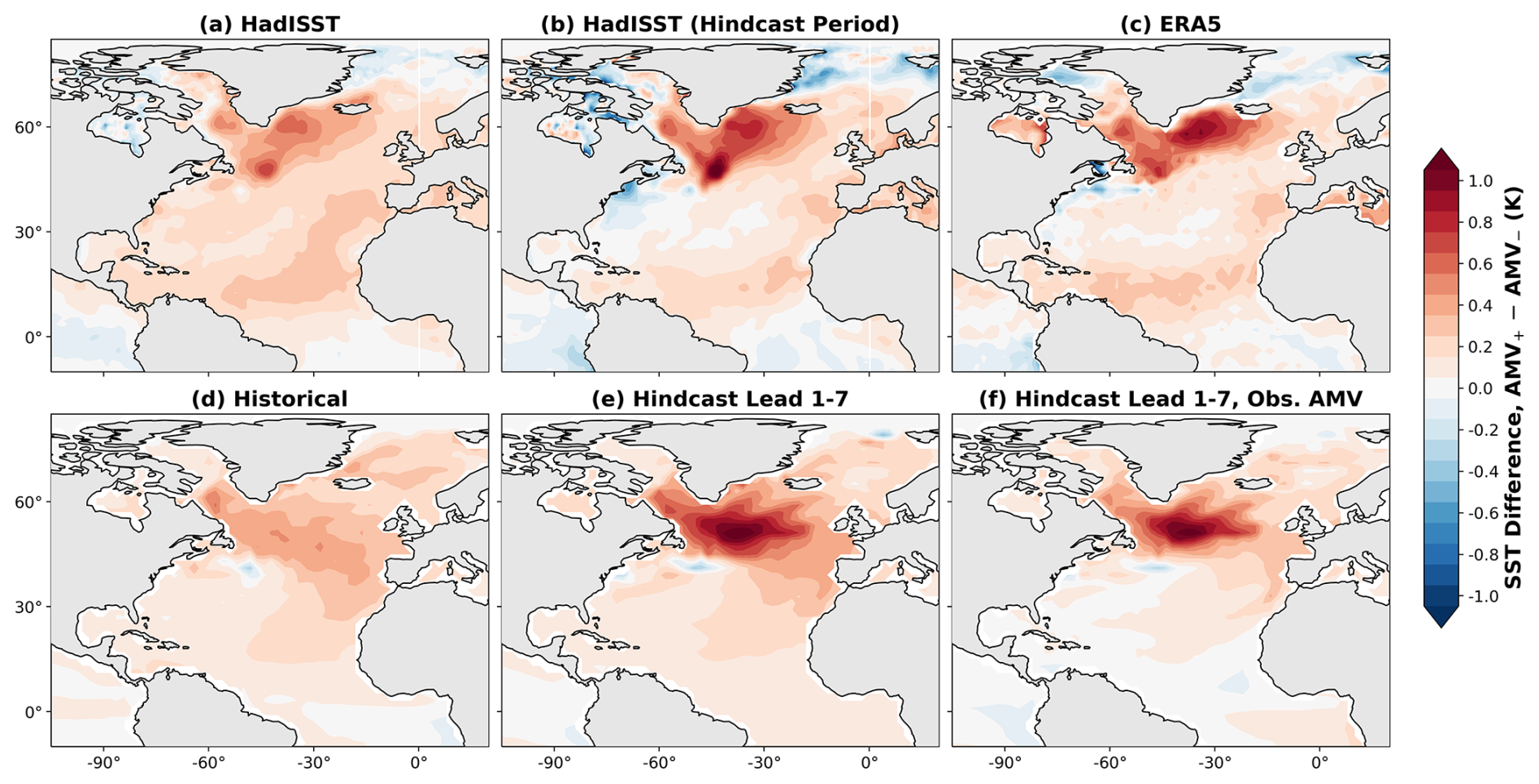
Figure 1 Patterns of 7 year mean AMV SSTs in observations, reanalysis and model experiments. Composite difference between SSTs during positive and negative AMV using SSTs and AMV index from (a) HadISST; (b) HadISST during the period of the decadal hindcasts only; (c) ERA5 during the hindcast period; (d) historical runs using MPI-ESM-LR; and (e) MPI-ESM-LR decadal hindcasts. (f) as with (e), but using the ERA5 AMV index rather than that of the hindcasts.

3 Summer Atmospheric Response to AMV

Accurate simulation of SST anomalies associated with AMV are necessary to accurately simulate impacts. Composites differences in positive and negative AMV phase North Atlantic SSTs from different data sources are shown in Fig. 1. The “horseshoe” pattern of SSTs associated with AMV is clearly present in all observational/reanalysis datasets (Fig. 1a–c); there is a strong positive signal in the SPG region south of Greenland and a band of positive SST anomalies in the tropical North Atlantic, along with warm anomalies at mid-latitudes in the eastern North Atlantic whilst in the west at mid-latitudes, anomalies are relatively small. The strongest anomalies are in the SPG region and this is particularly true during the hindcast period.

The historical large ensemble shows a similar pattern in composites defined using model AMV (Fig. 1d), although the SPG response is considerably weaker and with the strongest anomalies centred further south and east compared to observations/reanalysis. The large ensemble hindcast (Fig. 1e) shows a considerably stronger SPG response which is comparable to hindcast period observations/reanalysis, although the tropical signal is weak. This implies that initialisation has constrained the SPG signature of AMV towards that of observations. By using ERA5 to define AMV phases for the hindcast (Fig. 1f), the predictability of AMV SSTs can be assessed. The strong SPG signal remains, suggesting that it is highly predictable (consistent with previous studies, e.g. Borchert et al., 2021). However, the tropical signal vanishes, suggesting that AMV-driven tropical SST anomalies are poorly predicted at lead 1–7. Figure S1 in the Supplement shows correlation skill maps for hindcast SSTs relative to ERA5 and HadISST, and indicates that prediction skill is highest in the SPG region.

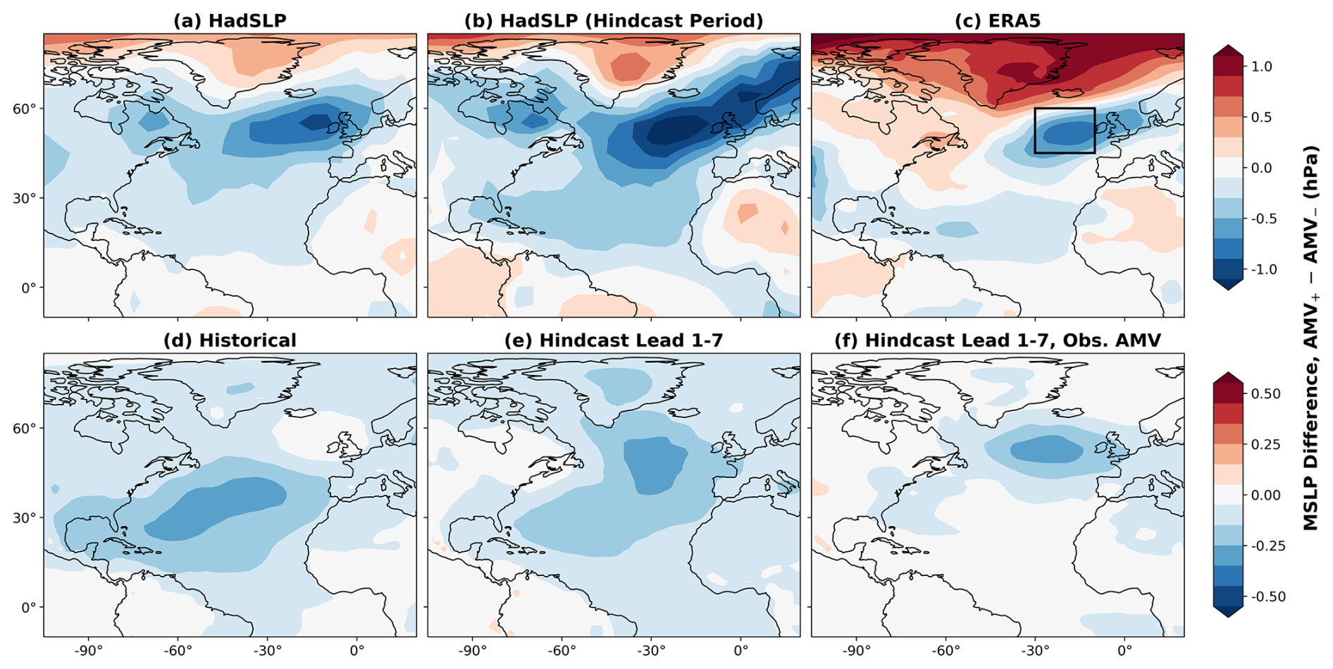
Figure 2 MSLP response to AMV in observations, reanalysis and model experiments. Composite difference in 7 year mean MSLP during positive and negative AMV using MSLP and AMV index from (a) HadSLP/HadISST; (b) HadSLP/HadISST during the common period of the decadal hindcasts and HadSLP only; (c) ERA5 during the hindcast period; (d) historical runs using MPI-ESM-LR and (e) MPI-ESM-LR decadal hindcasts. (f) as with (e), but using the ERA5 AMV index rather than that of the hindcasts. The black box in (c) shows the region used to define East Atlantic MSLP. Note that (a)–(c) and (d)–(f) use different colour scales.

To understand the surface atmospheric response, Fig. 2 shows composites of MSLP for different AMV phases using different data sources. In HadSLP during both the full period and period common to the hindcasts (Fig. 2a and b respectively), the strongest response is a negative anomaly west of Great Britain and Ireland, as previously found in Ghosh et al. (2017). This feature is also present in ERA5 (Fig. 2c), but a comparable positive anomaly exists to its north, resembling the summertime North Atlantic Oscillation (SNAO; Folland et al., 2009). In ERA5 and hindcast period HadSLP, there is a distinct band of negative MSLP anomalies in the tropical North Atlantic, which is a typical low level response to positive SST anomalies in the tropics; this response is weaker in the full HadSLP period.

In the historical MPI-ESM-LR large ensemble (Fig. 2d), the MSLP response to (model) AMV is very different to that of reanalysis/observations. The composite response is negligible in the extratropics where the observed response is strongest. The tropical response is comparable to observations, although it extends further northwards. In the large ensemble hindcast (Fig. 2e), the tropical response is perhaps weaker than in the uninitialised simulations, but a negative pressure anomaly comparable to that in Ghosh et al. (2017) and Fig. 2a–c is present, although notably weaker than observed. The improved extratropical response compared to the historical ensemble is consistent with the difference in SSTs found in Fig. 1. When defining based on ERA5 AMV, the hindcast MSLP composite is consistent with the corresponding SST composite: the tropical signal vanishes but the extratropical signal remains: a cyclonic anomaly with a position consistent with observations, indicating the potential for predictability albeit with a model signal which is weaker than observed. The standard deviation of 7 year mean EA MSLP is comparable across all data shown in Fig. 2 at between 0.6 and 0.7 hPa, indicating that the HadSLP and ERA5 composite responses explain a considerable proportion of the decadal variability in this region. An anticyclonic anomaly to the north of the cyclonic anomaly is present in HadSLP and ERA5, which is not captured by historical and hindcast simulations.

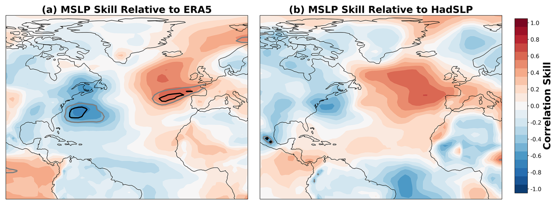
Figure 3 Decadal hindcast skill for MSLP. Temporal correlation between the decadal hindcast ensemble mean MSLP for lead years 1–7 and 7 year rolling mean MSLP from (a) ERA5 and (b) HadSLP. Grey and black contours enclose regions where zero correlation is outside of the 10–90 and 5–95 confidence interval for the correlation skill, respectively. Hindcasts initialised from 1960 to 2005 for HadSLP and to 2016 for ERA5 are considered to cover the respective common periods.

To assess predictability, correlation skill (defined as the Pearson correlation coefficient between the ensemble mean and verifying observations/reanalysis) for hindcast MSLP relative to ERA5 (Fig. 3a) and HadSLP (Fig. 3b) was computed. Note that as HadSLP does not extend as far as ERA5 and the hindcasts, the years used in Fig. 3a and b are not identical, although most of the differences are present when using only the HadSLP/hindcast common period (not shown). The highest skill levels are to be found off the west coast of Europe, where the negative MSLP response to AMV is found. This skill relative to ERA5 is highly significant in some regions. In the western North Atlantic, there are regions of negative skill, which has particularly high magnitude and is significant in ERA5. It is not clear if (and if so, how) this relates to AMV, but the high significance implies potential for predictability, that is nonetheless not realised by the MPI-ESM-LR hindcasts due to model error. In the tropics, MSLP skill is generally lower and differs depending on the observational reference used.

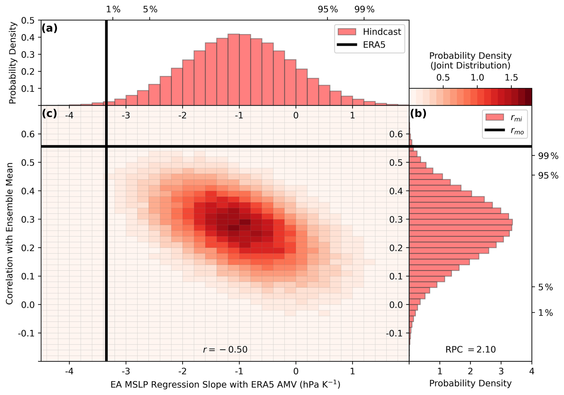
Figure 4 Teleconnection strength deficiencies lead to signal-to-noise errors. (a) histogram of regression slopes for 100 000 samples of single member East Atlantic (EA) MSLP timeseries with the ERA5 AMV Index, along with the same slope but for ERA5 EA MSLP (black line). (b) histogram of correlations r_mi of sampled hindcast member EA MSLP with ensemble mean EA MSLP, along with the correlation between ERA5 and the ensemble mean (black line). (c) joint histogram for the sampled hindcast member statistics in (a) and (b). Black lines in (a) and (b) extend in to (c). In (a) and (b), cumulative 1 %, 5 %, 95 % and 99 % levels for the histograms are shown. All fields are 7 year JJA means, with hindcasts initialised from 1960 to 2016 inclusive considered to cover the full common period.

Although the hindcasts are capable of predicting EA MSLP, the response to AMV is nonetheless weak. Fig. 4a shows the histogram of regression slopes for sampled single member timeseries of EA MSLP with the ERA5 AMV index. Despite considerable spread, the regression slope for ERA5 EA MSLP is more negative/stronger than 99 % of sampled hindcast slopes. An underestimated response to a predictable driver can contribute to the signal-to-noise paradox, which is examined in Fig. 4b. The correlation between ensemble mean EA MSLP and that of sampled individual members r_mi is calculated and plotted as a histogram; the ensemble mean correlation skill r_mo computed relative to ERA5 is greater than 99 % of all values of r_mi, and the ratio of predictable components (RPC) is above 2, suggesting that the reliability issues which define the signal-to-noise paradox are present with high significance. Finally, Fig. 4c shows the joint distribution (as a 2-dimensional histogram) of the EA MSLP/ERA5 AMV regression slopes and r_mi values. The sloped pattern demonstrates that the two quantities are related, with a correlation of −0.50, demonstrating that the weak atmospheric response to AMV relates to the signal-to-noise paradox for summer decadal prediction. Overall, Fig. 4 demonstrates that the EA MSLP response to AMV is underestimated in MPI-ESM-LR decadal hindcasts and as a consequence, the ensemble signal-to-noise ratio is significantly lower than that of observations, affecting the reliability of the hindcasts.

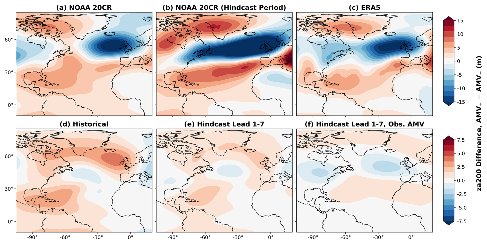
Figure 5 200 hPa geopotential height response to AMV in reanalyses and model experiments. Composite difference in 7 year mean JJA zonal anomaly geopotential height at 200 hPa during positive and negative AMV using MSLP and AMV index from (a) NOAA 20CR/HadISST; (b) NOAA 20CR/HadISST during the common period of the decadal hindcasts and NOAA 20CR only; (c) ERA5 during the hindcast period; (d) historical runs using MPI-ESM-LR and (e) MPI-ESM-LR decadal hindcasts. (f) as with (e), but using the ERA5 AMV index rather than that of the hindcasts. Note that the zonal mean is removed in each case (see text) and (a–c) and (d–f) use different colour scales.

The upper tropospheric response to AMV is important for downstream impacts. In Fig. 5, composites differences of zonally anomalous 200 hPa geopotential height for positive and negative AMV phases are shown for different data sources. The zonal mean is removed as there are large discrepancies between NOAA 20CR and ERA5 in the zonal mean component, particularly in the tropics/subtropics. The cause of this discrepancy is unclear and it was found to not be an artifact of the detrending method used. The atmospheric response to extratropical heating is often shallow (Hoskins and Karoly, 1981; Gastineau and Frankignoul, 2015; Ghosh et al., 2017). Despite this, the upper tropospheric response in the extratropical eastern Atlantic in NOAA 20CR and ERA5 reanalyses (Fig. 5a–c) appears to be an extension of the negative response at the surface and considerable negative anomalies exist at levels between the surface and 200 hPa in this region (not shown). In this particular region the reanalysis results were found to be the same when the zonal mean is not removed (not shown). In the tropical/subtropical North Atlantic, the upper level response is positive and hence baroclinic through the troposphere, which is typical in response to tropical SST anomalies.

When using model AMV, model composites (Fig. 5d–e) are similar to each other and markedly different from reanalysis. The response resembles a Rossby wave train emanating from the Caribbean, leading to a negative response east/south east of Newfoundland and a positive response in approximately the position of the strong negative response in reanalyses. The hindcast response is weaker than in the historical simulations. The hindcast composite using ERA5 AMV phases (Fig. 5f) shows a weak signal which resembles the reanalysis response in the extratropics. Figure 1f demonstrated that tropical SSTs are poorly predicted by the hindcasts, which likely explains why the tropical-origin Rossby wave response is not present in Fig. 5f. The standard deviation of 7 year mean EA 200 hPa geopotential height is between 13 and 14 m for all data in Fig. 5 except NOAA 20CR for the period common with the hindcasts, which is around 11 m. This indicates that the reanalysis composite responses to AMV explain a large proportion of the variability in this region.

With knowledge of the 200 hPa geopotential height response to AMV found in model experiments, it is useful to re-consider whether the reanalysis responses may also relate to a Rossby wave train from the Caribbean. The response over the Caribbean is similar in reanalyses and model experiments, whilst the extratropical response in reanalyses is likely to at least in-part relate to the surface level response to extratropical diabatic heating. As the hindcast extratropical MSLP response is much weaker than that in observations/reanalyses, it is not surprising that it is less likely to extend to the upper troposphere; furthermore in the case of Fig. 1f where the confounding effect of tropical SST anomalies is reduced, the pattern is remarkably similar, albeit much weaker, to that in reanalyses. It is therefore hypothesised that the upper tropospheric response in reanalyses is some combination of the Rossby wave train response to tropical SSTs which is evident in the model experiments, and the surface response to diabatic heating in the SPG region extending upwards. This hypothesis is tested in the next section.

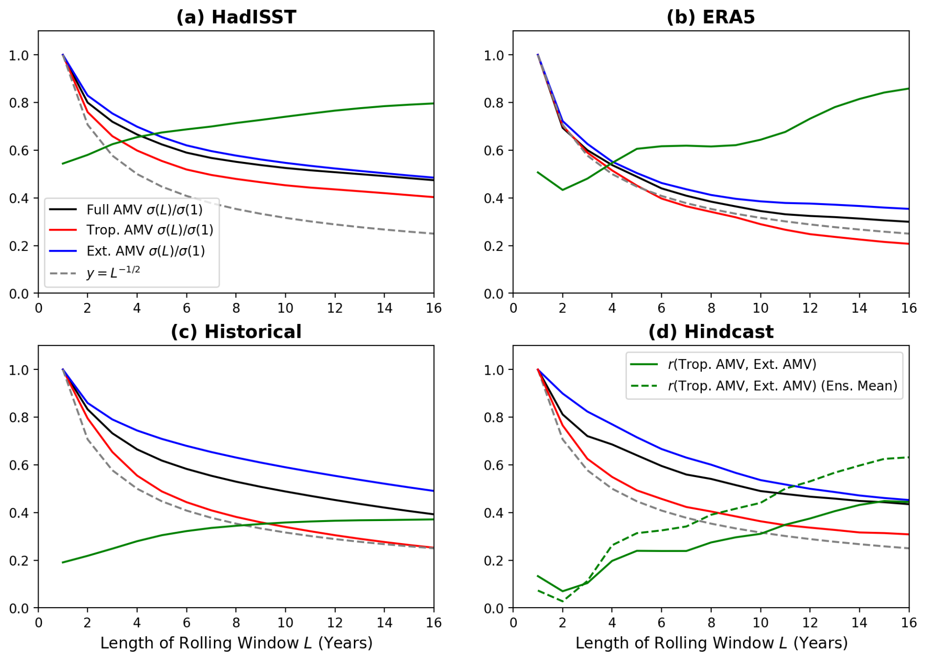
Figure 6 Tropical and extratropical North Atlantic SST variability for different rolling windows. Ratio of rolling mean to interannual standard deviation for the full AMV region and its tropical (south of 30° N) and extratropical (north of 30° N) components in (a) HadISST, (b) ERA5, (c) Historical MPI-ESM-LR simulations and (d) MPI-ESM-LR hindcasts, where each rolling window L is the mean of leads 1 to L. Grey dashed lines show the theoretical relationship for white noise (see Sect. 2). Solid green lines show correlations between tropical and extratropical AMV against rolling window length (calculated as the mean of correlations from individual members), while the dashed green line in (d) shows the same for the hindcast ensemble mean. In all cases, the full period of data availability is used, except only data common to the hindcast period is used for ERA5 (see Sect. 2).

4 Timescale Dependence of Tropical and Extratropical Pathways

Subpolar gyre SST variability is known to have a large multidecadal component associated with AMV (Zhang et al., 2019), whilst considerable interannual variability exists in tropical Atlantic SSTs (Cai et al., 2019). Therefore the relative contributions of the tropics and extratropics to North Atlantic SST variability are likely to depend on the timescale of interest. In Fig. 6, the ratio of standard deviations of rolling-averaged SSTs to that of interannual SSTs is shown for different rolling window lengths, using the full, tropical and extratropical AMV indices as defined in Sect. 2. Low-frequency variability beyond that of white noise exists for the full AMV region in all datasets. In all cases, extratropical North Atlantic SSTs have a greater ratio than the full region, and in turn tropical SSTs have a lower ratio than the full region. It should therefore be expected that in both model experiments and reanalyses, the longer the rolling window used, the larger the relative contribution of extratropical SSTs to AMV region variability. As a result, it is expected that the diabatic heating response to extratropical SSTs should play an increasingly important role in the upper level atmospheric response with increasing rolling window length.

The coupling of tropical and extratropical North Atlantic SSTs depends on timescale. Figure 6 also shows correlations between tropical and extratropical AMV for different rolling window lengths. In all cases, the correlation tends to increase with increasing rolling window length; this may be explained by direct forcing of the tropical Atlantic by the extratropical Atlantic on multidecadal timescales (Brown et al., 2016; Drews and Greatbatch, 2017; Senapati et al., 2024), with remote forcing driving interannual variability (Cai et al., 2019, and references therein). The HadISST and ERA5 correlations are large, demonstrating that the extratropical and tropical SSTs are strongly coupled; this, alongside the relatively short length of data availability, means that it is difficult to separate the effects of tropical and extratropical SSTs by defining composites based on them rather than the full AMV index. In both the historical and hindcast simulations, the tropical-extratropical SST correlations are much lower than in observations, although in both cases the correlation increases with rolling window length as in observations.

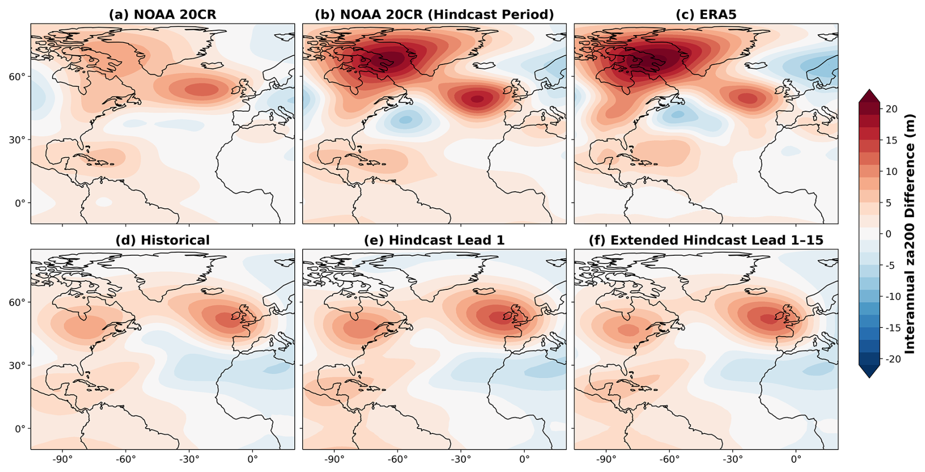
Figure 7 Year-on-year 200 hPa geopotential height response to AMV index variability in reanalysis and MPI-ESM-LR model experiments, where year-on-year variability is computed as half the difference between consecutive years (see Sect. 2 for more details). Composite difference in 200 hPa geopotential height during positive and negative interannual AMV index years using geopotential height and SSTs from (a) NOAA 20CR/HadISST; (b) NOAA 20CR/HadISST during the common period of the decadal hindcasts and NOAA 20CR only; (c) ERA5 during the hindcast period; (d) historical runs using MPI-ESM-LR, (e) MPI-ESM-LR decadal hindcasts for lead year 1 and (f) single years for leads 1 to 15 in the 16 extended length members of the MPI-ESM-LR decadal hindcasts. Note that the zonal mean is removed in each case, as with the 7 year rolling mean results shown in Fig. 5.

The timescale dependence of tropical and extratropical contributions to North Atlantic SST variability implies that the atmospheric circulation is also likely to depend on timescale. Figure 7 shows the composite difference response of zonally anomalous geopotential height to year-on-year AMV region SST variability. Year-on-year variability is computed as half of the difference between successive summers, in order to filter out multi-year variability (see Sect. 2 for details). Remarkably, a Rossby wave train response emanating from the Caribbean like that found using 7 year rolling means in model experiments (see Fig. 5) is found in all reanalyses and model experiments. This implies that this Rossby wave response is a component of the overall atmospheric response to AMV in reality as well as in model experiments, but it is only the dominant component on the 7 year timescale for the model case. The strength of associated geopotential height anomalies are comparable in all data sources. The zonal mean component was found to be similar amongst reanalyses (not shown), but zonal anomalies are used for consistency with Fig. 5. For the hindcast, results for both lead 1 only and all individual leads up to lead 15 are shown (Fig. 7e and f respectively). There are no major differences, demonstrating that this feature of the hindcast atmospheric response to North Atlantic SSTs is not dependent on lead time.

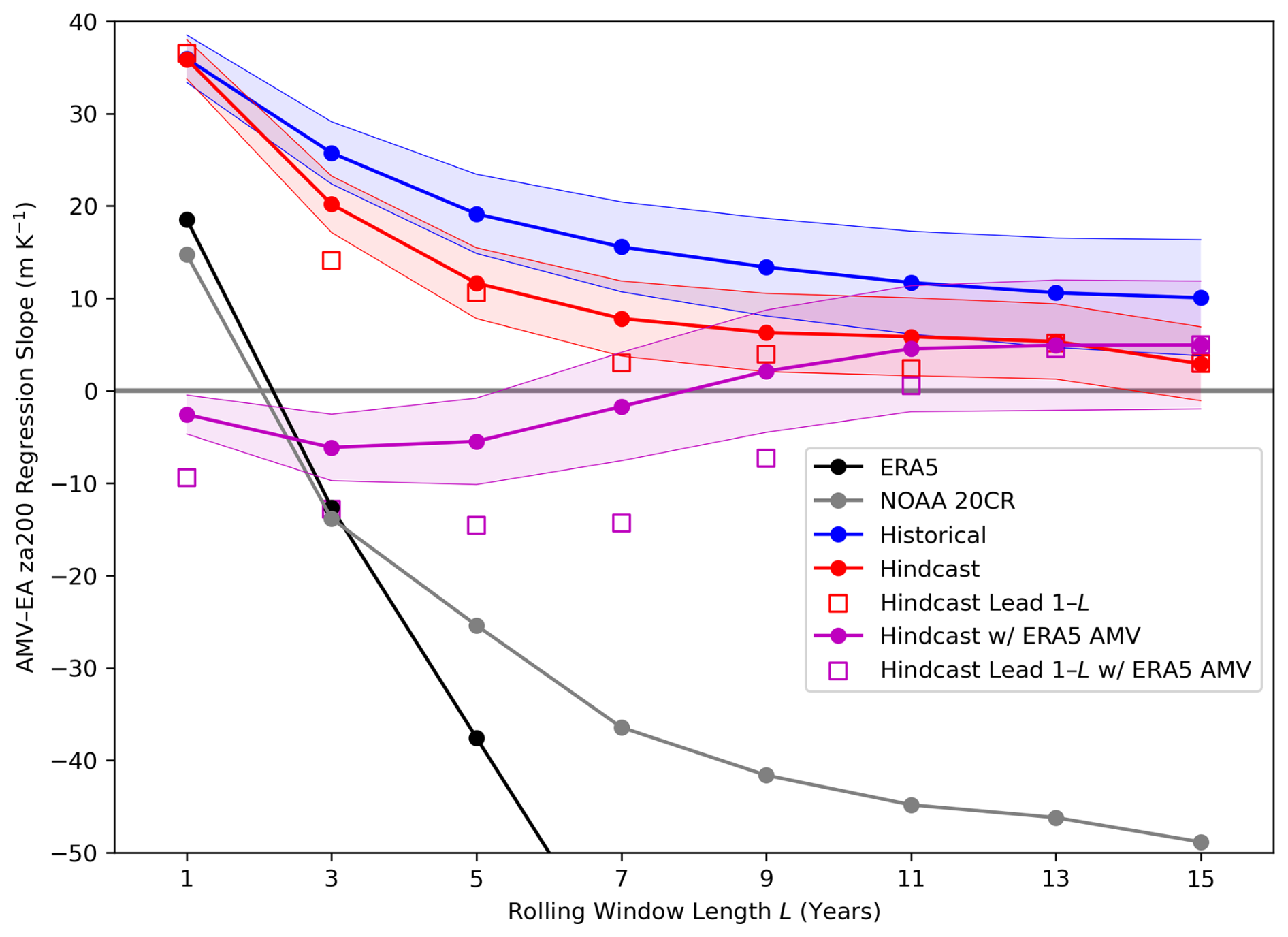
Figure 8 Regression slope between AMV and EA zonally anomalous 200 hPa geopotential height for different rolling window lengths L. Black: ERA5; Grey: NOAA 20CR with HadISST AMV; Blue: MPI-ESM-LR historical simulations; Red: MPI-ESM-LR hindcasts, for all leads (line and filled circles) and lead 1–L (squares); Purple: Hindcasts with ERA5 used for AMV, for all leads (line and filled circles) and lead 1–L (squares). Where the values are for all leads, values are computed individually for each lead, and then averaged. Shaded red and purple regions show the 5–95 confidence interval for the hindcasts at all leads with hindcast and ERA5 AMV respectively, computed as the mean value ± the standard error of slopes from individual member timeseries scaled by 1.644. The shaded blue region shows the 5–95 confidence interval for the historical simulations, computed in the same manner. An alternative version showing the full curves for reanalyses can be found in the Supplement (Fig. S2).

As the 200 hPa geopotential height response to North Atlantic SSTs depends on timescale in reanalyses, it is useful to understand whether the negative response to AMV appears in the model on sufficiently long timescales. Figure 8 shows the regression slope for EA zonal anomaly 200 hPa geopotential height against the AMV index for different rolling window lengths and using different data sources. Only the 16 extended length ensemble members are considered for the hindcasts, and up to lead year 15 is used; results up to lead year 10 are robust when using the full ensemble (not shown). Consistent with Figs. 5 and 7, for single years the slope is positive in ERA5 and NOAA 20CR reanalyses, but becomes increasingly negative with increased rolling window length L. The mean regression slope in historical and hindcast simulations is positive for all rolling window lengths tested (up to 15 years), but in both cases, there is a robust decrease in the regression slope with increased rolling window length, and for all multiyear rolling window lengths, the hindcast slope is significantly lower than that of the historical simulations. By including all leads – for rolling window length L=1, leads 1 to 15 are used, for L=3, leads 1–3, 2–4 up to 13–15 are used, and so on – it is shown that the dependence on rolling window length in the hindcasts is not caused by the inclusion of longer leads with longer rolling windows. Leads 1–L (i.e. the first L summers) are also shown; for L=3 and L=7, the slope is significantly more negative than when considering all leads, demonstrating that the differences are greater at short leads; note that as L tends towards 15, the red squares (lead 1–L) and red circles (all leads) necessarily converge. The y axis limits of Fig. 8 are chosen to highlight model behaviour; an alternative version showing the full curves for reanalyses can be found in the Supplement (Fig. S2).

Figure 8 also shows the hindcast regression slopes using ERA5 AMV. This is the component of the response which relates to skilfully predicted AMV SSTs. When considering all leads, the slopes are significantly less than zero for rolling window lengths of 3, 5 and 7 years, whilst the lead 1–L slope is significantly more negative than for all leads for L from 1 to 9. This is consistent with the skilfully predicted SPG SSTs and poorly predicted tropical SSTs demonstrated in Fig. 1f (and Fig. S1): the response using ERA5 AMV is negative as expected in response to SPG SSTs, and the skill is likely to be highest at short leads.

As the regression slope reduces with increased rolling window length in both hindcasts and historical simulations, it is possible that the model can simulate the upwards extension of the surface level response to extratropical diabatic heating seen in reanalyses, but that it is too weak to play a dominant role in the overall upper tropospheric response to AMV. However, the fact that the regression slope remains positive means that the possibility that the response merely weakens with no opposing mechanism can't be ruled out. The regression slopes using ERA5 AMV allow us to extract the response to extratropical SSTs, exploiting the fact that the (multi-year) SST skill is lower in the tropics. The hindcast regression slope with ERA5 AMV is negative at shorter leads (when skill is highest), suggesting that the model can simulate the response to upper tropospheric response to extratropical diabatic heating seen in reanalyses, but that is extremely weak and so the tropical Rossby wave mechanism plays the dominant role in the response to AMV, even at decadal timescales.

Overall, the observed EA 200 hPa geopotential height response to North Atlantic SST anomalies is positive on interannual timescales, but becomes negative in reanalyses for multiyear windows due the increasing importance of extratropical SSTs relative to tropical SSTs. Due to the weaker/shallower response to extratropical diabatic heating, the hindcast and historical response remains positive for all rolling window lengths considered. However, the hindcast response to the ERA5 AMV index is negative for rolling window lengths up to 9 years, due to skilful prediction of extratropical SSTs at these leads.

5 Discussion and conclusions

The capability of MPI-ESM-LR historical and decadal hindcast simulations at capturing the atmospheric response to Atlantic Multidecadal Variability (AMV) – as well as SST anomalies associated with AMV – was tested. We find that both can capture the typical “horseshoe” pattern of SSTs, but only the hindcasts accurately simulate the strength of subpolar gyre (SPG) SST anomalies. Whilst the SPG response in hindcasts is present when defining composites using ERA5 AMV phases, the tropical SST response largely vanishes, indicating predictability in the extratropics but not in the tropics. The previously reported negative EA MSLP response to AMV during boreal summer was found in observations and reanalyses, which is associated with diabatic heating due to subpolar gyre SST anomalies. This response is not present in the historical simulations, but it is present – although with underestimated amplitude – in the hindcasts, in agreement with the differences in SST anomalies. This response is also found in the hindcasts when using ERA5 AMV phases, suggesting that this response is predictable; the correlation skill between the hindcast ensemble mean and observational references was computed which further demonstrated predictability in the extratropical North Atlantic.

The upper tropospheric (200 hPa) geopotential height response to AMV in MPI-ESM-LR historical and hindcast simulations was also analysed and compared to reanalyses. The negative EA MSLP response was found to extend upwards to this level in reanalyses. Modelled responses are consistent amongst historical and hindcast simulations, and resemble a Rossby wave train emanating from the Caribbean and leading to a positive anomaly in the extratropical eastern North Atlantic. The positive anomalies in the Caribbean which appear to be the origin of the Rossby wave train exist in the reanalyses, leading to the hypothesis that the upper tropospheric reanalysis response to AMV is a combination of the extratropical surface response due to diabatic heating extending upwards, and the tropical-to-extratropical Rossby wave train evident in model simulations.

By varying the number of years used for rolling means, it becomes clear that the relative contribution to AMV SSTs from the extratropics compared to the tropics increases for longer rolling means, indicating a larger proportion of low-frequency variability in the extratropics. As the upper tropospheric response to AMV in reanalyses is hypothesised to consist of two components with one due to tropical SSTs and one due to extratropical SSTs, the 200 hPa geopotential height response is investigated for interannual North Atlantic SST variability. In this case, both the reanalysis and model responses to AMV region SSTs resemble the modelled response to 7 year rolling mean AMV SSTs, highlighting the importance of tropical SST anomalies at shorter timescales, and supporting the hypothesis that the model 7 year Rossby wave response is a component of the reanalysis response. The regression slope of the AMV index on EA 200 hPa geopotential height is calculated for different data sources and rolling window lengths, and a robust reduction in the slope (to negative levels in the case of reanalyses) with increasing rolling window length is found, with a larger reduction in the decadal hindcasts compared to the historical simulations. Furthermore, the predictable part of the hindcast slope (calculated by regressing against ERA5 AMV) is found to have the correct sign for rolling windows lengths from 3 to 9 years. However, this is likely to relate to higher prediction skill for extratropical SSTs compared to tropical SSTs at decadal timescales, and even when using 15 year means the hindcast response to AMV remains positive despite the reduction in slope with increased rolling window length.

The two opposing mechanisms that link summertime AMV index SSTs to East Atlantic 200 hPa geopotential height can be summarised as follows:

• A tropical-origin mechanism, in which warm anomalies in the tropical Atlantic lead to rising in the upper troposphere, causing a Rossby wave train from the Caribbean to the extratropical eastern Atlantic, with positive geopotential height anomalies to the west of Great Britain and Ireland. In reanalyses, this dominates on interannual timescales, when tropical SST variability dominates overall North Atlantic SST variability. MPI-ESM-LR hindcasts and historical simulations can simulate this mechanism.

• An extratropical-origin mechanism, in which diabatic heating associated with warm subpolar gyre SST anomalies leads to a low pressure anomaly in the extratropical eastern Atlantic. In reanalyses, this extends to the upper troposhere and dominates on decadal timescales, when extratropical SST variability dominates. Historical simulations do not capture the surface response whilst it is captured but severely underestimated in hindcasts, and with the tropical-origin mechanism continuing to dominate in the upper troposphere even on 15-year timescales.

Skilful prediction but with underestimated strength of predictable signals is a common phenomenon in the North Atlantic-Europe sector known as the “signal-to-noise paradox” (Scaife and Smith, 2018). By sampling individual member hindcasts we find that the reliability errors which define the signal-to-noise paradox are present in MPI-ESM-LR decadal predictions of JJA East Atlantic MSLP, and that these errors are closely linked to the underestimated atmosperic response to AMV.

With an 80 member hindcast, it has been possible to demonstrate robust MSLP predictability in the region where the observed response to AMV is strongest, despite (a) the weak amplitude of the model response to AMV in this region and (b) the limited degrees of freedom available to assess skill given the short hindcast period. Unless the causes of the signal-to-noise paradox are identified and eliminated, large ensemble forecasts which are post-processed to address signal-to-noise deficiencies are necessary in order to predict summertime decadal variability, including surface impacts. It is notable that the Rossby wave mechanism does not appear to be underestimated in MPI-ESM-LR simulations (except where tropical SST variability is underestimated in the decadal hindcasts); this may be relevant to understand the causes of the signal-to-noise paradox. However, the fact that one mechanism is underestimated whilst the other is not means that skill is reduced where they interfere in the upper troposphere, which is an issue which cannot be easily rectified by increased ensemble size and/or post-processing of forecasts.

The dominance of the response to extratropical diabatic heating in the upper troposphere in reanalyses suggests that the impact of heating associated with SPG SSTs is less shallow than previously reported in Ghosh et al. (2017), but at 7 year timescales it is weak and baroclinic in hindcasts. Ossó et al. (2020) identify a summertime atmospheric response to seasonal springtime Gulf Stream SST anomalies which is equivalent-barotropic in nature, which they attribute to reinforcement through ocean-atmosphere coupling. As with the response to diabatic heating in this study, this response was found to be present but weak in models and hence was identified as potentially relevant to the signal-to-noise paradox; furthermore, model deficiencies were associated with underestimated ocean-atmosphere coupling. Baroclinic anomalies can also lead to stronger, sustained barotropic anomalies through eddy feedback (e.g. O'Reilly and Czaja, 2015), which has also been found to be deficient in models and linked to the signal-to-noise paradox (Hardiman et al., 2022). The role of positive ocean-atmosphere and eddy feedbacks for the observed summer atmospheric response to AMV warrants further study. In particular, MPI-ESM-LR has an atmospheric resolution which is coarse relative to other Decadal Climate Prediction Project models (DCPP; Boer et al., 2016), and recent studies have identified that increased atmospheric and/or oceanic resolution can improve the strength of predictable signals due to improved representation of mesoscale weather phenomena and ocean eddies (Krüger et al., 2026; Scaife et al., 2019; Wills et al., 2024; Yeager et al., 2023; Zhang et al., 2021). It should be noted that the largest improvements in these studies involve resolutions beyond the range of DCPP simulations; nonetheless whether other decadal prediction systems exhibits yield similar results, and whether there is any resolution dependence on model performance warrants further study.

The MPI-ESM-LR hindcasts analysed in this study use full-field initialisation (Brune and Baehr, 2020) in the ocean and atmosphere, meaning that they drift from an unbiased (relative to the initialisation data) to a biased state during the model integration. Atmospheric biases typically develop quickly relative to decadal timescales, but noticeable oceanic drifts may persist for several years before stabilising (Hermanson et al., 2018; Polkova et al., 2023). Both biases and drifts interfere with predicted anomalies, but Polkova et al. (2023) found that decadal hindcasts using full-field initialisation (drifts but with reduced biases) as opposed to anomaly-only initialisation (reduced drift but with a larger bias) had higher prediction skill for SPG SSTs. Additionally, it should be noted that the slower oceanic model drift can be a direct result of integrating the already-developed atmospheric biases, meaning that there is spurious transfer of heat between the ocean and atmosphere (Sanchez-Gomez et al., 2016); this is likely to have an impact on the predicted atmospheric response to oceanic forcing. Whilst we do not investigate biases in this study, the existing literature demonstrates the necessity for targeted effort to reduce model biases in both the ocean and atmosphere in order to maximise prediction skill.

The atmospheric response to subpolar gyre diabatic heating has previously been identified as leading to increased precipitation in northwestern Europe and increased temperatures in central Europe (Ghosh et al., 2017). The aim of this study has been to understand mechanisms behind the summer atmospheric response to AMV and the capability of MPI-ESM-LR model experiments to simulate and predict them; further work is necessary to understand whether models are capable of simulating their surface impacts over Europe and other land regions. The forced trend was removed throughout this study in order to focus on the decadal component of the overall variability, but it is necessary to include the trend in operational prediction of near-term North Atlantic-Europe climate. Recent work has found signal-to-noise errors in the wintertime North Atlantic circulation response to external forcing (Blackport and Fyfe, 2022; Klavans et al., 2021), and so understanding whether this is also an issue during summertime warrants further study, including whether North Atlantic SST trends play a role.

To summarise, the surface level decadal atmospheric response to AMV in the North Atlantic-Europe (NAE) sector during summertime is dominated by a low pressure anomaly to the west of Great Britain and Ireland. This response is a result of diabatic heating due to subpolar gyre SST anomalies, and it is captured by a large ensemble of MPI-ESM-LR decadal hindcasts, resulting in statistically significant MSLP skill. Despite this, the amplitude of the surface level response is strongly underestimated in MPI-ESM-LR decadal hindcasts, which is consistent with the “signal-to-noise paradox” issue in NAE sector climate prediction. The upper level response in reanalyses can be explained by the surface level response extending upwards, whilst in hindcast and historical simulations, the dominant response is a Rossby wave train associated with tropical SST anomalies. By adjusting rolling window lengths between 1 and 15 years, it becomes clear that both the high-frequency tropical Rossby wave and low-frequency extratropical diabatic heating response exist in observations and reanalyses, but deficiencies in the strength of the surface level response in hindcasts means that its role at upper levels is hard to discern in the presence of the opposing tropical Rossby wave response. Overall, this study demonstrates the existence of dynamically-driven skill for decadal prediction of European summers, which is best realised using large ensembles and may be enhanced further by future model improvements.