Ensemble design for seasonal climate predictions: studying extreme Arctic sea ice lows with a rare event algorithm

Initialized ensemble simulations can help identify the physical drivers and assess the probabilities of weather and climate extremes based on a given initial state. However, the significant computational burden of complex climate models makes it challenging to quantitatively investigate extreme events with probabilities below a few percent. A possible solution to overcome this problem is to use rare event algorithms, i.e. computational techniques originally developed in statistical physics that increase the sampling efficiency of rare events in numerical simulations. Here, we apply a rare event algorithm to ensemble simulations with the intermediate-complexity coupled climate model PlaSim-LSG to study extremes of pan-Arctic sea ice area reduction under pre-industrial greenhouse gas conditions. We construct four pairs of control and rare event algorithm ensemble simulations, each starting from four different initial winter sea ice states. The rare event simulations produce sea ice lows with probabilities of 2 orders of magnitude smaller than feasible with the control ensembles and drastically increase the number of extremes compared to direct sampling. We find that for a given probability level, the amplitude of negative late-summer sea ice area anomalies strongly depends on the baseline winter sea ice thickness but hardly on the baseline winter sea ice area. Finally, we investigate the physical processes in two trajectories leading to sea ice lows with conditional probabilities of less than 0.001 %. In both cases, negative late-summer pan-Arctic sea ice area anomalies are preceded by negative spring sea ice thickness anomalies. These are related to enhanced surface downward longwave radiative and sensible heat fluxes in an anomalously moist, cloudy and warm atmosphere. During summer, extreme sea ice area reduction is favoured by enhanced open-water-formation efficiency, anomalously strong downward solar radiation and the sea ice–albedo feedback. This work highlights that the most extreme summer sea ice conditions result from the combined effects of preconditioning and weather variability, emphasizing the need for thoughtful ensemble design when turning to real applications.

1 Introduction

Anthropogenic emissions of greenhouse gases have contributed to the loss of Arctic sea ice during the last 45 years (Notz and Marotzke, 2012; Stroeve and Notz, 2018; Gregory et al., 2002; Ding et al., 2017). Despite the steadily increasing rate of greenhouse gas concentrations (Meinshausen et al., 2017), the decline of the pan-Arctic sea ice area is non-linear, and internal climate variability and feedback mechanisms have been shown to modulate the downward trend of the sea ice (Ding et al., 2017; Baxter et al., 2019; Ono et al., 2019; Francis and Wu, 2020; Tietsche et al., 2011; England et al., 2019). Accelerated decline of the late-summer sea ice area occurred from the mid-2000s to 2012, resulting in record reductions of sea ice area compared to the trend line in 2007 and 2012.

Various studies attributed the 2007 and 2012 drastic sea ice loss events both to climate change via preconditioning through the ongoing winter sea ice thinning and to internal climate variability via particular weather and climate events during the melting season (Lindsay et al., 2009; Kauker et al., 2009; Zhang et al., 2008, 2013; Parkinson and Comiso, 2013; Kirchmeier-Young et al., 2017). While progress has been made in quantifying the relative contributions of anthropogenically forced vs. internal climate variability to the observed downward trend of the sea ice cover in the Arctic (e.g. Ding et al., 2017; England et al., 2019), their relative contributions to extreme sea ice loss events such as observed in 2007 and 2012 are uncertain (Kirchmeier-Young et al., 2017; Ono et al., 2019). By applying an extreme event attribution analysis to ensemble simulations with the Second Generation Canadian Earth System Model (CanESM2), Kirchmeier-Young et al. (2017) concluded that a sea ice low with an amplitude as observed in 2012 (i.e. a 2012-like sea ice area anomaly relative to the observed 1981–2010 mean) would have been extremely unlikely to occur without global warming. A substantial contribution of internal climate variability to the 2007 and 2012 events is turn evidenced by the fact that, despite ongoing global warming, summer sea ice conditions are still above the 2012 minimum (Baxter et al., 2019; Francis and Wu, 2020).

Different drivers of anomalously low summer Arctic sea ice area were discussed in the literature. These include enhanced North Atlantic and Pacific oceanic heat transport (Årthun et al., 2012; Woodgate et al., 2010), the positive and negative phases of the winter and summer Arctic Oscillation (AO) (e.g. Rigor et al., 2002; Ogi et al., 2016), reduced cloudiness during summer (Schweiger et al., 2008), and increased surface downward longwave radiation related to enhanced poleward atmospheric moisture transport during spring (Kapsch et al., 2013, 2019). In 2007, sea ice reduction was favoured by enhanced inflow of warm Pacific water through the Bering Strait (Woodgate et al., 2010) and by anomalously persistent southerly winds in the Pacific sector associated with the Arctic Dipole Anomaly (ADA) pattern (Wang et al., 2009; Lindsay et al., 2009; Overland et al., 2012; Kauker et al., 2009). In 2012, a summer storm contributed to enhanced sea ice reduction by leading to increased bottom melt via anomalously strong vertical mixing in the oceanic boundary layer (Guemas et al., 2013; Zhang et al., 2013).

Even though the physical drivers of individual extremes of Arctic sea ice reduction have been suggested, their quantitative statistical analysis is hampered by the small number of extreme events that can be sampled from observations and numerical simulations. Likewise, it is the small number of events in the lower tail of the distribution of sea ice area values that makes it challenging to quantify the probability of a 2012-like sea ice low event for a given background climate and for a given initial condition. The record of satellite-based sea ice observations includes only a few annual sea ice minima with orders of magnitude comparable to the ones in September 2007 and 2012 (Fetterer et al., 2017). Moreover, the large computational cost of complex climate models makes it unrealistic to run ensembles with a few thousands of trajectories and to quantitatively study extreme events with probabilities of less than 1 %. The use of multiple models instead of one single model would increase the computational cost even further. One workaround is to estimate these very small probabilities with extreme value theory models (Coles, 2001). However, even when applicable, these methods only provide a statistical extrapolation of the probabilities and do not provide information on the dynamics. A better understanding of the precursors of extremes of summer Arctic sea ice reduction and a more precise estimate of their probabilities are in turn crucial to improve seasonal predictions of these events and to assess their risk of occurrence under different climate change scenarios.

In this work, we study extremely negative summer pan-Arctic sea ice area anomalies using initialized ensemble simulations with the intermediate-complexity coupled climate model PlaSim-LSG under pre-industrial greenhouse gas conditions. We investigate the statistical properties of extreme summer sea ice lows as a function of different initial winter states and examine the physical drivers favouring extremes of sea ice area reduction within a single melting season. In order to improve the sampling of extreme sea ice loss events, we use a rare event algorithm. Rare event algorithms are computational techniques developed in statistical physics to improve the sampling efficiency of rare events in numerical simulations (e.g Ragone et al., 2018; Ragone and Bouchet, 2020, 2021; Sauer et al., 2024a). Compared to conventional numerical simulations with the same computational cost, rare event algorithms enable the number of simulated extreme events to be increased by several orders of magnitude while preserving the dynamical consistency of the model. In this way, these techniques allow the uncertainty of probability and return time estimates and of conditional statistics on extreme events (e.g. composites) to be reduced compared to conventional simulation strategies and ultra-rare events to be generated that are very unlikely to be observed using direct sampling. Rare event algorithms were introduced in the 1950s (Kahn and Harris, 1951) and have been used since for a wide range of applications (for an overview and the mathematical analysis, see for example, Del Moral, 2004; Giardina et al., 2011; Grafke and Vanden-Eijnden, 2019). Recently, some of these techniques have been applied in climate science and in fluid dynamics to study heat waves (Ragone et al., 2018; Ragone and Bouchet, 2020, 2021), midlatitude precipitation (Wouters et al., 2023), tropical storms (Plotkin et al., 2019; Webber et al., 2019), weakening and collapse of the Atlantic Meridional Overturning Circulation (AMOC) (Cini et al., 2023), extreme Arctic sea ice lows related to unconditional probability distributions (Sauer et al., 2024a), and turbulence (Bouchet et al., 2018; Grafke et al., 2015; Lestang et al., 2020).

Here we use a genealogical selection algorithm (Ragone et al., 2018; Ragone and Bouchet, 2020, 2021; Sauer et al., 2024a), adapted from Del Moral and Garnier (2005) and Giardina et al. (2011), that is efficient to study persistent, long-lasting events. A first application of this algorithm to study extreme Arctic sea ice lows in the intermediate-complexity coupled climate model PlaSim under pre-industrial greenhouse gas conditions is given in Sauer et al. (2024a). In that study, ensemble simulations with the rare event algorithm were initialized with independent initial conditions sampled from a stationary 3000-year control run such that the statistics of extreme events is related to unconditional probability distributions. In such an approach, the rare event algorithm seeks to oversample trajectories leading to low sea ice states in an absolute sense, i.e. independent from the extent to which the sea ice lows are related to multi-annual fluctuations in the sea ice–ocean system (referred to as “preconditioning” in Sauer et al., 2024a) or driven by the dynamics occurring on intra-seasonal timescales. Here, instead, we use a seasonal climate prediction set-up where an ensemble simulation is initialized from a single initial condition to which a small perturbation is added. The goal of these experiments is to disentangle the roles of the initial condition vs. seasonal-scale fluctuations in favouring the occurrence of extremely negative summer sea ice area anomalies. A similar investigation on the influence of initial conditions on an extreme event, albeit using action minimization instead of a genealogical selection algorithm and applied to extreme tropical cyclones, is performed in Plotkin et al. (2019). Here we perform different ensemble simulations starting from different initial conditions sampled from the same control run as in Sauer et al. (2024a). Since each individual ensemble simulation is initialized from a same, slightly perturbed initial condition, statistical and physical properties of low sea ice states inferred from that ensemble need to be interpreted in terms of conditional probabilities.

Owing to the rare event algorithm, we generate extremely low sea ice summers with conditional probabilities of less than 0.001 %. Likewise, we investigate the impact of different initial conditions on the probabilities and amplitudes of extreme sea ice lows. Finally, we elaborate physical drivers in two trajectories leading to late-summer sea ice lows with probabilities of less than 0.001 %. The paper is structured as follows. In Sect. 2, we present the set-up of the model, the methodology of the rare event algorithm, and the design of control and rare event algorithm ensemble simulations. In Sect. 3, we show that the rare event algorithm improves the sampling efficiency of extreme sea ice lows conditional on starting from a certain initial condition compared to standard control ensemble simulations. We analyse the impact of the initial condition on the probabilities and amplitudes of the extremes. In Sect. 4, we discuss physical processes and conditions in individual trajectories prior to extreme sea ice lows with probabilities with less than 0.001 %. In Sect. 5, we present our conclusions.

2 Materials and methods

2.1 Model and data

All simulations are performed with a coupled set-up of the intermediate-complexity climate model Planet Simulator (PlaSim) version 17 (Fraedrich et al., 2005). This set-up includes a dynamic Large-Scale Geostrophic (LSG) ocean (Maier-Reimer et al., 1993; Drijfhout et al., 1996), a mixed-layer ocean and a thermodynamic sea ice model (PlaSim coupled to LSG is referred to as “PlaSim-LSG” in the following).

The atmosphere is run with a horizontal spectral resolution of T21 (triangular truncation at wavenumber $\mathrm{21}\sim \mathrm{5.625}\mathit{°}\times \mathrm{5.625}\mathit{°}$ on a Gaussian grid), 10 levels up to 40 hPa in the vertical and a computational time step of 45 min. The LSG is configured on a 2.5°×5° staggered E-type grid (Arakawa and Lamb, 1977) in the horizontal, with 22 levels and a maximum ocean depth of 6000 m in the vertical and a computational time step of 5 d. The sea ice model is based on the zero-layer model of Semtner (1976). It computes the sea ice thickness and sea surface temperature evolution from the energy balances at the top and bottom of a sea ice–snow layer. The sea ice–snow layer is assumed to have a linear temperature gradient and to have no capacity to store heat. No sea ice drift is taken into account. The sea ice concentration is binary; i.e. a grid cell is fully sea ice covered or open water. The computational time step in the sea ice and mixed-layer ocean models is 1 d.

PlaSim-LSG is run with a fixed pre-industrial effective CO₂ volume mixing ratio of 280 ppmv. We choose a constant greenhouse gas forcing since we are interested in the statistics and dynamics of Arctic sea ice lows related to internal climate variability under a stationary climate. Solar radiation includes the seasonal cycle but not the diurnal cycle. Each model month is 30 d long.

We use data from a stationary 3000-year control run (Sauer et al., 2024a) and from a set of control and rare event algorithm ensemble simulations (see Sect. 2.2 for more details). We consider the statistics of the pan-Arctic sea ice area

$$\begin{array}{}\text{(1)}& {\displaystyle }{\displaystyle }A\left(t\right)=\sum _{\mathit{\varphi }\ge {\mathit{\varphi }}_{\text{min}}}\sum _{\mathit{\lambda }}{\text{SIC}}_{\mathit{\varphi },\mathit{\lambda }}\left(t\right)\cdot G_{\mathit{\varphi },\mathit{\lambda }},\end{array}$$

where SIC_ϕ,λ(t) is the sea ice concentration at time t in a grid cell centred at latitude ϕ and longitude $\mathit{\lambda },G_{\mathit{\varphi },\mathit{\lambda }}={\int }_{\mathit{\varphi }-\frac{\mathrm{\Delta }\mathit{\varphi }}{\mathrm{2}}}^{\mathit{\varphi }+\frac{\mathrm{\Delta }\mathit{\varphi }}{\mathrm{2}}}{\int }_{\mathit{\lambda }-\frac{\mathrm{\Delta }\mathit{\lambda }}{\mathrm{2}}}^{\mathit{\lambda }+\frac{\mathrm{\Delta }\mathit{\lambda }}{\mathrm{2}}}{R}^{\mathrm{2}}\cos \left({\mathit{\varphi }}^{\prime }\right)\mathrm{d}{\mathit{\lambda }}^{\prime }\mathrm{d}{\mathit{\varphi }}^{\prime }$ is the grid cell area, R is the earth radius, and Δϕ and Δλ are the angular distances between two grid points in the meridional and zonal direction. The summation in Eq. (1) includes all ocean grid boxes north of 40° N (i.e. ${\mathit{\varphi }}_{\text{min}}\cdot \frac{\mathrm{180}\mathrm{°}}{\mathit{\pi }}=\mathrm{40}\mathrm{°}$) with a binary land–sea mask (i.e. a grid cell is either completely ocean or completely land). The annual average, amplitude of the seasonal cycle, and the timing of the annual minimum and maximum of the pan-Arctic sea ice area produced by the model are representative of the observed Arctic sea ice climatology between 1979 and 2015 (cf. Fig. 1a and c of Sauer et al., 2024a, and Fig. S1 in the Supplement of Sauer et al., 2024a). Likewise, PlaSim captures a spring predictability barrier-like structure in the persistence of pan-Arctic sea ice area anomalies similar to the one found in comprehensive climate models (cf. Fig. S1 and Blanchard-Wrigglesworth et al., 2011; Day et al., 2014). Compared to the 1979–2015 climatology available from the Pan-Arctic Ice Ocean Modeling and Assimilation System (PIOMAS), PlaSim represents the pan-Arctic sea ice volume reasonably well during spring and slightly underestimates the sea ice volume during summer (cf. Fig. S2a in the Supplement and p. 207 of Chevallier et al., 2019). Differences in the representation of sea ice in PlaSim-LSG compared to observations and reanalysis data include a delayed melting period, a positive sea ice concentration (SIC) bias from the Greenland to the Kara Sea, a negative SIC bias western of Greenland, and positive sea ice thickness biases around the North Pole and from the Greenland to Kara seas (cf. Fig. 1a and c of Sauer et al., 2024a, Fig. S1 of Sauer et al., 2024a, p. 207 of Chevallier et al., 2019, and Fig. S2b). While overall the differences between the pan-Arctic sea ice area in PlaSim-LSG and in observational data are small compared to the range of sea ice area values available from the Coupled Model Intercomparison Project Phase 6 (CMIP6) models (Notz and SIMIP Community, 2020), the regional sea ice thickness and sea ice concentration biases of PlaSim compared to the derived 1979–2015 climatologies may impact the interpretation of the results. We will discuss this point in Sect. 5.

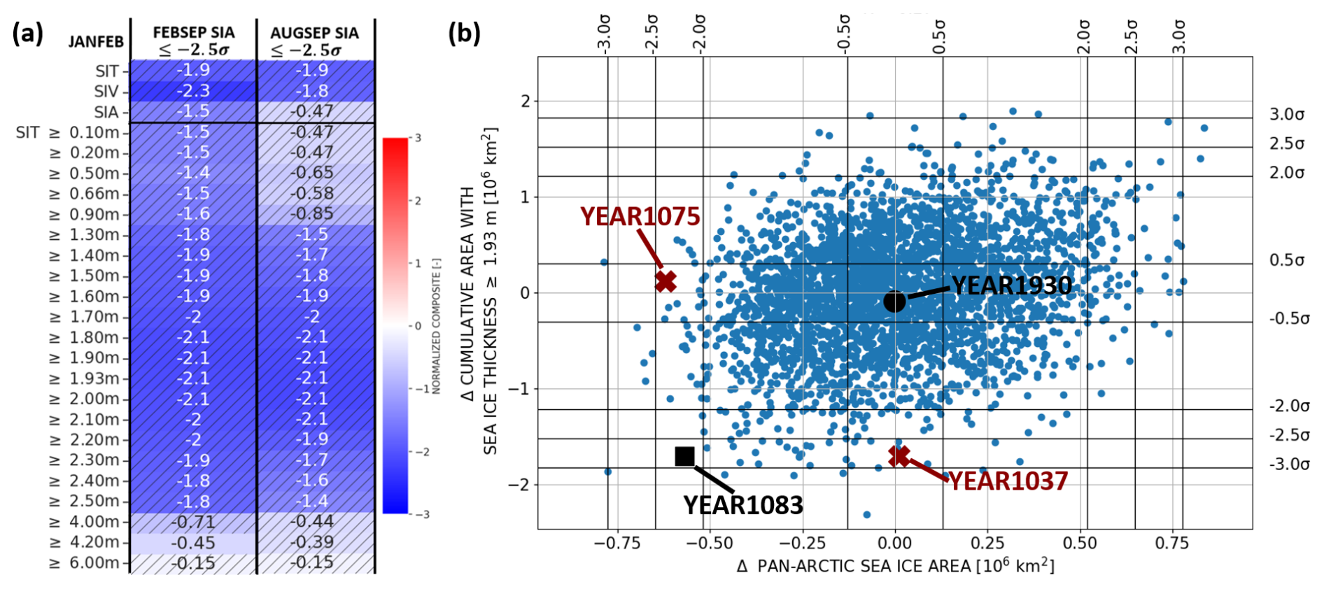
Figure 1 PlaSim-LSG 3000-year control run (Sauer et al., 2024a): (a) Normalized mean anomalies of January–February mean quantities conditional on extreme negative (left) February–September (FEBSEP) and (right) August–September (AUGSEP) mean pan-Arctic sea ice area anomalies equal to or smaller than −2.5 standard deviations. “SIV”, “SIA” and “SIT” are the pan-Arctic sea ice volume, sea ice area and mean sea ice thickness. “SIT ≤ threshold” are anomalies in the cumulative area with sea ice thickness equal to or larger than a critical threshold. Hatching denotes statistical significance at the 5 % level assessed from a two-sided t test applied to five composite estimates after subdividing the 3000-year control run into five 600-member ensembles (see Fig. S4 for more details). (b) Scatter plot of January–February mean anomalies of SIT1.93 vs. pan-Arctic sea ice area including the years from the selected initial conditions.

We study extreme anomalies of February–September and August–September mean pan-Arctic sea ice area. We classify a sea ice area anomaly I^′(t) as extremely negative if $I^{\prime }\left(t\right)\le n{\mathit{\sigma }}_{\text{ctrl}}$, where σ_ctrl is the standard deviation of sea ice area in the control run or in a control ensemble (see Sect. 2.2) and n is a real-valued number. In the following, we will vary n continuously to study an extensive range of extreme event amplitudes.

2.2 Rare event algorithm: methodology and set-up

One key difficulty in the study of climate extremes is the lack of robust statistics as the large computational burden of complex climate models makes it unfeasible to run them long enough to sample a large number of trajectories corresponding to the tail of the distribution of a target observable.

The rare event algorithm presented in recent studies (Giardina et al., 2011; Ragone et al., 2018; Ragone and Bouchet, 2020, 2021; Sauer et al., 2024a) is a genealogical selection algorithm applied on top of an ensemble simulation. It is designed to improve the sampling efficiency of trajectories populating the tail of the distribution of the time average of a target observable A(t). At constant intervals of a resampling time τ_r, we assign to each trajectory a weight. The weight is a function of the time average of the observable during the past interval of duration τ_r for that trajectory. Before simulating the next time window of length τ_r, trajectories with small weights are removed from the ensemble and are substituted by slightly perturbed copies of trajectories with large weights. The algorithm includes a parameter k, which controls the relative amplitude of the weights for given values of the target observable, where the case k=0 would correspond to a regular ensemble simulation. If τ_r is not larger than the decorrelation time of the observable, then the selection will favour the survival of trajectories leading to extreme anomalies of the time average of a target observable such as the pan-Arctic sea ice area (positive for k positive and vice versa). We refer to Ragone et al. (2018), Ragone and Bouchet (2020, 2021), and Sauer et al. (2024a) for more details about the method and present the main outcome here.

We denote X(t) the vector of all model variables at time t and T_a the total simulation time. We consider an ensemble of N trajectories {X_n(t)} ($n=\mathrm{1},\mathrm{2},\mathrm{\dots },N$). Let ${\mathbb{P}}_{\mathrm{0}}\left(\mathit{\right\{}{X}_n\left(t\right){\mathit{\}}}_{\mathrm{0}\le t\le T_a})$ be the probability density of observing a given trajectory X_n(t) from time 0 to time T_a in a direct numerical simulation with the model and ${\mathbb{P}}_k\left(\mathit{\right\{}{X}_n\left(t\right){\mathit{\}}}_{\mathrm{0}\le t\le T_a})$ be the probability density of the same trajectory in an ensemble simulation with the rare event algorithm with a given value of the parameter k. For a large ensemble size N, the relation between the two is given by the importance sampling formula

$$\begin{array}{}\text{(2)}& {\displaystyle }\begin{array}{rl}{\mathbb{P}}_k& \left({\left\{X_n\left(t\right)\right\}}_{\mathrm{0}\le t\le T_a}\right)\underset{N\to \mathrm{\infty }}{\sim }\\ & {\displaystyle \frac{{\mathrm{e}}^{k{\int }_{\mathrm{0}}^{T_a}A\left(\mathit{\right\{}{X}_n\left(t\right)\mathit{\left\}}\right)\mathrm{d}t}}{{\mathbb{E}}_{\mathrm{0}}\left[{\mathrm{e}}^{k{\int }_{\mathrm{0}}^{T_a}A\left(\left\{X_n\left(t\right)\right\}\right)\mathrm{d}t}\right]}}{\mathbb{P}}_{\mathrm{0}}\left({\left\{X_n\left(t\right)\right\}}_{\mathrm{0}\le t\le T_a}\right),\end{array}\end{array}$$

where 𝔼₀ is the expectation value with respect to ℙ₀,A{X_n(t)} the target observable and k a biasing parameter controlling the strength of the selection. Thanks to Eq. (2), the expectation value according to ℙ₀ (the real statistics of the system) of a generic quantity $O\left(\mathit{\right\{}{X}_n\left(t\right){\mathit{\}}}_{\mathrm{0}\le t\le T_a})$ can be estimated from data generated with the algorithm (which are instead distributed according to ℙ_k) as

$$\begin{array}{}\text{(3)}& {\displaystyle }\begin{array}{rl}{\mathbb{E}}_{\mathrm{0}}& \left[O\right(\mathit{\left\{}{X}_n\right(t\left){\mathit{\}}}_{\mathrm{0}\le t\le T_a}\right)]\underset{N\to \mathrm{\infty }}{\sim }\\ & {\displaystyle \frac{\mathrm{1}}{N}}\sum _{n=\mathrm{1}}^N{Z}_k{\mathrm{e}}^{-k{\int }_{\mathrm{0}}^{T_a}A\left(\mathit{\right\{}{X}_n\left(t\right)\mathit{\left\}}\right)\mathrm{d}t}\cdot O\left(\mathit{\right\{}{X}_n\left(t\right){\mathit{\}}}_{\mathrm{0}\le t\le T_a}),\end{array}\end{array}$$

where Z_k is a constant factor computed by the algorithm (see Ragone et al., 2018; Ragone and Bouchet, 2020). Equation (3) shows that statistical quantities like composites, probabilities or return times with respect to the real model statistics can be estimated with data generated by the algorithm by weighting the contribution of each trajectory to sample averages by the inverse of the exponential factor which appears in the importance sampling formula. In Ragone et al. (2018), Ragone and Bouchet (2020, 2021), and Sauer et al. (2024a), the trajectories appearing in Eqs. (2) and (3) were generated from ensembles initialized with different initial conditions randomly selected from a control run to uniformly sample the attractor of the dynamics. In such an application, Eq. (2) would refer to unconditional probabilities. In this work, however, the ensembles are initialized from single initial conditions, and the probabilities and expectation values in Eqs. (2) and (3) have to be interpreted as conditional on the selected initial state.

We use A{X_n(t)}, the pan-Arctic sea ice area, as the target observable and perform M=4 ensemble simulations with the rare event algorithm initialized from four different initial conditions. For each of these four initial conditions, we produce K=10 realizations (i.e. a total number of 40 ensemble simulations) in order to quantify the sampling uncertainty in the estimation of probabilities of exceeding a given sea ice area threshold (see Sect. 3 and Fig. S4 in the Supplement). In order to have a baseline of the statistics, each of the four experiments is accompanied by K=10 realizations of control ensemble simulation (i.e. a simulation without applying the algorithm) with the same ensemble size, simulation length and initial condition as the one with the rare event algorithm. Each ensemble contains N=600 trajectories and is run for a total simulation time T_a=240 d from 1 February to 30 September. The K=10 realizations of rare event and control ensemble simulations are labelled arbitrarily as “REALIZATION1”, “REALIZATION2”, …,“REALIZATION10”; i.e. the random perturbation set at the initial condition for, for example, REALIZATION1 of the rare event simulation is independent from the perturbation set at REALIZATION1 for the control ensemble. Hereafter, the baseline of the statistics and all climatologies are derived from a N=6000 “master control ensemble” (referred to as “control ensemble” hereafter), where the trajectories of all the 10 realizations of the control ensembles are merged together.

The biasing parameter in the simulations with the rare event algorithm is $k=-\mathrm{0.075}\times {\mathrm{10}}^{-\mathrm{6}}{\mathrm{km}}^{-\mathrm{2}}{\mathrm{d}}^{-\mathrm{1}}$. The precise value of k is chosen empirically. However, a reasonable order of magnitude of the parameter can be derived from the standard deviation and decorrelation time of the sea ice area anomalies in the control ensembles using a scaling argument presented in Ragone and Bouchet (2020) and in the Supplement of Ragone and Bouchet (2021). According to this scaling argument, the selected k value corresponds to a shift of the mean of the distribution of the February–September mean sea ice area to values between approximately 0.15×10⁶ and 0.35×10⁶ km² below the means of the control ensembles. This corresponds to a range of estimated probabilities between about 10 % and 1 % (see Sect. 3).

The resampling time in the simulations with the rare event algorithm is τ_r=5 d. It is chosen to be not larger than the persistence timescale of the large-scale atmospheric circulation (Baldwin et al., 2003) and to be only slightly larger than the typical persistence of synoptic-scale atmospheric fluctuations (Hoven, 1957). The rare event simulations are therefore suitable to improve the sampling efficiency of extremely low sea ice states both driven by oceanic processes and due to anomalies in the atmospheric circulation that are on the order of or larger than the upper range of the synoptic timescale.

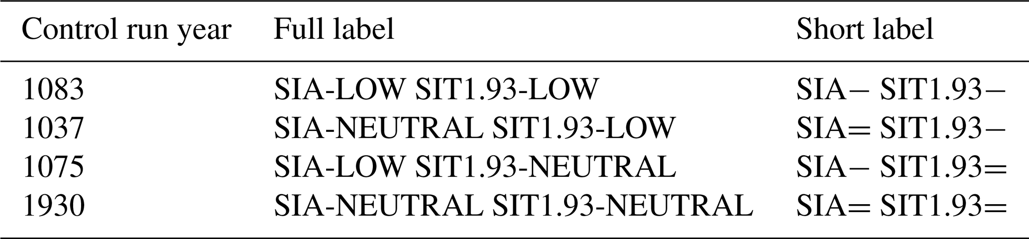
Within an individual ensemble, each trajectory starts from the same initial condition, as done for ensemble weather and seasonal climate predictions. In order to allow the trajectories to diverge from each other, we slightly perturb the surface pressure field of each trajectory as described in the Supplement of Ragone et al. (2018). The four different initial conditions for the four ensembles are sampled from the 3000-year control run according to different anomaly values of the January–February mean pan-Arctic sea ice area, i.e. the observable itself, and of the January–February mean cumulative area with sea ice thickness equal to or larger than 1.93 m (SIT1.93, Fig. 1 and Table 1). The choice of SIT1.93 is motivated by the studies of Chevallier and Salas-Mélia (2012) and Lindsay et al. (2008). According to those studies, the late-winter–early-spring cumulative area with sea ice thickness larger than a critical threshold has a larger impact on the late-summer sea ice area than the winter–spring sea ice volume and area itself. Here we apply a composite analysis to the PlaSim-LSG control run to identify a sea-ice-related variable whose anomaly value during the timing of the ensemble initialization has a potentially large connection with the probability of an extreme late-summer sea ice low (Fig. 1a; note that the critical thickness values of 0.2, 0.5, 0.66, 0.9, 1.5, 1.93, 2.5, 4, 4.2 and 6 m are selected from Chevallier and Salas-Mélia, 2012; Lindsay et al., 2008). Compared to the various variables shown in Fig. 1a, extremely negative February–September and August–September mean sea ice area anomalies are most strongly related to the January–February sea ice volume and cumulative area with sea ice thickness equal to or larger than a critical thickness between 1.8 and 2.1 m respectively. We choose SIT1.93 following the critical threshold used in Lindsay et al. (2008). We emphasize, however, that the labelling (“SIT1.93−”, “SIT1.93=”, “SIT1.93+”) of the selected initial conditions would be the same as in this study if the labelling were chosen according to the anomaly values of the cumulative area with sea ice thickness equal to or larger than the remaining thresholds between 1.80 and 2.10 m. In PlaSim-LSG, the correlations between SIT1.93 and the cumulative area with sea ice thickness equal to or larger than the remaining thresholds between 1.8 and 2.1 m are between 0.96 and 0.99, and the precise choice of a threshold between 1.8 and 2.1 m does not affect the interpretation of the results.

Table 1 The 6000-member control and 600-member rare event algorithm ensemble simulations running between 1 February and 30 September. Labelling of the experiments according to the different initial conditions with (middle column) the full label and (right column) short labels used in the text.

3 Results

Importance sampling of extreme sea ice lows and estimation of their probabilities

We exploit initialized ensemble simulations to investigate the statistical properties of extreme negative February–September and August–September mean pan-Arctic sea ice area anomalies as a function of four different initial winter sea ice states (see Sect. 2.2). The goal of using the rare event algorithm is to obtain a better statistics of extremely low sea ice area values than available from standard control ensemble simulations. Compared to the latter, the algorithm likewise allows the order of magnitude of a lower bound of sea ice area values that can be generated internally via atmosphere–ocean dynamics to be better inferred.

We show the time evolution of pan-Arctic sea ice area anomalies relative to the control ensemble mean and the distributions of summer sea ice area for the ensemble simulations starting from a neutral initial winter sea ice state (Fig. 2a, c, and e; control run model year 1930 and labelled as “SIA= SIT1.93=”; see Sect. 2.2 for more details) and from an initial winter state characterized by neutral sea ice area and extremely low cumulative area with sea ice thickness equal to or larger than 1.93 m (SIT1.93; Fig. 2b, d, and f; a control run model year 1037 and labelled as “SIA= SIT1.93−”; note that Fig. 2 compares for both initial conditions one realization of the rare event simulation with N=600 trajectories with the statistics of N=6000 control ensemble trajectories). Among all four experiments, the SIA= SIT1.93= and SIA= SIT1.93− rare event simulations delivers the trajectory with the most extremely negative August–September mean sea ice area anomaly relative to the corresponding control ensemble means (i.e. relative to the climatological mean values defined for the two sea ice initial conditions; these anomalies are in both cases $-\mathrm{1.87}\times {\mathrm{10}}^{\mathrm{6}}{\mathrm{km}}^{\mathrm{2}}$), and the SIA= SIT1.93− experiment produces the trajectory leading to the lowest August–September mean sea ice area value in an absolute sense among all available simulations.

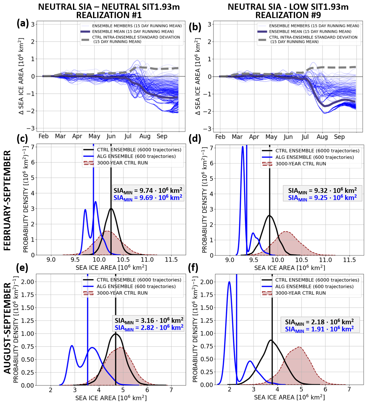
Figure 2 Ensemble simulations initialized on 1 February (a, c, e) 1930 and (b, d, f) 1037 of the control run. (a, b) Rare event simulations: N=600 trajectories (thin blue lines) and ensemble mean (thick blue line) of daily pan-Arctic sea ice area anomalies relative to the daily climatology of the corresponding control ensemble means. The dashed grey lines show the intra-ensemble standard deviations in the control ensembles. All lines are presented as 15 d running means. (c–f) Probability distribution functions of (c, d) February–September and (e, f) August–September mean pan-Arctic sea ice area for (blue) the rare event simulation, (black) the control ensembles (N=6000 trajectories) and (red) the 3000-year control run. The vertical lines show the mean of the distributions. The black and blue values indicate the smallest February–September and August–September mean sea ice area value in the control and rare event ensemble simulations respectively.

In both the SIA= SIT1.93= and SIA= SIT1.93− experiments, the differences between the sea ice area in the rare event algorithm and the control ensemble mean are small compared to the control intra-ensemble standard deviation until June (Fig. 2a and b). From the end of June onwards, trajectories generated with the rare event algorithm show a systematic shift towards lower sea ice area values compared to the control ensembles, reaching an ensemble mean shift of about $-\mathrm{1.2}\times {\mathrm{10}}^{\mathrm{6}}$ and $-\mathrm{1.5}\times {\mathrm{10}}^{\mathrm{6}}{\mathrm{km}}^{\mathrm{2}}$ in the SIA= SIT1.93= and SIA= SIT1.93− experiments respectively.

The biasing towards negative sea ice area anomalies with the rare event algorithm compared to the control ensemble reflects the importance sampling of extreme negative sea ice area anomaly values on average over the entire simulation period between February and September (Fig. 2c and d) (cf. Sauer et al., 2024a; Ragone and Bouchet, 2021). The distributions of February–September mean sea ice area obtained with the rare event algorithm fluctuate around a mean value in the lower tail of the control distribution, and their minimum sea ice area values are smaller than the minima obtained with the corresponding control ensembles (minimum February–September mean sea ice area values of 9.69×10⁶ and 9.25×10⁶ km² in the SIA= SIT1.93= and SIA= SIT1.93− rare event simulations vs. 9.74×10⁶ and 9.32×10⁶ km² in the corresponding control ensemble simulations). As the February–September mean sea ice area is strongly related to the August–September one (the minimum–maximum range of the correlation between both quantities across the members in all four control ensembles is [0.89 0.92]), the algorithm likewise improves the sampling efficiency of extremely low August–September mean sea ice area exceeding the lower range of sea ice area values obtained with the control ensembles (Fig. 2e and f); minimum August–September mean sea ice area values of 2.82×10⁶ and 1.91×10⁶ km² in the SIA= SIT1.93= and SIA= SIT1.93− rare event simulations vs. 3.16×10⁶ and 2.18×10⁶ km² in the control ensemble simulations). The distributions of sea ice area values obtained with the rare event algorithm show a bimodality in both experiments. We will address this behaviour in Sect. 5.

It is noticeable that the sea ice area obtained with the control and rare event ensemble simulations depends on the chosen initial condition (i.e. its location relative to the distribution of the 3000-year control run varies among the different experiments; Fig. 2c–f). In order to quantify the impact of the initial condition on extreme summer sea ice lows, we compare the probability of extreme negative February–September and August–September mean sea ice area anomalies between the four experiments (Fig. 3). We compute these probabilities as

$$\begin{array}{}\text{(4)}& {\displaystyle }{\displaystyle }P\left(a\right)={\displaystyle \frac{\mathrm{1}}{N}}\sum _{n=\mathrm{1}}^N{\mathbb{1}}_a\left(I_n\right)\text{ with }{\mathbb{1}}_a\left(I_n\right)=\left\{\begin{array}{ll}\mathrm{1},& I_n\le a\\ \mathrm{0},& I_n>a\end{array}\right.,\end{array}$$

where I_n is the February–September or August–September time-averaged pan-Arctic sea ice area in trajectory n,a is the amplitude of the sea ice area anomaly, N is the number of trajectories, and 𝟙_a(I_n) is the indicator function. As Eq. (4) represents the probability as an expectation value of the indicator function, probabilities from the simulations with the rare event algorithm can be computed by applying the estimator in Eq. (3) to this quantity (see Lestang et al., 2018; Ragone et al., 2018; Ragone and Bouchet, 2020; Sauer et al., 2024a).

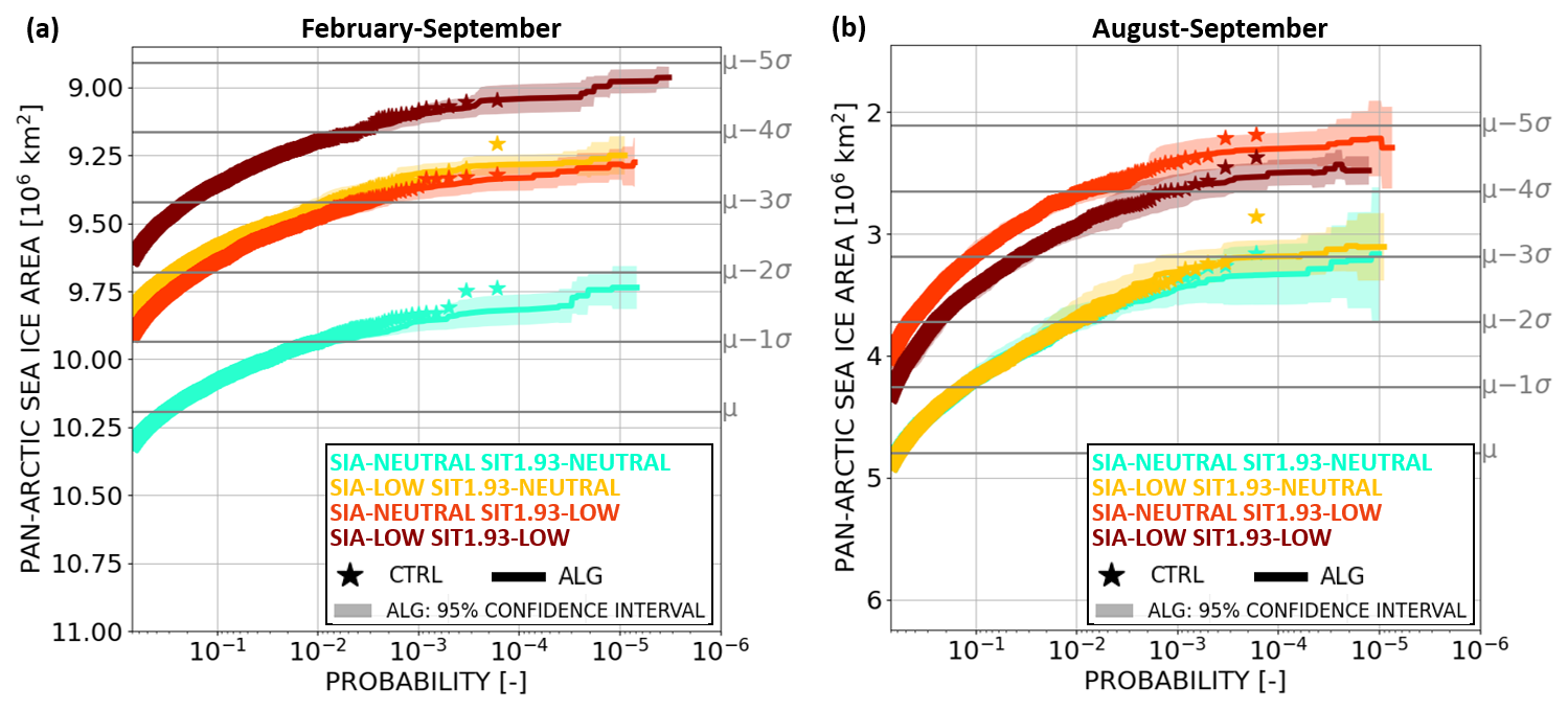
Figure 3 Probabilities (x axes) of (a) February–September and (b) August–September mean sea ice area equal to or smaller than a given threshold (y axes) as a function of four different initial conditions for (stars) the N=6000 trajectory control ensembles (i.e. 10 realizations are merged into one single ensemble) and (solid lines) the average over 4–10 algorithm estimates. The shading shows the 95 % confidence intervals derived from the t distribution of the 4–10 estimates (see Fig. S4 for a description of the computation of the confidence intervals). Note that the y axes are displayed in reverse order. In the legend, “SIA” and “SIT1.93” indicate the state of the January–February mean anomaly of the pan-Arctic sea ice area and the cumulative area with sea ice thickness equal to or larger than 1.93 m respectively. The grey labels on the right of each panel show how many standard deviations a sea ice area value is below the mean of the 3000-year control run.

In Fig. 3, the star markers show the probabilities estimated with the N=6000 trajectory control ensembles. The solid lines and the shading show the average estimates and 95 % confidence intervals obtained from multiple realizations of the rare event algorithm ensemble simulations respectively (see Fig. S4 for a description of the computation of the confidence intervals). The control and rare event algorithm estimates are consistent with each other where they overlap. Compared to the control ensembles, the major advantage of the algorithm is the access to much rarer events with the former than the latter, reaching probability values of 10⁻⁵ (0.001 %) for a computational cost of order 10³–10⁴ years. Moreover, compared to direct sampling, the rare event algorithm allows for a statistically more robust estimate of the probabilities of trajectories corresponding to the lower tail of the control distribution (i.e. corresponding to probability estimates below 10⁻³ in this application).

For a fixed probability level, the amplitudes of February–September and August–September mean sea ice area span a range of about 3 and 2 standard deviations among the different initial conditions. This confirms a strong impact of the initial condition on the amplitudes and probabilities of extreme negative summer sea ice area anomalies evaluated relative to the 3000-year control run baseline climatology (Fig. 3). Regarding the February–September seasonal average, a low state both in the winter SIT1.93 and in the winter sea ice area contribute to the preconditioning of an extreme (Fig. 3a). Consequently, the most extremely negative seasonally averaged sea ice area anomalies occur following years with a low winter state both in the sea ice area and in SIT1.93 (Fig. 3a). The contribution of low winter sea ice area and low SIT1.93 to these anomalies, however, is not fully additive (Fig. 3a). For a fixed probability level, the sum of the February–September mean sea ice area anomalies relative to the control run mean over the SIA= SIT1.93− and “SIA− SIT1.93=” experiments exceeds the sea ice area anomalies obtained with the “SIA− SIT1.93−” experiment in magnitude. We hypothesize that the preconditioning of low states of the seasonally mean sea ice area through low winter sea ice area and SIT1.93 is only efficient for a restricted geographic region where the climatological mean sea ice thickness is small enough to be able to form open water within one season. In parts of that region, the contribution of low winter sea ice area and SIT1.93 to an anomalously large area of open water during summer is likely to overlap spatially (i.e. open-water conditions prevail in certain grid boxes independent from whether both winter sea ice area and SIT1.93 are in a low state or only one of them). Moreover, the overlapping confidence intervals between the SIA= SIT1.93− and SIA− SIT1.93= experiments suggest that low winter states in the sea ice area and SIT1.93 are equally important in favouring an extremely negative February–September mean sea ice area anomaly.

Regarding the August–September mean, the contribution of a low winter sea ice area to an extreme is small compared to the contribution of a low winter state in SIT1.93 (Fig. 3b). Thus, similar amplitudes of extremely low August–September mean sea ice area occur for the SIA= SIT1.93= and SIA− SIT1.93= experiments. Likewise, the most extremely negative August–September mean sea ice area occurs in the experiment starting from an initial condition with a low SIT1.93 and a neutral winter sea ice area. A low winter sea ice area is therefore not required to produce the most extremely negative August–September sea ice area anomalies.

Despite the important role of preconditioning in favouring extremely low sea ice states, preconditioning represents only a necessary and not a sufficient condition for extremes with the largest amplitudes available in this study (Fig. 3 and Table 2). Extreme sea ice lows with sea ice area values corresponding to the 1 % percentile of the model distribution or less occur as a consequence of both winter sea ice–ocean preconditioning and anomalous intra-seasonal processes (e.g. weather patterns; see Sect. 4) that enhance sea ice reduction within one single melting season. The relative contribution of preconditioning to extreme sea ice lows vs. anomalous dynamics on an intra-seasonal timescale is larger for February–September than August–September mean sea ice area (Fig. 3 and Table 2). Thus, the February–September time-averaged control ensemble mean sea ice area anomaly for the SIA− SIT1.93−” initial condition explains about 65 % of the magnitude of the 1 % percentile of February–September mean sea ice area anomalies available from all the 10 SIA− SIT1.93− rare event algorithm ensemble simulations. In contrast, the August–September time-averaged control ensemble mean sea ice area anomaly for the experiments starting from a “SIT1.93−” initial condition is in magnitude on the order of 40 %–50 % of the 1 % percentile of August–September mean sea ice area anomalies available from 10 ensemble simulations with the rare event algorithm respectively (Fig. 3 and Table 2).

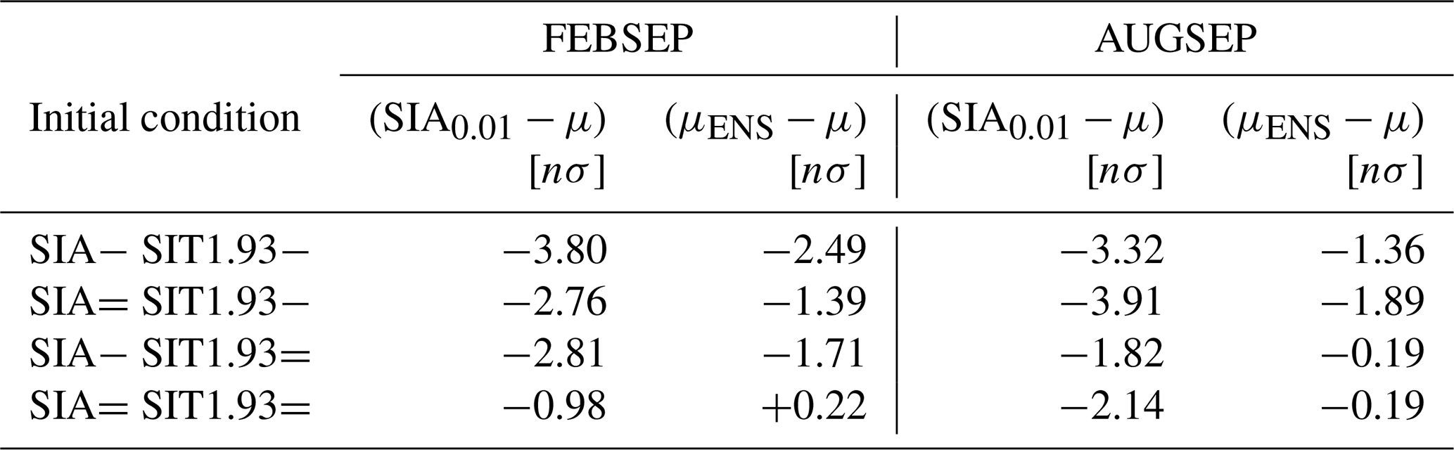
Table 2 February–September (FEBSEP) and August–September (AUGSEP) mean sea ice area anomalies relative to the mean μ of the 3000-year control run expressed in the unit of multiple control run standard deviations (“nσ” with n∈ℝ). “Control run” refers to a 3000-year-long integration of a single trajectory (presented in Sauer et al., 2024a), whereas “control ensembles” refer to multiple trajectories run from 1 February to 30 September and initialized from one single initial condition. The anomalies in the column “SIA_0.01−μ” correspond to the 1 % percentile sea ice area value (i.e. preconditioning + anomalous weather) presented as the average over 10 estimates available from the output of 10 rare event algorithm experiments. The anomalies in the μ_ENS−μ column correspond to the control ensemble mean, i.e. the impact of preconditioning on the mean of the N=6000 trajectory control ensemble. For the computation of the percentiles with the algorithm, we weight the contribution of each trajectory to the percentile by the product of Z_k and the exponential factor shown in Eq. (3).

The results obtained in Fig. 3 are consistent with the memory properties of the sea ice in the Arctic. Typically, late-summer sea ice area anomalies are poorly connected to the late-winter sea ice area (Blanchard-Wrigglesworth et al., 2011; Chevallier and Salas-Mélia, 2012; Day et al., 2014; Tietsche et al., 2014), explaining the non-existing contribution of winter sea ice area anomalies to extreme late-summer sea ice area lows. Compared to the sea ice area, quantities related to the sea ice thickness, as shown in Chevallier and Salas-Mélia (2012), act as a preconditioning for extreme reduction of sea ice area via its impact on the open-water formation efficiency during summer. The dependency of extreme negative seasonally averaged sea ice area anomalies on the winter sea ice area is explainable by the persistence of negative sea ice area anomalies from late winter to spring (Blanchard-Wrigglesworth et al., 2011).

4 Physical processes and conditions prior to sea ice lows with probabilities of less than 0.001 %

In this section we study the physical processes and conditions favouring extremely low late-summer sea ice area. In contrast to the work in Sauer et al. (2024a), the development of low sea ice states relative to the initial condition-specific control ensemble mean is entirely attributable to intra-seasonal drivers as all trajectories within an ensemble start from the same initial condition. Using the SIA= SIT1.93= and SIA= SIT1.93− experiments, we discuss the trajectory leading to the lowest August–September mean pan-Arctic sea ice area value available within each of the two experiments respectively (Figs. 4–7). The lowest August–September mean sea ice area values in the SIA= SIT1.93= and SIA= SIT1.93− ensembles are 2.82×10⁶ and 1.91×10⁶ km² and thus about 40 % and 49 % smaller than the control ensemble mean values of 4.69×10⁶ and 3.78×10⁶ km². These sea ice area anomalies are therefore larger in magnitude than the deviation of the observed 2012 mean August–September mean sea ice area from a trend line fitted to the period 1979–2006 (about −32 %; 3.09×10⁶ compared to 4.53×10⁶ km²; see Fig. S3 in the Supplement). The computation of the probabilities to generate a sea ice area equal to or smaller than a given threshold indicates that the sea ice lows in the trajectories of the two ensemble simulations are below 0.001 % (Fig. 3).

4.1 Seasonal evolution of the state of the sea ice

The most dominant negative sea ice area anomalies in both trajectories start to develop in June–July and reach their peak amplitudes in August–September (Fig. 4a and d). Negative August–September mean sea ice area anomalies are characterized by enhanced open-water area in the Barents and Kara seas, the eastern central Arctic Ocean, and the northern Canadian Archipelago (Fig. 4b and e). From late winter to late spring, sea ice area anomalies are close to zero in the SIA= SIT1.93= experiment. In the SIA= SIT1.93− experiment, sea ice area anomalies are slightly positive in early spring and are close to zero during late spring. The fact that winter–spring sea ice area anomalies are small in magnitude compared to the late-summer ones supports the conclusion from Fig. 3 that winter–spring sea ice area anomalies do not play an important role for the formation of late-summer sea ice lows.

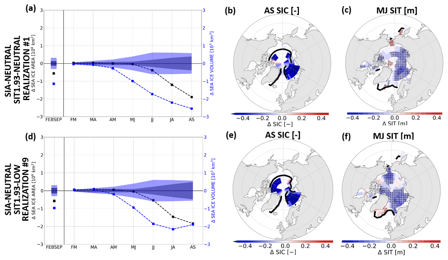
Figure 4 Trajectory with the lowest February–September and August–September mean pan-Arctic sea ice area obtained with the rare event simulation starting from a winter initial condition characterized by (a–c) neutral sea ice area and neutral SIT1.93 (control run year 1930) and (d–f) neutral sea ice area and low SIT1.93 (control run year 1037). (a, d) Pan-Arctic sea ice (black) area (10⁶ km²) and (blue) volume (10³ km³) anomalies. Shading shows the intra-ensemble standard deviation of the corresponding control ensemble. (b, e) August–September mean sea ice concentration and (c, f) May–June mean sea ice thickness anomalies. Hatching indicates anomalies larger in magnitude than the intra-ensemble standard deviation of the control ensemble. (a–f) All anomalies are computed with respect to the climatology of the corresponding control ensemble.

It is noticeable that late-summer negative sea ice area anomalies are preceded by negative pan-Arctic sea ice volume anomalies starting to develop in spring (Fig. 4a and d). These are related to the development of negative sea ice thickness anomalies before an anomalous reduction of the pan-Arctic sea ice area. In the SIA= SIT1.93= experiment, these negative sea ice thickness anomalies develop predominantly on the Eurasian side of the Arctic and northern of the Canadian Archipelago (Fig. 4c). In the SIA= SIT1.93− experiment, negative sea ice thickness anomalies are present from the Kara and Barents seas towards the Canadian Archipelago and in the Beaufort Sea. In both experiments, the anomalously strong sea ice thinning acts as a preconditioning for enhanced open-water formation in late summer as described in Chevallier and Salas-Mélia (2012). The presence of negative spring sea ice volume anomalies relative to the control ensemble mean suggests that the spring sea ice volume provides an additional source of predictability of extremely negative late-summer sea ice area anomalies relative to the climatology of the full control run on top of the predictability emerging from the late-winter initial condition. This result is consistent with the findings of Bonan et al. (2019) and Bushuk et al. (2020) according to which late-summer sea ice area is substantially stronger connected to late spring to early summer sea ice volume than to mid spring sea ice volume. In this way, sea ice volume contributes to a spring barrier of the predictability of late-summer sea ice area in addition to a part of the predictability barrier that may be purely related to a substantial increase in the persistence of sea ice area anomalies from May to July (Tietsche et al., 2014; Day et al., 2014; Bonan et al., 2019; Bushuk et al., 2020).

4.2 Seasonal evolution of the state of the atmosphere

We are interested in the processes favouring the development of negative sea ice thickness and ensuing negative sea ice area anomalies. Firstly, we analyse the seasonal evolution of 2 m temperature (T2M) and 500 hPa geopotential height (Z500) anomalies to establish a link between sea ice lows and the thermodynamic and dynamic states of the atmosphere (Fig. 5). The evolution of the atmospheric state differs between the SIA= SIT1.93= and SIA= SIT1.93− trajectories. In the SIA= SIT1.93= trajectory, the Arctic region is in an anomalously warm state from late winter to late spring. Positive T2M anomalies occur over the central Arctic Ocean in February–March and show a wavenumber-3-like positive T2M pattern in spring associated with a baroclinic signal in the 500 hPa geopotential height anomaly field (Fig. 5b, c, g, and h). In May–June, anomalously warm conditions prevail over the eastern Arctic and north of the Canadian Archipelago and thus spatially coincide with the region of negative sea ice thickness anomalies (cf. Figs. 5c and 4c). In June–July, the magnitude of T2M anomalies declines as 2 m temperatures are constrained by the climatological sea ice melting to be close to the freezing point (Fig. 5d). The re-emergence of anomalously warm conditions in August–September (Fig. 5e) may be both a driver of sea ice reduction and a consequence of reduced sea ice conditions. In contrast to the SIA= SIT1.93= experiment, February–March 2 m temperature anomalies in the SIA= SIT1.93− trajectory are close to zero over the Arctic Ocean (Fig. 5k). This approximately neutral temperature state is followed by a strong warming with a barotropic positive geopotential height anomaly response over the Norwegian Sea and the Arctic Ocean during spring (Fig. 5k, l, m, p, q and r). Positive 500 hPa geopotential height anomalies persist until early summer, while T2M values are constrained to be close to the freezing point in June–July in large parts of the Arctic Ocean before re-emerging in August–September as for the SIA= SIT1.93= trajectory (cf. Fig. 5n, o, s and t and d and e).

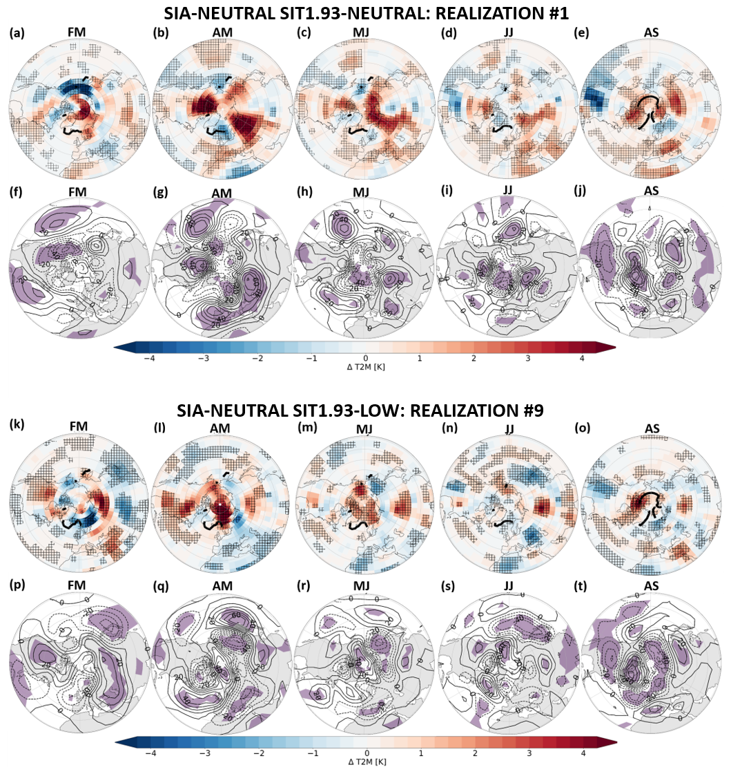
Figure 5 Trajectory with the lowest February–September and August–September mean pan-Arctic sea ice area in the rare event simulation starting from a winter initial condition characterized by (a–j) neutral sea ice area and neutral SIT1.93 (control run year 1930) and (k–t) neutral sea ice area and low SIT1.93 (control run year 1037). Panels (a)–(e) and (k)–(o) show February–March (FM), April–May (AM), May–June (MJ), June–July (JJ) and August–September (AS) mean T2M anomalies [K]. Panels (f)–(j) and (p)–(t) show FM, AM, MJ, JJ and AS mean Z500 anomalies [gpm]. Contour interval for Z500 is 10 gpm. Hatching indicates anomalies larger in magnitude than the intra-ensemble standard deviation of the control ensemble. All anomalies are computed with respect to the climatology of the corresponding control ensembles. The black contour line in (a)–(e) and (k)–(o) shows the climatological sea ice edge defined as the 15 % sea ice concentration contour line.

4.3 Surface energy budget analysis

We perform a surface energy budget analysis to understand how the anomalous reduction of sea ice is physically related to anomalous atmospheric conditions (Figs. 6 and 7). We define the surface energy budget for an infinitesimally thin interface without heat storage located between the atmosphere and the snow–sea ice–ocean system (cf. Serreze and Barry, 2014). The different terms of the budget are then given by

$$\begin{array}{}\text{(5)}& {\displaystyle }{\displaystyle }{R}_{\text{SW}}(\mathrm{1}-\mathit{\alpha })+R_{\text{LW}}+S+L=-\mathit{ϵ}\mathit{\sigma }{T}_{\mathrm{s}}^{\mathrm{4}}+Q+M,\end{array}$$

where R_SW and R_LW are the downward shortwave and downward longwave radiative fluxes respectively, α is the surface albedo, S and L are the sensible and latent heat fluxes, ϵ is the surface emissivity, $\mathit{\sigma }=\mathrm{5.67}\times {\mathrm{10}}^{-\mathrm{8}}\mathrm{W}{\mathrm{m}}^{-\mathrm{2}}{\mathrm{K}}^{-\mathrm{4}}$ is the Stefan–Boltzmann constant, and T_s is the surface temperature. Q summarizes conductive and turbulent energy fluxes between the surface and the snow–sea ice–ocean system. M is the energy flux associated with melting and freezing at the surface. Energy fluxes related to bottom sea ice growth, to temperature changes in the snow–sea ice–ocean system and to the vertical energy flux from the ocean into the sea ice are implicitly included in Q. In Fig. 6, we complement the analysis of the atmosphere–surface energy fluxes by the analysis of the vertical oceanic heat flux. If not stated otherwise, we define upward (downward) energy fluxes and associated flux anomalies to be positive (negative).

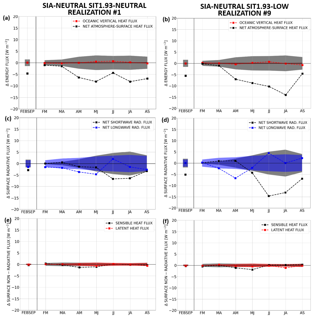
Figure 6 Trajectory with the lowest February–September and August–September mean pan-Arctic sea ice area in the rare event simulation starting from a winter initial condition characterized by (a, c, e) neutral sea ice area and neutral SIT1.93 (control run year 1930) and (b, d, f) neutral sea ice area and low SIT1.93 (control run year 1037). Mean energy flux anomalies [W m⁻²] on average over all ocean grid boxes northern of 70° N. (a, b) (black) Net atmosphere–surface energy flux (sensible + latent + net longwave + net shortwave) and (red) vertical ocean heat flux. (c, d) Net surface (blue) longwave radiative and (black) shortwave radiative flux. (e, f) Surface (red) latent and (black) sensible heat flux anomalies. The sign convention is chosen such that positive anomalies correspond to enhanced upward fluxes. (a–f) Shading indicates the intra-ensemble standard deviation of the corresponding control ensembles. All anomalies are computed with respect to the climatology of the corresponding control ensembles.

In both the SIA= SIT1.93= and SIA= SIT1.93− trajectories, strongly negative net surface-atmosphere energy flux anomalies occur over the Arctic Ocean from April–May to August–September, indicating an anomalous energy accumulation within the snow–sea ice–ocean system (Fig. 6a and b). Anomalies in the vertical oceanic heat flux are much smaller than the atmospheric ones but are still systematically positive in summer in both trajectories (Fig. 6a and b).

The contribution of different flux components to the negative net atmosphere–surface energy flux anomalies varies among the season, and both trajectories show two distinct phases. While these two phases show similarities between the two trajectories, their precise characteristics differ from each other. In the SIA= SIT1.93= trajectory, enhanced net energy accumulation in the snow–sea ice–ocean system during spring is predominantly explained by negative net longwave radiative flux anomalies and enhanced downward sensible heat fluxes (Fig. 6c and e). During summer, the anomalies in the atmosphere–surface energy transfer are dominated by the shortwave fluxes. Compared to the SIA= SIT1.93= trajectory, enhanced longwave radiative forcing on the sea ice in the SIA= SIT1.93− trajectory has a larger magnitude but is restricted to April–May (Fig. 6d). In May–June, instead, a transition takes place towards enhanced downward sensible heat fluxes and enhanced shortwave radiative forcing on the sea ice (Fig. 6d and f). The shortwave radiative forcing on the sea ice during middle to late summer is twice as large for the “SIA= SIT1.93=” trajectory as for the SIA= SIT1.93− trajectory.

We further subdivide the net shortwave and longwave radiative surface flux anomalies into their downward and upward components to trace back the net radiative surface flux anomalies to anomalous atmospheric conditions (Fig. 7). In the SIA= SIT1.93= trajectory, reduced downward solar radiation and enhanced downward longwave radiation occur in April–May and May–June (Fig. 7a and c). The signal in the longwave radiative fluxes is associated with enhanced atmospheric water vapour and cloudiness (Fig. 7e). In the SIA= SIT1.93− trajectory, instead, enhanced downward radiative flux anomalies associated with clouds and water vapour primarily occur in April–May (Fig. 7b, d, and f). In summer, a reduction in clouds occurs, and the shortwave radiative fluxes in combination with the sea ice–albedo feedback become the dominant driver of sea ice reduction in both experiments. The latter is, however, much more dominant in the SIA= SIT1.93− than in the SIA= SIT1.93= trajectory.

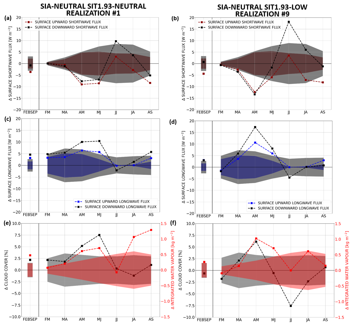
Figure 7 Trajectory with the lowest February–September and August–September mean pan-Arctic sea ice area in the rare event ensemble simulation starting from a winter initial condition characterized by (a, c, e) neutral sea ice area and neutral SIT1.93 (control run year 1930) and (b, d, f) neutral sea ice area and low SIT1.93 (control run year 1037). Mean anomalies of different quantities spatially averaged over all ocean grid boxes northern of 70° N. (a, b) Surface (dark red) upward and (black) downward shortwave radiative flux anomalies [W m⁻²]. (c, d) Surface (blue) upward and (black) downward longwave radiative flux anomalies [W m⁻²]. (a–d) Direction-independent absolute values of the downward and upward fluxes are considered; i.e. a positive (negative) anomaly indicates a radiative flux that is stronger (weaker) in magnitude than the climatology. (e, f) (black) Total cloud cover [%] and (red) integrated water vapour [kg m⁻²] anomalies. (a–f) Shading indicates the intra-ensemble standard deviation of the corresponding control ensembles. All anomalies are computed with respect to the climatology of the corresponding control ensembles.

5 Discussion and conclusions

We exploit four initialized ensemble simulations to study the statistical properties of extreme negative summer and late-summer pan-Arctic sea ice area anomalies as a function of four different initial winter states. Likewise, we investigate physical processes in two trajectories leading to extreme late-summer sea ice lows with larger amplitudes than the one observed in 2012. In order to circumvent the poor sampling of rare events in numerical simulations, we apply a rare event algorithm to improve the sampling efficiency of trajectories leading to extremely low pan-Arctic sea ice area on average over the melting season and during the annual sea ice minimum. The simulations with the rare event algorithm produce several hundreds of times more extremes than conventional control ensemble simulations for the same computational cost and allow extreme sea ice low probabilities to be estimated that are 2 orders of magnitude smaller compared to direct sampling (Fig. 3).

The approach used in this study is complementary to the rare event algorithm study of Sauer et al. (2024a). In their study, ensemble simulations are initialized with independent initial conditions sampled from an entire 3000-year control run, and the statistics computed with the rare event algorithm corresponds to unconditional probability distributions. Such an approach allows the sampling efficiency of low sea ice states to be improved, both related to multi-annual variability in the sea ice–ocean system (referred to as “preconditioning” in Sauer et al., 2024a) and driven by the dynamics occurring on intra-seasonal timescales. The single initial condition approach used in this study, instead, corresponds to a seasonal climate prediction set-up, giving access to the probability to observe an extreme late-summer sea ice low as a function of a given initial state. This approach also enables a targeted study of intra-seasonal drivers of anomalously strong sea ice reduction during the melting season. Within each ensemble simulation, a contribution of multi-annual sea ice–ocean preconditioning to the generation of low sea ice states compared to the control ensemble mean is by definition excluded as each trajectory starts from the same sea ice–ocean state.

The statistics obtained from the four different experiments indicates a strong impact of the late-winter sea ice initial condition on the probability and amplitudes of extremely negative summer pan-Arctic sea ice area anomalies computed relative to a 3000-year control run baseline climatology. For a fixed probability level, amplitudes of extremely negative February–September and August–September mean sea ice area anomalies span a range of about 3 and 2 control run standard deviations over the four experiments (Fig. 3 and Table 2). While winter preconditioning is a necessary condition to generate a sea ice low with an amplitude larger than a certain threshold, the most extreme sea ice lows available in this study require both preconditioning and anomalous intra-seasonal dynamics (e.g. anomalies in the atmospheric circulation) favouring enhanced reduction of sea ice area during the melting season (Fig. 3 and Table 2). The relative importance of preconditioning compared to intra-seasonal dynamics in driving extremely low sea ice area is larger for the February–September than August–September mean sea ice area (Table 2). Thus, about 65 % of the magnitude of the anomaly corresponding to the 1 % percentile value of February–September mean sea ice area in the “SIA− SIT1.93− experiment” is explainable by the impact of the preconditioning on the control ensemble mean sea ice area (Table 2). For August–September sea ice area, instead, about 40 %–50 % of the magnitude of the anomaly value corresponding to the 1 % percentile value is explainable by the impact of the preconditioning on the control ensemble mean in the experiments initialized with the SIA− SIT1.93− and SIA= SIT1.93− initial conditions (Table 2).

The analysis of the four initialized experiments suggests that an extremely negative February–September mean pan-Arctic sea ice area anomaly is preconditioned by low January–February mean states of both the pan-Arctic sea ice area and the cumulative area with sea ice thickness larger than a given threshold (the precise value used in this study is 1.93 m). In contrast, a source of predictability of an extreme late-summer sea ice low is given by the winter sea ice thickness information but not from the winter sea ice area. Both results are in line with the memory properties of the sea ice in the Arctic (Blanchard-Wrigglesworth et al., 2011; Chevallier and Salas-Mélia, 2012; Bonan et al., 2019; Bushuk et al., 2020; Tietsche et al., 2014). Using a preindustrial simulation with the Centre National de Recherches Météorologiques Coupled Global Climate Model version 3.3 (CNRM-CM3.3), Chevallier and Salas-Mélia (2012) find that the cumulative area with sea ice thickness larger than a threshold between 0.9 and 1.5 m provides a potential source of predictability of the September pan-Arctic sea ice area 6 months in advance. The authors argue that winter–spring sea ice thickness influences summer sea ice area by modulating the open-water-formation efficiency during the melting season. The dependency of extremely negative February–September mean sea ice area anomalies on both the winter SIT1.93 and winter pan-Arctic sea ice area itself can be explained by the fact that late-winter sea ice area anomalies have a non-zero persistence until spring (Blanchard-Wrigglesworth et al., 2011; Chevallier and Salas-Mélia, 2012). All in all, we emphasize that the precise critical sea ice thickness threshold used to define the cumulative area covered by sea ice thickness larger than a given value and the precise time lag may vary between different models.

Owing to the rare event algorithm, we analyse the physical properties in two individual trajectories leading to extremely negative August–September mean sea ice area anomalies with conditional probabilities of less than 0.001 %. While the precise thermodynamic and dynamical evolution of the atmosphere differs between both trajectories, common mechanisms can be detected between both trajectories. In both cases, an anomalously strong reduction of the pan-Arctic sea ice area in middle to late summer is anticipated by the development of negative sea ice thickness anomalies during spring. Even though this result is based on two individual trajectories instead of being inferred from a robust statistics of extreme sea ice low events, it suggests that late spring to early summer sea ice volume potentially provides an additional source of predictability of extremely negative late-summer sea ice area anomalies relative to the full control run in addition to the predictability associated with the late-winter initial condition. This finding is consistent with the studies of Bonan et al. (2019) and Bushuk et al. (2020). Bonan et al. (2019) and Bushuk et al. (2020) argue that sea ice volume captures a spring barrier in the predictability of late-summer sea ice area, resulting from the fact that late-summer sea ice area is substantially stronger connected to late spring to early summer sea ice volume than to the sea ice volume during mid spring. Apart from a small contribution of enhanced vertical ocean heat flux anomalies to the anomalous reduction of sea ice in the two trajectories discussed in this study, the largest amount of net energy accumulation in the sea ice–ocean system is related to enhanced downward net atmosphere–surface energy fluxes. Within the season, we observe two phases with two different physical properties. During spring, enhanced cloudiness and atmospheric water vapour results in negative (i.e. downward) net surface longwave radiative flux anomalies, providing enhanced energy to warm or melt sea ice. This is consistent with the finding of Kapsch et al. (2013, 2019), showing that observed extreme September sea ice lows have been preceded by enhanced downward longwave radiative fluxes in an anomalously moist and cloudy atmosphere. During summer, anomalous reduction of sea ice area is favoured by enhanced downward solar radiative flux, the sea ice–albedo feedback and enhanced open-water-formation efficiency in an anomalously thin sea ice environment.

We hypothesize that the bimodality in the distribution of late-summer sea ice area values obtained with the rare event simulation (Fig. 2) is favoured by the particular characteristics of the atmosphere–sea ice–ocean system in the Arctic, including preconditioning of anomalously low sea ice area via enhanced spring sea ice thinning and amplifying feedback mechanisms. A bimodality in a rare event simulation, however, does not necessarily imply a physical bimodality in the real model distribution. It could also be purely related to sampling (Ragone and Bouchet, 2021). For example, the peak of the probability density function at an August–September mean sea ice area value of 2.9×10⁶ km² in the “SIA= SIA=” experiment is related to hundreds of replicated trajectories originating from two ancestors (cf. Figs. 2a and e and S4). The bimodality may therefore simply emerge from the fact that trajectories leading to sea ice area values corresponding to the local minimum of the probability density function are undersampled in this particular simulation. Out of the 10 realizations of the “SIA= SIA=” experiment, a pronounced bimodality as in Fig. 2e occurs in a total number of three realizations (cf. Figs. 2a, c, and e and S5 in the Supplement). The August–September mean sea ice area values at which the two peaks and the local minimum of the probability distribution functions occur, however, vary from one realization to the next (cf. Figs. 2e and S5). Therefore, we do not expect that the real model probability density function has a bimodality explained by two peaks at specific sea ice area values. Nevertheless, we point out that trajectories belonging to the peak at August–September mean sea ice area values of 2.9×10⁶ km² show different physical characteristics to the ones leading to sea ice area values centred around a peak at 3.75×10⁶ km² (cf. Fig. 2e and Figs. S4 and S6 in the Supplement). Thus, compared to the latter, the former show a more pronounced spring preconditioning via anomalously strong sea ice thinning in a more humid Arctic atmosphere and a more pronounced water vapour feedback during late-summer (Fig. S6).

This study shows how rare event algorithms can be applied to initialized ensembles to study the probability of extreme states conditional on given initial conditions. This approach could be extremely useful in the context of seasonal to decadal predictions, in terms of both risk quantification and informing of the ensemble initialization strategies by the identification of important physical drivers for the development of extremes. The approach can be used to better quantify the relative contribution of a given initial condition to specific extreme sea ice loss events such as observed as in 2007 and 2012 (by comparing an ensemble initialized with the state of, for example, 1 March 2012 of a historical simulation with an ensemble initialized with the state of, for example, 1 March 1979 of a historical simulation). Moreover, the experimental design can be adapted to make quantitative statements about the relative contributions of global warming vs. internal climate variability to the probabilities and amplitudes of extreme sea ice loss events and to quantify the probability of observing a sea-ice-free Arctic within a given period of time. This can be achieved by initializing an ensemble with late-winter initial conditions sampled from, for example, the period 2016–2025 (i.e. an ensemble of 300 trajectories could be generated by producing 30 perturbed replicates of one initial condition per year respectively) and comparing the statistics with another ensemble initialized with data drawn from, for example, the period 1986–1995 of a historical simulation. In this study, we use the rare event algorithm to provide an estimate of the probability of a 2012-like late-summer sea ice area anomaly relative to a linear trend fitted to the period 1979–2006 (see Fig. S3). As described in Sect. 4, the observed August–September mean sea ice area anomaly in 2012 deviated by $-\mathrm{1.44}\times {\mathrm{10}}^{\mathrm{6}}{\mathrm{km}}^{\mathrm{2}}$ from that trend line. The probabilities of generating a sea ice area anomaly being equal to or larger than $-\mathrm{1.44}\times {\mathrm{10}}^{\mathrm{6}}{\mathrm{km}}^{\mathrm{2}}$ in magnitude compared to the control ensemble mean (i.e. related to processes on an intra-seasonal timescale) estimated with the four PlaSim ensemble simulation experiments range between $\mathrm{2.99}\times {\mathrm{10}}^{-\mathrm{5}}$ and $\mathrm{7.59}\times {\mathrm{10}}^{-\mathrm{4}}$ (Fig. 3).

Finally, we emphasize that this study is based on a relatively low resolution climate model with a purely thermodynamic sea ice model. A variety of idealizations such as the lack of sea ice dynamics (Wang et al., 2009; Ogi et al., 2016), the coarse atmospheric and oceanic resolutions (Docquier et al., 2019), biases in the mean sea ice thickness state (cf. Fig. S2b and p. 207 of Chevallier et al., 2019), response of clouds to sea ice changes, and the binary sea ice concentrations without representation of polynyas potentially affect the results about the physical drivers and the estimation of the probabilities of low sea ice states. Due to the lack of sea ice dynamics, the impact of anomalous winds associated with anomalous states of the Arctic Oscillation (AO) and the Arctic Dipole Anomaly (ADA) pattern on the export of sea ice from the marginal Arctic seas into the central Arctic Ocean and out of the Arctic via Fram Strait (Wang et al., 2009; Ogi et al., 2016), as well as the dynamical impact of synoptic storms on the sea ice (Zhang et al., 2013), is not captured in this model. We hypothesize that this leads to an underestimation of the amplitude of the most extremely negative sea ice area anomalies compared to more complex models than PlaSim. Consequently, the lack of sea ice dynamics potentially also leads to an underestimation of the probability of observing a 2012-like sea ice area anomaly presented in this study. Moreover, regional biases in the sea ice thickness field in PlaSim-T21-LSG compared to the PIOMAS reanalysis (sea ice too thick on annual average around the North Pole and in the Barents Sea; cf. Fig. S2b and p. 207 of Chevallier et al., 2019) may affect the results of this study. Thus, the trajectories with the most extremely negative sea ice concentration anomalies available from the ensembles show no substantial sea ice concentration anomalies around the North Pole, while strongly negative sea ice concentration anomalies are present in the Barents and Kara seas (Fig. 4). In observations, the Barents and Kara seas are sea-ice-free in late summer (Kapsch et al., 2019). While the overestimation of sea ice in the Barents and Kara seas in PlaSim compared to observations likely contributes to an overestimation of the amplitudes of extremely negative pan-Arctic sea ice area anomalies compared to the real world, an opposing effect is to be expected from the positive sea ice thickness bias around the North Pole in PlaSim compared to observations.

All in all, based on the analysis of two individual trajectories, the present study illustrates possible thermodynamics states of the atmosphere to generate sea ice lows larger in magnitude than the one observed in 2012. Likewise, it makes an important step forward towards the computation of probabilities of extreme Arctic sea ice lows as a function of different initial and climate states. A similar rare event algorithm study using the EC-Earth model version 3.3.1, including a more complex physics than PlaSim and a dynamic sea ice model, initialized with two sea ice–ocean initial conditions selected from a historical run, is in preparation. A possibility to rely on multiple models instead of one single model will consist in complementing the EC-Earth3 study by an analysis of extreme sea ice lows in existing large ensembles of the models of the Phases 5 and 6 of the Coupled Model Intercomparison Project.