The effect of noise on the stability of convection in a conceptual model of the North Atlantic subpolar gyre

The North Atlantic subpolar gyre (SPG) plays a fundamental role in the Atlantic ocean circulation by providing an important connection between the subtropical Atlantic and the Arctic. It is driven by both wind and density differences that are, in part, caused by convection in the Labrador Sea. Through this deep convection site, the SPG is also linked to the AMOC. There is considerable evidence that this area of convection may diminish or shift in a changing climate. For this reason, the convection in the SPG is considered a tipping point. Here, we extensively study a conceptual model of the SPG to characterize the stability of convection in the gyre. The bifurcation structure of this model is analyzed in order to identify bistable parameter regions. For a range of gyre salinity and freshwater forcing levels the gyre is found to have both convective and non-convective states. Furthermore, noise-induced transitions between convective and non-convective states are possible for a wide range of parameter values. Convection in the SPG becomes increasingly unstable as the gyre salinity decreases and the freshwater forcing increases. However, convection never fully stops and can always restart after a period of no convection. This indicates that, at least in this conceptual model, a collapse of convection in the SPG does not have to be permanent.

1 Introduction

The North Atlantic subpolar gyre is a cyclonic ocean circulation that includes parts of the North Atlantic Current, the Irminger current and Labrador current (Li and Born, 2019). As such, it provides a connection between the subtropical Atlantic and the Arctic. The horizontal circulation in the gyre dominates heat and salt transport in the subpolar latitudes of the Atlantic (Born and Stocker, 2014; Klockmann et al., 2020). It is also connected to deep convection sites in the Labrador, Irminger and Iceland basins (e.g. Lozier et al., 2019). Due to these characteristics and its position, the area has been described as “a key coupling region where vigorous wind systems encounter the southernmost extensions of sea ice and the most variable currents of the North-Atlantic with connections to the deep ocean via convection” (Li and Born, 2019).

The SPG is also connected to the Atlantic Meriodional Overturning Circulation (AMOC, e.g. Spooner et al., 2020) through its link to deep water formation sites in the Labrador Sea, Nordic Seas, and Irminger and Iceland basins. Conceptual modelling studies have indicated that the collapse of convection in the Labrador Sea could precede a collapse of the AMOC (Neff et al., 2023). The exact nature of the coupling between the AMOC and the SPG is up to some debate, but there is agreement on the fact that the SPG and AMOC are coupled and that their interactions can lead to abrupt climate transitions such as Dansgaard-Oescher events, during which temperatures at high latitudes in the Atlantic suddenly increase (Li and Born, 2019; Prange et al., 2023; Klockmann et al., 2020).

For the reasons listed above, variability in SPG circulation and convection strength is of considerable interest. Model simulations by Born and Mignot (2012) have shown that the SPG circulation is variable with a period of 15–20 years. They suggested that these internal variations are caused by an advection-convection feedback. In this feedback, a strong gyre circulation advects salt out of the SPG's center on short timescales, but on longer timescales the strong circulation leads to an increase of salinity due to lateral advection by eddies. An increase in salinity facilitates deep convection which in turn strenghtens the gyre circulation. This combination of a negative feedback on short timescales and a positive one on longer timescales provides the basis for SPG variability. In addition to this advection-convection feedback, SPG behavior has also been to shown to be affected by sea ice cover due to the gyre's sensitivity to buoyancy and wind forcings on longer timescales (Steinsland et al., 2023)

Besides varying in strength, convection in the subpolar gyre has been observed to shut down altogether, most recently in 2023 (Yashayev, 2024). These shutdowns are often associated with so-called Great Salinity Anomalies (GSAs). First documented in the late 1970s and early 1980s (Lazier, 1980; Dickson et al., 1988) and observed again in the late 1980s (Belkin et al., 1998) and 2010s (Biló et al., 2022), during these events watermasses of relatively low salinity are advected throughout the Northern seas, sharply decreasing the sea surface salinity in the region. These fresh water masses have been linked to anomalous sea ice melt in the high Arctic and Nordic seas (Yashayev, 2024; Allan and Allan, 2024). Convection in the Labrador sea can be inhibited temporarily by the passage of GSAs, although anomalous atmospheric conditions and the North Atlantic Oscillation state have also been identified as major forcing mechanisms that can both stop and restart convection (e.g. Gelderloos et al., 2012; Kim et al., 2021; Yashayev, 2024). These observations are in agreement with theoretical results that show, based on the geometry of the basin and a typical atmospheric forcing, that the Labrador sea is not far from a state that cannot support deep convection (Spall, 2012).

Despite its high variability and importance in linking various elements of the climate system, it is uncertain how the convection in the SPG will respond to climate change. Sgubin et al. (2017) showed that in CMIP5, the subpolar gyre region can experience sudden cooling during the 21st century and subsequent reduced temperatures until the end of the simulation. In most models this cooling is caused by a permanent collapse of convection in the SPG. Such an abrupt cooling occurred in 45.5 % of the subset of best performing models in the CMIP5 ensemble, and in 36.4 % of the best performing models in CMIP6 (Swingedouw et al., 2021). In addition, analysis of the CESM Large Ensemble has shown that shutdown of deep convection in the North Atlantic can be stochastically triggered, making it hard to predict when this shutdown could occur (Gu et al., 2024). The importance of stochastic atmospheric forcing on triggering instabilities was also noted by Swingedouw et al. (2021).

On the other side of the model spectrum, conceptual models have been used to study the stability of convection and circulation in the North Atlantic subpolar gyre. Most notably, Born and Stocker (2014) formulated a four box model for the convective basin of the Labrador sea. This model builds on Welander (1982), Rahmstorf (2001) and Kuhlbrodt et al. (2001)'s previous conceptual models of convection and extends models of the gyre and circulation in marginal seas by Spall (2004), Straneo (2006), Deshayes et al. (2009) and Spall (2012). In this, a hysteresis in gyre strength for variations in both the gyre current's salinity and freshwater forcing was found. These hystereses are caused by the formation of a strong baroclinic flow when the density difference between the inside and outside of the gyre is sufficiently high. Although this model is heavily simplified, when it is forced with reanalyzed surface temperatures the model mostly reproduces the observed gyre strenghts (Born et al., 2015), giving the model credibility.

Models of various complexity indicate that it remains elusive whether the North Atlantic subpolar gyre will continue to support convection in a changing climate. The collapse of convection in the SPG has been recognized as a potential tipping point in the climate system (Loriani et al., 2025). The critical value of global surface temperature associated with this tipping point is estimated to be 1.1 to 3.8 °C of global warming, and changes could occur with a relatively rapid timescale of approximately 10 years (Armstrong McKay et al., 2022). Such a collapse could potentially strongly influence surface temperatures and other climatic variables in the Atlantic and Nordic seas, as well as shifting the atmospheric jet stream (Swingedouw et al., 2021; Loriani et al., 2025). The SPG's connection to the AMOC is worrisome, as conceptual modelling studies have shown that a freshwater-driven collapse of convection in the gyre could influence the stability of the AMOC (Neff et al., 2023). There are also indications that a collapse of convection in the SPG can precede an AMOC collapse (Danabasoglu et al., 2016; Drijfhout et al., 2025). Lastly, external changes to the gyre system such as an increase in Greenland Ice Sheet runoff would serve to decrease the gyre current's salinity and therefore influence the SPG's stability. In fact, observations indicate that the North Atlantic, and the Irminger current in particular, are freshening (de Steur et al., 2018; Fried et al., 2024). It is likely that these changes will have an influence on the SPG's stability.

In this paper, we investigate the stability of convection in the North Atlantic subpolar gyre using an adjusted version of the simple conceptual model of the SPG that was initially introduced by Born and Stocker (2014, herafter referred to as BS14). We analyze the bifurcation structure of the model and subsequently apply noise to its salinity budget, in order to investigate if this noise can induce transitions to a state without convection. Section 2 provides a detailed description of the stochastic model and outlines the methods used. In Sect. 3.1 the bifurcation structure of the model without noise is presented, and various dynamical regimes of this deterministic model are identified in Sect. 3.2. We then study the dynamics of the model when noise is applied in Sect. 3.3 and 3.4. The results and some limitations of the model are discussed in Sect. 4.

2 Model and methods

2.1 Model formulation

In this section we present a box model of the SPG. It consists of a center part where convection takes place and a gyre circulation around that center. It is derived from BS14 and in Fig. 1 a diagram of the model is shown. At the center of the model are two vertically stacked cylindrical boxes (box 1, 3), representing the convective basin. These boxes are both surrounded by an annular box (box 2, 4) which represent the surface and deep gyre currents (U_s and U_d, respectively) around the center. The ratio of the height of the surface and deep box is denoted by r. There are no currents in the inner boxes and convective mixing can only take place between the inner boxes. The four boxes have the following properties:

• Box 1 is the cylindrical inner box at the air-water interface, with temperature T₁ and salinity S₁. It is the only one of the four boxes in which atmosphere-ocean interactions take place. It is exposed to an atmosphere with temperature T₀. An external freshwater flux (denoted by F) enters through the surface. Physically, this freshwater flux consists mostly of precipitation. There is an eddy heat and salt flux (E) between box 1 and 2, and convective mixing (C) between box 1 and 3 can occur.

• Box 2 is the annular outer box with temperature T₂ and salinity S₂. The surface gyre current flows in this box. Variations in salinity, such as Great Salinity Anomalies, are transported by the gyre current in this box of the model. The upper boundary current is denoted by U_s.

• Box 3 is the deep cylindrical inner box, with temperature T₃ and salinity S₃. There is an eddy heat and salt flux (E) between box 3 and 4, and convective mixing (C) between box 3 and box 1 can occur.

• Box 4 is the annular outer box with temperature T₄ and salinity S₄. The deep gyre current flows in this box. The lower boundary current is denoted by U_d.

It should be noted here that the temperature and salinity of boxes 2 and 4 are not explicitly modelled, but merely act as boundary conditions for the dynamic processes in boxes 1 and 3.

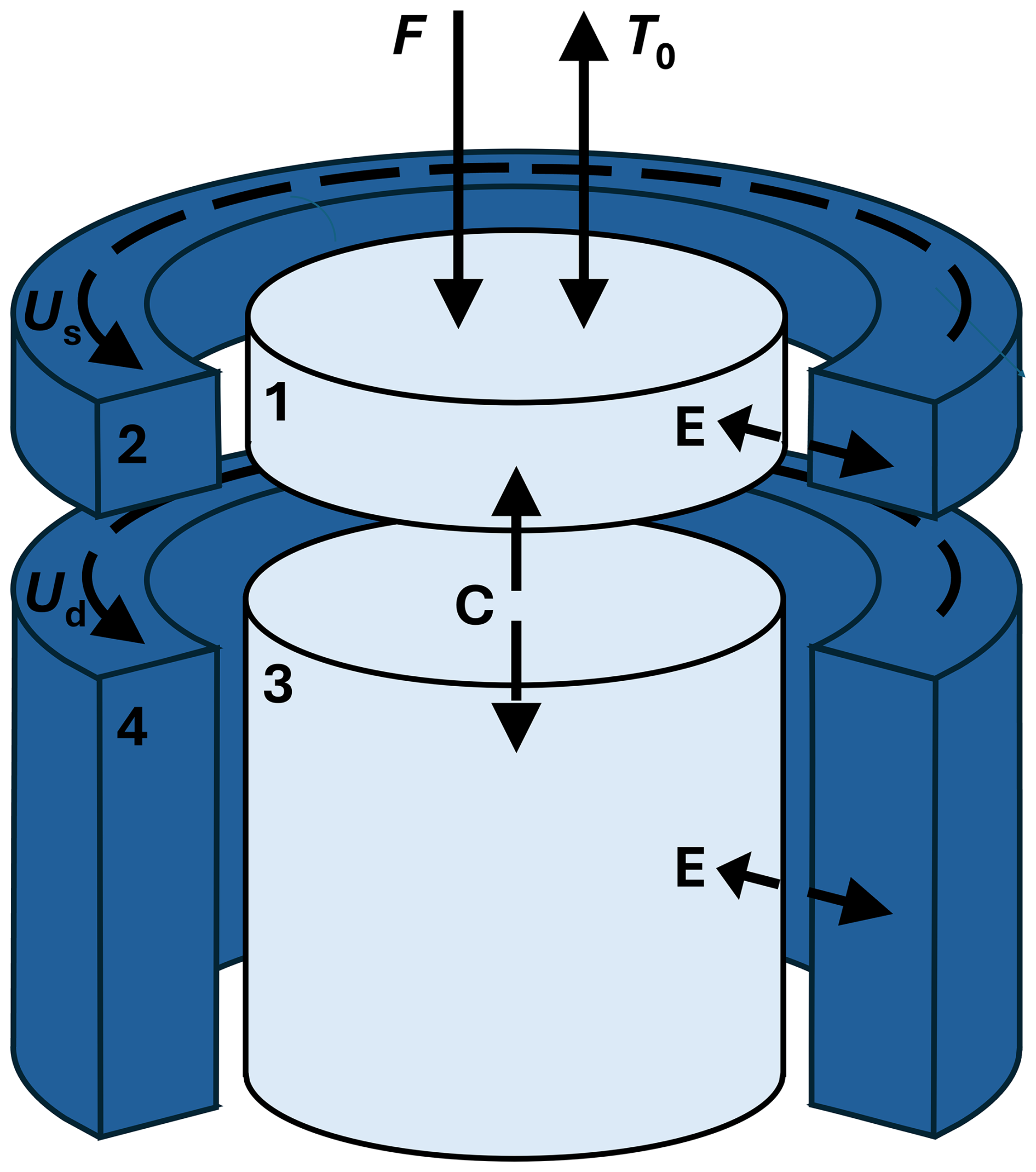
Figure 1 Illustration of the four-box model. Numbers 1 to 4 denote the boxes, U_s and U_d the surface and deep gyre current, F the surface freshwater forcing and T₀ the atmospheric temperature. Transport between the horizontal boxes can occur as eddy fluxes (E). Convection (C) can occur between boxes 1 and 3. Figure adapted from BS14.

In order to perform a bifurcation analysis, we adjusted BSl4 by non-dimensionalizing it and parameterizing convection continously. In addition, the model was made autonomous by considering a constant, rather than a seasonally varying, atmospheric temperature T₀. Lastly, we modelled the effect of noise in the salinity budget by adding additive noise terms in the differential equations that describe the surface box salinity S₁ and the surface velocity U_s. These noise terms represent stochastic variations in the surface current's salinity S₂ and the freshwater flux F and are therefore directly applied to S₂ and F, rather than to the boxes. Details on the derivation of this model and its relation to the original model can be found in Appendix A.

The adjusted, stochastic model is outlined in Eq. (1):

$$\begin{array}{ll}\text{(1a)}& {\displaystyle }{U}_{\mathrm{d}}& {\displaystyle }=U_{\mathrm{btp}}-\mathit{\eta }\left[\right(S_{\mathrm{4}}-T_{\mathrm{4}})-(S_{\mathrm{3}}-T_{\mathrm{3}}\left)\right],{\displaystyle }{U}_{\mathrm{s}}& {\displaystyle }=U_{\mathrm{btp}}-\mathit{\eta }\left[\right(S_{\mathrm{4}}-T_{\mathrm{4}})-(S_{\mathrm{3}}-T_{\mathrm{3}}\left)\right]\\ \text{(1b)}& {\displaystyle }& {\displaystyle }-\mathit{\eta }r\left[\right(S_{\mathrm{2}}+{\mathit{\zeta }}_S-T_{\mathrm{2}})-(S_{\mathrm{1}}-T_{\mathrm{1}}\left)\right],{\displaystyle \frac{\mathrm{d}{T}_{\mathrm{1}}}{\mathrm{d}t}}& {\displaystyle }={\mathit{\mu }}_{\mathrm{H}}{U}_{\mathrm{s}}(T_{\mathrm{2}}-T_{\mathrm{1}})+{\mathit{\mu }}_{\mathrm{C}}(T_{\mathrm{3}}-T_{\mathrm{1}})\mathcal{H}\left(\right(S_{\mathrm{1}}-T_{\mathrm{1}})\\ \text{(1c)}& {\displaystyle }& {\displaystyle }-(S_{\mathrm{3}}-T_{\mathrm{3}}))+{\mathit{\mu }}_{\mathrm{A}}(T_{\mathrm{0}}-T_{\mathrm{1}}),{\displaystyle \frac{\mathrm{d}{S}_{\mathrm{1}}}{\mathrm{d}t}}& {\displaystyle }={\mathit{\mu }}_{\mathrm{H}}{U}_{\mathrm{s}}(S_{\mathrm{2}}+{\mathit{\zeta }}_S-S_{\mathrm{1}})\\ {\displaystyle }& {\displaystyle }+{\mathit{\mu }}_{\mathrm{C}}(S_{\mathrm{3}}-S_{\mathrm{1}})\mathcal{H}\left(\right(S_{\mathrm{1}}-T_{\mathrm{1}})-(S_{\mathrm{3}}-T_{\mathrm{3}}\left)\right)\\ \text{(1d)}& {\displaystyle }& {\displaystyle }-(F+{\mathit{\zeta }}_F),{\displaystyle \frac{\mathrm{d}{T}_{\mathrm{3}}}{\mathrm{d}t}}& {\displaystyle }={\mathit{\mu }}_{\mathrm{H}}{U}_{\mathrm{d}}(T_{\mathrm{4}}-T_{\mathrm{3}})-{\mathit{\mu }}_{\mathrm{C}}r(T_{\mathrm{3}}-T_{\mathrm{1}})\mathcal{H}\left(\right(S_{\mathrm{1}}-T_{\mathrm{1}})\\ \text{(1e)}& {\displaystyle }& {\displaystyle }-(S_{\mathrm{3}}-T_{\mathrm{3}})),{\displaystyle \frac{\mathrm{d}{S}_{\mathrm{3}}}{\mathrm{d}t}}& {\displaystyle }={\mathit{\mu }}_{\mathrm{H}}{U}_{\mathrm{d}}(S_{\mathrm{4}}-S_{\mathrm{3}})-{\mathit{\mu }}_{\mathrm{C}}r(S_{\mathrm{3}}-S_{\mathrm{1}})\mathcal{H}\left(\right(S_{\mathrm{1}}-T_{\mathrm{1}})\\ \text{(1f)}& {\displaystyle }& {\displaystyle }-(S_{\mathrm{3}}-T_{\mathrm{3}})),\text{(1g)}& {\displaystyle \frac{\mathrm{d}{\mathit{\zeta }}_S}{\mathrm{d}t}}& {\displaystyle }=-{\displaystyle \frac{{\mathit{\zeta }}_S}{{\mathit{\tau }}_S}}+{\mathit{\sigma }}_S\mathit{\xi },\text{(1h)}& {\displaystyle \frac{\mathrm{d}{\mathit{\zeta }}_F}{\mathrm{d}t}}& {\displaystyle }=-{\displaystyle \frac{{\mathit{\zeta }}_F}{{\mathit{\tau }}_F}}+{\mathit{\sigma }}_F\mathit{\xi },\end{array}$$

where S_i and T_i (for $i=\mathrm{1},\mathrm{\dots },\mathrm{4}$) denote the salinity and temperature of the boxes as outlined above, the term S_i−T_i is a nondimensional expression for the density in box i, U_btp is the barotropic component of the boundary current with a constant strength of 20 Sv, r represents the ratio of the surface and deep box height, η determines the strength of the thermal wind, μ_H is the efficiency of horizontal mixing, μ_C is the efficiency of convection, and μ_A is the efficiency of atmosphere-ocean exchange. An overview of these parameters with their values and physical interpretations can be found in Table 1. The terms ζ_S and ζ_F are the stochastic components of this model, which are described by Ornstein-Uhlenbeck processes (e.g. Penland and Ewald, 2008; Boers et al., 2022; Ditlevsen and Johnsen, 2010). The evolution of these terms is described by their own differential equations (Eq. 1g and h). They consist of a noise term σ_Xξ, where ${\mathit{\sigma }}_X^{\mathrm{2}}$ is the variance of the noise and ξ represents a white noise process. In addition, the processes have a relexation timescale τ_X. The addition of this timescale ensures that the noise is correlated in time and not completely re-initialized at every timestep. The deterministic version of the model, which is discussed in Sect. 3.1 and 3.2, is a special case of Eq. (1) with ζ_S, σ_S, ζ_F and σ_F set to zero.

The function ℋ(x) in Eq. (1) is the step-like function

$$\begin{array}{}\text{(2)}& \mathcal{H}\left(x\right)={\displaystyle \frac{\mathrm{1}}{\mathrm{2}}}+{\displaystyle \frac{\mathrm{1}}{\mathrm{2}}}\tanh \left(kx\right)\end{array}$$

with k≫1. We introduce a step function to make the model continous. This choice is elaborated on in Appendix A.

Lastly, the dimensionless horizontal volume transport of the gyre is defined as

$$\begin{array}{}\text{(3)}& M=r{U}_{\text{s}}+U_{\text{d}}.\end{array}$$

The model (Eq. 1) consists of two velocity terms and six differential equations: four describing the evolution of the prognostic variables $T_{\mathrm{1}},S_{\mathrm{1}},T_{\mathrm{3}},S_{\mathrm{3}}$, and two describing the evolution of the noise terms ζ_S and ζ_F. All other parameters, including $T_{\mathrm{2}},S_{\mathrm{2}},T_{\mathrm{4}}$ and S₄, are prescribed.

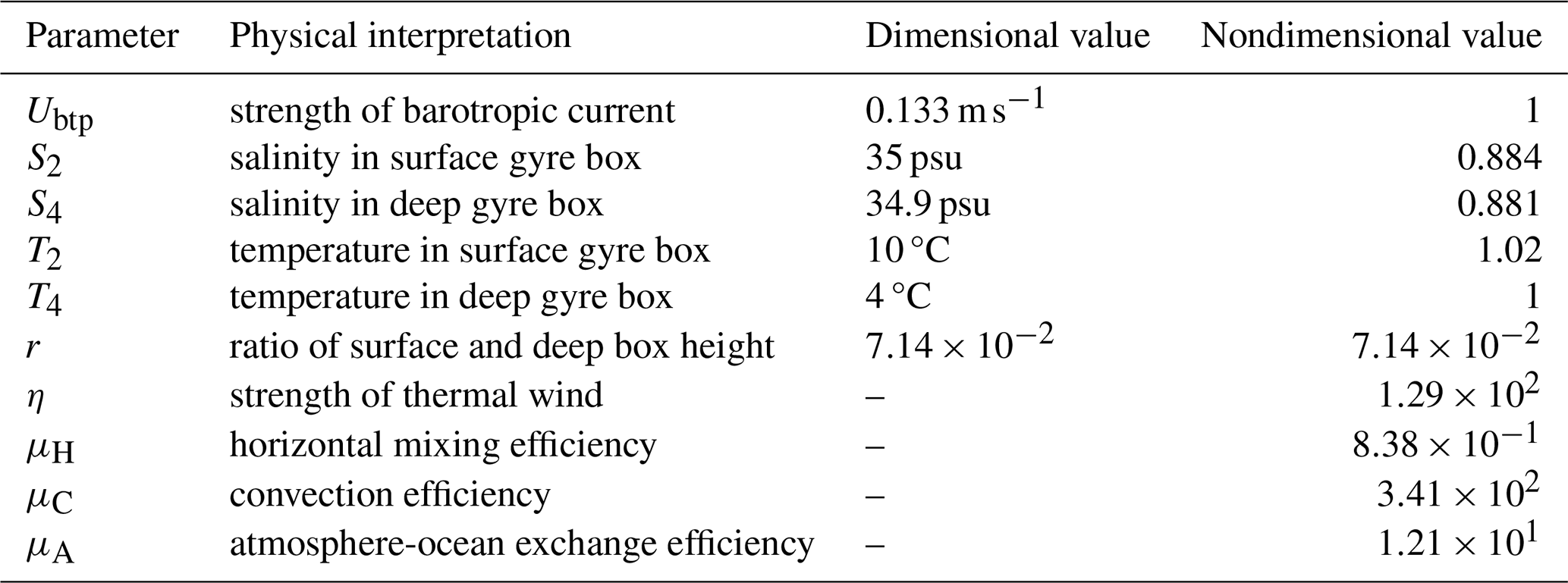
Table 1 Prescribed parameters of the model (Eq. 1). We use the parameter values of BS14 (their Table 1, here Table A1) to compute the parameter values for our non-dimensionalized model. Their parameter estimates are based on observations and expert assessment. The non-dimensionalization introduces some additional dimensionless parameters (η, μ_H, μ_C, and μ_A), for which no dimensional values are given for lack of interpetability (see Appendix A and Table A2).

The magnitude of the noise in Eq. (1) is determined by the noise variance σ_X and correlation time scale τ_X. When studying the effect of noise on the system, we vary the strength up to σ_S=0.5 psu and σ_F=1 m yr⁻¹ to compensate for the lack of seasonality in the model. To some extent, these large amplitudes can then simulate the effect of an anomalously wet, dry, fresh or saline year on the transport of the gyre. We select the correlation timescale τ_S=1 year (unless specified otherwise) to represent a multi-year mode of variability. This means that the modelled stochastic changes in the gyre salinity have a timescale of years, corresponding to the timescale of the Great Salinity Anomalies and driven by variations in e.g. sea ice cover. Conversely, we choose τ_F=90 d (unless specified otherwise) to represent a quasi-seasonal precipitation variability. It is worth nothing here that S₂ and consequently the noise term ζ_S are influenced by nonlinear prefactors in a way that F and ζ_F are not. We discuss the significance of this difference in Sect. 4.2.

The maximum values of the noise amplitude σ_S and σ_F were chosen to be quite high to gain a mechanistic understanding of the processes at play and to induce transitions within the system. As the model is highly conceptual, these variables should not be interpreted as realistic values of intrinsic noise in the climate system, but instead considered as high but not unrealistic given the simplicity of the conceptual model. The chosen values cause convection to collapse with a realistic frequency and are therefore not deemed too high. We discuss this further in Sect. 4.2.

2.2 Methods

We use two versions of the model (Eq. 1) in our analysis, as outlined above. When performing the bifurcation analysis (Sect. 3.1 and 3.2), we use the deterministic system. The stochastic version of Eq. (1) is used in the simulations where noise is applied to the system (Sect. 3.3 and 3.4).

2.2.1 Bifurcation analysis

The Julia continuation software BifurcationKit.jl (Veltz, 2020) was used to calculate bifurcation diagrams of the deterministic version of the system (Eq. 1) described in Sect. 3.1. The standard pseudo-arclength continuation (PALC) algorithm was used with Newton tolerances ranging from 10⁻⁹ to 10⁻¹¹, a minimum arclength of 10⁻¹⁰ and a maximum arclength ranging from 10⁻⁵ to 10⁻⁶. These values were varied slightly between continuations to ensure that the resulting diagrams were all in qualitative agreement about the structure of equilibria and bifurcations. Continuations were performed with S₂, F and T₂ as control parameter. In all results shown, the nondimensional model was used for calculations. After analysis units were converted back to dimensional units for ease of interpretation. Furthermore, in order to determine relevant parameter regimes for further analysis, a two-parameter (codim-2) continuation was performed in Sect. 3.2. Here, the bifurcation points that were found with S₂ as control parameter were continuated with F as control parameter. This provides an overview of the system's stability landscape as a function of these two parameters.

2.2.2 Simulations

The stability of the stochastic system (Eq. 1) was studied by time integration. These integrations were performed with the Julia library DifferentialEquations.jl (Rackauckas and Nie, 2017a, b). The built-in Euler-Maruyama method for stochastic differential equations was used with 3650 timesteps per year. The model was given 10 years of spin-up time. After this period the model was run for 5000 years unless specified otherwise. The values of the gyre transport M (Eq. 3) were averaged for every model year and only these average yearly values were used in further analysis. To quantify how long shutdowns of convection last, residence times in the non-convective state were calculated. As a non-convective state is associated with low gyre transport, the gyre was considered to be in a non-convective state when its yearly averaged transport M was less than 21 Sv for at least one year. When this was the case, the residence time in the non-convective state was calculated by counting the number of years that the gyre was in this state before transitioning back to a convective state. Kernel densities of the full time series and the residence times were estimated with KernelDensity.jl (Byrne, 2024) to visualize the long term behavior of the model. Lastly, the time the gyre spent in convective and non-convective states was quantified by the state ratio R, defined as

$$\begin{array}{}\text{(4)}& R={\displaystyle \frac{n_{\text{convection}}}{n_{\text{total}}}},\end{array}$$

where n_convection is the number of years the gyre is in a convective state with high transport M and n_total is the total length of the time series. When R=1, the gyre is in a convective (high transport) state for all model years, whereas when R=0 the gyre is in a non-convective (low transport) state for all model years.

3 Results

To understand the behavior of the subpolar gyre in the deterministic model, we performed a bifurcation analysis with three different control parameters: the gyre salinity S₂ and temperature T₂, and the freshwater forcing F. We vary the gyre salinity and temperature because changes in Greenland Ice Sheet runoff and precipitation will affect the salinity and temperature of the gyre current. Similarly, changes in precipitation in the center of the SPG region will have an effect on the density of the SPG's convective core. Varying these two control parameters thus allows us to study the effect of changes in the gyre's salinity budget on its circulation.

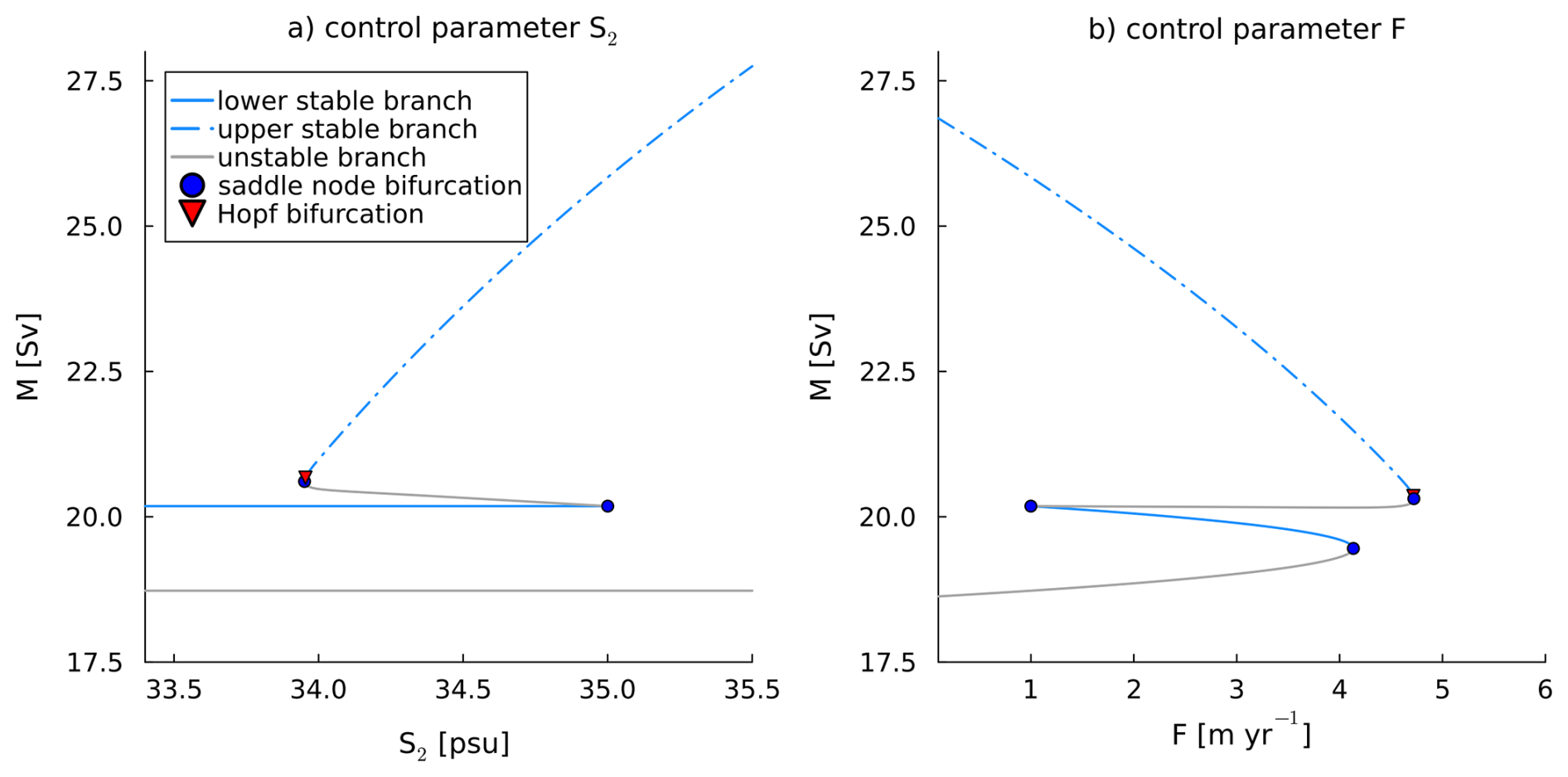
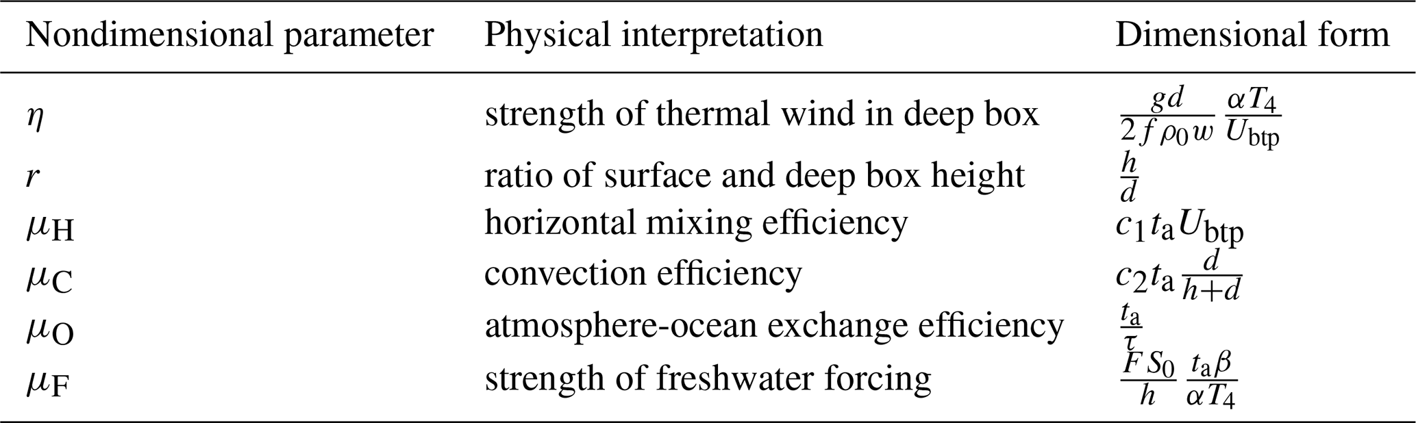
Figure 2 Bifurcation diagrams with gyre salinity S₂ and freshwater forcing F as control parameter and total gyre transport M on the vertical axis. Bistable regions were found between approximately 34 and 35 psu (S₂) and 1 and 4 m yr⁻¹ (F).

The results of this analysis are presented in Sect. 3.1. Building on these results, the behavior of the deterministic model is categorized into three regimes in Sect. 3.2. The behavior of the stochastic model under several noise levels in the gyre salinity is shown in Sect. 3.3. Lastly, we discuss the behavior of the model under various other combinations of noise in Sect. 3.4.

3.1 Single-parameter bifurcation analysis

A bifurcation diagram with the gyre salinity S₂ as control parameter is shown in Fig. 2a. The solutions are organized into two stable branches, connected by a double fold. For low values of S₂ the gyre transport is constant, with M≈20 Sv. This low-transport stable branch ends in a saddle node bifurcation at S₂=35 psu. The upper stable branch starts with a Hopf bifurcation, which is followed very closely by another saddle node. The transport of the upper branch is not constant, but increases in value as S₂ increases. An unstable branch connects the two stable branches.

The sensitivity of the gyre to the freshwater forcing F is shown in the bifurcation diagram in Fig. 2b. As in Fig. 2a, a double fold can be seen, consisting of two stable branches connected by an unstable branch. The lower stable branch terminates at a value of F=1.00 m yr⁻¹ on the left end and at F=4.13 m yr⁻¹ on the right. The higher stable branch terminates in a Hopf bifurcation which is accompanied by a saddle node bifurcation on the unstable branch very close to the Hopf bifurcation, similar to what was found with S₂ as control parameter. Bifurcation diagrams with T₂ as control parameter were also computed, but no bistabilies in a relevant parameter regime were found.

In our analysis, we found a Hopf bifurcation very close to a saddle node bifurcation for a wide range of parameters. This feature, together with zoomed-in figures of the region, is discussed in Appendix B. Since these Hopf bifurcations do not affect the results, they will not be discussed further in the main text.

The two stable branches that appear in the bifurcation diagrams (Fig. 2) represent different modes of gyre behavior in the model: the upper branch consists of solutions with convection, whereas the lower branch consists of solutions without convection. This can be deduced from the density differences between the different boxes of the model for the different branches (shown in Appendix Fig. C1 with S₂ as control parameter). When the vertical density difference σ₁−σ₃ is zero, which is the case for the upper branch, there is continuous overturning between boxes 1 and 3. This leads to large horizontal density differences and hence a strong baroclinic contribution to the gyre transport. In this convective regime the four-box model is effectively reduced to three boxes.

When the vertical density difference σ₁−σ₃ is negative, as is the case in the lower branch, the vertical boxes are stably stratified and no convection can occur. The lower cylindrical box is therefore fully connected to the lower annular box and the density difference between the two deep boxes is equal to zero. Consequently, there is no baroclinic contribution to the deep current U_d and the strength of the gyre is fully determined by the density difference between the upper two boxes and the barotropic current. Essentially, in this non-convective regime the four-box model is reduced to a two-box model.

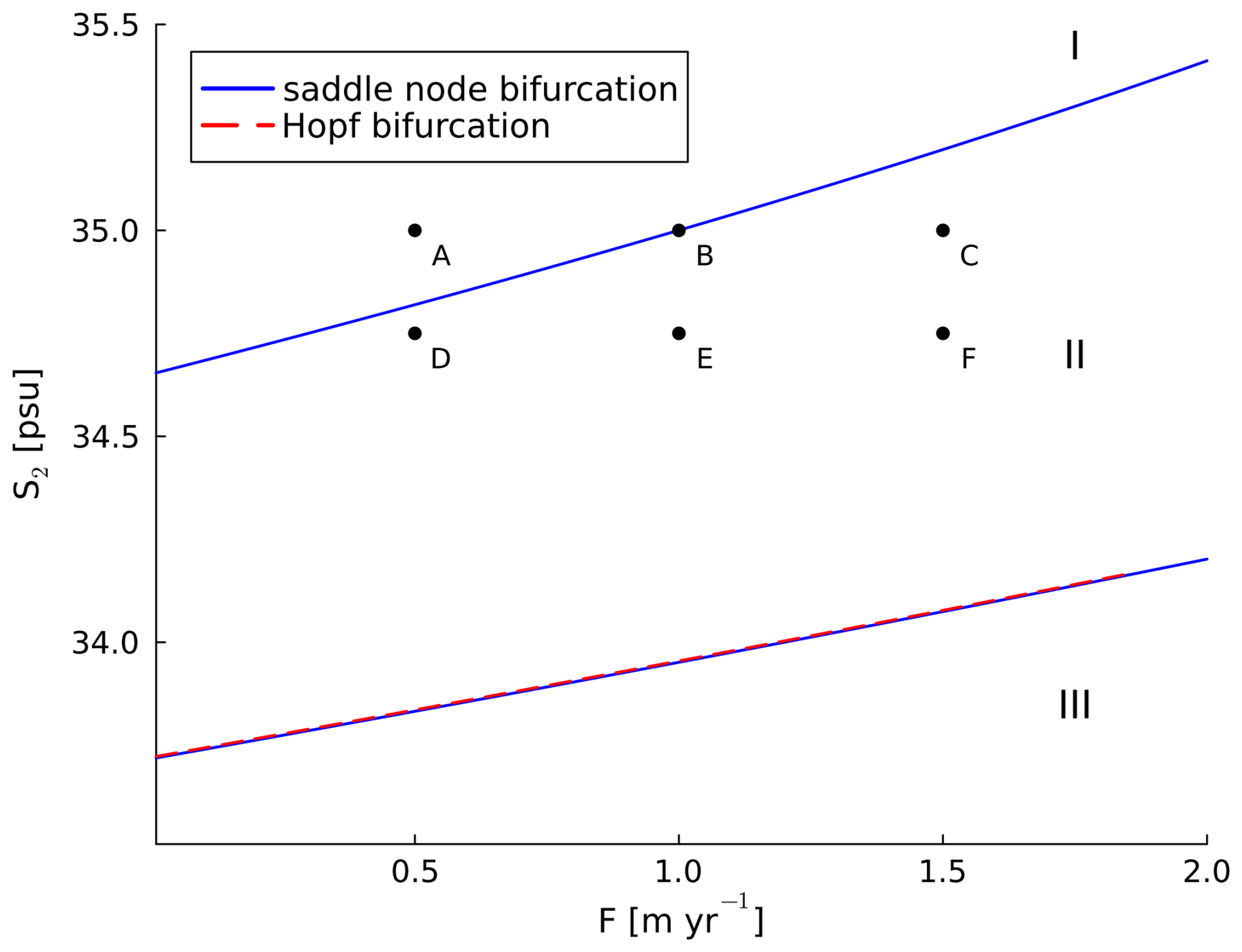
Figure 3 Two-parameter bifurcation diagram in the parameter range $\mathrm{0}<F<\mathrm{2}$ m yr⁻¹, 33.5 $<S_{\mathrm{2}}<\mathrm{35.5}$ psu. The three dynamical regimes are denoted by roman numerals I–III: regime I is monostable and convective, regime II is bistable, and regime III is monostable and non-convective. Points A to F are points in (S₂, F)-space that were used as parameter values in the time integrations performed in Sect. 3.3.

3.2 Model regimes

In order to understand how changes in both gyre salinity S₂ and freshwater forcing F affect the stability of the gyre, a two-parameter continuation was performed. The two saddle nodes and one Hopf bifurcation were continuated in a relevant parameter regime, which is defined here as a regime with $\mathrm{0}<F<\mathrm{2}$ m yr⁻¹ and 33.5 $<S_{\mathrm{2}}<\mathrm{35.5}$ psu.

This two-parameter diagram (Fig. 3) shows for which parameter values certain types of behavior can be expected. The lines in this figure represent the location of the bifurcation points, rather than the equilibrium solutions. If a vertical transect at a given value of F is followed for increasing values of S₂, first a saddle-node and Hopf bifurcation are encountered. For higher values of S₂ another saddle-node is found. Above this last saddle-node there are no bifurcation points in this parameter range. Such transects with constant F and varying S₂ were shown previously in Fig. 2a (for F=1 m yr⁻¹). The vertical region between the blue lines representing saddle-node bifurcation in Fig. 3 corresponds to the bistable region in Fig. 2a. Similarly, horizontal transects in Fig. 3 are an extension of the results shown in Fig. 2b (for S₂=35 psu), but for realistic values of F only one saddle node is encountered.

Based on Fig. 3, three different model regimes can be distinguished. The first regime (denoted I) is monostable and convective. The gyre model is only in this regime for sufficiently high values of S₂. Solutions in this regime correspond to high values of gyre transport M. In the other monostable regime (III) there is again only one stable solution, but for this solution there is no convection in the SPG. This corresponds to low values of the gyre transport M. In the intermediate regime (II) there are two stable solutions, one with and one without convection. Formally, a fourth region can be distinguished between regions II and III. This region is demarcated by the Hopf bifurcation and the lower saddle node bifurcation. However, this region is very small and since we do not find periodic orbits associated with the Hopf bifurcation (see Appendix B), we do not consider it in our analysis.

According to the reference values that were used in BS14, the subpolar gyre's current state is on point B in Fig. 3 (F=1 m yr⁻¹, S₂=35 psu), within the bistable regime II. It is therefore potentially susceptible to changes in precipitation, hydrography and circulation, as changes in F or S₂ may lead to a transition to a non-convective state. In other words, the gyre can exhibit tipping behavior.

3.3 Noise in the gyre salinity

To study if noise can indeed induce transitions between convective and non-convective states, six different sets of parameter values in (S₂,F)-space were selected, as indicated in Fig. 3 with letters A–F. The stochastic model (Eq. 1) was then time-integrated for long run times to study the effect of noise for different values in parameter space. The six points A–F were chosen to be in a region in (S₂,F)-space that is the boundary between regimes I and II, such that points in both the monostable convective and the bistable convective regime are considered. Within our model context, the present day subpolar gyre region has a gyre salinity S₂ of 35 psu and freshwater forcing F of 1 m yr⁻¹ (BS14). Point B in Fig. 3, representing these present-day values, is defined as the reference forcing.

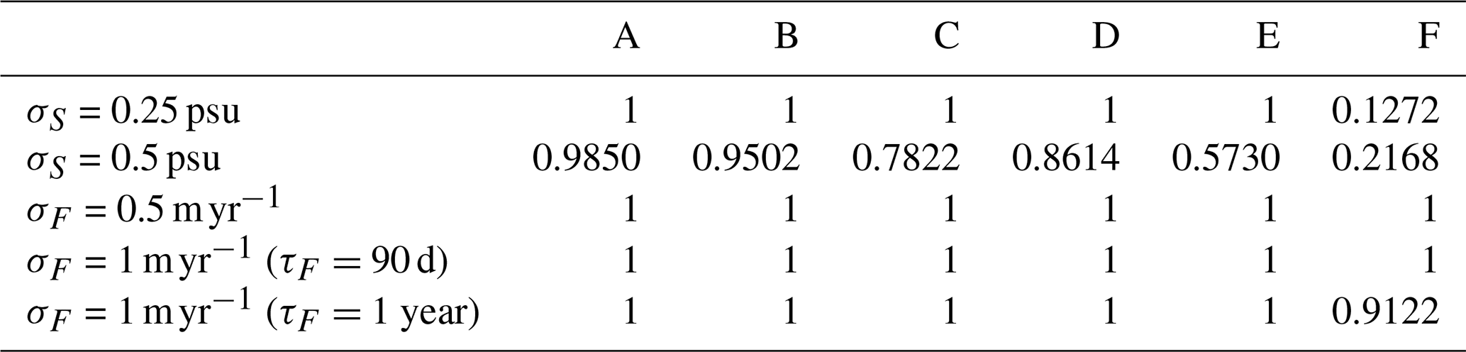
Table 2 State ratio R (Eq. 4) for different noise levels and parameter values in (S₂,F)-space, as defined in Fig. 3. Point A corresponds to S₂=35 psu, F=0.5 m yr⁻¹; point B to S₂=35 psu, F=1 m yr⁻¹; point C to S₂=35 psu, F=1.5 m yr⁻¹; point D to S₂=34.75 psu, F=0.5 m yr⁻¹; point E to S₂=34.75 psu, F=1 m yr⁻¹; and point F to S₂=34.75 psu, F=1.5 m yr⁻¹.

The other five points hence span variability around present-day values of the parameters, as well as possible deviations from the reference forcing. Point A (S₂=35 psu, F=0.5 m yr⁻¹) represents a reference salinity forcing and a lower-than-reference freshwater forcing (i.e. precipitation). Point C (S₂=35 psu, F=1.5 m yr⁻¹) represents the same salinity forcing as A and B and a higher-than-reference freshwater forcing. Points D, E and F all have a lower-than-reference salinity and the same increasing freshwater forcing as points A, B and C. No points with higher-than-reference salinity were tested, since nearly all external changes to the gyre current serve to decrease its salinity.

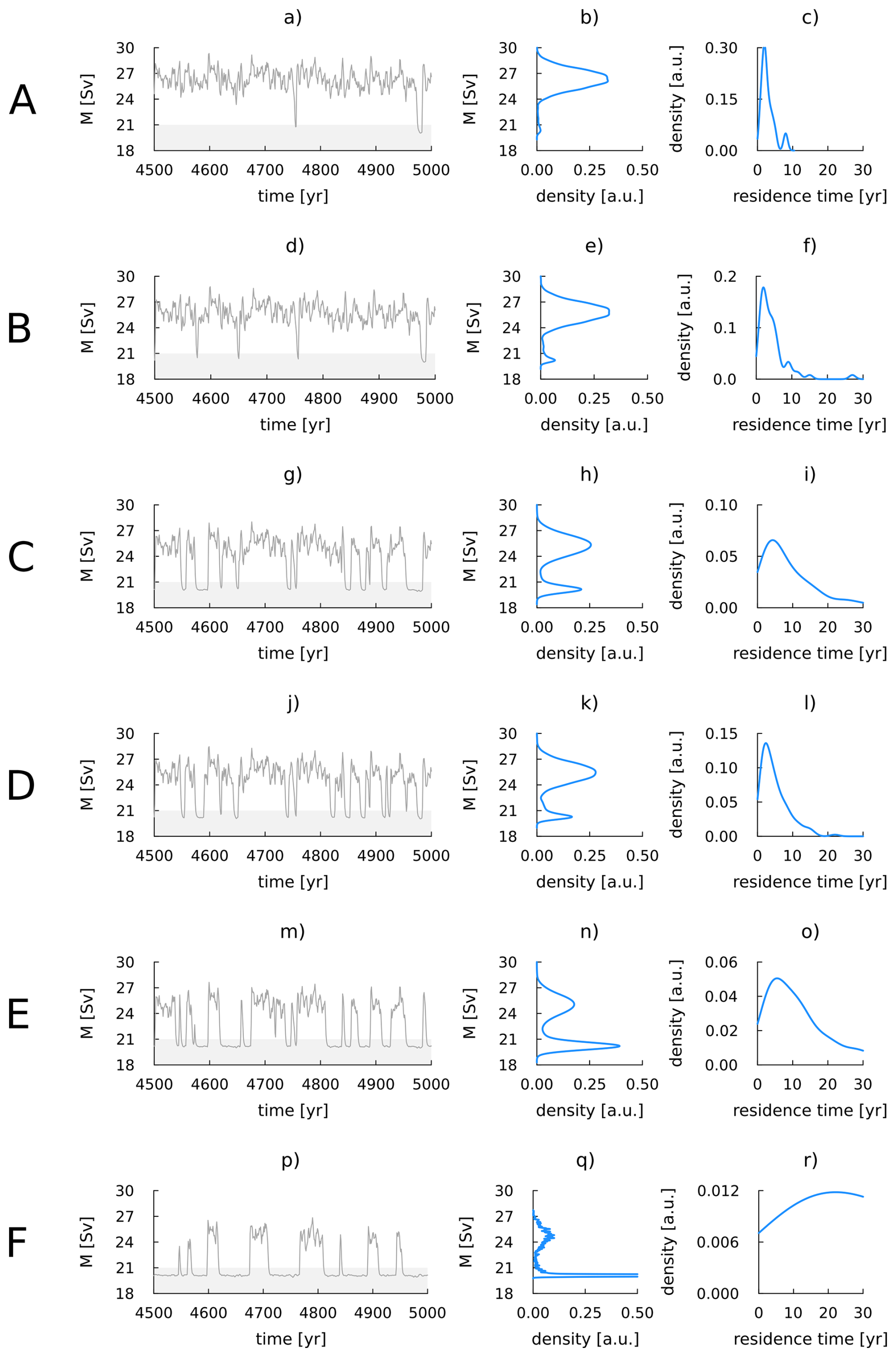
Figure 4 Time series and statistics of time integrations of the stochastic SPG model with noise level σ_S=0.5 psu. The letters A to F on the left denote the sets of parameter values in (S₂,F)-space, as defined in Fig. 3. Subfigure (a) (d, g, j, m, p): time series of gyre transport M for the last 500 model years. The gyre is considered to be non-convective when M<21 Sv, indicated by grey shading in the time series. Subfigure (b) (e, h, k, n, q): kernel density of the gyre transport M, showing the relative occurence of years with and without convection. Subfigure (c) (f, i, l, o, r): kernel density of time spent in the state with no convection. Note that the y-axis of this right column is scaled differently for every plot. All integrations were performed for 5000 model years and yearly averaged values of these 5000 model years were used to calculate the kernel density estimates.

The main results from the integrations with noise applied to the gyre salinity (σ_S=0.5 psu) are summarized in Fig. 4. The final 500 years of the time series are shown, as well as kernel density estimates of the total time series and the time spent in the non-convective state. In addition, values of the state ratio R (Eq. 4) for integration with σ_S=0.25 psu (not shown in Fig.) and σ_S=0.5 psu are shown in Table 2 as a measure of how much time the gyre spends in a convective state. Clearly, the integrations for the six parameter sets A–F exhibit different behavior. Changing the values of the parameters in (S₂,F)-space can have profound influences on the dynamics of the gyre.

A first observation is that increasing the freshwater forcing F always leads to less convection in the gyre. For parameter set A, the gyre is almost never in a state without convection, as can be seen in Fig. 4b. As F increases, the amount of years spent in the non-convective state increases. This can be seen in the small bump in the kernel density of the gyre transport around 20 Sv for parameter set B (Fig. 4e) and much more clearly for parameter set C (Fig. 4h). Similar behavior can be observed in the progression from parameter set D to F. The gyre spends most of its time in the non-convective state for parameter set F (Fig. 4q and R<0.5, Table 2).

Similarly, decreasing the background salinity S₂ always leads to an increase in the amount of years without convection. When comparing cases with the same freshwater forcing but different salinity (A versus D, B versus E, C versus F), the gyre always spends fewer years in the convective state for the case with lower salinity. Taken together, increasing F and decreasing S₂ destabilizes the gyre's convection, whereas decreasing F and increasing S₂ stabilizes it. The opposing sign of these two effects is not surprising, as both decreasing S₂ and increasing F reduces salinity levels in the gyre.

These destabilizing factors increase the total amount of years spent in the non-convective state, as well as increasing the average time a non-convective period lasts. The latter is shown in the rightmost column of Fig. 4. When the gyre is stable and spends most of its time in a convective state, excursions to the non-convective state are short, typically lasting much less than 10 years. This can be seen in, for example, cases A (Fig. 4c) and D (Fig. 4i). As convection in the gyre destabilizes, the kernel density estimate of time spent in the non-convectives state broadens to longer times. The peak also shifts to longer residence times. This is most visible for case F (Fig. 4r) and to a lesser extent also for cases C and E (Figs.4i and o).

It is worth noting that even in the least stable case studied here (F), the gyre never becomes fully non-convective. The length of the non-convective periods increases and most of the time is spent in the non-convective state, but there are still many convective episodes. Qualitatively, the gyre transitions from a convective (high transport) state with non-convective (low transport) episodes to a non-convective (low transport) state with convective (high transport) episodes. In the time series (Fig. 4p) these episodes appear as “excitations” from a more stable low transport mean state. However, both branches are still stable solutions (Sect. 3.1).

These results, where the amplitude of the applied noise is σ_S=0.5 psu, are summarized in the second row of Table 2. The destabilization of the gyre's convection is represented here by a decrease in state ratio R. Interestingly, for this noise level, convection ceases in all cases studied at least for some years. Even case A, for which the deterministic parameter values are clearly in the monostable convective regime (Fig. 3), has rare events during which the convection collapses. Such events are not completely unexpected, as the applied noise amplitude (0.5 psu) is greater than the distance from the regime boundary (approximately 0.2 psu). This shows that being in a “safe” monostable parameter regime does not guarantee that convection in the gyre will never destabilize under stochastic forcing.

Conversely, when the parameter values in (S₂,F)-space are far in the bistable regime, a low noise level can result in few transitions and therefore a strongly non-convective gyre. This is the case for parameter set F when σ_S=0.25 psu (Table 2): here, because the applied noise level is low, transitions between states are rare and the gyre can end up spending most of its time in a non-convective state. This phenomenon seems to be governed mostly by chance and not by the stability of the system, as the basin of attraction of the convective branch is much bigger than that of the non-convective branch (Fig. 2).

We performed additional simulations (not shown) to confirm that the gyre fully transitioned from a convective to a non-convective state during shutdowns of convection. In these simulations we identified events where convection stopped, defined (as above) as a yearly average transport M of less than 21 Sv, for more than one year. We then took the state of the gyre (the temperature and salinity of boxes 1 and 3) in the last year before convection recovered as an initial condition and continued the simulation without any noise forcing. These experiments demonstrated that for parameter sets B to F convection remained in a low-transport state, confirming that the collapses of convection discussed above are transitions from one state to the other. However, for parameter set A the gyre was able to recover to a high-transport state without additional noise forcing, indicating that the rare collapses of convection for this parameter set are noise events and not transitions to a non-convective state. As parameter set A is in the monostable convective regime and the state with no convection is unstable, this is an expected result.

3.4 Noise in freshwater forcing

Both the gyre salinity S₂ and the freshwater forcing F can exhibit variability. To study the effect of the latter, the model was also integrated with added noise in the freshwater forcing instead of noise in the gyre salinity. The state ratios R from these integrations (σ_F=1 m yr⁻¹) are summarized in Table 2. These results show a drastically different picture than those discussed above: for virtually all of the performed simulations, the gyre always remains in a convective state with high transport.

This is somewhat surprising. The noise amplitude σ_F=1 m yr⁻¹ is twice that of the noise applied to S₂ shown in Fig. 4, yet no transitions between the convective and non-convective state are observed when the timescale τ_F of the noise in F is 90 d. Even when τ_F is increased to one year, the gyre only stops convecting a few times in case F (Table 2). In this scenario, the gyre again only has non-convective episodes for a high value of F and a low value of S₂. This is in line with the results shown above, in which convection in the gyre was the least stable for case F. These simulations indicate that the convection in the SPG is less sensitive to noise in the freshwater forcing than to noise in the background gyre salinity.

In all results thus far presented, noise was only applied in either the gyre salinity or the freshwater term. Adding noise in both terms simultaneously could have a different effect on the gyre's behavior. To rule out this possibility, integrations were performed with various combinations of the noise amplitudes σ_S and σ_F. The results of these integrations are shown in Fig. 5. Clearly, σ_S is the main driver of noise-driven transitions. The rightmost columns have the lowest value of R for all cases. In other words, as the noise in S₂ increases, the gyre spends more time in a non-convective state.

Contrastingly, increasing the noise in the freshwater forcing does not seem to influence the behavior of the gyre much. For cases A, B, C, and D, there is no clear decrease in R as σ_F increases. For the other cases, large noise amplitudes in the freshwater forcing slightly increase the amount of time spent in the non-convective state. This can be seen in the hatched cells corresponding to high values of σ_F for parameter E (σ_S=0.3 psu) and F (σ_S=0.2 psu). A possible explanation for this is that these parameter sets are far in the bistable regime, making transitions between states are easier here. The additional forcing of σ_F can help induce a transition to a non-convective state, but only when σ_S is sufficiently high. In other words, high noise in the freshwater forcing can lower the threshold of noise in salinity that is required to stop convection in some cases. Overall, applying noise to the gyre salinity has a much greater effect than applying it to the freshwater forcing. This low sensitivity to noise in the freshwater forcing is discussed extensively in Sect. 4.2.

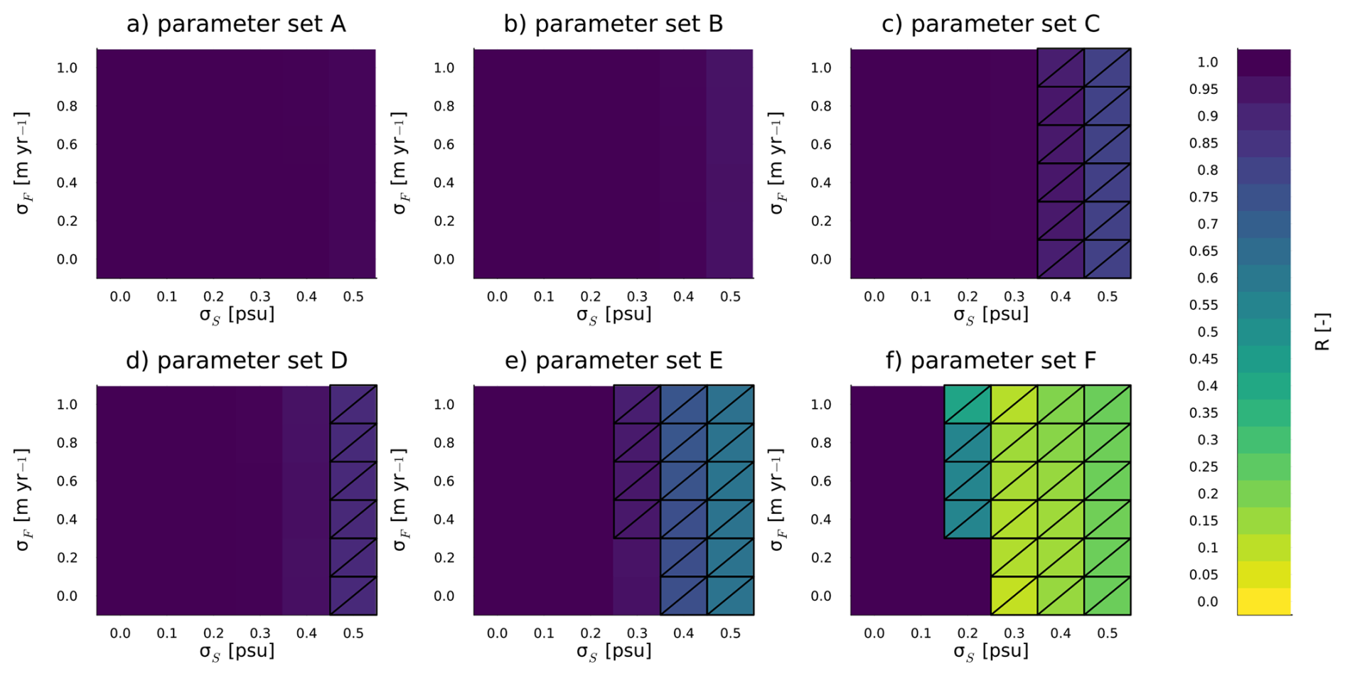
Figure 5 State ratio R for different combinations of noise amplitudes σ_S, σ_F for the six parameter sets (subfigures a–f). Each value of R was calculated for every combination from a time integration of 10000 years. Cells are hatched when R<0.95, indicating that the gyre spent more than 5 % of the model years in a nonconvective state.

4 Discussion and Conclusions

We used a conceptual model of the SPG to investigate the occurrence of periods with and without convection, and how the presence of noise in salinity and precipitation influences the stability of convection. In this section, we summarize the results from the bifurcation analysis in Sect. 4.1. This is followed by a discussion of the model's high sensitivity to noise in the gyre salinity in Sect. 4.2. Some limitations of the used model are outlined in Sect. 4.3 and lastly, the results presented here are discussed in the context of the SPG's resilience in Sect. 4.4.

4.1 Bifurcation structure

In Sect. 3.1 we showed that there is a bistability in the gyre's transport M for certain (combinations of) values of S₂ and F. This is in agreement with the results found in BS14. The main difference between our results and those in BS14 is the width of the hysteresis: in our results, bistabilities are present for a larger range of parameter values. This is caused by the absence of a seasonal cycle in the forcing of the model (Eq. 1) and is discussed further in Sect. 4.3.

The bifurcation structure of the bistability is a double fold, and the two branches of these folds exhibit very different behavior. The high transport (M) branch corresponds to a gyre with permanent convection, whereas the low transport branch corresponds to a gyre with no convection. Based on the parameter values in (S₂,F)-space, in Sect. 3.2 we distinguished three different regimes for the gyre's dynamical state: a monostable convective, a bistable, and a monostable non-convective regime. In and close to this bistable regime, noise can induce transitions from one state to the other. No region of bistability was found when using T₂ as the control parameter. The SPG is therefore, at least in this model, much more sensitive to haline pertubations in the surface gyre boxes than to oceanic temperature pertubations.

4.2 Strong sensitivity to noise in gyre salinity

In Sect. 3.3 and 3.4, we studied the effect of noise on the SPG's behavior. We found that convection in the gyre can temporarily collapse due to stochastic forcing. The likelihood and severity of these collapses is strongly influenced by the choice of parameters in (S₂,F)-space. Decreasing the surface current salinity S₂ and increasing the freshwater forcing F both destabilize the SPG and increase its sensitivity to noise-induced collapses of convection. As the gyre destabilizes, a state without convection occurs more often and the time that is spent in each non-convective period increases. However, even in the least stable parameter regime studied here convection in the gyre never fully collapses, and it is always possible to restart convection stochastically. Similarly, when the gyre is in a monostable convective regime, convection can still ocassionally collapse and recover stochastically. However, in this case the SPG does not transition to a non-convective state.

These findings can be interpreted in the context of large deviation theory. A system under stochastic forcing is expected to experience arbitrarily large deviations from its stable state over a long enough period of time (Freidlin and Wentzell, 2012). In a bistable system, the time spent in one of the two states before transitioning to the other depends on the strength of the noise process and the height of the barrier seperating the two states (Bouchet and Reygner, 2016). By choosing the different parameter sets B to F we effectively change the height of this barrier, thereby modulating the probability of a state transition and the amount of years the gyre spends in a convecting state. This is not the case for parameter set A; here, the gyre is in a monostable state, and the occasional collapses of convection we observe in this case are more accurately described as noise events than as full state transitions. These events are an example of wandering unimodality (Kuhlbrodt and Monahan, 2003), where the addition of noise allows the system to “wander” into a regime that is not stable in a deterministic sense.

A striking result is that noise in the freshwater forcing F does not have nearly as much of an influence on the SPG's behavior as noise in the gyre salinity S₂. Transitions are almost exclusively driven by noise in the salinity. A possible reason for this result is that the noise terms are applied to different boxes of the conceptual model: the noise in F is applied to the inner surface box 1, whereas the noise in S₂ is applied to the surface current box 2. The stochastic freshwater forcing ζ_F is therefore distributed over a larger volume than the stochastic salinity forcing ζ_S and the effective applied concentration is lower. This could partially explain the relatively small effect of adding noise in F. However, as salinity is not conserved in this model, it is hard to quantify the effect of these different volumes.

Another possible explanation could be that the response of the convection dynamics to noise in the gyre salinity S₂ is nonlinear, due to the interaction via the strength of the boundary current. In the model (Eq. 1), the freshwater term $-F+{\mathit{\zeta }}_F$ is added linearly to the rest of the terms, whereas the salinity term S₂+ζ_S is multiplied by the surface current strength U_s, making it a strongly nonlinear term. This difference is, however, not necessarily caused by the assumptions of the simple model. It reflects the strong nonlinearity of the mechanism by which salinity anomalies are transported from the boundary current to the convective core of the SPG. It seems likely that the different impact of adding noise in S₂ and F is, at least in part, caused by the baroclinic reponse of the circulation and its impact on the salinity anomalies in the convective regions of the SPG.

Regardless of the mechanism, there is ample evidence to support the hypothesis that convection in the SPG is more sensitive to variability in the salinity of the boundary current than to variability in the precipitation. Yashayev (2024) identified the freshening of the Labrador Sea, caused by a release of low-salinity water from the Beaufort Gyre, as the main cause for the 2023 shutdown of convection in the region. Similarly, Gelderloos et al. (2012) argued that the Great Salinity Anomaly of 1968 initiated the shutdown of convection in 1969. In addition, they found the advection of saltier watermasses to be one of the reasons convection restarted in 1972. The passage of such an anomaly through the gyre can be seen as a stochastic deviation from the gyre's mean salinity. The modelled gyre's response to these anomalies by switching from a convective to a non-convective state is therefore in agreement with the observed collapse of convection in the gyre during GSAs. Conversely, we are not aware of any previous work that indicates that variability in precipitation in the region contributes meaningfully to the variability of convection.

It is remarkable that the highly idealized BS14 model can reproduce these results. This is an indication that this model, simple as it is, captures some of the main physical processes that are at play in the SPG, substantiating the results presented in their work and here. It also emphasizes the continued relevance of using simple box models in oceanographic research.

Ultimately, the behavior of the gyre in this simple stochastic model qualitatively and quantitatively matches the observed behavior, despite the noise being on the high end of realistic values. For parameter set B, representing current oceanographic conditions, the gyre spends approximately 5 % of its time in a non-convective state. Considering the frequency of collapses of convection that were observed in the previous half century (Sect. 1;  Lazier, 1980; Dickson et al., 1988; Belkin et al., 1998; Biló et al., 2022; Yashayev, 2024) this is a realistic value. For this reason the used values of noise in especially the gyre salinity are not deemed too high, given the simplifications and assumptions in the model itself (see discussion in Sect. 2.1).

It would be interesting to add an additional noise term in the atmospheric temperature, as anomalous atmospheric conditions have been linked to shutdowns of convection in the Labrador sea (Gelderloos et al., 2012; Yashayev, 2024). However, the autonomous model setup used here is unsuitable for this. Because there is no seasonality in the autonomous model, the rate of convection is directly set by the atmospheric temperature T₀. Small stochastic deviations from T₀ would therefore have a direct and major effect on the rate of convection and the gyre's transport. In the more subtle original BS14 model with a seasonal cycle, noise in the atmospheric temperature could be interpreted as year-to-year variability. However, the bifurcation analysis could only be performed with an autonomous model and therefore, to keep all results consistent with each other, we only analyzed the autonomous model. In the following subsection we discuss how not including a seasonal cycle in the simulations affects the conclusions that can be drawn from them.

4.3 Limitations of the conceptual model

All results in this paper were derived from the adjusted model (Sect. 2.1) of convection in the Labrador Sea. Although conceptual models can provide useful results and ease the interpretation of other model studies, they are highly simplified and their results should be interpreted as such. In addition, all analysis was based on an autonomous version of the model. This model does not have a seasonal cycle and might therefore behave quite differently from the non-autonomous original model. Convection in the Labrador sea is highly seasonal and only happens in winter when atmospheric temperatures are sufficiently low. By removing this seasonality the model becomes much less subtle, raising the question if the results presented here realistically represent convection in the SPG.

In order to quantify how removing the seasonal cycle affects the results, a non-autonomous version of the model with a seasonal cycle was simulated with the same stochastic forcings in S₂ as the autonomous model. The results of the simulations with noise applied to the gyre salinity are shown in Supplementary Fig. C2. As before, convection in the gyre becomes less stable as S₂ decreases and F increases. In addition, the years that are spent in the convective and non-convective states (second column) are distributed approximately the same for the same parameter sets in the non-autonomous and autonomous states. The main difference between the non-autonomous and automous models is that in the non-autonomous model, the gyre typically spends less time in a non-convective state before returning to a convective state (rightmost column of Supplementary Fig. C2). The seasonal cycle in atmospheric temperature makes conditions favorable for convection in winter and extremely unfavorable in summer. On long timescales, this causes the gyre to spend approximately the same time in both states, but the transitions between states become more frequent. This is reflected in the shorter residence times.

Overall, the results from the autonomous and non-autonomous model integrations are in good qualitative correspondence. This indicates that the underlying bifurcation structure of the two models is similar and substantiates the results presented in this article. The fact that such a simple model can replicate collapse and restart of convection in the gyre with simple stochastic forcing is an indication that this is a fundamental mode of SPG behavior.

Only the impact of changes in parameter values on the SPG's behavior was studied here. These are of course not the only factors that can change the stability of convection. For example, one can imagine that the ratio between the depths of the two boxes has some influence on the stability of convection in the gyre. This was investigated in some detail in BS14, but it would be interesting to formalize their analysis and use continuation software to systematically study the importance of geometric effects. A simple model with variable convection depth would be a much more realistic description of year-to-year convection in the Labrador sea, allowing for an analysis of the effects of preconditioning of the water column between years.

4.4 Resilience of the SPG

Based on the results from the simple model presented here, we conclude that a permanent collapse of convection in the North Atlantic subpolar gyre is unlikely under current oceanographic and atmospheric conditions. Convection may occasionally collapse due to stochastic forcing in the salinity budget, but it can always be recovered. As the gyre's salinity decreases and the freshwater forcing increases, convection in the gyre collapses more often and non-convective episodes last longer. However, in none of the studied parameter sets with different salinity and freshwater forcing does convection in the gyre stop altogether. Restart of convection is always possible.

This resilient quality of the SPG is not often found in studies that employ Earth System Models (ESMs). In most CMIP5 and CMIP6 models convection in the SPG does not restart after collapsing, although one model in the ensemble (NorESM-LM) is in principle able to simulate a recovery of convection (Swingedouw et al., 2021; Sgubin et al., 2017). Deep convection in the Labrador Sea was also found to be intermittent in a 12-model historical ensemble of EC-Earth (Brodeau and Koenigk, 2016). However, it should be noted that the results from most ESM studies cannot be compared directly to our results. We have assumed a non-changing background state (i.e. T₀ and U_btp were held constant), whereas most relevant ESM modelling studies investigate the response of the SPG to a changing climate. Based on this assumption we conclude that at least in this simple model convection in the SPG is stable to salinity pertubations in our current climate. This conclusion does not necessarily hold for other pertubations, such as changes in mean the atmospheric temperature. Investigating the response of a simple model to such changes is an interesting avenue for future research.

The other possibility is that collapse of convection is a much more frequent process than currently thought. This might be due to the relatively low availability of data, either from high complexity models or from observations. Simulating the climate with ESMs is time-consuming and expensive, and it is not feasible to obtain long time series of climate in the SPG region. It might be the case that convection spontaneously restarts when these models are run for a longer time. Alternatively, it is possible that CMIP5 and CMIP6 models do not capture the stochastic nature of convection in the Labrador Sea. Even in our current climate, convection in this region is not permanent but sometimes ceases and restarts during Great Salinity Anomalies and anomalous atmospheric conditions. Accurately modelling complex air-ice-sea interactions is complicated, and it is possible that these processes are not resolved fully in ESMs.

If the results here are taken at face value, collapse of convection in the SPG does not have to be permanent. It would be interesting to know what effect the switching between states of convection and no convection in the Labrador sea has on the stability of the AMOC. In AMOC stability studies, it is often assumed that the collapse of convection in one of the AMOC's convective basins is relatively permanent and a precursor to other changes (e.g. Neff et al., 2023 and references therein). The consequences of such a permanent collapse on AMOC stability are presumably different than when convection collapses and restarts again on a timescale that is fast for the AMOC. In addition, the relation between the SPG and the Greenland Ice Sheet and Arctic sea ice should be studied in more detail, as these systems provide much of the low-salinity water that can potentially destabilize convection in the gyre (Dukhovskoy et al., 2021; Malles et al., 2025).

In conclusion, further research is needed to conclusively determine how stable convection in the North Atlantic subpolar gyre really is. Moreover, more insight is needed into whether or not convection in ESMs can restart (or move to different regions), and how this relates to the AMOC strength. The interpretation of the collapse of convection as either a tipping point in the climate system or as a relatively common process induced by the stochastic nature of oceanic and atmospheric forcing continues to hold important scientific and societal relevance.

Appendix A: Derivation of the model

The model as described in BS14 consists of the definition of density

$$\begin{array}{}\text{(A1)}& \mathit{\sigma }=-\mathit{\alpha }T+\mathit{\beta }S,\end{array}$$

and the six coupled equations

$$\begin{array}{}\text{(A2)}& \begin{array}{rl}{\displaystyle }{U}_{\text{d}}& {\displaystyle }=U_{\text{btp}}-{\displaystyle \frac{gd}{\mathrm{2}f{\mathit{\rho }}_{\mathrm{0}}w}}({\mathit{\sigma }}_{\mathrm{4}}-{\mathit{\sigma }}_{\mathrm{3}}),\\ {\displaystyle }{U}_{\text{s}}& {\displaystyle }=U_{\text{d}}-{\displaystyle \frac{gd}{\mathrm{2}f{\mathit{\rho }}_{\mathrm{0}}w}}({\mathit{\sigma }}_{\mathrm{2}}-{\mathit{\sigma }}_{\mathrm{1}}),\\ {\displaystyle \frac{\mathrm{d}{T}_{\mathrm{1}}}{\mathrm{d}t}}& {\displaystyle }=c_{\mathrm{1}}{U}_{\text{s}}(T_{\mathrm{2}}-T_{\mathrm{1}})\\ {\displaystyle }& {\displaystyle }+{\mathit{\tau }}^{-\mathrm{1}}(T_{\mathrm{0}}-T_{\mathrm{0}}^{\text{amp}}\cos (\mathit{\omega }t)-T_{\mathrm{1}}],\\ {\displaystyle \frac{\mathrm{d}{S}_{\mathrm{1}}}{\mathrm{d}t}}& {\displaystyle }=c_{\mathrm{1}}{U}_{\text{s}}(S_{\mathrm{2}}-S_{\mathrm{1}})-F_{\text{s}},\\ {\displaystyle \frac{\mathrm{d}{T}_{\mathrm{3}}}{\mathrm{d}t}}& {\displaystyle }=c_{\mathrm{1}}{U}_{\text{d}}(T_{\mathrm{4}}-T_{\mathrm{3}}),\\ {\displaystyle \frac{\mathrm{d}{S}_{\mathrm{3}}}{\mathrm{d}t}}& {\displaystyle }=c_{\mathrm{1}}{U}_{\text{d}}(S_{\mathrm{4}}-S_{\mathrm{3}}).\end{array}\end{array}$$

The total horizontal volume transport by the flow can be expressed as

$$\begin{array}{}\text{(A3)}& M=U_{\text{s}}wh+U_{\text{d}}wd.\end{array}$$

Note that the (dimensional) parameter c₁ in our formulation is equal to c in Eq. (15) of BS14, such that

$$\begin{array}{}\text{(A4)}& c_{\mathrm{1}}=c^{*}{\displaystyle \frac{A}{V}}=c^{*}{\displaystyle \frac{\mathrm{2}\mathit{\pi }{r}_{\text{i}}h}{\mathit{\pi }{r}_{\text{i}}^{\mathrm{2}}h}}={\displaystyle \frac{\mathrm{2}{c}^{*}}{R}}.\end{array}$$

Here A denotes the area of the interface between box 1 and 2, and V the volume of box 1.

In the BS14 model convection between box 1 and 3 is not described with a prognostic equation. Instead, at every time step the density anomalies σ₁ and σ₃ are compared. When σ₁>σ₃, the two volumes are mixed by taking the volume-weighted average of the density of the two boxes.

We adjusted several aspects of this model. Firstly, in order to capture the convection process in a formal bifurcation analysis, it needed to be parameterized without discontinuities in time or parameter space. This was be done by employing a step-like function

$$\begin{array}{}\text{(A5)}& \mathcal{H}\left(x\right)={\displaystyle \frac{\mathrm{1}}{\mathrm{2}}}+{\displaystyle \frac{\mathrm{1}}{\mathrm{2}}}\tanh \left(kx\right),\end{array}$$

where k≫1 to ensure mixing between the boxes occurs instantaneously (e.g.  Dijkstra, 2005, pp. 70). In this study a value of k=10⁵ was used. The convection between box 1 and 3 was then implemented in the temperature and salinity flux equations, leading to the governing equation

$$\begin{array}{}\text{(A6)}& \begin{array}{rl}{\displaystyle \frac{\mathrm{d}{T}_{\mathrm{1}}}{\mathrm{d}t}}& =c_{\mathrm{1}}{U}_{\text{s}}(T_{\mathrm{2}}-T_{\mathrm{1}})+{\displaystyle \frac{d}{d+h}}{c}_{\mathrm{2}}\mathcal{H}({\mathit{\sigma }}_{\mathrm{1}}-{\mathit{\sigma }}_{\mathrm{3}})(T_{\mathrm{3}}-T_{\mathrm{1}})\\ & +{\mathit{\tau }}^{-\mathrm{1}}(T_{\mathrm{0}}-T_{\mathrm{0}}^{\text{amp}}\cos (\mathit{\omega }t)-T_{\mathrm{1}}),\end{array}\end{array}$$

and similar for the equations describing S₁, T₃, and S₃. Here c₂ (with c₂≫c₁, taken here as $c_{\mathrm{2}}/c_{\mathrm{1}}={\mathrm{10}}^{\mathrm{3}}$ m s⁻¹) is the efficiency of mixing due to convection, and h and d are the depth of the upper and lower box, respectively. Taking high values for both c₂ and k ensures that convective mixing between box 1 and 3 happens nearly instantaneously, in line with the implementation of convection in BS14. The convection terms are multiplied by the $d/(d+h)$ and $h/(d+h)$ to account for the different volumes of the boxes and conserve temperature and salinity during the convective mixing. The values of all dimensional parameters are shown in Table A1.

The resulting equations were non-dimensionalized by multiplying the temperatures by $\mathrm{1}/T_{\mathrm{4}}$ and the salinities by $\mathit{\beta }/\left(\mathit{\alpha }{T}_{\mathrm{4}}\right)$. This results in the non-dimensional expressions ${\widehat{T}}_{\mathrm{1}}$ and ${\widehat{S}}_{\mathrm{1}}$

$$\begin{array}{}\text{(A7)}& {\displaystyle }{\widehat{T}}_{\mathrm{1}}& {\displaystyle }={\displaystyle \frac{T_{\mathrm{1}}}{T_{\mathrm{4}}}},\text{(A8)}& {\displaystyle }{\widehat{S}}_{\mathrm{1}}& {\displaystyle }={\displaystyle \frac{\mathit{\beta }{S}_{\mathrm{1}}}{\mathit{\alpha }{T}_{\mathrm{4}}}},\end{array}$$

and similar for the other temperatures and salinities. This scaling in the temperatures requires the original temperatures to be given in Kelvin. Note that in this form of the equations, ${\widehat{T}}_{\mathrm{4}}$ is always equal to 1.

The nondimensional form of the freshwater forcing is

$$\begin{array}{}\text{(A9)}& \widehat{F}={\displaystyle \frac{F{S}_{\mathrm{0}}}{h}}{\displaystyle \frac{t_{\text{a}}\mathit{\beta }}{\mathit{\alpha }{T}_{\mathrm{4}}}}.\end{array}$$

In addition, the expressions for the velocities are scaled by U_btp such that ${\widehat{U}}_{\text{s}}=U_{\text{s}}/U_{\text{btp}}$ and ${\widehat{U}}_{\text{d}}=U_{\text{d}}/U_{\text{btp}}$ . The time is scaled by t_a, where t_a is defined as one year. Lastly, the ratio between the height of the two boxes is introduced as $r=h/d$. Using the expression for density and omitting the hats results in the following non-dimensional expression of the model:

$$\begin{array}{}\text{(A10)}& \begin{array}{rl}{\displaystyle }{U}_{\text{d}}& {\displaystyle }=U_{\mathrm{btp}}-\mathit{\eta }\left[\right(S_{\mathrm{4}}-T_{\mathrm{4}})-(S_{\mathrm{3}}-T_{\mathrm{3}}\left)\right],\\ {\displaystyle }{U}_{\text{s}}& {\displaystyle }=U_{\mathrm{btp}}-\mathit{\eta }\left[\right(S_{\mathrm{4}}-T_{\mathrm{4}})-(S_{\mathrm{3}}-T_{\mathrm{3}}\left)\right]\\ {\displaystyle }& {\displaystyle }-\mathit{\eta }r\left[\right(S_{\mathrm{2}}-T_{\mathrm{2}})-(S_{\mathrm{1}}-T_{\mathrm{1}}\left)\right],\\ {\displaystyle \frac{\mathrm{d}{T}_{\mathrm{1}}}{\mathrm{d}t}}& {\displaystyle }={\mathit{\mu }}_{\text{H}}{U}_{\text{s}}(T_{\mathrm{2}}-T_{\mathrm{1}})+{\mathit{\mu }}_{\text{C}}(T_{\mathrm{3}}-T_{\mathrm{1}})\\ {\displaystyle }& {\displaystyle }+{\mathit{\mu }}_{\text{A}}(T_{\mathrm{0}}-T_{\mathrm{0}}^{\text{amp}}\cos (t)-T_{\mathrm{1}}),\\ {\displaystyle \frac{\mathrm{d}{S}_{\mathrm{1}}}{\mathrm{d}t}}& {\displaystyle }={\mathit{\mu }}_{\text{H}}{U}_{\text{s}}(S_{\mathrm{2}}-S_{\mathrm{1}})+{\mathit{\mu }}_{\text{C}}(S_{\mathrm{3}}-S_{\mathrm{1}})-F,\\ {\displaystyle \frac{\mathrm{d}{T}_{\mathrm{3}}}{\mathrm{d}t}}& {\displaystyle }={\mathit{\mu }}_{\text{H}}{U}_{\text{d}}(T_{\mathrm{4}}-T_{\mathrm{3}})-{\mathit{\mu }}_{\text{C}}r(T_{\mathrm{3}}-T_{\mathrm{1}}),\\ {\displaystyle \frac{\mathrm{d}{S}_{\mathrm{3}}}{\mathrm{d}t}}& {\displaystyle }={\mathit{\mu }}_{\text{H}}{U}_{\text{d}}(S_{\mathrm{4}}-S_{\mathrm{3}})-{\mathit{\mu }}_{\text{C}}r(S_{\mathrm{3}}-S_{\mathrm{1}}),\end{array}\end{array}$$

where r, η, μ_H, μ_C and μ_A are dimensionless parameters. The expressions, physical interpretations and typical values of these parameters can be found in Table 1, and their relation to the original dimensional parameters in Table A2. This non-dimensionalization is similar to that of Rahmstorf (2001), in which the four-box model is also scaled to the deep “outer” box that acts as a reservoir. More generally, the scaling of temperature by a reference temperature $\mathrm{1}/T_r$ and salinity by a term like $\mathit{\alpha }/\mathit{\beta }{T}_r$ bears strong similarity to the approach of e.g. Dijkstra (2024) and Cessi (1994).

Density does not explicitly enter the non-dimensionalized equations. Instead, the non-dimensional difference S−T acts as a density. This result can be derived by dividing the expression for density (Eq. A1) by αT₄. The condition under which convection occurs consequently becomes $(S_{\mathrm{1}}-T_{\mathrm{1}})-(S_{\mathrm{3}}-T_{\mathrm{3}})>\mathrm{0}$, or $(S_{\mathrm{1}}-T_{\mathrm{1}})>(S_{\mathrm{3}}-T_{\mathrm{3}})$. This resembles what was found by Rahmstorf (2001).

Lastly, it is possible to define a dimensionless volume transport from Eq. (A3). This can be done by dividing M by wdU_btp such that $\widehat{M}=M/\left(wd{U}_{\text{btp}}\right)$. Dropping the hat once again results in the dimensionless expression for volume transport

$$\begin{array}{}\text{(A11)}& M=r{U}_{\text{s}}+U_{\text{d}}.\end{array}$$

Table A1 Prescribed parameters of dimensional model (Eq. (A2)). The typical values are identical to the ones outlined in Table 1 of BS14.

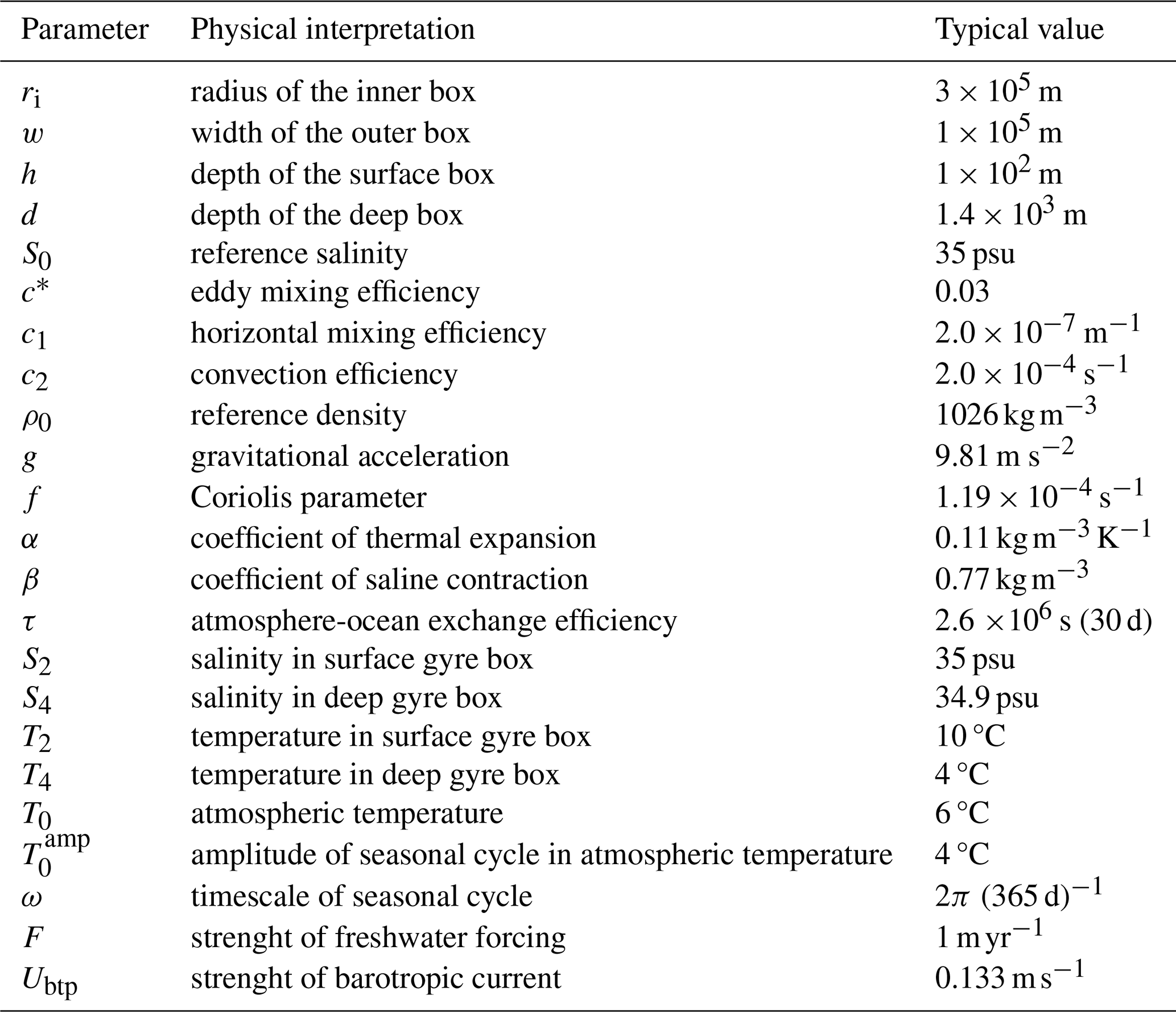
Table A2 Relation between nondimensional and dimensional parameters.

Appendix B: Hopf bifurcations

The presence of Hopf bifurcations at the lower end of the upper branch in a double-fold system (shown more clearly in Fig. B1) is somewhat surprising. The used bifurcation software classified the points eminating from the Hopf bifurcation in the experiments with S₂ as control parameter as supercritical. Although we searched for periodic orbits for both points, we did not find them, possibly because their amplitudes are very small. However, it is not possible to dismiss this bifurcation point as a numerical error. It is found in almost all continuations with S₂ and F as control parameter, and in codim-2 continuations (Fig. 3) the presence of a Hopf point close to the lower saddle node is extremely constant. Since we did not find any periodic orbits in our time integrations, these Hopf bifurcations do not affect the results. No other continuation software was tested for this reason.

It is worth noting that bifurcation analysis of conceptual models describing the AMOC often shows the existence of Hopf bifurcations close to saddle node bifurcations. Titz et al. (2002b) found that when freshwater flux is increased in the four-box interhemispheric model described by Rahmstorf (1996), the upper stable branch loses its stability in a Hopf bifurcation, which is followed by a saddle node linking two unstable branches. It can be shown that this Hopf bifurcation is always subcritical and that as such, all periodic orbits emerging from this point are unstable (Titz et al., 2002a). These results were replicated in the five-box model described in Wood et al. (2019) by Alkhayuon et al. (2019), who also found that the distance between the Hopf and saddle node bifurcations increases with increasing atmospheric CO₂ concentrations. Furthermore, the presence of a subcritical Hopf point near a saddle node is also found in hosing experiments with ESMs (van Westen et al., 2024), indicating that this result is not unique to models of low and intermediate complexity.

Since the Hopf bifurcations do not affect our results, we kept the discussion of these points to a minimum in the main text.

.

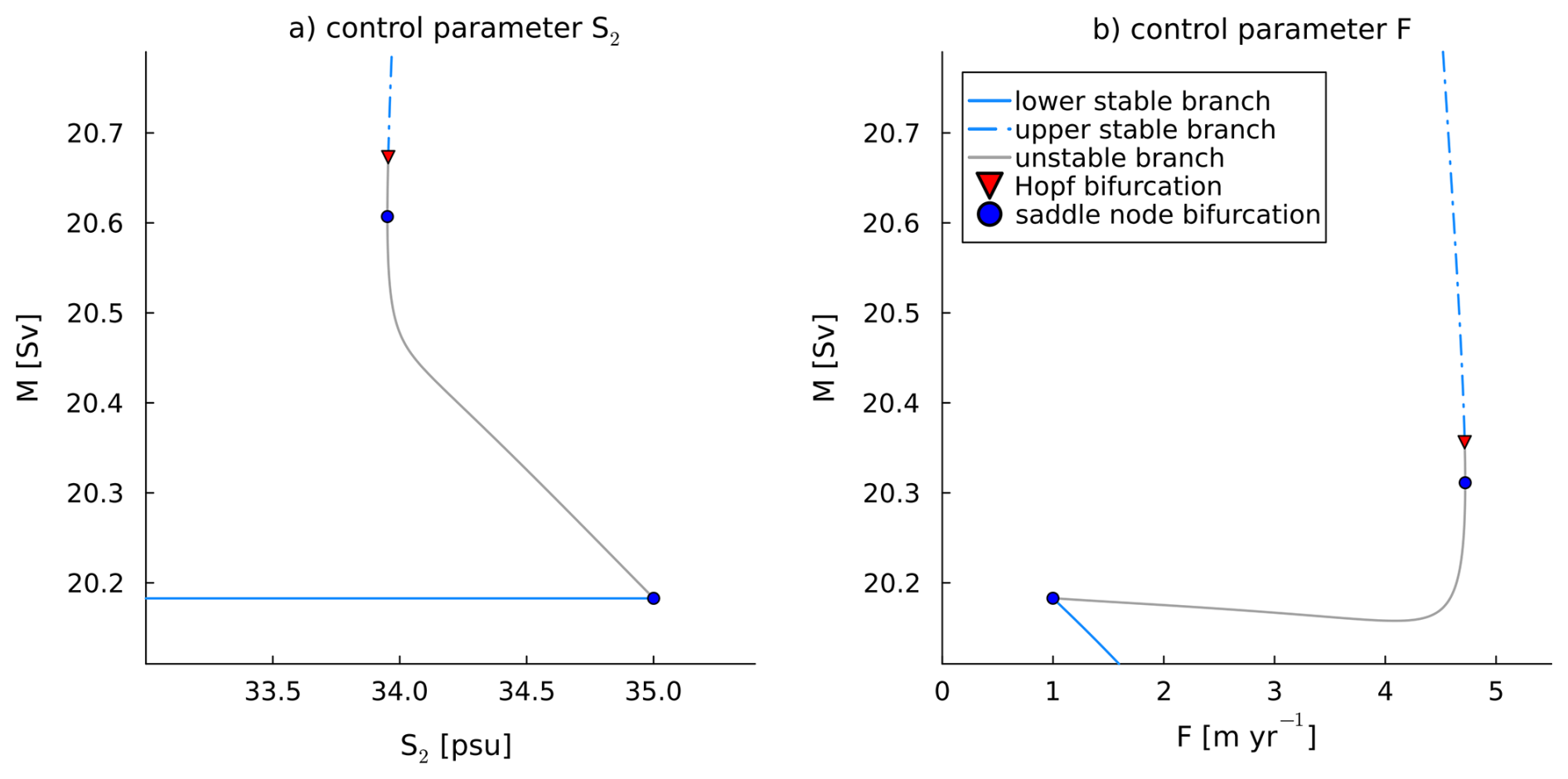
Figure B1 Zoom of Fig. 2 showing the relative location of the stable branches, unstable branches, and Hopf and saddle node bifurcations. The continuation software classified the Hopf bifurcation in subfigure a as supercritical, whereas the one in subfigure b was classified as subcritical. Note the conceptual similarity between subfigure b, Figure 2 in Titz et al. (2002b) and Figs. 3 and 4 Alkhayuon et al. (2019)

Appendix C: Supplementary Figures

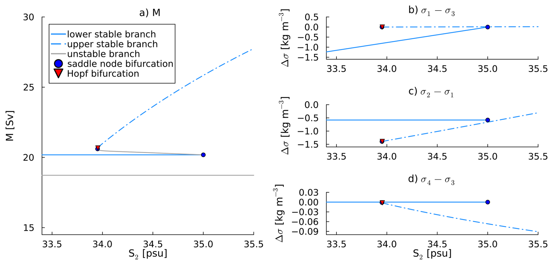
Figure C1 The two stable branches in terms of transport M and horizontal and vertical density differences. Subfigure a: bifurcation diagram with S₂ as control parameter and M on the vertical axis. This is the same result as shown in Fig. 2a. Subfigures (b)–(d): bifurcation diagrams with S₂ as control parameter and vertical (subfigure b) and horizontal surface and deep (subfigures c and d, respectively) density differences on the vertical axis.

Figure C2 Time series and statistics of time integrations of the non-autonomous model with noise level σ_S=0.5 psu. The letters A to F on the left denote the sets of parameter values in (S₂,F)-space, as defined in Fig. 3. Subfigure (a) (d, g, j, m, p): time series of gyre transport M for the last 500 model years. The gyre is considered to be non-convective when M<21 Sv, indicated by grey shading in the time series. Subfigure (b) (e, h, k, n, q): kernel density of the gyre transport M, showing the relative occurence of years with and without convection. Subfigure (c) (f, i, l, o, r): kernel density of time spent in the state with no convection. Note that the y-axis of this right column is scaled differently for every plot. All integrations were performed for 5000 model years. Yearly averaged values were used to calculate the kernel density estimates.