Conditions for instability in the climate–carbon cycle system

The climate and carbon cycle interact in multiple ways. An increase in carbon dioxide in the atmosphere warms the climate through the greenhouse effect, but also leads to uptake of CO₂ by the land and ocean sink, a negative feedback. However, the warming associated with a CO₂ increase is also expected to suppress carbon uptake, a positive feedback. This study addresses the question: “under what circumstances could the climate–carbon cycle system become unstable?” It uses both a reduced form model of the climate–carbon cycle system as well as the complex land model JULES, combined with linear stability theory, to show that: (i) the key destabilising loop involves the increase in soil respiration with temperature; (ii) the climate–carbon system can become unstable if either the climate sensitivity to CO₂ or the sensitivity of soil respiration to temperature is large, and (iii) the climate–carbon system is stabilized by land and ocean carbon sinks that increase with atmospheric CO₂, with CO₂-fertilization of plant photosynthesis playing a key role. For central estimates of key parameters, the critical equilibrium climate sensitivity (ECS) that would lead to instability at current atmospheric CO₂ lies between about 11 K (for large CO₂ fertilization) and 6 K (for no CO₂ fertilization). Given the apparent stability of the climate–carbon cycle, we can view these parameter combinations as implausible. The latter value is close to the highest ECS values amongst the latest Earth Systems Models. Contrary to a previous study that did not include an interactive ocean carbon cycle sink, we find that the stability of the climate–carbon system increases with atmospheric CO₂, such that the glacial CO₂ concentration of 190 ppmv would be unstable even for ECS greater than around 4.5 K in the absence of CO₂ fertilization of land photosynthesis.

1 Introduction

Earth's climate and carbon cycle are intimately coupled. Variations in global mean temperature throughout Earth's history have been linked to changes in atmospheric CO₂ concentrations (Zachos et al., 2001; Judd et al., 2024). The glacial-interglacial cycles that have occurred over the last 800 000 years are associated with ice-sheet dynamics and Milankovitch orbital forcing, but changes in CO₂ concentration have also played a role in significantly amplifying the glacial to interglacial differences (Petit et al., 1999; Marcott et al., 2014).

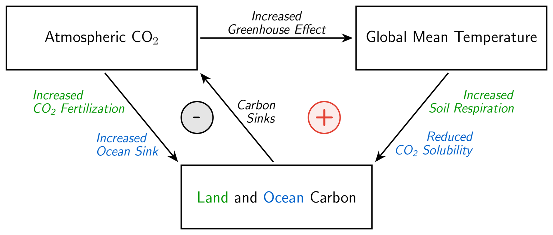
Figure 1 A schematic of the climate–carbon cycle interactions and feedbacks relevant to this study. This shows the negative (stabilising) increased CO₂ leading to increased carbon sink feedback loop, and the positive (destabilising) increased global temperatures leading to a reduced carbon sink feedback loop.

Since the mid-nineteenth century atmospheric CO₂ concentrations have increased by 50 % due to anthropogenic emissions from fossil fuel burning and deforestation, which has driven global warming through an enhanced greenhouse effect (Chen et al., 2021). The carbon cycle has played an important role here, absorbing about half of the anthropogenic emissions of CO₂ through land and ocean carbon sinks (Canadell et al., 2021).

Contemporary land and ocean carbon sinks are the net effect of positive (amplifying) and negative (dampening) feedback loops (see Fig. 1). Increases in atmospheric CO₂ lead to an imbalance between the atmosphere and the surface ocean which results in additional CO₂ being dissolved in seawater and ultimately exported to depth by ocean circulations and marine biota (DeVries, 2022). In the absence of major nutrient limitations, the extra atmospheric CO₂ also increases the photosynthetic rates of land plants, which enables them to store more carbon and create the land carbon sink (Schimel et al., 2015). Both of these effects lead to an increased carbon sink due to increased CO₂. Therefore, they act to dampen an initial CO₂ perturbation (i.e. they are negative feedbacks).

The radiative forcing due to CO₂ leads to increases in global temperatures, which cause predominantly amplifying feedbacks (i.e. positive feedbacks). The positive feedbacks are particularly apparent on the land where the rate of heterotrophic respiration from the soil is known to increase significantly with warming (Davidson and Janssens, 2006; Jenkinson et al., 1991). Enhanced respiration on the land due to CO₂-induced warming is therefore projected to counteract CO₂-fertilization (Friedlingstein et al., 2006, 2014; Arora et al., 2020). In one early model, this increased temperatures leading to a reduced sink effect eventually overwhelmed CO₂ fertilisation of photosynthesis in the mid-21st century, converting the global land carbon sink into a source and significantly accelerating climate change (Cox et al., 2000).

This latter result amounted to a net positive feedback of the carbon cycle on anthropogenic climate change (feedback gain factor, g>0), but it did not lead to an instability or “runaway” (which requires g>1), in which small perturbations to atmospheric carbon grow rapidly. A subsequent analysis explored the conditions that could have led to a runaway climate–carbon cycle feedback (Cox et al., 2006), concluding that this would require at least one of the Equilibrium Climate Sensitivity (ECS) or sensitivity of soil respiration to temperature to be unrealistically high (e.g. respiration increasing by a factor of 6 or more for every 10 K of warming), and that the climate–carbon cycle would become less stable with increases in the CO₂ concentration due to the saturation of CO₂ fertilization at high-CO₂.

In this study we reconsider the potential instability of the coupled climate–carbon system, for two main reasons. Firstly, we note that the upper range of ECS values has increased significantly in the CMIP6 generation of Earth System Models (ESMs), with some models now recording ECS values of up to 6 K (Zelinka et al., 2020). This increases the probability that some ESMs could suffer a climate–carbon cycle instability. Secondly, the Cox et al. (2006) study did not include the important stabilising effect of an interactive ocean carbon cycle, instead assuming that a fixed fraction of any atmospheric CO₂ perturbation would be taken up instantaneously by the ocean.

We use a more sophisticated representation of the ocean carbon cycle, alongside more complete representations of global warming and land carbon feedbacks, to answer the question: “under what circumstances could the climate–carbon cycle system become unstable?”. To do this we perform a bifurcation analysis, which is a analysis of how the stability of a system changes as parameters change, of a conceptual model of the climate–carbon system and find our results are consistent with the output of the complex JULES global land-surface model (Clark et al., 2011; Best et al., 2011).

2 Conceptual model

To investigate the stability of the carbon–climate system, we construct a low dimensional model which represents important climate–carbon processes. We do this by combining existing models of components of the climate–carbon cycle system. This model can be analysed to determine critical parameter values that lead to a bifurcation and can be easily integrated numerically across a range of parameter values to determine its stability.

The model is composed of a climate component which models global temperature anomalies and a carbon cycle component which calculates the fluxes of carbon between the atmosphere, land and ocean. Very slow carbon cycle processes, such as the flux of carbon into and out of the solid Earth, and variations in astronomical forcing are neglected. As a result this model is not valid for longer than millennial timescales.

For the climate component, we use a two-box energy balance model. One box represents the globally averaged temperature anomaly of the atmosphere and upper ocean, T₁ (units of K), and the other represents the globally averaged temperature anomaly of the deep ocean, T₂ (K).

Radiative forcing due to a CO₂ increase heats the upper box, with a forcing due to each CO₂ doubling of Q_2× (Myhre et al., 1998). This logarithmic dependence means that each additional unit of CO₂ added to the atmosphere has a weaker effect than the previous.

The boxes exchange energy with each other, parametrised by a heat transfer coefficient κ, and respond to the radiative forcing caused by CO₂, which follows the standard logarithmic form. This type of model can be fitted to the outputs of more complex Earth System Models (Cummins et al., 2020; Williamson et al., 2024) and has been shown to accurately reproduce the response to radiative forcing (Geoffroy et al., 2013).

The terrestrial carbon store, C_L (Pg C), is modelled by the balance between globally averaged Net Primary Production (NPP), denoted by Π, and globally averaged heterotrophic respiration. We will neglect to explicitly represent vegetation dynamics on the assumption that the timescales of interest for the stability of the system are longer than typical vegetation timescales.

NPP is assumed to be a function of atmospheric CO₂ only. The temperature dependence of NPP is neglected, as the temperature response is weaker, at the global scale, than the CO₂ response (Varney et al., 2023). To model heterotrophic respiration we make the common assumption that it follows a Q₁₀ response formula, in which respiration increases by a factor of Q₁₀ for every 10 K warming. We also assume that the relevant temperature for heterotrophic respiration is the temperature over land, which is larger than global temperatures by a factor β≈1.3 (Byrne and O'Gorman, 2018).

Ocean carbon uptake is represented with a two box model developed by Bolin and Eriksson (1959) and Glotter et al. (2014). The boxes represent the upper and deep ocean carbon stores C₁ and C₂ (Pg C), respectively, these boxes do not partition the ocean into the same way the temperature boxes do. This model accounts for changes in ocean chemistry due to increased ocean carbon. However, following Glotter et al. (2014), we neglect the role of temperature change in carbon uptake, as this effect is smaller than the direct effect of increased CO₂ concentrations (Arora et al., 2020).

Atmospheric carbon, C_A, is required to close the model. C_A is calculated by applying conservation of mass to the total carbon in the system. Mathematically, the model can be written as:

$$\begin{array}{}\text{(1a)}& {\displaystyle }{c}_{\mathrm{1}}{\displaystyle \frac{\mathrm{d}{T}_{\mathrm{1}}}{\mathrm{d}t}}& {\displaystyle }=-\mathit{\lambda }{T}_{\mathrm{1}}+\mathit{\kappa }(T_{\mathrm{2}}-T_{\mathrm{1}})+Q_{\mathrm{2}\times }{\log }_{\mathrm{2}}\left({\displaystyle \frac{C_{\mathrm{A}}}{C_{\mathrm{A}}^{\ast }}}\right)\text{(1b)}& {\displaystyle }{c}_{\mathrm{2}}{\displaystyle \frac{\mathrm{d}{T}_{\mathrm{2}}}{\mathrm{d}t}}& {\displaystyle }=-\mathit{\kappa }(T_{\mathrm{2}}-T_{\mathrm{1}})\text{(1c)}& {\displaystyle \frac{\mathrm{d}{C}_{\mathrm{L}}}{\mathrm{d}t}}& {\displaystyle }=\mathrm{\Pi }\left(C_{\mathrm{A}}\right)-\mathrm{\Pi }\left(C_{\mathrm{A}}^{\ast }\right){\displaystyle \frac{C_{\mathrm{L}}}{C_{\mathrm{L}}^{\ast }}}{e}^{\mathit{\alpha }\mathit{\beta }{T}_{\mathrm{1}}}\text{(1d)}& {\displaystyle \frac{\mathrm{d}{C}_{\mathrm{1}}}{\mathrm{d}t}}& {\displaystyle }={\mathit{\nu }}_{\mathrm{1}}(C_{\mathrm{A}}-\mathcal{E}(C_{\mathrm{1}}\left)\right)-{\mathit{\nu }}_{\mathrm{2}}\left(C_{\mathrm{1}}-{\displaystyle \frac{V_{\mathrm{1}}}{V_{\mathrm{2}}}}{C}_{\mathrm{2}}\right)\text{(1e)}& {\displaystyle \frac{\mathrm{d}{C}_{\mathrm{2}}}{\mathrm{d}t}}& {\displaystyle }={\mathit{\nu }}_{\mathrm{2}}\left(C_{\mathrm{1}}-{\displaystyle \frac{V_{\mathrm{1}}}{V_{\mathrm{2}}}}{C}_{\mathrm{2}}\right),\end{array}$$

with carbon conservation giving

$$\begin{array}{}\text{(2)}& C_{\mathrm{A}}+C_{\mathrm{L}}+C_{\mathrm{1}}+C_{\mathrm{2}}=C_{\mathrm{A}}^{\ast }+C_{\mathrm{L}}^{\ast }+C_{\mathrm{1}}^{\ast }+C_{\mathrm{2}}^{\ast },\end{array}$$

where asterisks indicate pre-industrial values.

The parameters c₁ and c₂ denote the different heat capacities of the two climate boxes. Furthermore, rather than working with ECS directly, we introduce a climate feedback parameter λ, which is related to ECS by the formula $\text{ECS}=Q_{\mathrm{2}\times }/\mathit{\lambda }$.

The parameter α determines the strength of heterotrophic respiration and is related to Q₁₀ by α=0.1log Q₁₀. The exact form of Π is not important for analytical results, as the linear stability of the pre-industrial equilibrium will only depend on $\mathrm{\Pi }\left(C_{\mathrm{A}}^{\ast }\right)$ and its derivative ${\mathrm{\Pi }}^{\prime }\left(C_{\mathrm{A}}^{\ast }\right)$. However for numerical experiments, we assume the saturating form

$$\begin{array}{}\text{(3)}& \mathrm{\Pi }\left(C_{\mathrm{A}}\right)=\mathrm{\Pi }\left(C_{\mathrm{A}}^{\ast }\right){\displaystyle \frac{C_{\mathrm{A}}^{\ast }+C_{\mathrm{1}/\mathrm{2}}}{C_{\mathrm{A}}^{\ast }}}{\displaystyle \frac{C_{\mathrm{A}}}{C_{\mathrm{A}}+C_{\mathrm{1}/\mathrm{2}}}}\end{array}$$

where $C_{\mathrm{1}/\mathrm{2}}$ is a half-saturation constant.

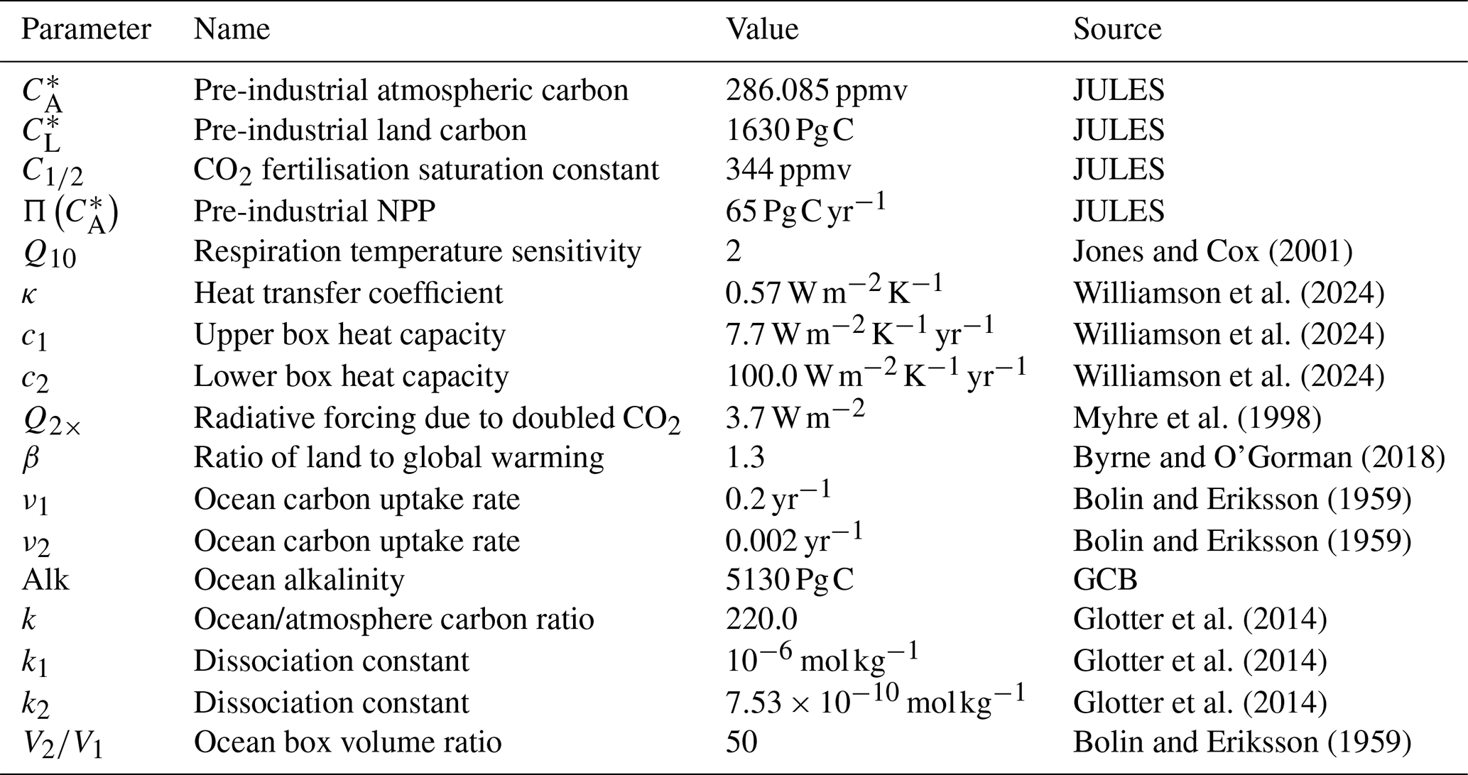
Jones and Cox (2001)Williamson et al. (2024)Williamson et al. (2024)Williamson et al. (2024)Myhre et al. (1998)Byrne and O'Gorman (2018)Bolin and Eriksson (1959)Bolin and Eriksson (1959)Glotter et al. (2014)Glotter et al. (2014)Glotter et al. (2014)Bolin and Eriksson (1959)

Table 1 The “default” parameter values used for the numerical evaluation of the model, unless otherwise stated. No default value is given for λ as that parameter is changed throughout the study.

The upper ocean box, with volume V₁, absorbs carbon from the atmosphere over a fast timescale  ${\mathit{\nu }}_{\mathrm{1}}^{-\mathrm{1}}$. This carbon is transported to the larger lower box, with volume V₂, on a slower timescale, ${\mathit{\nu }}_{\mathrm{2}}^{-\mathrm{1}}$. These timescale parameters capture the effects of carbon pumps, which transport carbon to depth. We account for the effects of ocean chemistry with the function ℰ, which relates C₁ to the amount of atmospheric carbon required for equilibrium. The functional form of ℰ can be derived by assuming constant alkalinity, Alk, in the ocean. Here Alk represents carbonate alkalinity, not total alkalinity. We note that this assumption leads to lower ocean pH values than more sophisticated methods (Munhoven, 2013). The expression for ℰ is

$$\begin{array}{}\text{(4)}& \mathcal{E}\left(C_{\mathrm{1}}\right)=k{\left(\mathrm{1}+{\displaystyle \frac{k_{\mathrm{1}}}{\left[{\mathrm{H}}^{+}\right]}}+{\displaystyle \frac{k_{\mathrm{1}}{k}_{\mathrm{2}}}{[{\mathrm{H}}^{+}{]}^{\mathrm{2}}}}\right)}^{-\mathrm{1}}{C}_{\mathrm{1}}\end{array}$$

where the concentration of hydrogen ions, [H⁺], can be found by solving

$$\begin{array}{}\text{(5)}& \text{Alk}=\left({\displaystyle \frac{k_{\mathrm{1}}}{\left[{\mathrm{H}}^{+}\right]}}+{\displaystyle \frac{\mathrm{2}{k}_{\mathrm{1}}{k}_{\mathrm{2}}}{[{\mathrm{H}}^{+}{]}^{\mathrm{2}}}}\right){\left(\mathrm{1}+{\displaystyle \frac{k_{\mathrm{1}}}{\left[{\mathrm{H}}^{+}\right]}}+{\displaystyle \frac{k_{\mathrm{1}}{k}_{\mathrm{2}}}{[{\mathrm{H}}^{+}{]}^{\mathrm{2}}}}\right)}^{-\mathrm{1}}{C}_{\mathrm{1}}.\end{array}$$

The total amount of carbon in the system can be written as the sum of $C_{\mathrm{L}}^{\ast }$, $C_{\mathrm{1}}^{\ast }$, $C_{\mathrm{2}}^{\ast }$, $C_{\mathrm{A}}^{\ast }$ which are the pre-industrial carbon stores in the land, upper ocean, deep ocean and atmospheric reservoirs, respectively. Whilst $C_{\mathrm{L}}^{\ast }$ and $C_{\mathrm{A}}^{\ast }$ are free parameters of the model, the pre-industrial ocean values are calculated from the equations $C_{\mathrm{A}}^{\ast }=\mathcal{E}\left(C_{\mathrm{1}}^{\ast }\right)$ and $C_{\mathrm{2}}^{\ast }=(V_{\mathrm{2}}/V_{\mathrm{1}})C_{\mathrm{1}}^{\ast }$.

2.1 Parameters

The parameters take the values given in Table 1, unless otherwise stated. These values mostly come from previous estimates in the literature, however some come from the output of a complex terrestrial carbon cycle model, JULES. The only parameter that we have fitted ourselves is the Alk parameter, which was chosen so that the ocean model correctly estimates the observed ocean carbon uptake over the historical period, inferred by the Global Carbon Budget (GCB) (Friedlingstein et al., 2022) (see Fig. S1 in the Supplement). We fit to the ocean uptake rather than the total ocean carbon as the response to elevated CO₂ plays an important role in the system's stability. As our ocean carbon model has only two boxes, it is not suitable to accurately simulate the size of the total ocean carbon store on multi-millennial timescales.

2.2 Analysis

The pre-industrial state is an equilibrium of Eq. (1), occurring when $T_{\mathrm{1}}=T_{\mathrm{2}}=\mathrm{0}$, $C_{\mathrm{A}}=C_{\mathrm{A}}^{\ast }$, $C_{\mathrm{L}}=C_{\mathrm{L}}^{\ast }$, $C_{\mathrm{1}}=C_{\mathrm{1}}^{\ast }$ and $C_{\mathrm{2}}=C_{\mathrm{2}}^{\ast }$. Furthermore, this equilibrium exists for all parameter values.

To calculate the stability of this pre-industrial equilibrium it is helpful to rewrite Eq. (1) in the condensed form

$$\begin{array}{}\text{(6)}& {\displaystyle \frac{\mathrm{d}\mathit{x}}{\mathrm{d}t}}=\mathit{f}\left(\mathit{x}\right)\end{array}$$

where $\mathit{x}=(T_{\mathrm{1}},T_{\mathrm{2}},C_{\mathrm{L}},C_{\mathrm{1}},C_{\mathrm{2}}{)}^{\mathrm{T}}$ and f is given by the right-hand side of Eq. (1). Letting x^∗ be the pre-industrial equilibrium, we can linearise Eq. (6) about x^∗ to give the behaviour of small perturbations Δx

$$\begin{array}{}\text{(7)}& {\displaystyle \frac{\mathrm{d}\mathbf{\Delta }\mathit{x}}{\mathrm{d}t}}=\mathbf{J}\mathbf{\Delta }\mathit{x}\end{array}$$

where the Jacobian, J, is given by ${\mathbf{J}}_{ij}=\partial {\mathit{f}}_i/\partial {\mathit{x}}_j$ evaluated at x^∗.

At large t, the perturbation will be dominated by a contribution along the fastest growing (or slowest decaying) direction in phase space, which is the space of possible states of the system. Mathematically, as t→∞, the perturbation behaves like Δx(t)∼c_mv_mexp (γ_mt) where γ_m is the eigenvalue of J with the largest real part, v_m the corresponding eigenvector and c_m a constant given by the initial conditions. If Reγ_m>0, the perturbation grows and therefore the equilibrium is unstable. If Reγ_m<0 the perturbation decays and so the equilibrium is stable.

Therefore we must determine when the eigenvalues of J have zero real part to find the critical parameters for which the stability of the pre-industrial equilibrium changes. Evaluated at the pre-industrial equilibrium, J is

$$\begin{array}{}\text{(8)}& \mathbf{J}=\left[\begin{array}{ccccc}-{\displaystyle \frac{\mathit{\lambda }+\mathit{\kappa }}{c_{\mathrm{1}}}}& \frac{\mathit{\kappa }}{c_{\mathrm{1}}}& -\frac{Q_{\mathrm{2}\times }}{c_{\mathrm{1}}{C}_{\mathrm{A}}^{\ast }\log \mathrm{2}}& -\frac{Q_{\mathrm{2}\times }}{c_{\mathrm{1}}{C}_{\mathrm{A}}^{\ast }\log \mathrm{2}}& -\frac{Q_{\mathrm{2}\times }}{c_{\mathrm{1}}{C}_{\mathrm{A}}^{\ast }\log \mathrm{2}}\\ \frac{\mathit{\kappa }}{c_{\mathrm{2}}}& -\frac{\mathit{\kappa }}{c_{\mathrm{2}}}& \mathrm{0}& \mathrm{0}& \mathrm{0}\\ -\mathit{\alpha }\mathit{\beta }\mathrm{\Pi }\left(C_{\mathrm{A}}^{\ast }\right)& \mathrm{0}& -\frac{\mathrm{d}\mathrm{\Pi }}{\mathrm{d}{C}_{\mathrm{A}}}-\frac{\mathrm{\Pi }\left(C_{\mathrm{A}}^{\ast }\right)}{C_{\mathrm{L}}^{\ast }}& -\frac{\mathrm{d}\mathrm{\Pi }}{\mathrm{d}{C}_{\mathrm{A}}}& -\frac{\mathrm{d}\mathrm{\Pi }}{\mathrm{d}{C}_{\mathrm{A}}}\\ \mathrm{0}& \mathrm{0}& -{\mathit{\nu }}_{\mathrm{1}}& -{\mathit{\nu }}_{\mathrm{1}}\left(\mathrm{1}+{\mathcal{E}}^{\prime }\left(C_{\mathrm{1}}^{\ast }\right)\right)-{\mathit{\nu }}_{\mathrm{2}}& -{\mathit{\nu }}_{\mathrm{1}}+\frac{V_{\mathrm{1}}}{V_{\mathrm{2}}}{\mathit{\nu }}_{\mathrm{2}}\\ \mathrm{0}& \mathrm{0}& \mathrm{0}& {\mathit{\nu }}_{\mathrm{2}}& -\frac{V_{\mathrm{1}}}{V_{\mathrm{2}}}{\mathit{\nu }}_{\mathrm{2}}\end{array}\right]\end{array}$$

where ℰ^′ denotes the derivative of ℰ with respect to C₁. The eigenvalues, γ, of the Jacobian satisfy the characteristic equation, $\text{det}(\mathbf{J}-\mathit{\gamma }\mathrm{I})=\mathrm{0}$ giving

$$\begin{array}{}\text{(9)}& {\mathit{\gamma }}^{\mathrm{5}}+p_{\mathrm{4}}{\mathit{\gamma }}^{\mathrm{4}}+p_{\mathrm{3}}{\mathit{\gamma }}^{\mathrm{3}}+p_{\mathrm{2}}{\mathit{\gamma }}^{\mathrm{2}}+p_{\mathrm{1}}\mathit{\gamma }+p_{\mathrm{0}}=\mathrm{0},\end{array}$$

where {p_i} are functions of the parameters of the model.

Ideally, we would solve Eq. (9) for γ and would then find the critical parameter values for which Reγ=0. However, because Eq. (9) is a quintic polynomial, no general solution exists. Therefore, we must rely on special cases and approximations to make progress.

A simple case occurs when γ is purely real. In that case, γ=0 is a solution when p₀=0. When p₀=0, The parameters satisfy

$$\begin{array}{}\text{(10)}& {\displaystyle \frac{\mathit{\alpha }\mathit{\beta }{Q}_{\mathrm{2}\times }}{\mathit{\lambda }\log \mathrm{2}}}={\displaystyle \frac{V_{\mathrm{2}}}{V_{\mathrm{1}}}}{\displaystyle \frac{\mathrm{d}\log \mathrm{\Pi }}{\mathrm{d}\log C_{\mathrm{A}}}}+{\displaystyle \frac{C_{\mathrm{A}}^{\ast }}{C_{\mathrm{L}}^{\ast }}}\left(\mathrm{1}+{\displaystyle \frac{\mathrm{1}}{{\mathcal{E}}^{\prime }}}+{\displaystyle \frac{\mathrm{1}}{{\mathcal{E}}^{\prime }}}{\displaystyle \frac{V_{\mathrm{2}}}{V_{\mathrm{1}}}}\right).\end{array}$$

The bifurcation this corresponds to can be shown to be a transcritical bifurcation, in which a new stable steady state emerges near to the old, now unstable, steady state.

If γ has non-zero imaginary part, exact results cannot be obtained. However, because we are interested in γ values near the bifurcation, we can guarantee that Reγ is small. Making the further assumption that Imγ is small means that cubic terms and higher can be dropped from Eq. (9). The resulting quadratic equation can be solved to give

$$\begin{array}{}\text{(11)}& \mathrm{Re}\mathit{\gamma }\approx -{\displaystyle \frac{p_{\mathrm{1}}}{\mathrm{2}{p}_{\mathrm{2}}}},\end{array}$$

which in terms of the climate feedback parameter, λ, can be written as

$$\begin{array}{}\text{(12)}& \mathrm{Re}\mathit{\gamma }\approx {\displaystyle \frac{\mathit{\lambda }+g_{\mathrm{1}}}{g_{\mathrm{2}}\mathit{\lambda }+g_{\mathrm{3}}}},\end{array}$$

where {g_i} are functions of the parameters.

Setting this growth rate equal to zero gives an expression for the critical λ, which is given in the Supplement as Eq. (S1). The resulting equation is too complicated to be useful; however further approximations can be made to make it tractable. As the deep ocean is much larger and absorbs carbon over a slower timescale than the upper ocean, it can be assumed that ${\mathcal{E}}^{\prime }{\mathit{\nu }}_{\mathrm{1}}\gg {\mathit{\nu }}_{\mathrm{2}}$, ν₁≫ν₂, c₂≫c₁ and V₂≫V₁. In this approximation, the equation reduces to

$$\begin{array}{}\text{(13)}& \begin{array}{rl}{\displaystyle \frac{\mathit{\alpha }\mathit{\beta }{Q}_{\mathrm{2}\times }}{\mathit{\lambda }\log \mathrm{2}}}=& \left({\displaystyle \frac{\mathrm{d}\log \mathrm{\Pi }}{\mathrm{d}\log C_{\mathrm{A}}}}+{\displaystyle \frac{C_{\mathrm{A}}^{\ast }}{C_{\mathrm{L}}^{\ast }}}\left(\mathrm{1}+{\displaystyle \frac{\mathrm{1}}{{\mathcal{E}}^{\prime }}}+{\displaystyle \frac{c_{\mathrm{2}}{\mathit{\nu }}_{\mathrm{2}}}{\mathit{\kappa }{\mathcal{E}}^{\prime }}}+{\displaystyle \frac{C_{\mathrm{L}}^{\ast }{\mathit{\nu }}_{\mathrm{2}}}{{\mathrm{\Pi }}_{\mathrm{0}}{\mathcal{E}}^{\prime }}}\right)\right)\\ & \times \left(\mathrm{1}+{\displaystyle \frac{C_{\mathrm{A}}^{\ast }{\mathit{\nu }}_{\mathrm{2}}{c}_{\mathrm{2}}}{C_{\mathrm{L}}^{\ast }{\mathcal{E}}^{\prime }\mathit{\alpha }\mathit{\beta }{Q}_{\mathrm{2}\times }}}\right).\end{array}\end{array}$$

As γ is purely imaginary, this corresponds to a Hopf bifurcation, which means the system transitions from a steady state to an oscillatory state.

It  should be noted that Eq. (10) contains factors of $V_{\mathrm{2}}/V_{\mathrm{1}}$ whereas Eq. (13) does not. The deep ocean is much larger than the upper ocean, V₂≫V₁. This means that the transcritical bifurcation occurs at much higher values of ECS than the Hopf bifurcation does. Therefore, we will focus on the Hopf bifurcation in the rest of the study.

The approximate expression for the critical climate sensitivity, Eq. (13), was verified by numerically calculating the growth rate from the Jacobian, J, and identifying where it is zero. This numerical result was compared to Eq. (13) for a range of ECS and CO₂ fertilisation strengths, and for three different $C_{\mathrm{A}}^{\ast }$ values. Although $C_{\mathrm{A}}^{\ast }$ was introduced as the amount of carbon stored in the pre-industrial atmosphere, we can generalise this to the case where $C_{\mathrm{A}}^{\ast }$ represents a potential atmospheric carbon steady state, and measure temperature anomalies relative to the global temperatures the value of $C_{\mathrm{A}}^{\ast }$ implies. We can then determine how stable or unstable that state would be. This allows us to consider how the amount of carbon in the atmosphere affects the stability of the system. These $C_{\mathrm{A}}^{\ast }$ values correspond to the pre-industrial equilibrium, a doubling of CO₂ and $C_{\mathrm{A}}^{\ast }=\mathrm{190}$ppmv which was the atmospheric CO₂ level during at Last Glacial Maximum (LGM) (Kageyama et al., 2017).

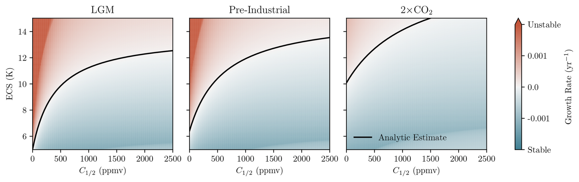
Figure 2 Growth rates of perturbations to the equilibrium state in the conceptual model, Eq. (1), for a range of ECS, CO₂ fertilisation effect strengths, and different atmospheric carbon levels. The colours correspond to growth rates calculated numerically and the solid line is given by Eq. (13). This line agrees with the numerics as to when the growth rate is zero.

The results are shown in Fig. 2. The figure shows the numerically determined growth rates, as well as the approximation Eq. (13). The approximation gives good agreement with the numerically determined values, supporting the usefulness of the approximation Eq. (13) across a range of parameter values.

It is worth dwelling on the meaning of the individual terms in Eq. (13). The left-hand side of the equation consists of a product of two sensitivities. One sensitivity in the product is $Q_{\mathrm{2}\times }/\mathit{\lambda }=\text{ECS}$, which is the sensitivity of global temperatures to atmospheric carbon. The other sensitivity is the sensitivity of respiration to increased land temperatures, αβ. These are the two ingredients in the positive feedback loop between global temperatures and respiration. The two factors do not enter Eq. (13) on totally equal terms, however, as a factor of αβ also appears on the right-hand side of the equation.

The right-hand side of Eq. (13) consists of negative feedbacks which stabilise the climate–carbon system. The first of these is $\mathrm{d}\log \mathrm{\Pi }/\mathrm{d}\log C_{\mathrm{A}}$, which measures the magnitude of the CO₂ fertilisation effect. The larger this is, the more stable the system becomes. The next term is a factor in parentheses multiplied by the ratio $C_{\mathrm{A}}^{\ast }/C_{\mathrm{L}}^{\ast }$. This ratio implies that the greater the proportion of carbon held in the atmosphere relative to land the more stable the system is. This effect can be attributed to the fact that heterotrophic respiration increases linearly with land carbon but radiative forcing increases only logarithmically with CO₂. As it is the ratio, rather than the sum, of carbon stored in the atmosphere to carbon stored in the land that appears in Eq. (13), the stability of the system does not depend straightforwardly on the total carbon store.

The factor in parentheses is a sum of timescale ratios. The timescales are: $\mathit{\kappa }/c_{\mathrm{2}}$ (ocean heat uptake timescale), ${\mathit{\nu }}_{\mathrm{2}}^{-\mathrm{1}}$ (deep ocean carbon uptake timescale) and $C_{\mathrm{L}}^{\ast }/{\mathrm{\Pi }}_{\mathrm{0}}$ (soil carbon turnover time). They imply that the system is less stable if the ocean absorbs carbon slowly relative to the time the ocean takes to warm or if carbon cycles quickly through the soil compared to the ocean. Each of these timescale ratios is multiplied by ${\mathcal{E}}^{\prime -\mathrm{1}}$, which describes how a change in ocean carbon affects the air-sea carbon equilibrium. If this value is large, the ocean absorbs more carbon for a given change in atmospheric concentration, which acts to stabilise the system.

2.3 Numerical results

We performed numerical experiments to analyse the behaviour of the model around the bifurcation. We initialised the system near the pre-industrial equilibrium by increasing atmospheric carbon by 20 ppmv and integrating for 50 000 years. This is a longer timescales than the model is strictly valid for, however it gives enough time to show the system's dynamics.

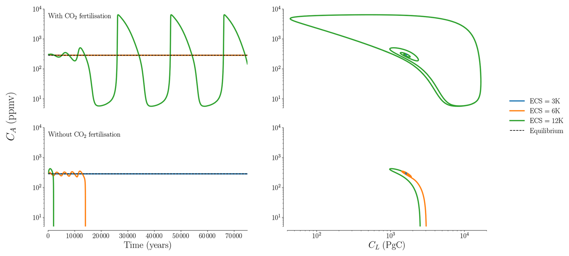
Figure 3 The response of Eq. (1) to a small 20 ppmv perturbation to CO₂ when the ECS is 3, 6 or 12 K and the CO₂ fertilisation effect is either present (top row, $C_{\mathrm{1}/\mathrm{2}}$ = 344 ppmv) or absent (bottom row, $C_{\mathrm{1}/\mathrm{2}}$ = 0 ppmv). The left column shows a time series of atmospheric carbon and the right shows the trajectories projected onto the C_A-C_L plane.

Figure 3 shows the resulting atmospheric CO₂ time series for ECS values of 3, 6 and 12 K. Additionally, we repeated the experiment in the case when the CO₂ fertilisation effect was absent. When the CO₂ effect was present, the cases where the ECS was 3 or 6 K relaxed back to equilibrium; these parameters correspond to a stable equilibrium. However, for an ECS of 12 K the system approaches a limit cycle. Between these ECS values the system passed through a Hopf bifurcation, causing the pre-industrial state to become unstable.

A projection of the C_A-C_L plane is shown in Fig. 3. It shows that the limit cycle involves moving large quantities of carbon between the land and the atmosphere. It should be noted that the amplitude and period of this limit cycle are large enough that the system has been pushed into a regime where the assumptions in the model are no longer strictly valid.

The limit cycle emerges because carbon is transferred back and forth between the land and the atmosphere. When there are sufficient stocks of terrestrial carbon, the positive feedback between heterotrophic respiration and global warming moves carbon from the land to the atmosphere. As there is now less carbon in the land, heterotrophic respiration decreases and, due to the CO₂ fertilisation effect, NPP increases. This means that carbon now instead flows back into the land from the atmosphere, and so the cycle can begin again.

The result of turning off the CO₂ fertilisation effect (i.e. setting $C_{\mathrm{1}/\mathrm{2}}$ to zero) is shown in the bottom row of Fig. 3. In this case, the pre-industrial state becomes unstable at lower values of ECS. In particular instability occurs for an ECS of 6 K. Furthermore, the instability is more serious in that the system diverges rather than approaches a limit cycle. This represents a deficiency the model, arising from not accounting for effects that occur at low CO₂.

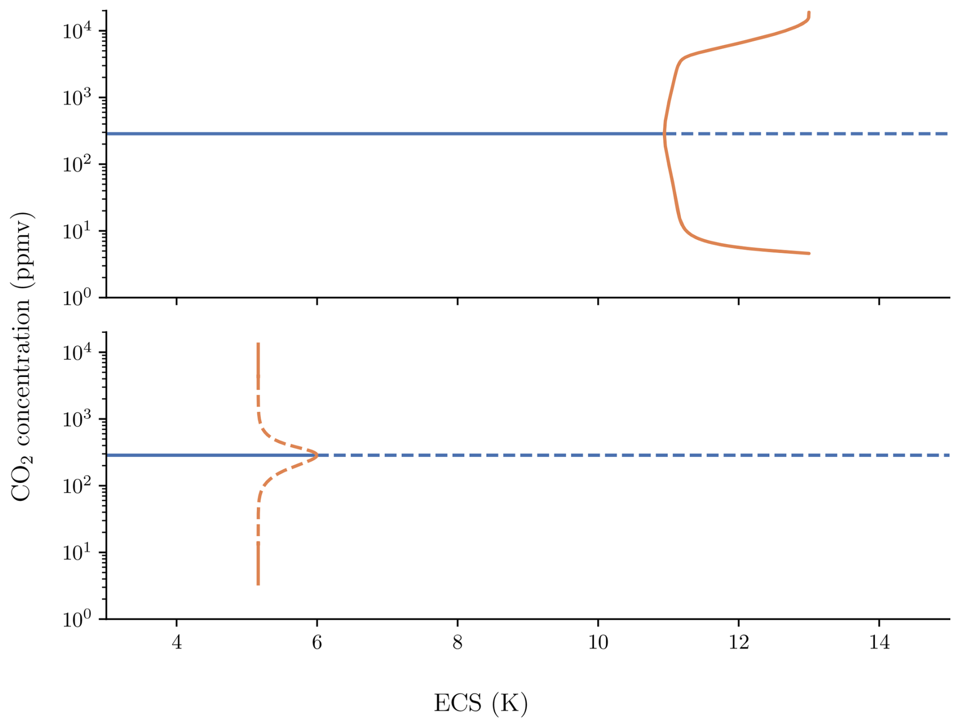
Figure 4 A bifurcation diagram for Eq. (1), showing the equilibrium behaviour of atmospheric carbon as a function of climate sensitivity with a CO₂ fertilisation effect (top) and without (bottom). The blue solid line indicates a stable fixed point, corresponding to the pre-industrial state. The dashed line indicates an unstable fixed point and the orange curves show the maximum and minimum values of the limit cycle.

A more systematic investigation of the system's behaviour can be performed by plotting the system's equilibrium state against a varying parameter, known as a bifurcation diagram. Figure 4 shows a bifurcation diagram of atmospheric carbon as a function of ECS for the cases with and without a CO₂ fertilisation effect, computed by the XPP-AUTO continuation software (Ermentrout, 2002). Figure 4 shows that, with a CO₂ fertilisation effect, above a critical climate sensitivity of 10.9 K, the pre-industrial state is unstable. Beyond this threshold, the system undergoes a Hopf bifurcation and develops large oscillations in the CO₂ levels. When the CO₂ fertilisation effect is absent, the bifurcation occurs at a lower ECS of just below 6 K. The Hopf bifurcation is supercritical (a stable oscillation exists after the bifurcation) in the first case but subcritical (an unstable oscillation exists before the bifurcation) in the second case. This explains why the system diverged in some of the numerical experiments plotted in Fig. 3.

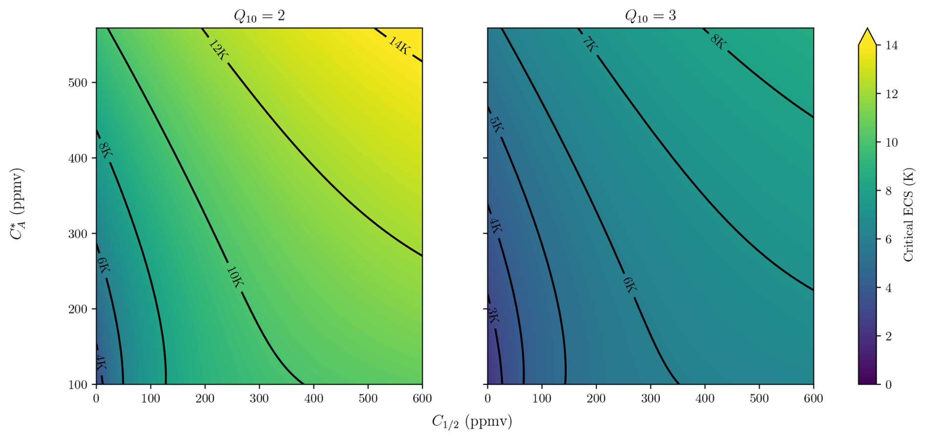
Figure 5 The critical ECS as a function of CO₂ levels, $C_{\mathrm{A}}^{\ast }$, and the CO₂ fertilisation effect for two different values of Q₁₀. Notice the critical ECS is smaller for smaller pre-industrial CO₂ levels, CO₂ fertilisation strength and larger Q₁₀.

The dependence on the CO₂ fertilisation effect strength and pre-industrial CO₂ levels were further investigated, by numerically solving for the eigenvalues of the Jacobian, which are the solutions to Eq. (9). Figure 5 shows the dependence of the critical ECS value on $C_{\mathrm{1}/\mathrm{2}}$ and $C_{\mathrm{A}}^{\ast }$ for Q₁₀=2 and Q₁₀=3. As $C_{\mathrm{A}}^{\ast }$ increases, the critical ECS does too. This indicates that the system is more stable at high CO₂ levels and therefore anthropogenic CO₂ emissions are unlikely to trigger this instability. Furthermore as the strength of the CO₂ fertilisation effect decreases, the system is unstable at lower ECS values.

When Q₁₀=2, Fig. 5 shows that the critical ECS enters the range of CMIP6 models (i.e. less than 6 K) for weak CO₂ fertilisation effects and low CO₂ levels, a regime relevant to the Last Glacial Maximum. If Q₁₀=3 then the critical ECS becomes comparable to the ECS of CMIP6 models, even for a comparatively strong CO₂ fertilisation effect at low enough CO₂ levels.

3 Complex model

Equation (1) is, by construction, a significant simplification of the real Earth system, which has many more processes and is spatially heterogeneous. This is important, for example, as warming caused by increased atmospheric CO₂ is also spatially heterogeneous; the poles warm faster than equatorial regions (Huntingford and Mercado, 2016). To avoid the limitations of the simple model, we examine the results from a complex land surface model, the Joint UK Land Environmental Simulator (JULES) (Best et al., 2011; Clark et al., 2011).

3.1 Model description

JULES is a state-of-the-art model of land-atmosphere exchanges of momentum, water and vapour, and fluxes of carbon. JULES has a dynamic vegetation component (TRIFFID) and a RothC four-pool model of soil carbon, operating at a spatial resolution of 2.5° × 3.75°. JULES is driven by meteorological forcings from a model called the Integrated Model Of Global Effects of climatic aNomalies (IMOGEN), which includes carbon cycle feedbacks on atmospheric and ocean carbon.

IMOGEN is a spatially-explicit intermediate complexity model (Huntingford et al., 2010) which is coupled to the JULES land surface model at the same spatial resolution. IMOGEN provides spatially-explicit meteorological forcings to drive JULES and dynamically responds to changes in CO₂. The response to CO₂ is estimated using pattern scaling, which assumes that the change in some spatially-resolved meteorological variable ΔX at location r, year t, and month m can be written as $\mathrm{\Delta }X(r,t,m)=p(r,m)\stackrel{\mathrm{‾}}{\mathrm{\Delta }T}\left(t\right)$ where p is a spatial pattern and $\stackrel{\mathrm{‾}}{\mathrm{\Delta }T}$ is global mean temperature change. The temperature change is determined by an energy balance model with ocean heat uptake parametrised diffusively. The pattern and energy balance model parameters are fitted to the actual patterns of change projected by different ESMs. In this way, IMOGEN can emulate different ESMs (Huntingford et al., 2000). In this study, we use IMOGEN to create an emulator of the HadGEM2-ES model (Jones et al., 2011).

To close the global carbon cycle, IMOGEN also provides a model for ocean carbon uptake based on the impulse-response formulation given by Joos et al. (1996), which was calibrated to match the behaviour of process-based models. Uptake of carbon by the oceans in IMOGEN depends both on ocean temperatures and atmospheric CO₂ concentrations.

JULES and IMOGEN are fully coupled. IMOGEN provides JULES with meteorological forcing, which affects the terrestrial carbon cycle modelled by JULES. JULES then provides land-atmosphere carbon fluxes to IMOGEN, as the terrestrial land stores evolve. IMOGEN combines this flux with the ocean-atmosphere carbon flux to update atmospheric CO₂, which leads to changes in climate and thus feeds back to the meteorological forcing given to JULES.

3.2 Experimental configuration

For this study, we took advantage of the fact that the ECS of IMOGEN can be set explicitly. This means that we can run multiple experiments varying the ECS values to determine which value of ECS leads to an instability of the pre-industrial state.

To initialise JULES in a pre-industrial equilibrium state, the JULES/IMOGEN system was run with a prescribed constant concentration of atmospheric carbon and no ocean carbon uptake. As IMOGEN is an anomaly model, calculating changes relative to a given climatology, the equilibrium state is not a function of ECS. As a result, only one initialisation was required. JULES was run until the slowest carbon stores (namely the soil pools) reached an approximate steady state. To verify that an approximate steady state had been reached, a further 600 years of simulation was performed, and the change in soil carbon was found to be 0.008 % over this period, suggesting a near-equilibrium state (also see Fig. S3 in the Supplement).

Once this approximate steady state had been reached, atmospheric carbon was increased by 2 ppmv and 13 different simulations were run, each with a different ECS. In these simulations, ocean carbon uptake was enabled, and atmospheric carbon was allowed to change dynamically. The simulations lasted 5000 years; longer integrations were ruled out due to computational limitations. After an initial transient of 250 years, the change in CO₂ was assumed to follow the form $\mathrm{\Delta }{C}_{\mathrm{A}}\left(t\right)\propto e^{{\mathit{\gamma }}_{\mathrm{m}}t}$. A linear fit to the logarithm of this growth was used to find the growth rate. The sign of γ determines the stability of the pre-industrial state: positive values indicate instability and negative indicate stability.

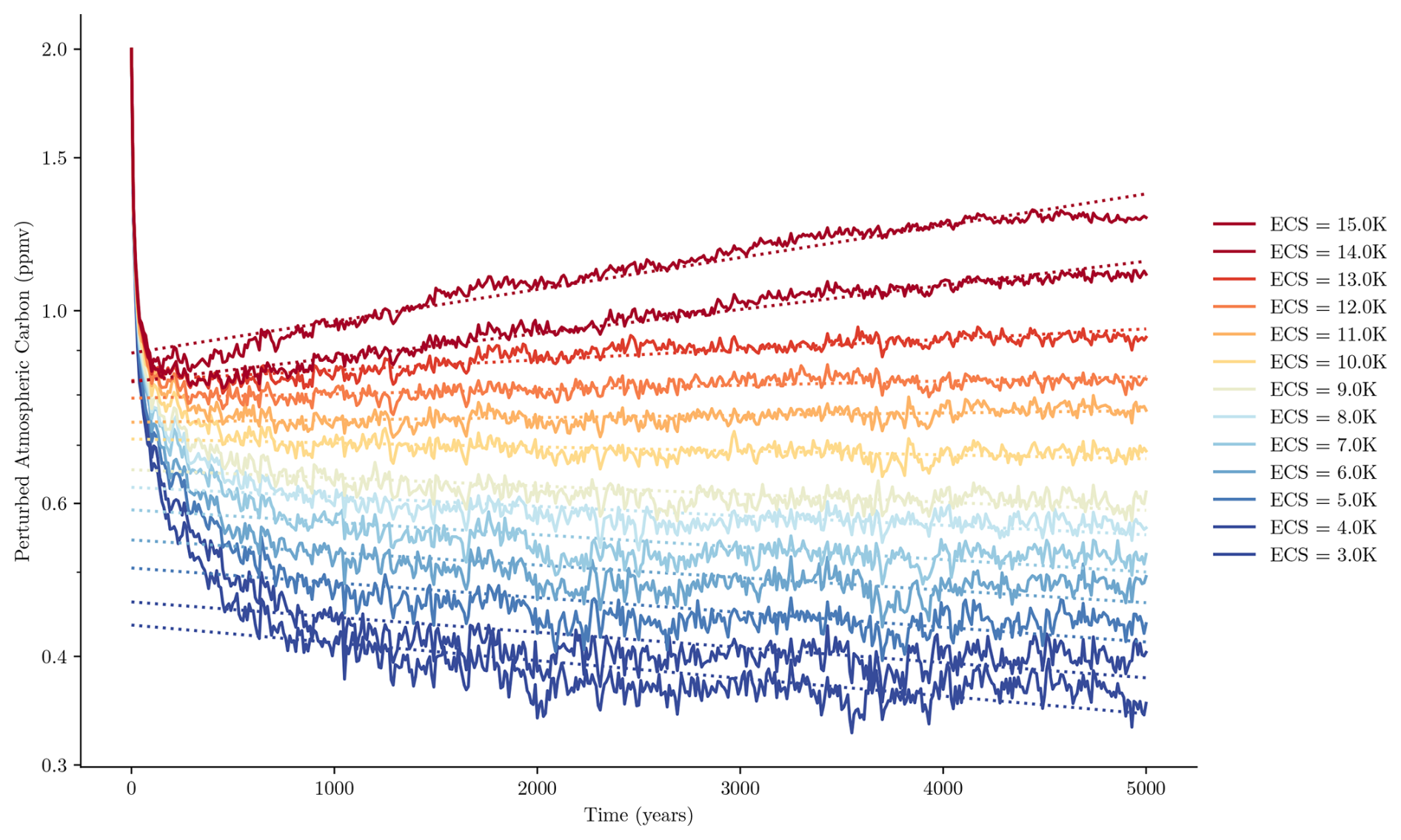
Figure 6 Atmospheric CO₂ from a JULES run for a variety of different climate sensitives. The system was initialised from an equilibrium state and given a perturbation of 2 ppmv of CO₂. After an initial transient the atmospheric CO₂ changes exponentially with time, which corresponds to a linear change on a logarithmic scale. In dotted lines we plot fits of exponential growth or decay to the latter portion of the time series. As ECS increases, the system transitions from stable exponential decay to unstable exponential growth.

Figure 7 The growth rates of CO₂ as estimated from the time series shown in Fig. 6. Fitting Eq. (12) gives the blue line. The x-intercept gives the critical ECS at which the bifurcation occurs. The estimated critical ECS is 10.9 ± 0.6 K.

3.3 Results

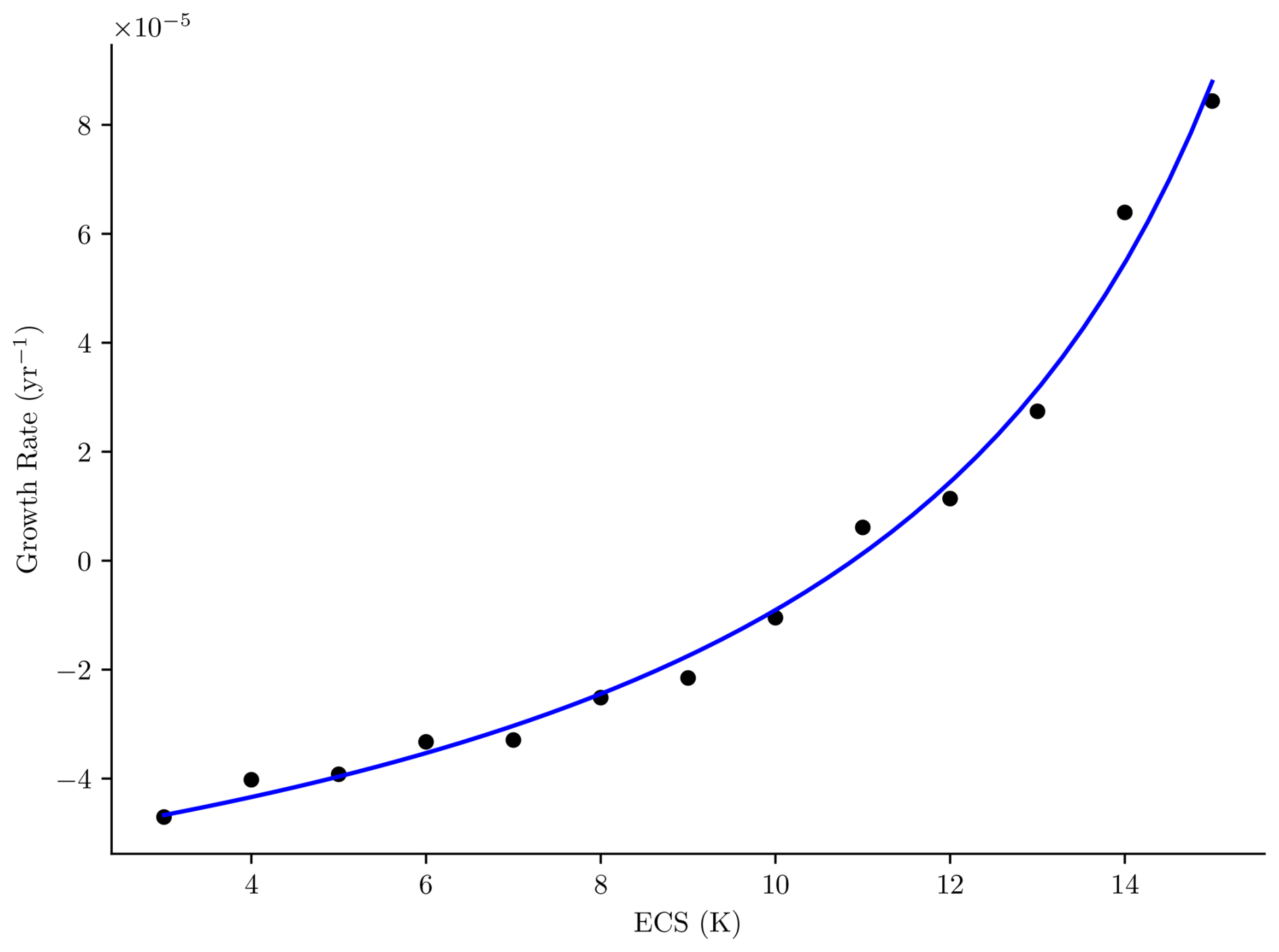
The results of this experiment are plotted in Fig. 6. The figure shows the changing CO₂ levels for different values of ECS. CO₂ levels show exponential change over a millennial timescale. The CO₂ changes are all consistent with exponential growth or decay, although it is possible we are detecting a very long period oscillation. For large enough ECS values, there is exponential growth, indicating an unstable steady state, but for smaller values of ECS the system undergoes exponential decay, indicating a stable steady state. The growth rates, given by the slopes of these lines, are plotted in Fig. 7 against ECS.

Figure 7 shows the growth rates of atmospheric CO₂ as a function of ECS. The curve given by Eq. (12) was fitted to this data to enable estimation of the critical ECS value, which occurs when the growth rate is 0. The critical ECS value was found to be 10.9 ± 0.6 K, where the uncertainty is given by a 95 % confidence interval. This compares remarkably well with the prediction of the simple model, with the central estimate matching its prediction.

This unstable growth in JULES/IMOGEN is associated with a decrease in global soil carbon (see Fig. S4 in the Supplement). Furthermore, soil carbon and heterotrophic respiration in JULES are modelled in a similar way to how we have modelled them in the simple model, suggesting that the instability in IMOGEN/JULES and the instability in the simple model share a common mechanism. Furthermore, the agreement between the simple and complex model on the critical ECS value suggest that the simple model captures the relevant processes needed to determine the stability of the climate–carbon system.

4 Discussion and conclusions

In this paper, we examined the conditions under which the positive feedback loop between heterotrophic respiration and global warming could lead to an unstable, runaway growth in atmospheric CO₂. We examined a simple conceptual model of the climate–carbon cycle system to explain this mechanism. To test the results of the simple model, we performed experiments with the coupled climate–carbon model JULES/IMOGEN.

Using the parameters in Table 1, the simple model predicts that the pre-industrial climate–carbon state can undergo a Hopf bifurcation. We were able to derive a formula for the critical parameters at which this bifurcation occurs. In particular the simple model is unstable for equilibrium climate sensitivities above 10.9 K. This critical value is outside the likely range of ECS of 2.6–3.9 K (Sherwood et al., 2020), which is consistent with the observed stability of pre-industrial climate–carbon cycle state.

The parameters in Table 1 are generally realistic, as they are based on the outputs of complex models that reproduce observed climate change. The main exception however is our choice of the alkalinity, Alk. We have an unrealistically high value, which leads to too much carbon stored in the ocean. A lower, more realistic, choice of Alk would tend to make the system less stable as it would reduce the ocean's ability to take up carbon. However, a lower choice of Alk would mean that the ocean model could not reproduce the observed change in ocean carbon over the historical period.

Some unrealistic assumptions were made about the climate–carbon system. For example, we neglected the effect of temperature change on NPP and CO₂ solubility, which tends to destabilise the system. Furthermore, we ignored spatial heterogeneity and assumed two boxes were sufficient to capture the climate response, although in fact three may be optimal (Cummins et al., 2020). These unrealistic assumptions are particularly acute after the Hopf bifurcation where the limit cycle pushes the system into extreme regions of phase space (such as at very high or very low CO₂).

We were also able to use the JULES/IMOGEN model to estimate the critical equilibrium climate sensitivity which leads to instability, which was also determined to be around 10.9 K. Unlike the simple model, this model does not neglect temperature feedbacks on NPP or ocean carbon uptake. Furthermore it is fully spatially resolved, and does not make unrealistic assumptions about the alkalinity of the ocean. However, due to computational constraints we are not able to run JULES/IMOGEN for long enough to see what state the model tends to after the instability. Furthermore, we were not able to run the model for long enough to determine whether the increase in CO₂ is a genuine instability or just the start of a decaying oscillation.

Both modelling approaches have complementary strengths and weaknesses. The qualitative agreement between the models (an instability occurring around 11 K driven by heterotrophic respiration) therefore indicates a robustness to our conclusions.

That climate–carbon instability can play a role in Earth system, specifically paleoclimate, dynamics has long been appreciated. For example Saltzman and Maasch (1988) showed how unstable interactions between physical climate and ocean carbon uptake could lead to oscillations resembling the Pleistocene glacial-interglacial cycles. More recently, Boot et al. (2022) showed how ocean circulation can induce a Hopf bifurcation in the carbon cycle, potentially explaining some CO₂ variability. On longer timescales, Hülse and Ridgwell (2025) demonstrated that different carbon cycle processes could “out-compete” the silicate weathering thermostat, leading to significant cooling. The carbon cycle may also be excitable (Rothman, 2019), meaning small perturbations lead to large responses. Extreme fluctuations can be seen in isotopic records which show a heavy-tailed distribution (Arnscheidt and Rothman, 2021). Carbon cycle instability can even be seen in high CO₂ exoplanets (Graham and Pierrehumbert, 2024). This paper (and Cox et al., 2006) is unusual in that it studies an instability in the interaction of the terrestrial biosphere with the physical climate.

Although our analysis has focused on the pre-industrial climate–carbon equilibrium, we can apply our results to a wider range of climate–carbon cycle states. We must be working on timescales long enough that there is a steady state CO₂ concentration, $C_{\mathrm{A}}^{\ast }$, to which the climate–carbon system has equilibrated but short enough that astronomical forcing and carbon cycle changes due to silicate weathering can be neglected.

For example, we may consider a future climate state with elevated CO₂ levels caused by anthropogenic emissions. Perhaps counter-intuitively, this state may be more stable than the pre-industrial climate as the critical ECS scales with atmospheric carbon.

Conversely, climate–carbon states with lower atmospheric carbon, for example at the Last Glacial Maximum (LGM), are less stable. The size of the CO₂ fertilisation effect differs across CMIP6 ESMs, although the JULES prediction is close to the ensemble mean (Varney et al., 2023). We find that if CO₂ fertilisation of photosynthesis is negligible, perhaps due to strong nitrogen limitations, then the LGM state is unstable for a critical ECS of 4.5 K, which is within the CMIP6 range. This instability may manifest, as it does in the JULES/IMOGEN run, as a continual drift in atmospheric CO₂ concentrations.

It is natural to ask if any CMIP6 models are unstable. Whilst it is possible that modelling groups may “tune away” this instability, it may persist in other models. One reason may be that this instability occurs slowly, so it may not be detectable over the typical duration ESMs are run for. More fundamentally, the most widely used CMIP experiments (such as piControl, 1pctCO2, abrupt-4xCO2, historical and the SSP scenarios) are forced with prescribed concentrations of CO₂, rather than dynamically updating CO₂ concentrations due to the carbon cycle. This cuts the feedback loop between warming and respiration. Therefore, even if ESMs were unstable, this would not be apparent in typical CMIP simulations.

However, there is a push to run CMIP7 ESMs with dynamically updated CO₂ (Sanderson et al., 2024). If the CMIP7 ensemble, like CMIP6, continues to include ESMs with a large climate sensitivities then it is possible the climate–carbon instability may arise. Although our central parameter estimates give a critical ECS of 10.9 K for the pre-industrial state, we find that if the CO₂ fertilisation effect is weak enough then the critical ECS becomes 6 K, just on the edge of the CMIP6 range. However we expect models in an LGM configuration to be unstable at even lower climate sensitivities.

In summary, we have examined the possibility of an instability within the climate–carbon system. This instability is caused by a positive feedback loop between global temperatures and heterotrophic respiration. We find that this instability can only occur for sufficiently high ECS. Our analysis suggests that the high ECS values of some ESMs combined with a weak CO₂ fertilisation effect may not be compatible with a stable glacial climate.