Intensity and dynamics of extreme cold spells of the 21st century in France from CMIP6 data

Cold extremes significantly impact society, causing excess mortality, strain on healthcare systems, and increased demand on the energy system. With global warming, these extremes are expected to decrease, as observed in various indicators. This study simulates extreme cold spells of 15 d using a stochastic weather generator (SWG) based on circulation analogues and importance sampling, adapted for CMIP6 data. Our results show that the most extreme cold spells decrease in intensity with global warming, making 20th-century-like events (e.g., 1985 in France) nearly impossible by the end of the 21st century. However, some events of similar intensity may still occur in the near future. Such events are associated with patterns of atmospheric dynamics that convey cold air from high latitudes into Europe. Those atmospheric circulation patterns show a consistent high-pressure system over Iceland and a strong low-pressure system over southwestern Europe in ERA5 and CMIP6 models. We show that nudging the SWG towards this type of pattern triggers extreme cold spells, even in a warmer world. We also show that most CMIP6 models accurately represent this atmospheric pattern. This study highlights the importance of understanding cold spell dynamics and the relevance of rare events algorithms and large ensemble models to simulate low-probability, high-impact events, offering insights into the future evolution of cold extremes.

1 Introduction

Cold extremes have significant impacts on society, with cold weather being linked to excess mortality and morbidity (Conlon et al., 2011; Masselot et al., 2023). Although mortality from heat extremes is increasing with global warming, more deaths are still attributable to cold extremes (Gasparrini et al., 2015), and healthcare systems in the mid-latitudes experience higher pressure during winter (Charlton-Perez et al., 2019).

Cold spells also have significant impacts on energy systems, affecting both energy demand and power supply, as investigated in numerous studies (Añel et al., 2017; Bessec and Fouquau, 2008; Bloomfield et al., 2016; Davies, 1959; Jacob et al., 2018; Panteli and Mancarella, 2015; Pardo et al., 2002; Sailor, 2001; Thornton et al., 2016; Van Der Wiel et al., 2019). For instance, in February 2021 Texas was hit by a severe cold snap that led to cascading failures in the energy system, resulting in a power outage and leaving millions of Texans without electricity (Busby et al., 2021). While those temperatures were extreme, they were not unprecedented. However, population growth and ongoing electrification made the system more vulnerable to such extreme events (Doss-Gollin et al., 2021).

In France, the historical cold spell of January 1985 led to peaks in electricity demand and power outages (Caud and Vautard, 2018; Le Monde, 1985; RTE, 2021). More recently, the cold spell of February 2012 caused a record consumption of electricity and put the energy network at risk (Le Monde, 2012a, b). In 2023, the electricity transmission system operator Réseau de Transport d'Électricité (RTE) gave a warning about the winter season ahead because, for several reasons, there would be tension in the electricity supply – lack of gas supply due to the economic and geopolitical context combined with the unavailability of parts for the nuclear power plants for technical reasons – potentially leading to outages in the event of high demand caused by a cold spell (RTE, 2023b). The resulting reduction in electricity consumption and the overall mild winter allowed the avoidance of power outages in France. However, RTE stated that up to 12 red Écowatt signals (power cut inevitable without a reduction of consumption) could have been raised otherwise (RTE, 2023a). Rouges et al. (2025) recently analyzed the impact of atmospheric patterns on energy shortfalls in Europe due to cold temperatures and the lack of wind. Therefore, even in a warmer world, cold events remain a main concern for the energy systems, especially in case of increased vulnerability or when facing an energy crisis (RTE, 2021).

As the lower atmosphere warms due to climate change, it is expected that cold extremes will decrease (Seneviratne et al., 2021). Warming trends have already been detected across various indicators, such as cool nights (TN10p) and the coldest night of the year (TNn), as reported in observations and reanalysis studies (Donat et al., 2016; Morak et al., 2013). Statistical analyses also show a faster decrease in all-time daily low records than compared to a stationary climate (Finkel and Katz, 2018). Attribution studies on specific events, such as the winter of 2010 in Europe, have shown that these recent extreme events would have been even more extreme without climate change (Cattiaux et al., 2010; Christiansen et al., 2018). Similar analyses performed on climate model simulations to investigate the evolution of cold events in the future also indicate a continuation of the frequency decrease in cold extremes from several key indicators (Coppola et al., 2021; Gross et al., 2020; Kim et al., 2020; Thorarinsdottir et al., 2020; Wehner et al., 2020).

From a physical point of view, winter cold spells in Western Europe are typically caused by a blocking event over Greenland, the North Atlantic, or Scandinavia that disrupts the prevailing westerly flow into Europe and allows the advection of cold air from the Arctic and Russia (Bieli et al., 2015; Buehler et al., 2011; Brunner et al., 2018; Pfahl and Wernli, 2012; Pfahl, 2014; Sillmann et al., 2011; Sousa et al., 2018). This blocking is often associated with a large cyclone over the Adriatic and Ionian seas. Although the existence of the blocking is crucial, its localization can vary. European cold winter extremes are often large-scale events affecting different regions simultaneously, which explains why the North Atlantic Oscillation (NAO) is a good indicator of cold extremes in Western Europe. A persistent negative phase of the NAO (NAO−) is often linked to long-lasting atmospheric blocking in the North Atlantic, with a cold anomaly located downstream or south of the blocking (Cattiaux et al., 2010; Greatbatch, 2000; Kautz et al., 2022; Pfahl, 2014; Seager et al., 2010; Sillmann et al., 2011; Thompson and Wallace, 2001; Wang et al., 2010).

Nevertheless, there are uncertainties surrounding the impact of Arctic amplification and the Atlantic meridional overturning circulation (AMOC) on cold extremes. For instance, these phenomena could increase the meanders of the jet stream, leading to more frequent and intense cold spells (Geen et al., 2023), although this mechanism remains debated (Blackport and Screen, 2020). The inherently low occurrence of very extreme events makes them difficult to study because of the resulting lack of samples. For instance, ≈ 3000 years of data are needed to have a 95 % probability of having at least one occurrence of a millennial event: $P_n(X\ge \mathrm{1})=\mathrm{0.95}$ for n=2994, where X is the number of occurrences of an event with a yearly probability of $p=\mathrm{1}/\mathrm{1000}$ and n the number of years during which that event could occur. So if we consider a 50-year climate period, even a large simulation ensemble of up to 50 members is not sufficient to ensure the occurrence of at least one millennial extreme event.

To address this, various methods rooted in statistical physics have been developed to simulate realistic extreme atmospheric variables. Rare events algorithms based on importance sampling (e.g., Ragone et al., 2018; Ragone and Bouchet, 2021) have been developed to specifically simulate extreme heatwaves from climate models by selecting and cloning trajectories that are most likely to lead to extremes. Gessner et al. (2021) proposed a similar approach (so-called ensemble boosting), selectively targeting climate model trajectories yielding higher temperatures and running new ensembles of perturbed reinitialized clones at the starting points of these trajectories. Sippel et al. (2024) adapted this method to extreme cold winters over a specific region (Germany). Finkel and O’Gorman (2024) demonstrated that ensemble boosting is quite optimal to simulate short-lived (up to 2 weeks) extreme events.

Another approach employs stochastic weather generators (SWGs), which are Markov processes generating large ensembles of atmospheric trajectories with realistic statistics at minimal computational expense (Ailliot et al., 2015). Yiou and Jézéquel (2020) integrated a SWG based on circulation analogues (Yiou, 2014) with importance sampling to specifically simulate extreme summer heatwaves from circulation analogues, enabling physically consistent trajectories of extreme events at very low computational cost.

Those algorithms were mainly developed and used to study summer heatwaves, but ensemble boosting and SWGs have both been adapted to extreme cold winter events by Cadiou and Yiou (2025) and Sippel et al. (2024). Nevertheless, those results were only applied to present-day events and limited to ERA5 reanalysis and the CESM2 climate model. Here, we apply the SWG to various CMIP6 model outputs to have a broader view of low-probability, high-impact extreme cold spells in the future. We then analyze the resulting simulations to evaluate potential changes in the intensity and dynamics of extreme cold spells in the future. Short events (1–2 weeks) are more relevant in terms of associated impacts on the energy sector (Añel et al., 2017; RTE, 2021, 2023b), therefore we focus in this study on persisting cold spells of 15 d.

Rare event algorithms primarily aim to simulate extreme events. Their nudging or score function typically maximizes the variable of interest, such as temperature, precipitation, or wind speed. However, we argue that using them with another nudging variable or score function – that does not directly involve the variable of interest, such as temperature – allows for identifying the drivers of the extremes of the variable of interest. For instance, Noyelle (2024, chap. 6) applied a rare event algorithm using soil moisture or geopotential height at 500 hPa at a grid point as score functions to investigate their effect on high temperatures. Similarly, in this study, we further analyze the link between North Atlantic atmospheric dynamics and extreme cold spells in France by running SWG simulations with empirical importance sampling on the dynamics instead of temperature in order to isolate the effect of dynamics on the extremeness of the event.

This paper is organized as follows: Sect. 2 presents the data used in the study. Section 3 presents the statistical model used and the various experiments conducted with it. Results are presented in Sect. 4. First, we evaluate how the intensity and dynamics of extreme cold spells evolve with climate change in CMIP6 models. Then, we investigate more precisely the role of dynamics in extreme cold spells in both the present and future. Finally, discussions and conclusions appear in Sect. 5.

2 Data

In this paper, we investigate the evolution of cold spells in France in the ERA5 reanalysis dataset (Hersbach et al., 2020) and in an ensemble of CMIP6 model simulations (Eyring et al., 2016). ERA5 was chosen for its extensive time coverage (from 1950 to the present day) and its high horizontal resolution of 0.25°. CMIP6 was chosen to allow the intercomparison of several global climate models (GCMs) for future projections.

The domain of interest for temperature is metropolitan France. We consider daily average temperature (TG). The daily temperature values of ERA5 and CMIP6 are interpolated on the Système d'Analyse Fournissant des Renseignements Adaptés à la Nivologie (SAFRAN Vidal et al., 2010) reanalysis grid, with a horizontal resolution of 8 km. Then a mask of metropolitan France is applied to have a more accurate weighting of continental surfaces. We then compute the daily spatial average of temperature over metropolitan France.

CMIP6 models all yield temperature biases (cf. Fig. 1). There are many sophisticated ways of correcting model biases (François et al., 2020), but those methods are generally not appropriate for extremes. Therefore, we simply apply a first-order bias correction by removing the difference in medians of December to February (DJF) temperature means from 1950 to 2000 (as displayed in Fig. 1) between each model and ERA5. This avoids the generation of artifacts on extremes due to bias correction methodologies.

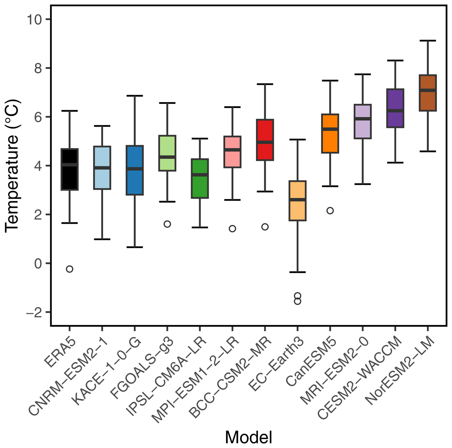
Figure 1 Empirical probability distributions of December to February mean temperatures (without mean correction) over France from 1950 to 2000 for ERA5 (black) and the 11 CMIP6 models (colors) in Table 1. In the box plots, the boxes represent the median (q50), with the lower and upper hinges denoting the first (q25) and third (q75) quartiles, respectively. The upper whiskers are defined as $min[max(T),q\mathrm{75}+\mathrm{1.5}\times (q\mathrm{75}-q\mathrm{25}\left)\right]$, while the lower whiskers are formulated symmetrically. The individual points in the plot correspond to the outlying values that exceed the upper whisker or fall below the lower whisker.

To characterize the atmospheric circulation, we use the mean daily geopotential height at 500 hPa (Z500). The preference for Z500 over sea-level pressure (SLP) is motivated by its lower dependence on disturbances originating from surface roughness, as well as its widespread utilization in the study of weather regimes, as substantiated by several studies (Corti et al., 1999; Dawson et al., 2012; Jézéquel et al., 2018; Yiou and Nogaj, 2004). Jézéquel et al. (2018) highlighted that Z500 is more suited for simulating European temperature anomalies, even though their investigation was centered on warm summer temperatures.

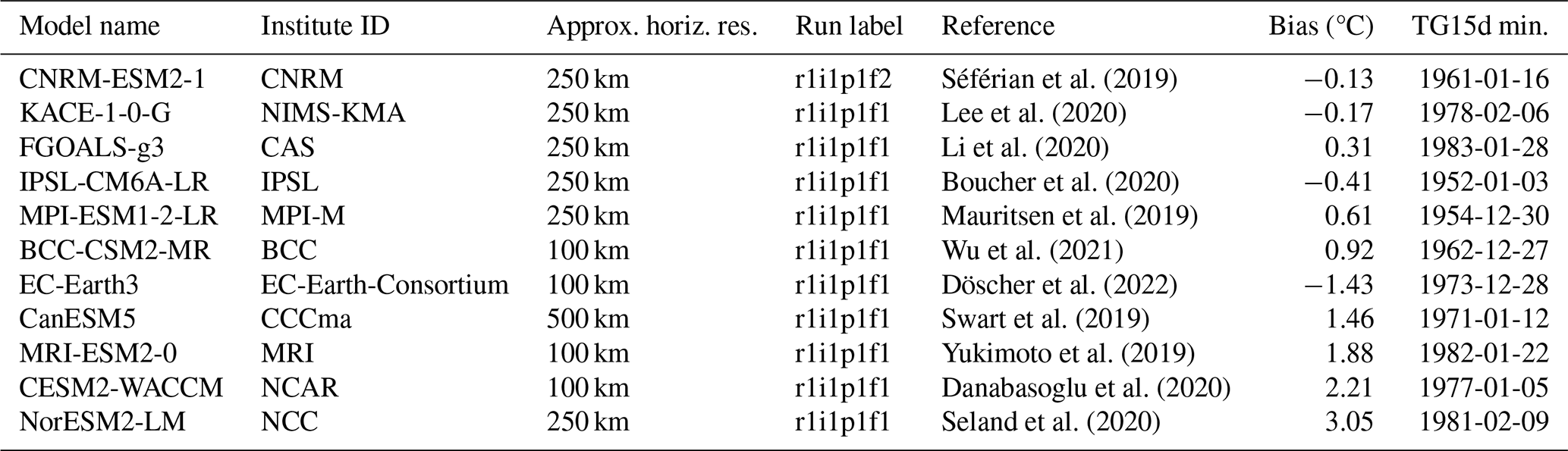
We selected 11 models out of 34 CMIP6 models. The selection criterion is the availability of daily temperature and Z500 data on the IPSL meso-center. For simplicity, we considered only one model run when ensembles were available. The resulting list of models is specified in Table 1. The horizontal resolutions range from 100 to 500 km.

Séférian et al. (2019)Lee et al. (2020)Li et al. (2020)Boucher et al. (2020)Mauritsen et al. (2019)Wu et al. (2021)Döscher et al. (2022)Swart et al. (2019)Yukimoto et al. (2019)Danabasoglu et al. (2020)Seland et al. (2020)

Table 1 List of selected CMIP6 model runs. The selection criterion is the availability of daily data for Z500 and temperature on the IPSL computing server. The bias is computed as the difference in medians of December to February temperature means over France from 1950 to 2000 between each model and ERA5. The last column indicates the date of occurrence of the coldest TG15d event in the historical simulation (1950–2014).

To provide a first-order evaluation of the accuracy of these models for winter temperatures over France, we compute the DJF temperature averages (over metropolitan France) for each winter from 1950–1951 to 1999–2000 and compare the distributions with ERA5. The bias is then calculated as the difference between the median of the model and ERA5. Results are presented in Fig. 1 and Table 1. The mean DJF bias ranges from −1.43 to +3.05 °C, with 7 out of 11 models displaying a positive bias and 4 exhibiting a negative bias with respect to ERA5. CNRM-ESM2-1, KACE-1-0-G, FGOALS-g3, and IPSL-CM6A-LR exhibit the lowest bias (in absolute value). We performed a Kolmogorov–Smirnov (K–S) test of the similarity between the winter temperature distributions of ERA5 and each “raw” CMIP6 model simulation (the null hypothesis is that the distributions are the same). This null hypothesis could not be rejected for those four models with the lowest biases (p>0.05). The computed bias was removed from daily temperature data for each model. This performs a first-order bias correction as mentioned at the beginning of this section. This bias estimation offers an initial approximation of the model accuracy for winter temperatures in France. We use it as a correction to allow a better comparison to ERA5 data, but it does not necessarily indicate that a model with low bias is proficient for accurately simulating extreme cold spells in France. After this mean bias removal, the null hypothesis that ERA5 and CMIP6 simulations yield the same DJF probability distributions cannot be rejected for all considered model simulations with a K–S test.

To investigate the projected climate until 2100, we selected four shared socioeconomic pathways (SSPs; Riahi et al. (2017)) to cover the broad range of future plausible socioeconomic and climatic scenarios: SSP1-2.6, SSP2-4.5, SSP3-7.0, SSP5-8.5. For each model, we computed the global mean surface temperature (GMST), and its yearly increase from the 1950–2000 average.

To compute atmospheric circulation analogues, we used Z500 anomalies over the North Atlantic spatial domain (20° W–30° E; 30° N–70° N) as outlined by Cadiou and Yiou (2025). Anomalies of Z500 were computed on a daily basis, subtracting the seasonal cycle as a 31 d moving average computed on the 1981–2010 reference period. Z500 increases as a result of the warming of the atmosphere due to the expansion of the lower atmosphere. Therefore a linear trend was removed for each Z500 grid-point before computing the analogues for each model and scenario.

3 Methods

3.1 Analogues–SWG

We first establish a database of circulation analogues, following the methodology outlined by Yiou and Jézéquel (2020). For any specific day t, we calculate the (spatial) Euclidean distance between the Z500 fields of day t and all other days t^′, ensuring these days do not fall within the same year or season (straddling two consecutive years) and maintain a calendar distance from t that is less than 30 d (i.e., $|t-t^{\prime }|\le \mathrm{30}$ d). The K best analogue days for t are identified as the K days with the minimum distance from t. In line with recommendations from prior research (Platzer et al., 2021), we select K=20 best analogues.

To study the evolution of cold-spell atmospheric dynamics from 1950 to 2100, we compute circulation analogues in three non-overlapping periods of 50 years:

1. 1950–1999: past period over which we can compare CMIP6 and ERA5 data.

2. 2000–2049: present-near future period in CMIP6. The rationale for considering this period is that SSP scenarios barely differ before 2050.

3. 2050–2099: future period in CMIP6.

For CMIP6 models, the historical period (1950–2015) is concatenated to the run of each SSP (2015–2100). This results in a 150-year file for each model and SSP, which is then divided into three non-overlapping climate periods of 50 years. Therefore, the first analogue period (1950–1999) is common to the four SSPs, while separate sets of analogues are computed over 2000–2049 and 2050–2099 for each SSP. The period 1950–1999 is used for comparison with ERA5.

The SWG developed by Yiou (2014) uses circulation analogues to generate alternative trajectories of temperature or precipitation values by reshuffling daily atmospheric fields. This algorithm was modified by Yiou and Jézéquel (2020) to simulate extreme heat waves using importance sampling and by Cadiou and Yiou (2025) to simulate extreme cold winter events from the ERA5 reanalysis. As we want to simulate extreme cold spells, we hereafter use the version of the SWG developed by Cadiou and Yiou (2025).

The SWG starts at a given initial condition and proceeds to the next time step using analogues of circulation and information on their “next day.” The simulation is a constrained reshuffling of days from the input dataset. At each time step, the selection of the analogue day is subject to constraints and weights that are controlled by model parameters explained below, so that the sampling is not necessarily uniform among the K best analogues and the circulation of the next day.

To follow the seasonal cycle, K+1 weights ${\mathit{\omega }}_{\mathrm{cal}}^{\left(k\right)}$ are used, depending on a parameter α_cal that favors analogue days and the next day t+1 closest to the calendar date of time step t:

$$\begin{array}{}\text{(1)}& {\mathit{\omega }}_{\mathrm{cal}}^{\left(k\right)}=A_{\mathrm{cal}}{e}^{-{\mathit{\alpha }}_{\mathrm{cal}}{d}_k}.\end{array}$$

To simulate the most extreme events, importance sampling weights ${\mathit{\omega }}_T^{\left(k\right)}$ are introduced, with a control parameter α_T≥0. The higher α_T is, the more the SWG favors analogue days with extreme temperatures. The K analogues of t and the Z500 pattern of day t+1 are sorted in ascending order of temperature with ranks $R_k\in \mathit{\{}\mathrm{1},\mathrm{\dots },K+\mathrm{1}\mathit{\}}$:

$$\begin{array}{}\text{(2)}& {\mathit{\omega }}_T^{\left(k\right)}=A_T{e}^{-{\mathit{\alpha }}_T{R}_k}.\end{array}$$

Note that the K+1 values of ${\mathit{\omega }}_T^{\left(k\right)}$ are the same from one time step to the next because they do not depend on the temperature value but on the rank of the circulation analogues temperature.

The SWG with importance sampling is achieved by combining the calendar and importance sampling weights. The probability of sampling the kth analogue day of day t (or the Z500 pattern in day t+1) is given by

$$\begin{array}{}\text{(3)}& {\mathit{\omega }}_k=A{e}^{-{\mathit{\alpha }}_{\mathrm{cal}}{d}_k}{e}^{-{\mathit{\alpha }}_T{R}_k}\end{array}$$

where A is a normalizing constant ensuring that the sum of all probabilities ω_k equals 1.

3.2 Protocol of SWG simulations

To evaluate the impact of climate change on extreme 15 d cold spells, we make SWG simulations of extreme cold events from the three different climate periods and the four SSPs, i.e., using the analogue sets computed for each. For each model, we identify the coldest TG15d in the historical period (1950–1999). Those dates are indicated in Table 1. Then we initialize the SWG at the starting date of that event and run 1000 simulations per analogue period (1950–1999, 2000–2049, and 2050–2099) and scenario (SSP1-2.6, SSP2-4.5, SSP3-7.0, SSP5-8.5). Thus, $\mathrm{1000}\times \mathrm{3}\times \mathrm{4}$ simulations are made for each of the 11 climate models. Simulations made for 1950–1999 should be very similar across SSPs as the analogue set used is the same. This SWG simulation protocol is an innovation compared to the simulations of Cadiou and Yiou (2025), as non-overlapping analogue periods are considered, as well as a multi-model ensemble, rather than just a reanalysis. For comparison over the historical period, we perform 1000 simulations starting on 3 January 1985 (beginning of the coldest TG15d in ERA5) using ERA5 analogues from 1950 to 1999.

This SWG approach of running alternative trajectories of pre-existing extreme events is similar to the “ensemble boosting” method of Gessner et al. (2021). The ensemble boosting approach starts by identifying the most extreme events in a long control simulation of a climate model. Then the model is initiated a few days before the apex of the extreme, and ensembles are run from small perturbations of the initial condition (Gessner et al., 2021). The ensemble boosting procedure keeps the most extreme simulations. It has been argued that such an approach is optimal to simulate short-lived extremes (Finkel and O’Gorman, 2024). The SWG approach was previously applied to the study of potential future heatwaves by Yiou et al. (2023), who ran ensembles of simulations starting before an identified heatwave in each model for different SSPs. The main difference with the study of Yiou et al. (2023) is that major cold spells occurred in the 20th century, while the most intense heatwaves are bound to occur toward the end of the 21st century.

The same approach was also used by Cadiou and Yiou (2025) using the single observed event of winter 1963 as a reference. That study focused on whole winter events over the available period of ERA5 data (1950–2021). Here, we use the SWG over a wide range of climate model data and SSPs to gain a broader view of the evolution of 15 d cold spells in the future, both in terms of intensity and dynamics.

In this paper, we chose to give equal weights to all GCM simulations by considering only one member of each ensemble, i.e., the first in lexical order of the run names, as done in many studies (e.g., Christiansen, 2020; François et al., 2021; Huang et al., 2024). As some research groups have provided GCM ensembles with many members, we checked our results when starting the SWG simulations from alternative runs (see Appendix A). This verification emphasizes the importance of large ensemble of GCM simulations (Bevacqua et al., 2023). We defer the systematic study of large ensembles of GCM simulations to another paper.

3.3 Atmospheric circulation index for cold spells

Cold spells in France are generally associated to an easterly or northeasterly flow of cold air, which can be either dry or humid (e.g., Yiou and Nogaj, 2004). These flows are typically caused by an anticyclone around Iceland or Scandinavia, which leads to a weakening of the westerlies and allows the outbreaks of cold air. These weather patterns can persist for up to a week or 10 days, with temperatures dropping significantly, especially during nighttime clearings on snow-covered grounds in humid episodes. These mechanisms are strengthened by an anticyclone over southern Europe.

Z500 mean anomalies maps during the coldest 15 d cold spells in ERA5 show a dipole between Iceland and southwestern Europe. Therefore, to investigate the dynamics of cold spells in France, we compute a Western Europe cold circulation index (WCC), which characterizes this atmospheric pattern, by subtracting the mean of Z500 between (1° W–9° E; 40° N–47° N) and (24° W–13° W; 62° N–66° N). Those areas were chosen as the maximum and minimum of the dipole structure identified from the Z500 composite map of the 20 coldest cold spells in France from ERA5. As shown in Fig. 4, the WCC is correlated to daily temperature over France during winter months (Pearson correlation coefficient r=0.65 and $p<{\mathrm{10}}^{-\mathrm{15}}$). As this WCC index is tailored for a specific type of event (15 d cold spells) over a specific region (metropolitan France), it performs better than a classic daily North Atlantic Oscillation (NAO) index, defined as the normalized SLP difference between the Azores and Iceland (r=0.36 and $p<{\mathrm{10}}^{-\mathrm{15}}$).

To facilitate the comparison between models, the WCC index was normalized to $(-\mathrm{1},\mathrm{1})$. The normalization was done by subtracting the mean value and dividing by the range (max minus min) of the data:

$$\begin{array}{}\text{(4)}& x_{\mathrm{normalized}}={\displaystyle \frac{x-x_{\mathrm{mean}}}{x_{max}-x_{min}}},\end{array}$$

where x is the Z500 difference. Therefore, an index of −1 corresponds to the most extreme dipole observed in ERA5, characterized by a strong high-pressure system over Iceland and a strong low-pressure system over southwestern Europe. An index of 1 corresponds to the opposite configuration, with a low-pressure anomaly over Iceland and a high-pressure anomaly over southwestern Europe. This normalization allows for the identification of atmospheric configurations that tend towards the identified dipole, with more negative values indicating a stronger and more intense pattern.

3.4 SWG with importance sampling on circulation

After analyzing the atmospheric dynamics of extreme cold spells and its evolution between 1950 and 2100, we want to evaluate the role of the atmospheric circulation in triggering cold spells over France. To this end, we run simulations of the SWG, applying the importance sampling to WCC instead of temperature. We call these new simulations WCC-SWG, as opposed to T-SWG where the importance sampling is on temperature. In this way, no direct incentive is given to temperature in the SWG simulations. The SWG is only parameterized to favor trajectories with a low WCC, i.e., with a Z500 configuration tending towards a dipole featuring a high over Iceland and a low over Western Europe. This allows us to identify the effect of this atmospheric pattern on temperatures in France. This aims to show to what extent the identified atmospheric circulation is sufficient to trigger extreme cold spells over France. This analysis is also an innovation from the paper of Cadiou and Yiou (2025).

Results are compared with SWG simulations putting the importance sampling over temperature (as in previous simulations), a simple NAO index (NAOi; computed between the two grid points closest to the stations located in Iceland and the Azores as in Rogers (1984)), and no importance sampling (α_T=0). They will be referred as T-SWG, NAO-SWG, and control-SWG respectively.

For each model, we also fit an autoregressive model of the first order (AR(1)) on WCC anomalies over winter months, which acts as a control:

$$\begin{array}{}\text{(5)}& X_t=c+\mathit{\phi }{X}_{t-\mathrm{1}}+{\mathit{ϵ}}_t,\end{array}$$

where c is a constant and ϵ_t is a centered Gaussian white noise with standard deviation σ (${\mathit{ϵ}}_i\sim N(\mathrm{0},{\mathit{\sigma }}^{\mathrm{2}})$). The parameters ϕ and σ are estimated in a standard way by assuming that X_t and the WCC variations have the same variance and auto-covariance at lag 1 (Storch and Zwiers, 2002). The numerical values of estimated parameters are computed for each model and scenario. For instance, for KACE-1-0-G and SSP1-2.6, $\widehat{\mathit{\phi }}=\mathrm{0.859}$, $\widehat{\mathit{\sigma }}=\mathrm{0.151}$, and $c=-\mathrm{0.316}$. The AR(1) has the same autocovariance as the winter WCC of each model but is not a measure of atmospheric circulation, so it should not have any effect on temperatures. We then simulate SWG trajectories that minimize the AR(1) values (AR-SWG simulations).

This procedure defines an alternative way to causal networks (Kretschmer et al., 2021) to explore a causal relation between an atmospheric feature and extreme cold spells in France. The principle of this simple approach is to nudge toward extremes several “candidates” for causality (here, the WCC and NAO atmospheric indices) and determine the effect on the extremes of a climate variable (here, temperature). This reflects the spirit of the “do” action outlined by Hannart et al. (2016): the experimenter intervenes to set a possible driver X at a chosen value and evaluates the causal effect of X on the variable of interest Y by examining the resulting “interventional” distribution of Y.

4 Results

4.1 Intensity of winter cold spells in CMIP6

4.1.1 Extreme TG15d in model output

First, we examine the five coldest TG15d events (after bias adjustment) in ERA5 and each of the 11 CMIP6 models across the historical period and the four SSPs, all merged together (Fig. 2a). We find that only one model (EC-Earth3) is able to simulate extreme TG15d cold spells as cold as those observed in ERA5. The other models are between 0 and 3 °C above such low temperatures. EC-Earth3 simulates an event with a temperature of −8.1 °C on 28 December 1973, while the coldest event recorded in ERA5 is −7.5 °C on 1 October 1985. Despite the upward temporal trend in temperatures in all models, some models still simulate extreme cold TG15d events in high emissions scenarios or late in the century. For example, MPI-ESM1-2-LR simulates an event with a temperature of −5.8 °C on 20 October 2048 under SSP5-8.5, while IPSL-CM6A-LR simulates an event with a temperature of −4.9 °C on the 18 January 2060 under SSP1-2.6. Although those events occur in a warmer climate, they are still comparable to the coldest events recorded in ERA5 at the end of the 20th century, such as −5.0 °C on 15 January 1987 or −4.8 °C on 29 January 1963. However, they are more than 2 °C warmer than the coldest event recorded in ERA5 (−7.5 °C). No model can produce colder events after the historical period (beyond 2015).

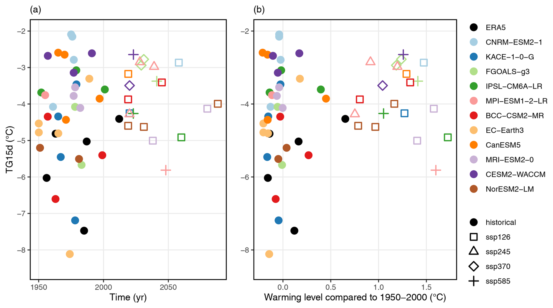
Figure 2 Five coldest 15 d 2 m temperature means (TG15d) in ERA5 from 1950 to 2023 (black circles) and in 11 CMIP6 models (colors) from 1950 to 2000 across the historical period and the four emissions scenarios (shapes) (a) by date and (b) by level of warming compared to 1950–2000. Temperatures are adjusted by the median December to February temperature bias.

We plotted the five coldest cold spells by level of warming compared to 1950–1999 (Fig. 2b). We show that half of the coldest cold spells occur for levels of warming under 0.2 °C compared to 1950–2000. A few high-intensity events are still found for higher levels of warming (TG15d of −4.9 °C in IPSL-CM6A-LR for a warming of 1.7 °C, and a cold spell reaching −5.8 °C for a warming of 1.6 °C compared to 1950–2000 in MPI-ESM1-2-LR). However, for all models, none of the five most intense cold spells happen for a level of warming higher than 1.8 °C compared to 1950–2000.

4.1.2 Extreme TG15d in CMIP6 with a SWG

To explore the evolution in terms of intensity and dynamics of extreme cold spells in the future, we run SWG simulations from CMIP6 data from 1950 to 2100, as described in Sect. 3.2. For each model, we run simulations starting at the beginning of the coldest event found in the model run over the historical period of 1950–1999 (see Table 1). We produce 1000 simulations for each of the 50-year periods and each of the four SSPs. The discrepancies between models observed in the TG15d cold spells simulated by the SWG are similar to those found in the cold events detected in the “raw” model runs (Fig. 3). In the historical period (1950–1999), the median temperature of the SWG simulations varies significantly, with the coldest model (EC-Earth3) reaching a temperature of −5.3 °C and the warmest model (IPSL-CM6A-LR) reaching a temperature of 0.0 °C. In comparison, the median temperature of the ERA5 simulations for the same period is −3.9 °C. These results indicate that there are substantial differences between the models, even in the historical period, and that most of the models are warmer than the ERA5 simulations even after correcting by the historical DJF mean. The SWG simulations from KACE-1-0-G, BCC-CSM2-MR, MRI-ESM2-0, and NorESM2-LM manage to display a distribution that is comparable to ERA5 SWG simulations according to a K–S test. The results in the following sections will focus on the first model (KACE-1-0-G), as it also yields a low mean bias (Fig. 1).

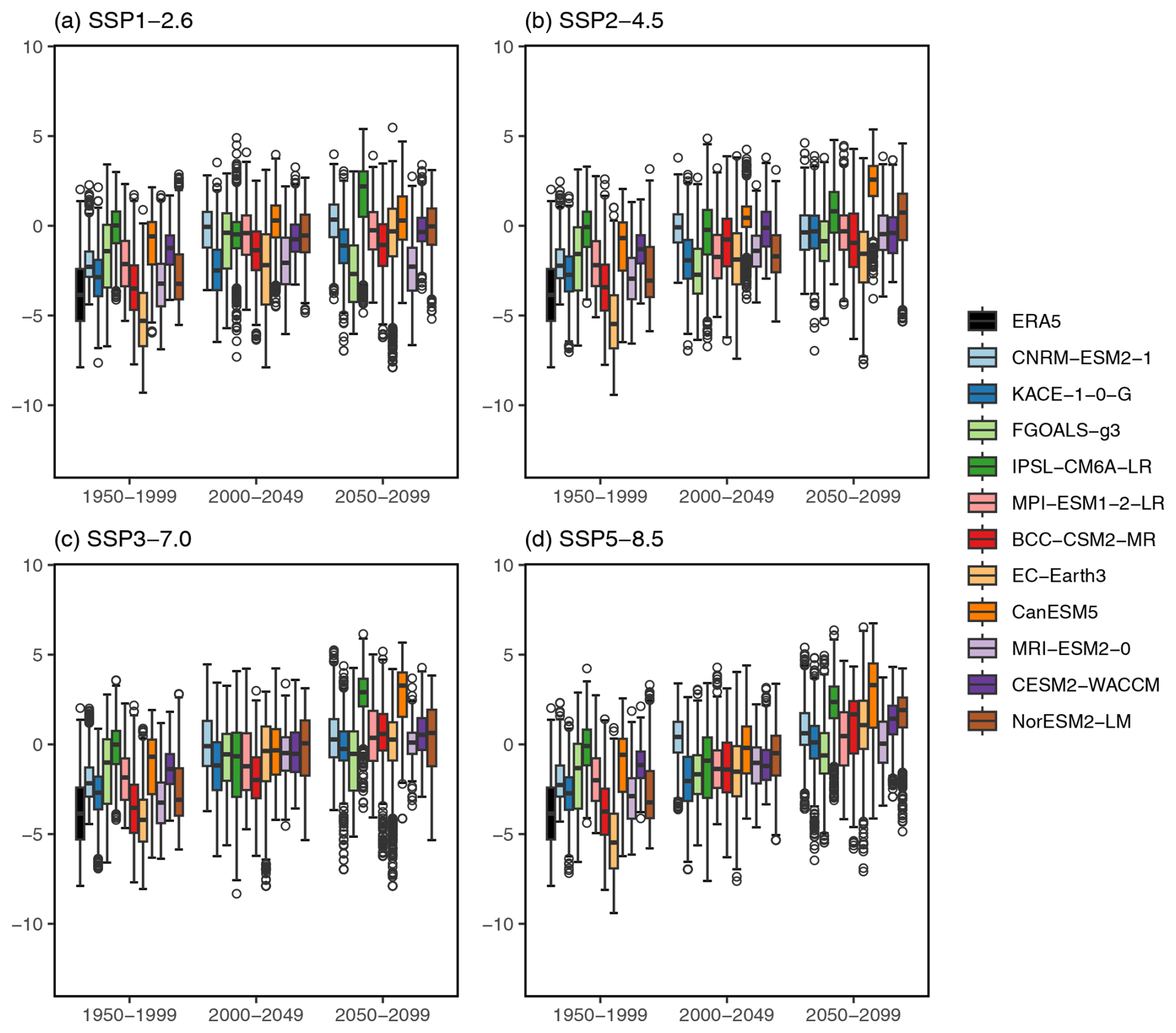
Figure 3 TG15d (in °C) of stochastic weather generator simulations of 15 d cold spells for ERA5 (black, only 1950–1999 analogue period) and CMIP6 models (colors), for four socioeconomic pathways (SSPs) ((a) SSP1-2.6, (b) SSP2-4.5, (c) SSP 3-7.0, (d) SSP5-8.5) and three analogue periods (1950–1999, 2000–2049, 2050–2099). Each boxplot displays TG15d for 1000 simulations. Temperatures are adjusted by the median December to February temperature bias. In the boxplots, the boxes represent the median (q50), with the lower and upper hinges denoting the first (q25) and third (q75) quartiles, respectively. The upper whiskers are defined as $min[max(T),q\mathrm{50}+\mathrm{1.5}\times (q\mathrm{75}-q\mathrm{25}\left)\right]$; the lower whiskers are $max[min(T),q\mathrm{50}-\mathrm{1.5}\times (q\mathrm{75}-q\mathrm{25}\left)\right]$. The individual points in the boxplot correspond to the outlier values that exceed the upper whisker or fall below the lower whisker.

Out of the 11 models examined, only two (EC-Earth3 and BCC-CSM2-MR) allowed SWG simulations of TG15d events colder than the coldest ERA5 event in the historical period for the runs we considered. This implies that the remaining models may be underestimating the potential intensity of future cold waves. However, we note that the models that produced the coldest events in the historical period also exhibited the fastest warming rates. Consequently, the disparity in the extreme cold events simulated by the different models at the end of the 21st century is not as wide. For instance, under SSP5.8-5 the standard deviation of the simulations for the period 1950–1999 is 2.1 °C, compared to 1.9 °C for the period 2050–2099.

If more runs from the same model are considered (e.g., with the IPSL-CM6A-LR model; see Appendix), this cold event (in ERA5) is potentially more common. This is probably due to internal multidecadal variability.

In the present-day period (2000–2049), the impact of climate change on cold spells is limited across all scenarios, as more than half (between 6 or 7 out of 11 depending on the scenario) of the models still simulate extreme cold events that are colder than the ERA5 median for the period 1950–1999. However, as the level of warming increases toward the end of the 21st century in high-emissions scenarios, the likelihood of very extreme cold events, comparable to the cold events of 1963 or 1985 in the 21st century, becomes negligible in all scenarios. The coldest TG15d event simulated by the SWG in the period 2050–2099 under the SSP5-8.5 scenario, obtained from EC-Earth3 analogues, reaches a temperature of $\approx -\mathrm{7}\mathit{°}$C over France, but stands as an outlier.

4.2 Dynamics of winter cold spells

4.2.1 Atmospheric dynamics of very intense cold spells in CMIP6

To investigate whether models reproduce the same atmospheric dynamics leading to cold spells as in ERA5, we computed the WCC index for each model and scenario. In all 11 CMIP6 models, the daily winter temperature over France is significantly correlated with the WCC (p-value $<{\mathrm{10}}^{-\mathrm{15}}$), although the correlation is not as strong as in ERA5. The correlation ranges from 0.45 in CanESM5 (which is the model with the coarsest resolution) to 0.56 in CESM-WACCM and MRI-ESM2-0. If a 1 d shift is considered between the WCC and temperature, the correlation is higher, ranging from 0.49 for CanESM5 to 0.61 for CESM-WACCM. This suggests that the WCC measures how the atmospheric circulation is related to the advection of cold air into France, hence triggering cold spells. Correlation does not imply causality and essentially measures the covariations of “small” fluctuations of temperature and WCC. Here we are interested in the way a very low value of WCC impacts temperature, and hence identify a causal connection that was suggested by the correlation.

We first determine the distribution of the WCC probability distribution for the events previously simulated with the SWG. This helps us assess whether a low value of WCC is a necessary condition for cold spells (i.e., the behavior of WCC when TG15d is cold). The results are shown in Fig. 4. For most models, the identified cold spell episodes lead to negative values of WCC, indicating that they are associated with the identified dipole of Z500. However, some models (CanESM5, FGOALS-g3, NorESM2-LM) have mostly positive WCC values, suggesting that they have difficulty reproducing the same patterns that lead to very extreme cold spells as observed in ERA5. For instance, CanESM5 is also the model that had the weakest correlation between the WCC and winter daily temperature over France, which can be explained by its coarse resolution (≈500 km). Those models still produce a similar dipole pattern in the Z500 field during the events they simulate. However, the high-pressure center in the dipole in some models is shifted to the south of Iceland (IPSL-CM6A-LR) or towards Scandinavia (NorESM2-LM or EC-Earth3 for instance), and the low-pressure center is shifted to the west (FGOALS-g3) compared to the dipole pattern observed in ERA5 (See Supplement Figs. S1 to S10).

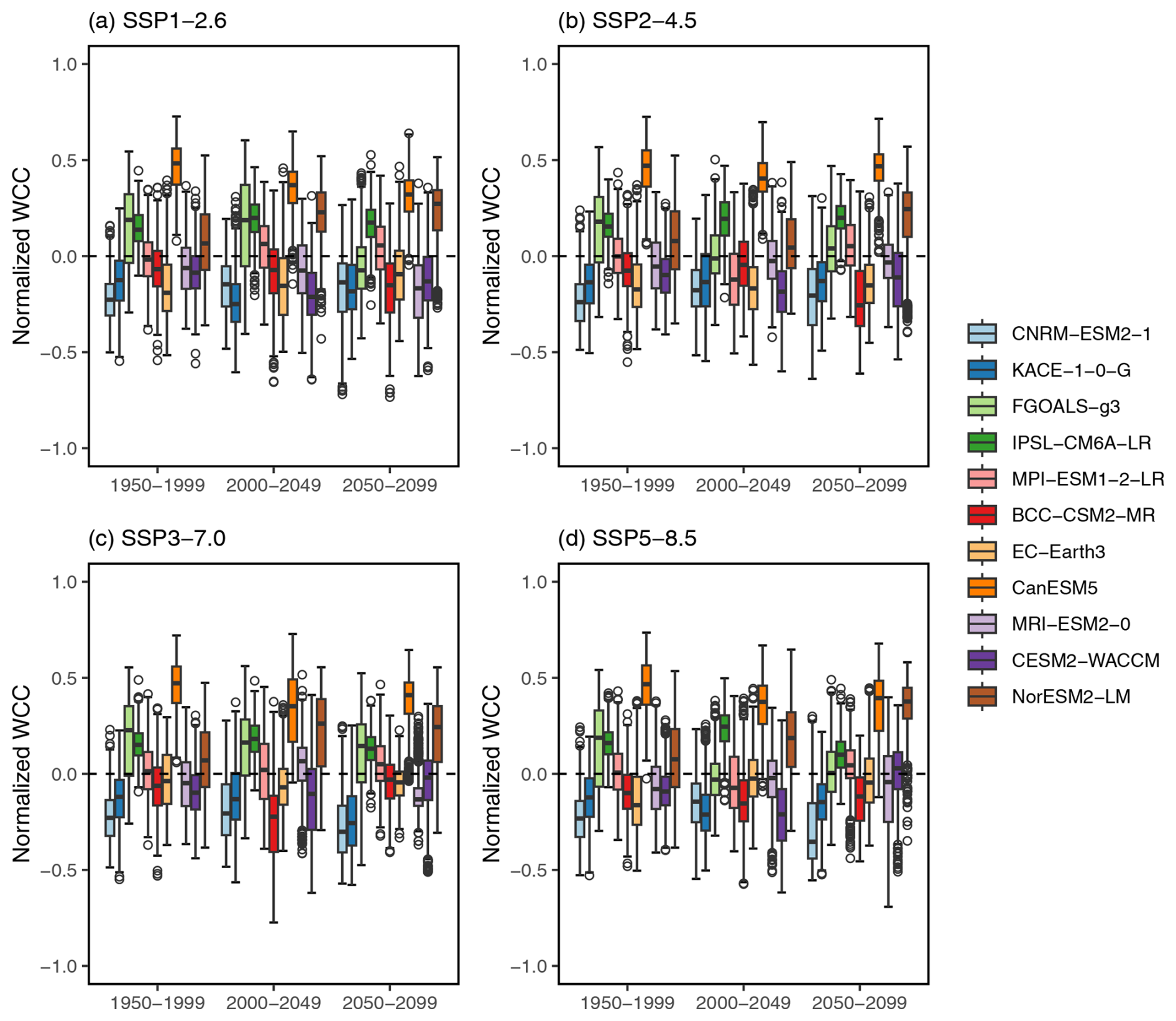
Figure 4 Normalized Western Europe cold circulation index (WCC) composites (normalized values) of the stochastic weather generator output simulations for each CMIP6 model and period, for SSP1-2.6 (a), SSP2-4.5 (b), SSP3-7.0 (c), and SSP5-8.5 (d). A negative value shows the presence of a dipole of Z500 between Iceland and southwestern Europe. Boxplots are defined as in Fig. 3.

The maps (Fig. 5) and the WCC values (Fig. 4) show that there is no significant change in the dynamics of cold spells with high levels of warming. In Fig. 4, more than half of models have a negative median WCC in SWG simulations. Models that have the most positive values are CanESM5 and FGOALS-g3, which are models that struggled in producing extreme cold events comparable to ERA5 with the SWG (see Fig. 3). We also note that CanESM5 is the model with the coarsest resolution. KACE-1-0-G has the majority of its SWG simulations with negative WCC whatever the period or SSP. The values of the WCC are fairly consistent across periods and scenarios within each single model. This suggests that the mechanisms driving these events are not significantly affected by climate change in the CMIP6 models that we consider. Even if global warming affects the intensity of this type of events, it does not cause major changes in their dynamics in those models.

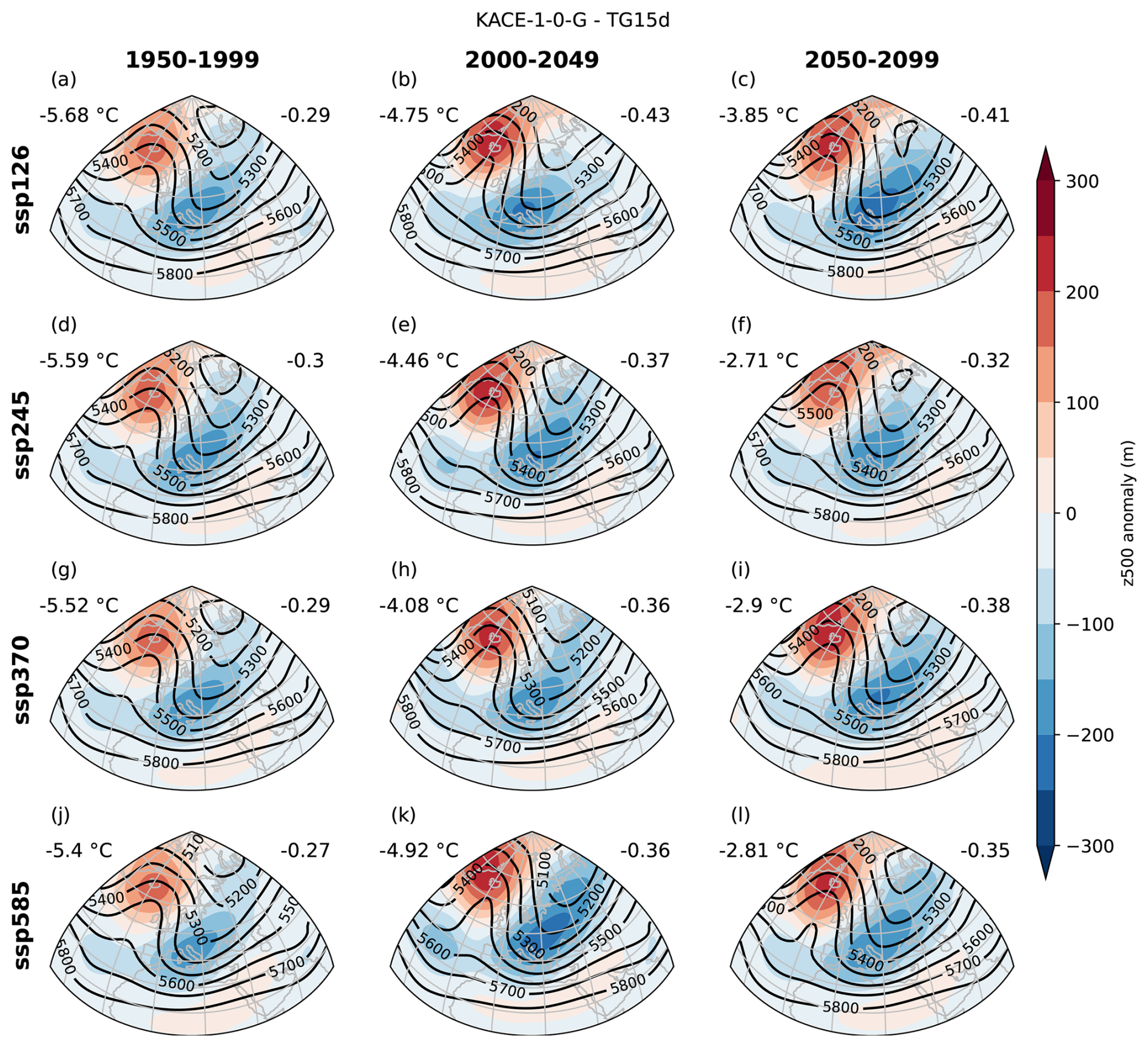
Figure 5 Absolute values (contours, in m) and anomalies (shaded areas, in m) with respect to 1950–1999 of 500 hPa geopotential height (Z500) for the 10 % coldest stochastic weather generator simulations (i.e., 100 trajectories) for each period (columns) and shared socioeconomic pathways (SSP) (rows) in KACE-1-0-G. Each map displays the adjusted composite temperature on the top left and the composite normalized Normalized Western Europe cold circulation index (WCC) on the top right.

To ensure that the composite maps are representative of the dynamics of individual simulations, we computed the standardized standard deviation of Z500 from the 10 % coldest SWG simulations, for each grid point. The standard deviation was calculated from the 100 coldest simulations (out of 1000 SWG simulations) and normalized by the climatological standard deviation of Z500 for each climate model. This adjustment for each grid point was necessary because Z500 exhibits greater variability in the high latitudes than in the low latitudes. The results for KACE-1-0-G are presented in Fig. 6. The simulations demonstrate a high degree of similarity of Z500 maps over Europe and the North-East Atlantic between SWG simulations. This outlines the relevant atmospheric features to trigger winter cold spells in France. Those areas are very consistent across periods, scenarios, and models (see Supplement Figs. S11 to S20). Some models do have a larger standard deviation between simulations (FGOALS-g3 or CanESM5) but most of the domain still has a standardized standard deviation under 1, which means that simulations are more alike than random days.

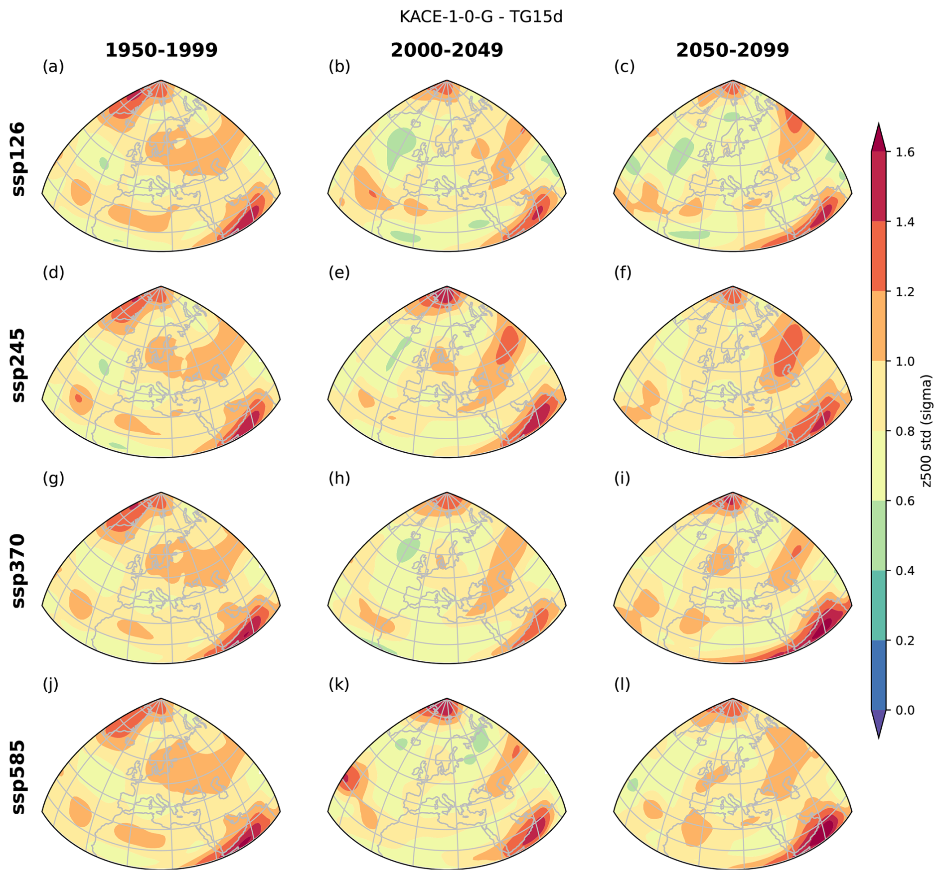
Figure 6 Standardized standard deviation (shaded areas, σ) and anomalies with respect to 1950–1999 standard deviation of 500 hPa geopotential height (Z500) for the 10 % coldest stochastic weather generator simulations (i.e., 100 trajectories) for each period (columns) and shared socioeconomic pathways (SSP) (rows) in KACE-1-0-G.

4.2.2 Role of atmospheric conditions to generate cold spells

In this section, we evaluate how an atmospheric circulation pattern leads to a cold event. In the previous section we investigated the mean atmospheric patterns that prevail during cold spells. This corresponds to assessing the necessary atmospheric patterns for a cold spell. Conversely, we now evaluate how those atmospheric patterns lead to extreme cold spells, which corresponds to a sufficient condition. Such a sufficient condition can be anticipated by the 1 d lag between the WCC index and temperature. Here, we verify that this relation holds for the most extreme events.

We test this hypothesis by running SWG simulations with importance sampling weights on the WCC index (WCC-SWG) rather than temperature (T-SWG). Hence, the SWG simulations exacerbate the effects of this bipolar atmospheric pattern. No nudging is added on temperature, so that the sole driver of the temperature simulated by the SWG is the atmospheric circulation. For comparison purposes, SWG simulations are also performed with importance sampling weights on temperature (as in Sect. 4.1.2), an NAO index (NAO-SWG), an AR(1) process (defined in Sect. 3.4, AR-SWG), and with no importance sampling (control-SWG). Results are shown for the KACE-1-0-G model and SSP5-8.5 in Fig. 7. The results for other models and SSPs are shown in Supplement Figs. S21–S30. Very consistently across models, scenarios, and periods, WCC-SWG simulations yield temperatures that are as cold as T-SWG simulations, even for models that did not accurately reproduce the WCC distribution. In comparison, AR-SWG and control-SWG simulations produce events with milder temperatures, corresponding to an average TG15d event in winter for each period and scenario. NAO-SWG simulations are overall colder than AR-SWG and control-SWG but do not reach the cold temperatures of T-SWG simulations. This demonstrates that atmospheric circulation is the main driver of cold extremes in France and that an index tailored for this region and event type performs well in capturing the circulation associated with these extreme events.

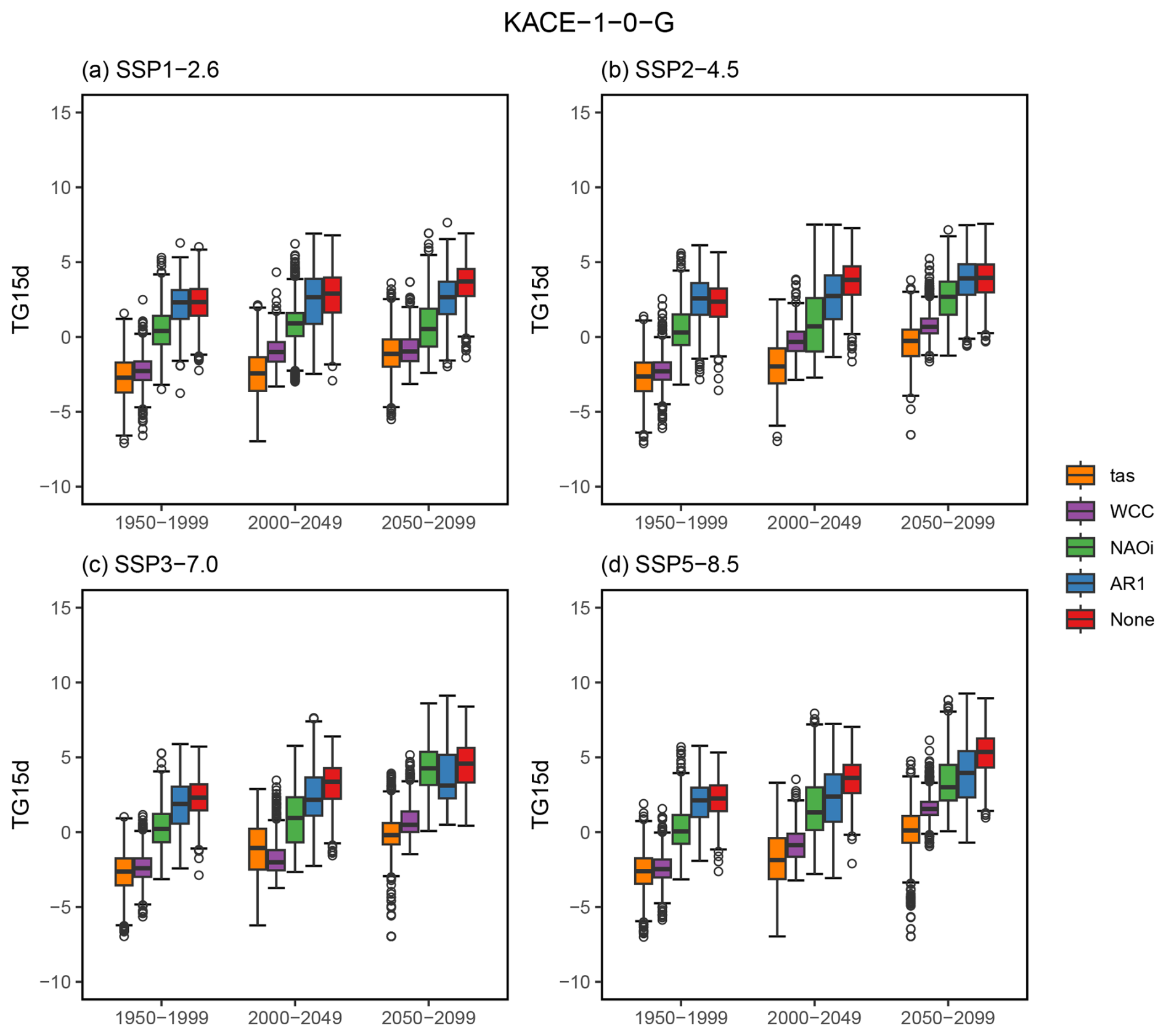
Figure 7 Temperature (TG15d) distribution of 1000 stochastic weather generator (SWG) simulations for four shared socioeconomic pathways (SSPs) (a–d) and three climate periods (left to right in each panel) depending on the variable used for importance sampling (colors). The SWG simulations are obtained with the KACE-1-0-G model. Temperatures are adjusted by the median December to February temperature bias. Box plots are defined as in Fig. 3.

Therefore, a dipole featuring a high over Iceland and a low over Western Europe is a sufficient condition to trigger extreme 15 d cold spells over Western Europe in the selected CMIP6 models, even in a climate with a higher level of warming.

The upward trends across the three epochs are similar between the forcing variables (Fig. 7). Cadiou and Yiou (2025, Fig. 1) have shown that the trends of the coldest 15 d events in ERA5 are similar to the whole DJF trends for France. Therefore, the increase of SWG temperatures reflects the mean increase of winter temperatures (in France).

To assess the evolution of the atmospheric pattern, we first determine the 5th percentile of the winter daily WCC for the historical period of each model. For each year between 1950 and 2100, we then compute the number of winter days with WCC falling under that threshold. We compute a yearly linear regression of this number of days. The trend in the number of days that fall below this percentile is computed for each model and scenario. The significance of the trend is assessed by a Mann–Kendall test (Storch and Zwiers, 2002). As depicted in Fig. 8, about half of the models do not exhibit a significant trend. We emphasize, a model could yield a decrease in the frequency of low WCC days with warming, while still displaying a low WCC when an extreme cold spell occurs. Between models that do yield a trend, there is a substantial disparity in the direction of potential trends. However, the trends are largely consistent across scenarios for a single model, indicating that the dynamic evolution is coherent within individual models.

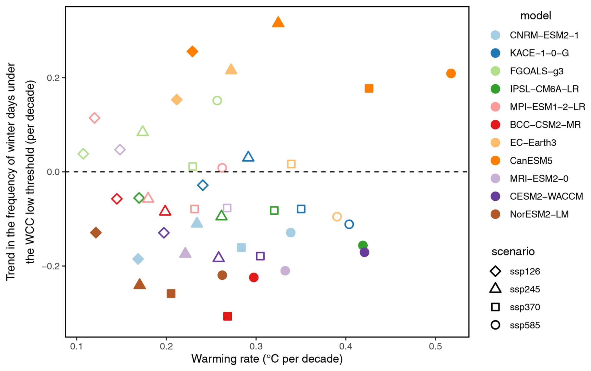
Figure 8 Yearly trend in the frequency of low Western Europe cold circulation index (WCC) days by global warming rate between 1950 and 2100 for each of the 11 CMIP6 (colors) and scenarios (shapes). Filled points outline the cases for which the WCC trend is significant according to a Mann–Kendall test.

We find that 14 runs (from 6 different models, as we consider 4 SSPs per model) yield a significant negative trend, while only 6 runs (from 2 models) exhibit a positive trend. Therefore, among the models selected for this study, the majority of models exhibit a negative trend of low WCC, although those trends are not necessarily significant. However, the GCM whose extreme cold spells in the historical period are the closest to ERA5 (KACE-1-0-G) does not yield any significant trend in any of the scenarios. Overall, the disparity between climate models makes it challenging to ascertain whether the identified pattern will increase or decrease in the future, irrespective of the scenario.

5 Conclusions

In Cadiou and Yiou (2025), we showed that cold records of the 20th century could be broken in the 21st by applying the SWG with importance sampling to ERA5 data. In this study, we extended the findings of Cadiou and Yiou (2025) to 11 CMIP6 models to examine the evolution of extreme cold spells in the future in France and to evaluate the ability of the models to reproduce the mechanisms leading to cold spells as observed in the ERA5 reanalysis.

Our study shows that cold spells of 15 d can still happen in France with moderate levels of global warming in the present and near future (i.e., at the 2050 horizon). This is coherent with previous works of Sippel et al. (2024) and Cadiou and Yiou (2025) which showed that extreme winter events such as those in 1962/63 could still happen in the present decades in Europe using ensemble boosting and ERA5-based SWG simulations. Therefore, adaptation to a warming climate should not dismiss the possibility of low-likelihood high-impact cold spells (Cohen et al., 2020, 2023; Kim et al., 2014; Screen et al., 2018), in particular for the transportation, health, and energy sectors. However, our results indicate that, as expected, the intensity of very extreme cold spells decreases with global warming for all CMIP6 models. Cold extremes that occurred during the end of the 20th century, such as the winter of 1962–1963 or in February 1956, become almost impossible at the end of the 21st century for high levels of warming. However, ongoing electrification in Europe and the growing population may lead to increased vulnerability if extreme cold events were to occur, even if their occurrence is decreasing. With a high rate of electrification, France has an electric consumption that increases rapidly with low temperatures compared to other European countries (RTE, 2023a). This could make France more vulnerable to very extreme cold spells, even under a reduced hazard.

We also analyzed the changes in the intensity and dynamics of extreme cold events under different emission pathway scenarios. Consistently with previous results on heatwaves (Galfi and Lucarini, 2020; Noyelle et al., 2024), we find that the most extreme cold spells in ERA5 tend to have a similar atmospheric circulation with a high-pressure system over Iceland and a strong low-pressure system over southwestern Europe. When analyzing the atmospheric circulation associated with the most extreme events in several CMIP6 models, we found that most models reproduce the same patterns of Z500 for cold spells, and that those patterns remain consistent across climate periods and scenarios. Some models display more variability in atmospheric dynamics among simulations (FGOALS-g3, CanESM5) or a similar pattern but shifted towards Scandinavia or the south of Iceland (NorESM2-LM, CanESM5). But overall, all models tend to display a dipole of Z500 for extreme cold spells, which justifies the design of a circulation index for cold spells (WCC).

This study complements the results of Ribes et al. (2025) who analyzed the probabilities of cold 30 d spells similar to that in 2012 in France in the CMIP6 ensemble. Although their approach is different (based on extreme value modeling of data), they conclude that the probability of the occurrence of an extreme cold spell like that in 2012 vanishes towards the end of the 21st century. This is qualitatively similar to our result (albeit a different event duration, and a different reference event).

We have demonstrated that the WCC circulation index is more adapted than the NAO index to predict low-temperature episodes over France. Conversely, the effect of this atmospheric pattern is singled out by nudging the SWG towards it without direct constraint on temperature. We show that the dipole of Z500 identified from the coldest events in ERA5 remains a sufficient condition to trigger extreme cold spells, even in a warmer world or in models that reproduced the mechanisms less accurately. This is coherent with the analysis of Röthlisberger and Papritz (2023, Fig. 3), who determined that the coldest temperatures in France are linked to advection and diabatic processes.

The SWG employed for the simulation of extreme cold spells yields some of the technical caveats previously highlighted by Cadiou and Yiou (2025) and Yiou and Jézéquel (2020). The SWG is constrained by input data (GCM or reanalysis) as it does not create new atmospheric states: the SWG can produce events of 15 d that are more extreme than those observed by reshuffling daily observations, but remains bounded by the daily data. Additionally, the SWG does not allow us to disentangle anthropogenic warming from potential other forcings and the natural variability of the climate system. The effect of climate variability could be averaged out by using ensembles of CMIP6 simulations, but not all ensemble simulations were available to us.

In this paper, we chose to give equal weight to all GCMs by taking only their first CMIP6 runs, which have been described as reference runs (e.g., Boucher et al., 2020). It turns out that other runs from a given GCM could yield initial conditions leading to colder SWG simulations (see Appendix A). If one is satisfied with working with single GCM data, we emphasize the necessity of considering large GCM ensembles (covering the same period of time) (Bevacqua et al., 2023) in order to sample the coldest initial conditions within the same forcing conditions.

Our study evaluates how the mechanisms of cold spells are represented in the selected CMIP6 GCMs, especially in a warmer climate. Our analysis of the WCC index indicates that most models do exhibit atmospheric patterns for cold spells that are comparable to those in ERA5 in the historical period. This WCC index is constructed for France and could be adapted for other parts of Europe to simulate cold extremes and the associated atmospheric circulation.

Appendix A: SWG simulations from the IPSL ensemble

In this appendix, we analyze how the SWG simulations of TG15d depend on the GCM run initial conditions. For practical reasons, we restrict this analysis to the IPSL model, which proposes 33 runs. In the paper, we have used the first in lexicographical order (r1i1f1p1), which has been chosen as the “reference” for the IPSL model, and used in many studies (Boucher et al., 2020).

It turns out that this reference r1i1f1p1 run yields TG15d events that are not as cold as the 32 other runs. In particular, the r11i1f1p1 run contains a TG15d event that is much colder than what is observed in ERA5 (Fig. A1).

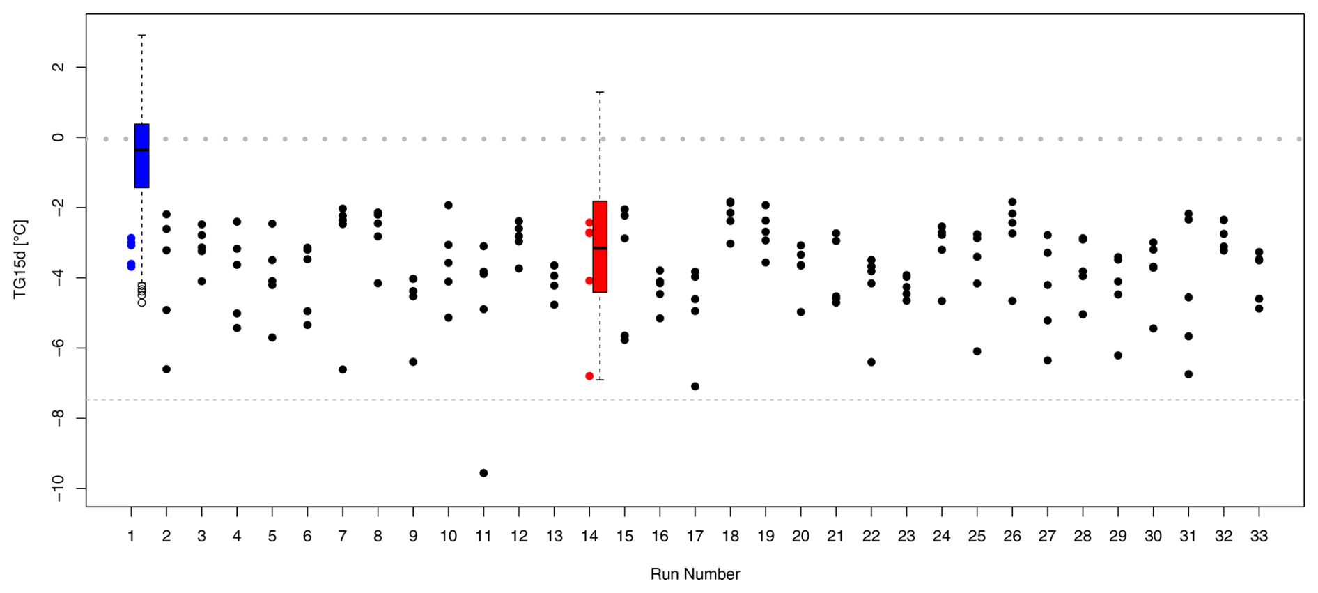
Figure A1 Temperature (after first-order bias correction) of 5 coldest 15 d cold spells (TG15d) in each of the 33 IPSL run members (r1i1f1p1 to r33i1f1p1). The blue dots on the left outline the coldest TG15d in the first run (r1i1p1f1) used in the study. The red dots are for the r14i1p1f1 run. The colored boxplots represent the empirical probability distributions of the stochastic weather generator simulations starting from the coldest blue (r1i1f1p1) or red dots (r14i1f1p1). The dashed line represents the “observed” value in 1987 in ERA5. The horizontal dotted line is the average of the yearly coldest TG15d value between 1950 and 1999 in the IPSL model runs (around 0 °C). The average value of TG15d is around 4 °C (i.e., outside of the figure).

For verification purposes, we performed SWG simulations from the coldest TG15d event in r14i1f1p1 (red dots in Fig. A1), which is not the coldest among all GCM simulations, but with TG15d events that are colder than that obtained with r1i1f1p1. The rationale of this choice is to select an extreme cold event that is not too different from the other simulations (from visual inspection). This allows us to assess to what extent the SWG simulations can reach the coldest IPSL GCM events. The core of the SWG simulations lie within the range of the five coldest TG15d events, but barely colder (lower whiskers of the boxplots of Fig. A1). For r14i1f1p1, this is explained by the temporal structure of the coldest TG15d (around −7 °C), which is part of a cold spell that persists for more than 15 d. The SWG allows random switching to “less cold” events (and the weights of the analogue sampling are on the rank of analogue temperatures, not the temperatures themselves), which are indeed ≈2 °C warmer.

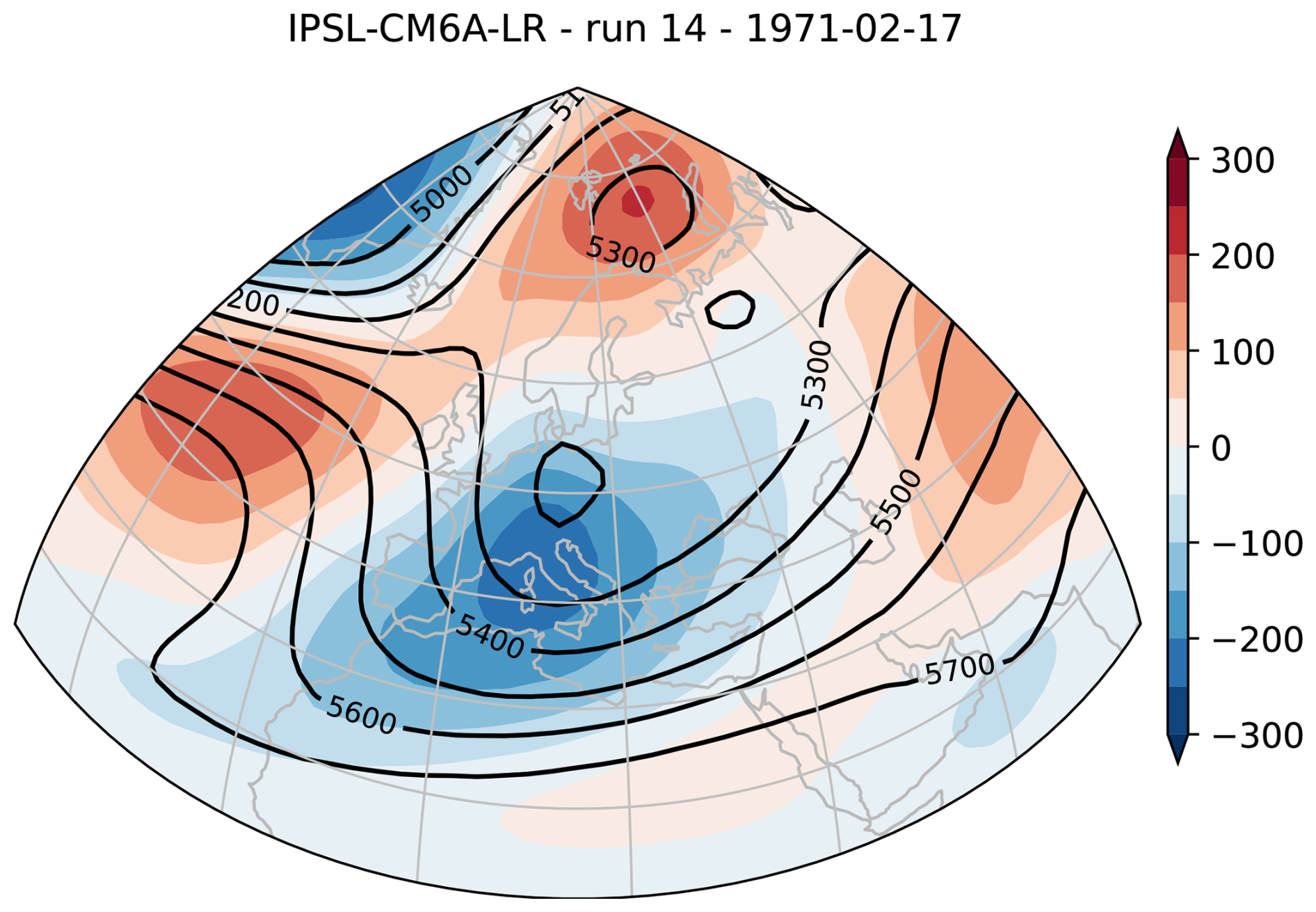
Figure A2 Absolute values (contours, in m) and anomalies (shaded areas, in m) with respect to 1950–1999 of 500 hPa geopotential height (Z500) for the 10 % coldest SWG simulations (i.e., 100 trajectories) for starting on the coldest TG15d of the IPSL-CM6-LR r14i1f1p1 run.

The importance sampling procedure is not as efficient to generate the coldest events for durations of 15 d, as for events of 90 d Cadiou and Yiou (2025), especially if the “training” data does not contain long-lasting cold events, which is the case for r1i1f1p1. But the SWG simulations are potentially colder than the average of the coldest yearly TG15d (around 0 °C in the IPSL model), and much colder than the average winter TG15d value (around 4.5 °C).

We verify that the Z500 patterns from r14i1f1p1 are similar (Fig. A2), and yield a high Z500 contrast between southern France and Ireland.

We conclude that the SWG simulations lead to conservative estimates of the coldest TG15d from climate model simulations. The quantiles of the SWG probability distributions of temperature obviously highly depend on the GCM run that is chosen.