Uncertainty quantification for overshoots of tipping thresholds

Many subsystems of the Earth system, which are currently closely following a stable state, are at risk of undergoing abrupt transitions to a drastically different, and often less desired, state due to anthropogenic climate change. These so-called tipping events often present severe consequences for ecosystems and human livelihood that are difficult to reverse. Forcing a nonlinear system beyond a critical threshold that signifies the onset of self-amplifying feedbacks constitutes a possible mechanism for tipping. However, previous work has shown that it could be possible to briefly overshoot a critical threshold without tipping. For some cases, the peak overshoot distance and the time a system can spend beyond a threshold are governed by an inverse-square law relationship (Ritchie et al., 2019). However, in the real world or in complex models, critical thresholds and other system features, such as inherent timescales and the system's linear restoring force after perturbations, are highly uncertain. In this work, we explore how such uncertainties propagate to uncertainties in the probability of tipping in response to a temporary overshoot from the perspective of uncertainty quantification. We show the importance of constraining uncertainty in the location of the tipping threshold and the linear restoring force to the system’s stable state to better constrain the uncertainty in the tipping behaviour for overshoot trajectories. We first prototypically analyse effects of an uncertain critical threshold location separately from effects due to an uncertain linear restoring force. We then perform an analysis of joint effects of uncertain system characteristics within a conceptual model for the Atlantic Meridional Overturning Circulation (AMOC). The simple box model for the AMOC shows that these uncertainties have the potential to reverse conclusions for mitigation pathways. A pathway previously associated with a low risk of tipping may become highly dangerous if the tipping threshold were to be closer than previously assumed. In this conceptual model, we illustrate how constraining the highly uncertain diffusive timescale (representative of wind-driven fluxes) within this box model reduces the tipping uncertainty of the AMOC in response to overshoot scenarios.

1 Introduction

Recently, climate tipping points have gained increasing attention from scientists, policymakers, and the public (Lenton et al., 2023), building on the previous scientific literature on the topic; see e.g. Lenton et al. (2008), van Nes et al. (2016). Tipping events are abrupt transitions that may occur if some external forcing crosses a critical threshold (Scheffer et al., 2012). Systems that are closely tracking a stable state may find their current state ceasing to exist beyond the threshold and therefore cause the system to transition (potentially irreversibly) to a drastically different state (Lenton et al., 2008). In the latter study, the authors identified tipping elements of the climate system. A recent assessment can be found in Armstrong McKay et al. (2022), where the authors elaborate on the most important tipping elements and corresponding tipping points. These tipping points pose severe threats to ecosystems and human habitat (Lenton et al., 2023). One example for a part of the Earth system suggested to exhibit tipping behaviour is the Atlantic Meridional Overturning Circulation (AMOC) (Weijer et al., 2019). A tipping of the AMOC would be likely to cause a significant cooling over northern Europe, substantially change patterns in tropical rainfall, and lead to regional sea level rise (Jackson et al., 2015). Gaining a better understanding of the tipping behaviour of the AMOC is crucial for deriving efficient climate change mitigation strategies.

Awareness of the need for action is prevalent, since the impacts are likely to be far-reaching if a system tips; see e.g. Ritchie et al. (2020). To increase the efficiency of mitigation measures, a better understanding of these tipping events and under which circumstances tipping can be prevented is crucial. For example, tipping is not instantaneous upon crossing a tipping threshold (Ritchie et al., 2024); thus a sufficient fast reversal in the forcing can return the system to its original state without tipping (Ritchie et al., 2019). To understand these overshoots of tipping thresholds, it is important to understand which mechanisms can cause a system to tip. We distinguish between noise-induced, rate-induced, and bifurcation-induced tipping (Ashwin et al., 2012). So-called noise-induced tipping can occur when fluctuations from fast processes become particularly pronounced and might cause the system to tip without a change in external forcing; see e.g. Ashwin et al. (2012), Ma et al. (2019). Alternatively, changing the external forcing too quickly can lead to a different tipping mechanism known as rate-induced tipping; see e.g. Ritchie et al. (2023) The mechanism of crossing critical thresholds that leads to tipping by (slowly) changing an external forcing is referred to as bifurcation-induced tipping. In Kuehn (2013), the author provides a mathematical framework for critical transitions in terms of bifurcation theory; see also Kuznetsov (2004) and Wiggins (2003) for further mathematical details. More recently, the universal nature of the emergence of critical transitions in physical systems was analysed in Kuehn and Bick (2021).

All three mechanisms can contribute to the uncertainty in mitigation windows, that is, how far and for how long a system may overshoot tipping thresholds and still return to the system's original equilibrium state (Ritchie et al., 2019). Since we would like to understand overshoots of tipping thresholds of global warming, which can be characterized as bifurcation thresholds, our primary focus is on better constraining the mitigation window for bifurcation-induced tipping. For some subsystems of the Earth, critical thresholds have been suggested to be at low levels of global warming (Armstrong McKay et al., 2022), such that overshoots of the threshold are becoming increasingly likely. It is important to note that, for some elements, climate model simulations have suggested that tipping might not occur, despite an overshoot, if the reversal of the forcing is sufficiently fast (Jackson and Wood, 2018a; Jackson et al., 2023). Since, for some systems, we are already very close to a level of global warming that might trigger tipping (see Fig. 2 of Armstrong McKay et al., 2022), it is crucial to quantify which exceedance level of a possible threshold might allow us to return to the original state if forcing is reversed sufficiently quickly. This overshoot mechanism has already been subject to thorough investigations (Ritchie et al., 2021; O'Keeffe and Wieczorek, 2020; Wunderling et al., 2023; Bochow et al., 2023).

However, much less is known about the impact of uncertainties on overshooting tipping thresholds. In particular, the IPCC 2021 report (Masson-Delmotte et al., 2021) emphasizes that high-impact, low-likelihood climate outcomes, to which some tipping events belong, should be part of climate risk assessments. To assess risks of tipping, a thorough handling of uncertainties is needed. One type of uncertainty related to a possible tipping of the AMOC is uncertainty in datasets, such as those for sea-surface temperature and salinity. In the context of early warning signals for tipping, an uncertainty propagation procedure to quantify the effects of dataset uncertainties on indicators of critical slowing down was recently proposed in Ben-Yami et al. (2023). Here, we focus on uncertainties in a conceptual model for the AMOC regarding choices of model parameter values (Lux et al., 2022). These uncertainties might significantly affect the mitigation window. Better constraining the mitigation window is a crucial task to gain a better understanding of overshoots in real-world climate systems. For the AMOC, the uncertainty in the critical global warming threshold is particularly pronounced (Armstrong McKay et al., 2022). There is a need for further research on overshoots of tipping thresholds (of the AMOC) under uncertainty in model parameters to quantify the mitigation window more narrowly.

Therefore, in this work, we focus on the quantification of uncertainty in overshooting tipping thresholds resulting from uncertainty in system characteristics for a given forcing profile. In particular, we illustrate our methodology for AMOC overshoot scenarios with the aim of gaining a conceptual understanding of the mechanisms involved and, in particular, how uncertainty affects the mitigation window. This is not only important for the AMOC, but for many other systems as well (Ritchie et al., 2021; Meyer et al., 2022; Bochow et al., 2023).

The remainder of the paper is structured as follows. Section 2 details the problem setup, including introducing the mitigation window for overshoots without tipping. In Sect. 3, we present how uncertainty in system parameters affects the mitigation window in the prototypical fold bifurcation setting inherent to many conceptual climate models. Thereby, we distinguish between uncertainty in (i) the location of the tipping threshold p_b and (ii) the linear restoring force proportionality constant κ. Section 4 provides results on the uncertainty in the mitigation window for a conceptual AMOC model, the Stommel–Cessi box model (Cessi, 1994), which exhibits two of these fold bifurcations. The uncertain diffusive timescale in this model entails uncertainty in both p_b and κ, thus exhibiting effects showcased in the previous section. In Sect. 5, we expand on how the results on the probability of tipping for the presented scenarios might inform decisions about alternative mitigation pathways.

2 Problem setup

Here, we consider various profiles for the change in an external forcing that have different characteristics with respect to the overshoot of the critical threshold/bifurcation value. Most importantly, we analyse these overshoots in the presence of uncertainties in model parameters of a conceptual AMOC model. These uncertainties introduce uncertainties in the time and peak overshoot distance that would still facilitate a return to the original state. More precisely, we use the Stommel–Cessi model (Cessi, 1994) to conceptually illustrate the far-reaching effect of uncertainty in wind-driven gyres and eddies, represented by the diffusive timescale parameter, on mitigation windows without tipping. This model exhibits a double-fold bifurcation; thus there exists a range of external forcing levels where the AMOC is characterized by multistability.

The aim is to develop a probabilistic extension of the work of Ritchie et al. (2019). Therein, the authors derived an inverse-square law between peak overshoot distance and exceedance time over the threshold represented by the fold bifurcation. The size of the mitigation window depends on system characteristics, such as its timescale. Here, we focus on the one-dimensional case and refer the reader to Ritchie et al. (2019) for the multi-dimensional case. Consider an ordinary differential equation that takes the form

$${\displaystyle }\dot{x}=f(x,p)$$

and exhibits a fold bifurcation at the point (x_b,p_b). We define

$${\displaystyle }{a}_{\mathrm{0}}:={\displaystyle \frac{\partial f}{\partial p}}(x_b,p_b)\text{and}\mathit{\kappa }:={\displaystyle \frac{\mathrm{1}}{\mathrm{2}{a}_{\mathrm{0}}}}{\displaystyle \frac{{\partial }^{\mathrm{2}}f}{\partial x^{\mathrm{2}}}}(x_b,p_b),$$

where a₀ is related to the inverse of the system's timescale and κ is proportional to the linear restoring force, which is a measure of the recovery rate back to the equilibrium after a perturbation of the system. The mitigation window can then be described with

$$\begin{array}{}\text{(1)}& (p_{\mathrm{peak}}-p_b)t_{\mathrm{over}}^{\mathrm{2}}<{\displaystyle \frac{\mathrm{4}}{a_{\mathrm{0}}^{\mathrm{2}}\mathit{\kappa }}}.\end{array}$$

The condition provided in Eq. (1) specifies the mitigation window in terms of the exceedance time over the threshold t_over and the peak external forcing p_peak over the critical threshold p_b.

Hence, to be within the mitigation window, the product of the squared time spent over the threshold and the peak overshoot distance needs to be smaller than a quantity that depends on system-specific parameters, which can be highly uncertain in real-world applications.

3 Prototypical fold bifurcation model

We begin by considering a simple conceptual model for tipping via the prototypical fold bifurcation given by

$$\begin{array}{}\text{(2)}& \mathit{\tau }\dot{x}=p_b-p\left(rt\right)-\mathit{\kappa }(x-x_b{)}^{\mathrm{2}}.\end{array}$$

Utilizing such a simple model allows us to isolate how uncertainty in either the location of the tipping threshold (fold bifurcation), p_b, or the linear restoring force of the starting state (proportional to κ) affects the uncertainty in the tipping behaviour. The height of the fold bifurcation is chosen to be at $x_b=x_{\mathrm{0}}-\sqrt{p_b/\mathit{\kappa }}$ such that the system is initialized at the same starting position, x₀=2.5, regardless of the threshold location or linear restoring force. For simplicity, the timescale parameter, τ, is set to unity and is inversely proportional to a₀ ($\mathit{\tau }=-\mathrm{1}/a_{\mathrm{0}}=\mathrm{1}$). The forcing profile used for all results based on the prototypical fold bifurcation is a symmetric overshoot given by

$$\begin{array}{}\text{(3)}& p\left(rt\right)={\mathrm{\Delta }}_p{\text{sech}}^{\mathrm{2}}\left(r\right(t-t_{\mathrm{peak}}\left)\right),\end{array}$$

which starts and finishes at zero and has an amplitude Δ_p; the rate of change is controlled by r.

3.1 Uncertain location of tipping threshold

Firstly, we will use the prototypical fold model Eq. (2) and only consider different realizations of the parameter for the tipping threshold location, p_b, which we consider uncertain here. Note that the linear restoring force (and the distance to the basin boundary) will be different at the same forcing level for two different threshold locations. Importantly, however, the linear restoring force and the distance to the basin boundary are the same when the systems are the same distance to their respective thresholds.

We now illustrate and elaborate on this idea further (see Fig. 1). Let us consider a single forcing profile in the form of Eq. (3), which starts at some initial level of forcing and smoothly increases to a peak level before returning back to the initial level at a mirrored rate as shown in Fig. 1a. Note again that the location of the tipping threshold will determine how far (if any) and how long the system will be beyond the tipping threshold for this single forcing profile. If the threshold is low (dotted red line), then the overshoot will be large and long, whereas a higher threshold (dotted orange line) means that the overshoot will be smaller and of shorter duration.

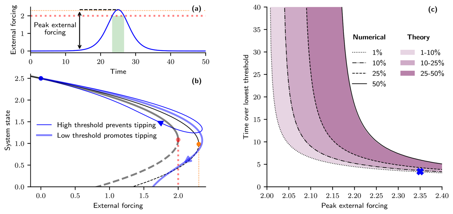
Figure 1 Probabilistic overshoots given uncertainty in the location of the tipping threshold. (a) Time profile of an exemplar external forcing given by Eq. (3) (parameters: Δ_p=2.35, r=0.24, t_peak=25). Red and orange dotted lines indicate low (p_b=2) and high (p_b=2.3) tipping threshold locations respectively. (b) System responses (blue) subjected to the external forcing profile given in panel (a) for the model given by Eq. (2) with fixed κ=1 but with either a low threshold, p_b=2 (thick and translucent curves), or a high threshold, p_b=2.3 (thin and opaque curves). Steady states indicated by black curves are either stable (solid) or unstable (dashed). Orange and red dots indicate the threshold location (fold bifurcation) of the respective systems. (c) Tipping probability contours for overshoots characterized by the time over the lowest threshold (p_thr=2) and peak forcing amplitude, given a uniform distribution in the threshold location, $p_b\sim \mathcal{U}[\mathrm{2.0},\mathrm{2.3}]$. The purple colour gradient shows different probability boundary levels derived from the theory, Eq. (4). Black curves provide the probability levels calculated numerically. The blue cross corresponds to the time profile of external forcing given in panel (a), with the time over the lowest threshold represented by the green shading and the peak in external forcing represented by the black arrow and dashed line.

The contrasting consequences of a system having either a low or high threshold are demonstrated in Fig. 1b: the thick translucent curves correspond to a system with a low threshold (p_b=2), which causes the system to tip due to the large and long overshoot; for a high threshold (p_b=2.3), the thin and opaque curves show that tipping does not occur for the same forcing profile, since the overshoot is now comparatively small and for a short duration.

In Fig. 1a, b, we see that, for a given overshoot forcing profile, tipping can either occur or not depending on the location of the tipping threshold. If we now extend this to a continuous range between these tipping threshold locations (initially, all locations are assumed to be equally likely), then a tipping probability can be determined based on this arbitrarily chosen uniform distribution, $p_b\sim \mathcal{U}[\mathrm{2.0},\mathrm{2.3}]$.

For any given overshoot profile, there will be a threshold location that separates tipping (lower thresholds) from not tipping (higher thresholds). Therefore, the cumulative probability density function at this threshold gives the probability of tipping. This threshold location that separates tipping from not tipping can be calculated either numerically (using a bisection method) or via a modification to the inverse-square law. However, since we now consider a range of tipping threshold locations, we adjust the relationship to consider the time over (t_over,thr) a prescribed threshold, p_thr=2 (here defined to be the lowest tipping threshold of the uniform distribution), resulting in

$$\begin{array}{}\text{(4)}& t_{\mathrm{over},\mathrm{thr}}^{\mathrm{2}}<{\displaystyle \frac{\mathrm{4}(p_{\mathrm{peak}}-p_{\mathrm{thr}})}{a_{\mathrm{0}}^{\mathrm{2}}\mathit{\kappa }(p_{\mathrm{peak}}-p_b{)}^{\mathrm{2}}}}.\end{array}$$

A full derivation from Eqs. (1) to (4) can be found in Appendix A1.

The probability of tipping is plotted in Fig. 1c for a continuum of overshoot forcing profiles characterized by the time spent over the lowest threshold (p_thr=2) and the peak in external forcing, as indicated by the green shaded region and black arrow respectively in Fig. 1a. Note, however, that not all of these forcing profiles will result in an overshoot of the tipping threshold, particularly if the threshold is far away.

The black curves provide contours of constant probabilities of tipping as calculated by numerical simulations. The dotted black contour corresponds to a 1 % probability of tipping (exceptionally unlikely in IPCC terminology; Masson-Delmotte et al., 2021), the dot-dashed contour corresponds to a 10 % probability of tipping (very unlikely), the dotted contour corresponds to a 25 % probability of tipping, and the solid contour corresponds to a 50 % probability of tipping (tipping becomes more likely than not). The purple shaded regions correspond to the same probability intervals but calculated by the inverse-square law theory, Eq. (4). The numerically calculated curves display a very good agreement to the theory.

The distance (along cross-sections of either the peak forcing or the time over threshold) between the tipping probability contours provides an indication of the uncertainty in the tipping behaviour. A large distance between the probability contours reflects a high uncertainty in tipping behaviour. Therefore, the performance of reducing uncertainty in the tipping behaviour will be determined by the ability to reduce the distance between the probability contours upon constraining uncertainty in the system characteristics.

For small peak levels in the external forcing, there is a large uncertainty in the tipping behaviour. This is due in some cases to the peak forcing not even exceeding the threshold. Therefore, if the threshold is high, regardless of the time taken for the forcing to return, tipping will not occur. For lower thresholds, however, an overshoot of the threshold will occur; therefore the reversal in the forcing needs to be sufficiently quick to ensure tipping does not happen. For larger peaks in the external forcing, there will be an overshoot in most cases; therefore the uncertainty in tipping behaviour is reduced, as there is a maximum time that the system can spend beyond the threshold before tipping would ensue.

The blue cross corresponds to the overshoot profile given in panel (a), where the probability of tipping is close to the 1 % boundary level for the range of tipping threshold locations considered. As discussed previously, the thick and translucent curves correspond to the lowest threshold, which is therefore one of the few thresholds considered that results in the system tipping. Hence, if the threshold were slightly higher, tipping would be prevented, as is the case for the highest threshold (thin opaque curves).

Reducing the uncertainty in the tipping threshold would constrain the uncertainty in the tipping behaviour, as shown in Fig. 2. We introduce a knowledge-based distribution of the tipping threshold location, which is more constrained (for example, through expert judgement or information inferred from data) than the initial, uninformed, uniform distribution. Figure 2a provides the comparison between the initial distribution in purple and the knowledge-based distribution, centred on a threshold location of 2.1, in green. The tipping probabilities (calculated theoretically using Eq. (4)) for the two different threshold distributions are given in Fig. 2b. Noticeably, the knowledge-based distribution corresponds to a much more constrained uncertainty in the tipping behaviour. For example, forcing profiles that were very unlikely to result in tipping (10 % probability of tipping) for the initial distribution are now exceptionally unlikely (< 1 %) to give rise to a critical transition given the knowledge-based distribution. Concurrently, the boundary for when tipping becomes more likely than not (50 % level, right edge of darkest shaded region) shifts closer to the exceptionally unlikely (1 % level, left edge of lightest shaded region) boundary and therefore signifies a reduction in the overall tipping uncertainty.

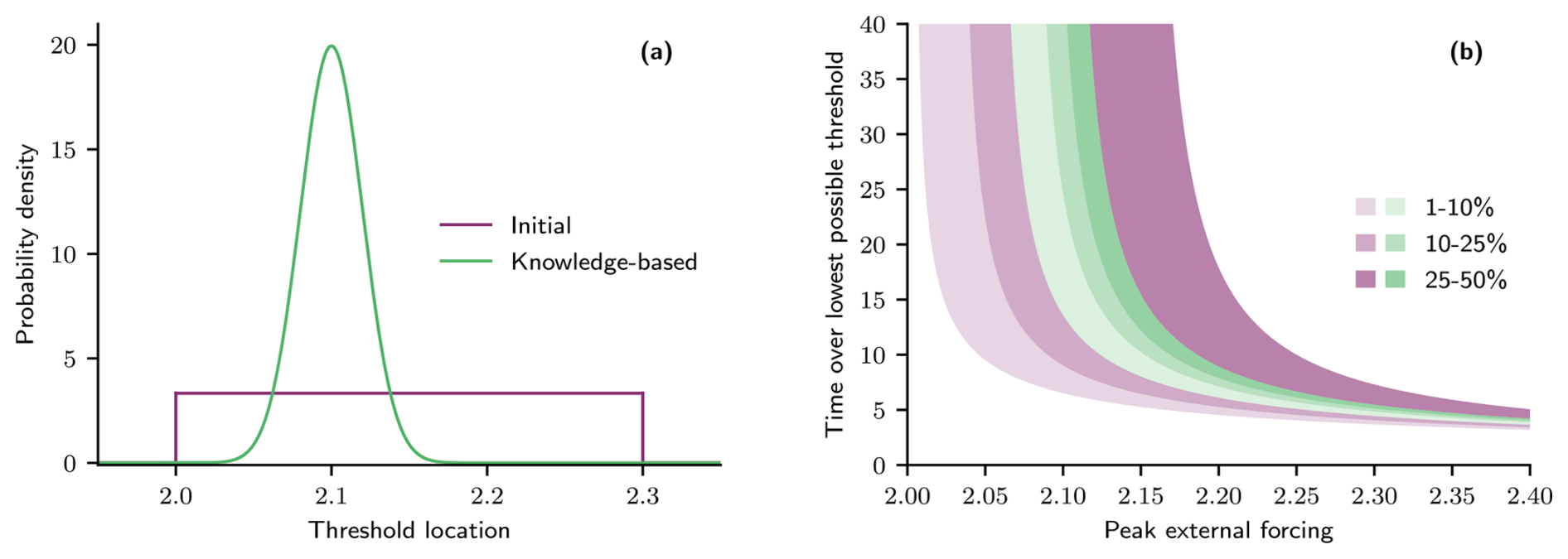
Figure 2 Constraining uncertainty in threshold location minimizes uncertainty in tipping behaviour for overshoot scenarios. (a) Probability distribution functions for threshold location, p_b. A uniform distribution, $p_b\sim \mathcal{U}[\mathrm{2.0},\mathrm{2.3}]$, is used as the initial distribution (purple), whereas the knowledge-based distribution is assumed to take the form of a normal distribution, $p_b\sim \mathcal{N}(\mathrm{2.1},{\mathrm{0.02}}^{\mathrm{2}})$ (green). (b) Theoretical tipping probability contours for overshoots characterized by the time over the lowest threshold (p_thr=2) and peak external forcing are given in colours corresponding to the distributions given in panel (a).

3.2 Uncertain linear restoring force

The previous section highlights how uncertainty in the location of the tipping threshold can affect the probability of tipping. Another important system characteristic for determining the mitigation window for overshoots is the strength of the linear restoring force. In this section, we again use the prototypical fold model Eq. (2) but keep the tipping threshold location fixed (p_b=2) and instead consider different linear restoring force proportionality factors κ.

Figure 3a provides an exemplary overshoot trajectory, as given by Eq. (3), which starts below the tipping threshold (indicated by the dotted red line) and then increases such that there is a brief overshoot before reversing the forcing back to its original level. Similarly to before, we can observe contrasting tipping behaviours for systems that differ only by the strength of the linear restoring force proportionality factor; see Fig. 3b. Namely, if the system has a weak linear restoring force (κ=1), the system does not undergo tipping (thin and opaque blue curve), whereas, if the restoring force is too strong, tipping cannot be prevented. The example given by the thick and translucent curves nearly recovers but does not cross the unstable branch (representing the boundary of the basin of attraction) when reducing the external forcing and so ultimately tips due to the restoring force being too strong (κ=2). The system with the weaker linear restoring force has a weaker “pull” towards the stable branch at which the system starts and therefore lags further behind the equilibrium of the static system than that of the system with the stronger restoring force. Consequently, when the system is forced beyond the critical threshold, the system with the weak restoring force will be slower to react once beyond the threshold and take longer to run away to an alternative state. In addition, for a weaker restoring force proportionality factor, the boundary of the basin of attraction (dashed black curve) is further away from the stable state (solid black curve in Fig. 3b). Therefore, the system with weak restoring force (thin and opaque dashed black curve) can cross the basin boundary at lower system state values compared to the system with a strong restoring force (thick and translucent dashed black curve). All these factors culminate in the system with strong restoring force tipping and the system with weak restoring force not tipping for the same forcing overshoot profile.

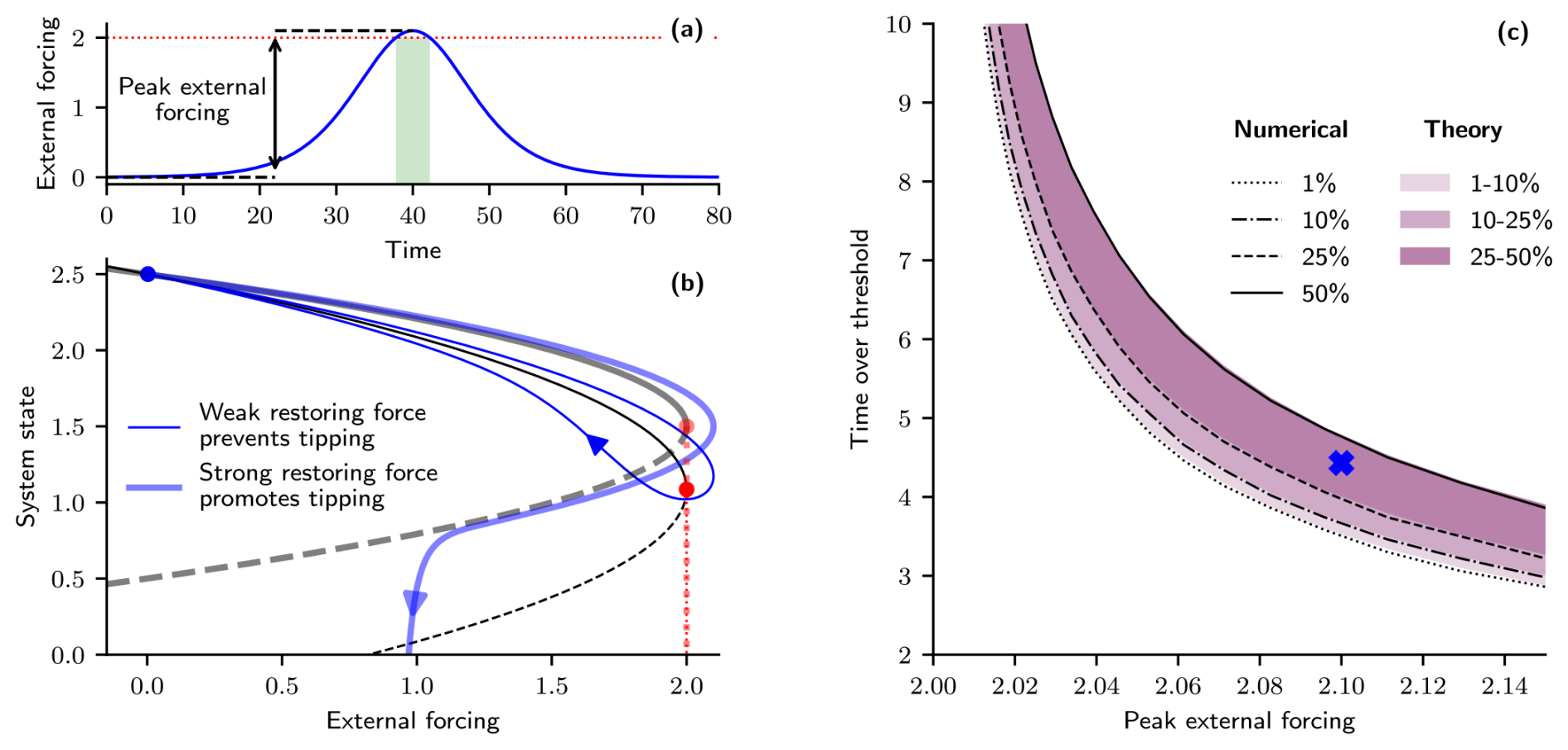
Figure 3 Probabilistic overshoots given uncertainty in the strength of the linear restoring force. (a) Time profile of an exemplary external forcing given by Eq. (3) (parameters: Δ_p=2.1, r=0.1, t_peak=40). The dotted red line indicates the tipping threshold location (p_b=2). (b) System responses (blue) subjected to the external forcing profile given in panel (a) for the model given by Eq. (2) with fixed p_b=2 but either with weak restoring force, κ=1 (thin and opaque), or strong restoring force, κ=2 (thick and translucent curves). Steady states indicated by black curves are either stable (solid) or unstable (dashed). Red opaque and translucent dots indicate the threshold location (fold bifurcation) of the respective systems. (c) Tipping probability contours for overshoots characterized by the time over the threshold (p_b=2) and peak forcing amplitude, given a uniform distribution in the restoring force proportionality factor, $\mathit{\kappa }\sim \mathcal{U}[\mathrm{0.25},\mathrm{3.25}]$. The purple colour gradient shows different probability boundary levels derived from the theory, Eq. (1). Black curves provide the probability levels calculated numerically. The blue cross corresponds to the time profile of external forcing given in panel (a), with the time over the threshold represented by the green shading and the peak in external forcing represented by the black arrow and dashed line.

Following a similar approach to before, we can consider a range of restoring force proportionality parameter values that are uniformly distributed, $\mathit{\kappa }\sim \mathcal{U}[\mathrm{0.25},\mathrm{3.25}]$. For any given overshoot profile, according to Eq. (3), the critical κ can be determined, and, with this, the probability of tipping equates to the proportion of the parameter distribution that is above this critical value. Figure 3c shows the probability of tipping for a range of overshoot profiles, characterized by the time over the threshold (which is now fixed, in contrast to Sect. 3.1) and the peak external forcing. The numerically calculated curves again display a very good agreement with the theory, especially for small and long overshoots. The blue cross corresponds to the particular overshoot profile given in panel (a), where the time over the threshold is indicated by the green shading and the peak external forcing is indicated by the black arrow and dashed lines.

Recall that, for small peak external forcing levels, the uncertainty in the tipping probability was large for uncertain tipping thresholds. In comparison, for uncertain restoring forces, the tipping uncertainty is substantially smaller (compare Figs. 1c and 3c). For a given trajectory, if the threshold is uncertain, then there may be no overshoot of the threshold, meaning the time to reverse the forcing is irrelevant given tipping is not possible (without noise). In contrast, if only the restoring force is uncertain, then it is known if the trajectory overshoots the threshold. Therefore, if it does overshoot, only a limited time can be spent over the threshold before tipping ensues.

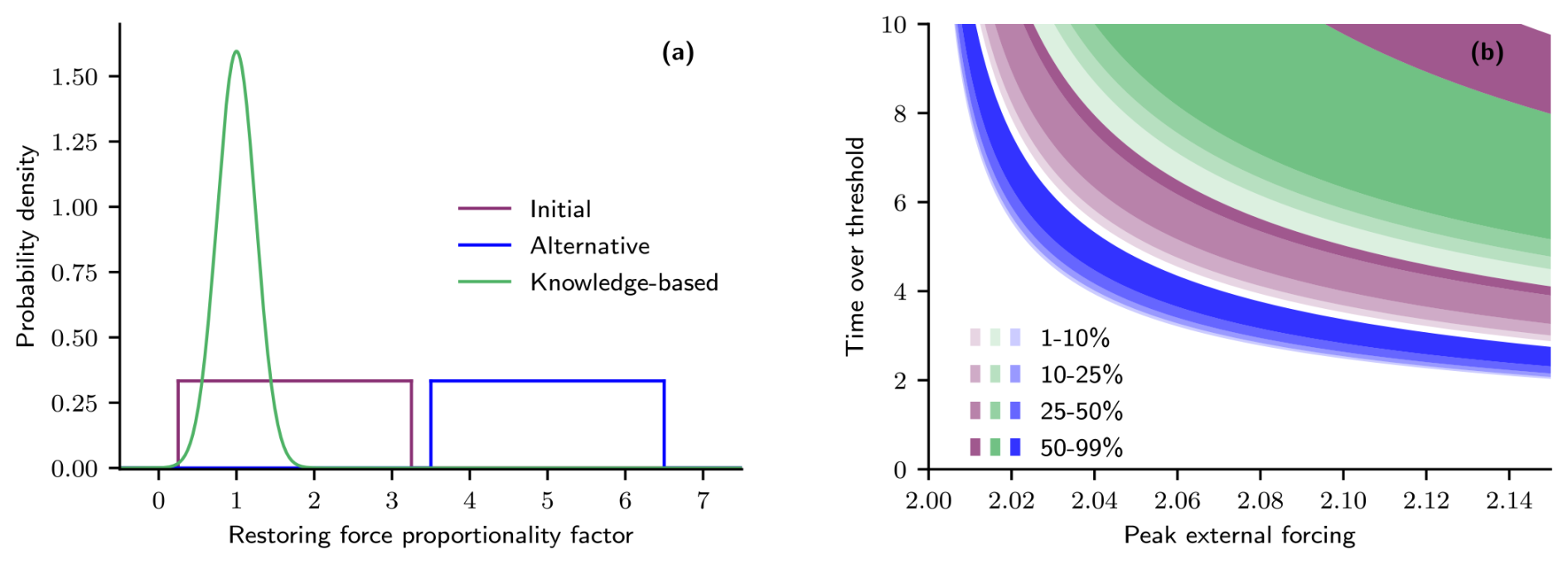
Figure 4 Constraining uncertainty in the linear restoring force reduces uncertainty in tipping behaviour for overshoot scenarios. (a) Probability distribution functions for the restoring force proportionality factor, κ. A uniform distribution, $\mathit{\kappa }\sim \mathcal{U}[\mathrm{0.25},\mathrm{3.25}]$, is used as the initial distribution (purple), whereas the knowledge-based distribution is assumed to take the form of a normal distribution, $\mathit{\kappa }\sim \mathcal{N}(\mathrm{1},{\mathrm{0.25}}^{\mathrm{2}})$ (green). An alternative initial uniform distribution, $\mathit{\kappa }\sim \mathcal{U}[\mathrm{3.5},\mathrm{6.5}]$ (blue), is also considered for same range of restoring force values but larger. (b) Theoretical tipping probability contours for overshoots characterized by the time over the threshold (p_b=2) and the peak external forcing are given in colours corresponding to the distributions given in panel (a).

Figure 4 shows how changing the uncertainty in the restoring force affects the tipping probability contours and therefore the uncertainty in tipping behaviour.

In Fig. 4a, we again start with an initial uniform distribution for the restoring proportionality factor, i.e. $\mathit{\kappa }\sim \mathcal{U}[\mathrm{0.25},\mathrm{3.25}]$ (purple), and assume that the knowledge-based distribution narrows down this uncertainty. We assume a normal distribution with a mean of 1 and a standard deviation of 0.25; i.e. $\mathit{\kappa }\sim \mathcal{N}(\mathrm{1},{\mathrm{0.25}}^{\mathrm{2}})$ (green).

The curves for the different probability levels of tipping shift substantially; see Fig. 4b. An overshoot trajectory that sits on the 50 % probability of tipping curve based on the initial distribution would be considered to be exceptionally unlikely (< 1 %) to cause tipping, given the knowledge-based distribution.

However, unlike for the threshold location, the distance (both horizontally and vertically) between the 1 % and 50 % tipping probability curves for the initial and knowledge-based distributions of the restoring force proportionality factor has barely changed. This seemingly counter-intuitive result can be explained by the change in the mean of the restoring force proportionality factor distribution counteracting the decrease in parameter uncertainty. To illustrate this, we consider an alternative uniform distribution, $\mathit{\kappa }\sim \mathcal{U}[\mathrm{3.5},\mathrm{6.5}]$ (blue), which is of the same width but has a much higher mean for the restoring force proportionality factor; see Fig. 4a. The distance between the 1 % and 50 % probability levels in Fig. 4b is much smaller for this alternative uniform distribution than for the initial uniform distribution. This illustrates that an uncertainty in the restoring force for large values is less critical than at lower values. Thus, when transitioning from the initial uniform distribution to the knowledge-based distribution, the reduction in parameter uncertainty would narrow the distance between the 1 % and 50 % probability contours but, by decreasing the mean, would simultaneously also widen the distance. So, for this example, little change in the distance between the 1 % and 50 % probability contours is observed. Importantly, though, the uncertainty of the location of the critical boundary (separating tipping from not tipping) does still decrease. This can be seen when plotting the 99 % probability of the tipping boundary and noticing that the separation between the 1 % and 99 % boundaries does indeed reduce.

So far, we have illustrated the effects of uncertainty in the tipping threshold location and the linear restoring force separately. We now come to a joint analysis of uncertainty by considering uncertainty in a model parameter for a simple conceptual model of the Atlantic Meridional Overturning Circulation (AMOC). The uncertainty stems from the diffusive timescale parameter that jointly influences the location of the tipping threshold and the linear restoring force.

4 Uncertain diffusive timescale in the Stommel–Cessi model

In this section, we consider how diffusive timescale uncertainties in a low-dimensional box model for the AMOC affect the uncertainty in tipping behaviour (i.e. if the AMOC collapses or not) for overshoot profiles of the freshwater flux into the North Atlantic.

The model, introduced by Cessi (1994), is a modification of the two-box Stommel model (Stommel, 1961) and describes the change in the non-dimensional meridional salinity gradient, x, which is a proxy for the strength of the AMOC:

$$\begin{array}{}\text{(5)}& {\displaystyle \frac{\mathrm{d}x}{\mathrm{d}s}}=p\left(s\right)-x(\mathrm{1}+{\mathit{\eta }}^{\mathrm{2}}(\mathrm{1}-x{)}^{\mathrm{2}}),\end{array}$$

where the parameter, ${\mathit{\eta }}^{\mathrm{2}}=t_{\mathrm{d}}/t_{\mathrm{a}}$, defines the ratio of the diffusive (t_d) to advective (t_a) timescales and s is a time parameter. If the freshwater flux, p(s), added to the North Atlantic becomes too large, it is possible to exceed a critical threshold, represented by a fold bifurcation in the model. This would cause the AMOC to tip from its current “on state” to a collapsed state, if exceeded for too long. Previously, Lux et al. (2022) showed how the location of this critical non-dimensional freshwater flux (along with the restoring force) changes upon varying the ratio of the diffusive (mixing by wind-driven gyres and eddies) to advective timescales. Specifically, the freshwater flux tipping threshold for AMOC collapse moves to lower values for smaller η². However, the scaling from the non-dimensional, p, to dimensional, $\stackrel{\mathrm{̃}}{F}$ (in m yr⁻¹), freshwater flux depends on the diffusive timescale:

$$\begin{array}{}\text{(6)}& \stackrel{\mathrm{̃}}{F}={\displaystyle \frac{{\mathit{\alpha }}_T\mathit{\theta }H}{{\mathit{\alpha }}_S{S}_{\mathrm{0}}{t}_{\mathrm{d}}}}p={\displaystyle \frac{\mathit{\xi }}{t_{\mathrm{d}}}}p,\end{array}$$

where a description of the parameters and their values can be found in the Appendix in Table A1. Therefore, how the ratio, η², is changed (i.e. by changing the diffusive and/or the advective timescale) will affect how the tipping threshold in the dimensional freshwater flux changes. In the next subsection, we present numerical investigations for the interplay between changing t_d versus t_a, which will motivate our choice for considering uncertainties in the diffusive timescale.

4.1 Joint influence of uncertain tipping threshold and uncertain linear restoring force

Figure 5 shows how the location of the dimensional critical freshwater fluxes (i.e. both the threshold indicating the transition to the collapsed off state and the threshold representing recovery back to the on state) and the width of the corresponding region of bistability (all denoted by colour) change with varying the advective and diffusive timescales. The black lines provide contours of constant ratio between the diffusive and advective timescales. A sufficiently large ratio between the diffusive and advective timescales is required for the AMOC to possess tipping behaviour (presence of critical thresholds for AMOC collapse, AMOC recovery, and a corresponding region of bistability). Hence, below this critical ratio (η²=3), the region is coloured white.

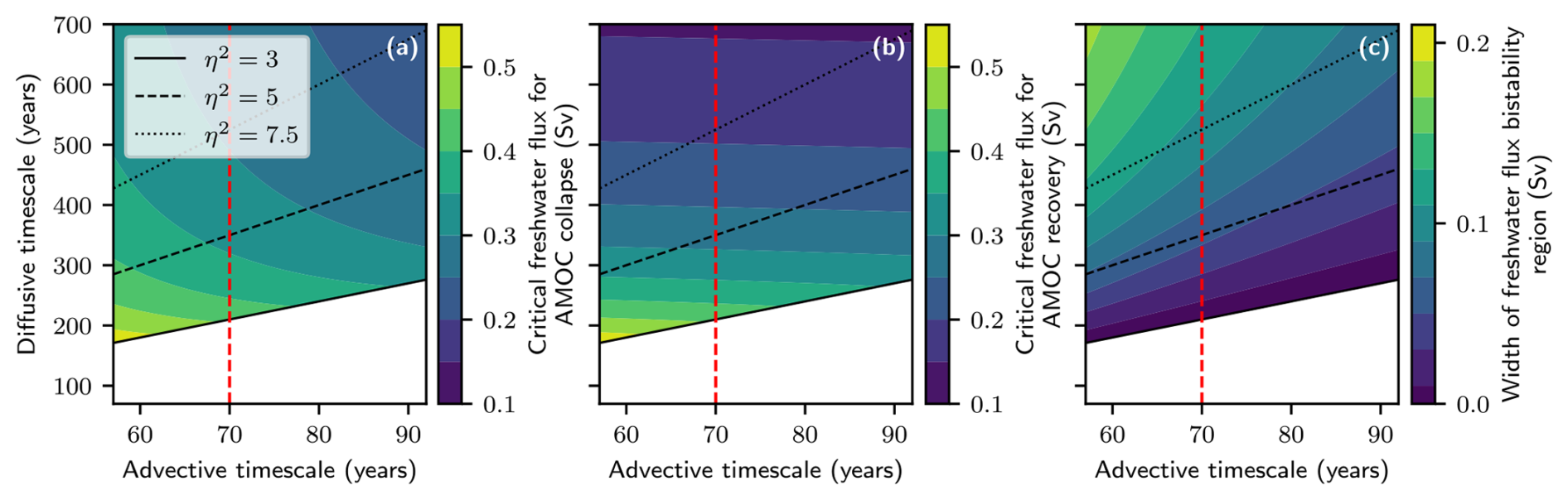
Figure 5 Critical freshwater fluxes and width of bistability region depending on advective and diffusive timescales. Colour plots for the location of the critical freshwater fluxes and the bistability region depending on the advective and diffusive timescales. (a) Location of the critical freshwater flux that triggers an AMOC collapse from the AMOC on state to the AMOC off state. (b) Location of the critical freshwater flux that triggers AMOC recovery from the off to the on state. (c) Width of bistability region, defined by the difference between the two critical freshwater fluxes. The region plotted corresponds to plausible advective and diffusive timescales as identified by Wood et al. (2019). Black lines are contours of the constant ratio between advective and diffusive timescales. The dashed red line denotes the value at which the advective timescale is fixed for analysis of an uncertain diffusive timescale.

Figure 5a shows the critical level of freshwater flux (denoted by colour) at which the AMOC on state terminates at a fold. Previously, it was shown that the critical non-dimensional freshwater flux only depends on the ratio of timescales and that decreasing this ratio (either by decreasing the diffusive timescale or increasing the advective timescale) moves the threshold to lower values (Lux et al., 2022). However, the scaling from a dimensional to a non-dimensional freshwater flux, introduced by Cessi (1994) and given in Eq. (6), depends on the diffusive timescale. Hence, the tipping threshold for the dimensional freshwater flux no longer remains constant along the contours of constant ratio. Instead, the tipping threshold in the dimensional freshwater flux moves to lower values for increasing either the advective timescale or the diffusive timescale.

Similarly, the scaling dependency, Eq. (6), affects the location of the other fold bifurcation/threshold corresponding to the termination of the off state; see Fig. 5b. Lux et al. (2022) found that the freshwater flux threshold representing the transition from AMOC off to AMOC on was largely constant and independent of the ratio of timescales. Hence, for dimensional quantities, this translates to the AMOC recovery threshold being independent of the advective timescale (i.e. for a fixed diffusive timescale, the threshold changes very little). On the other hand, the threshold decreases for increasing diffusive timescales, making it harder to restore the AMOC if it were to collapse.

The final panel, Fig. 5c, combines the first two panels by plotting in colour the difference between the two thresholds corresponding to the width of the region of bistability. Decreasing the diffusive timescale but keeping the advective timescale fixed decreases the width of bistability. Concurrently, both critical thresholds move to higher values, so these factors alone will make tipping less likely for any given overshoot. Additionally, the freshwater flux can be stabilized at a higher level, such that only the AMOC on state exists (since the threshold for AMOC recovery moves higher).

The chosen ranges of the advective and diffusive timescales correspond to the plausible ranges for the two different timescales, as determined by Wood et al. (2019). The advective timescale is relatively well constrained, whereas the uncertainty in the diffusive timescale is much larger. Consequently, we choose to fix the advective timescale (70 years, indicated by the dashed red line) within the physical range given in Lux et al. (2022), and instead we will now focus on the uncertainty in the diffusive timescale. Note that the scaling between the dimensional and non-dimensional freshwater flux in Eq. (6) (and the scaling of time) depends on the diffusive timescale. Therefore, the same non-dimensional freshwater flux time profile will translate into different dimensional time profiles for different diffusive timescales. This is the reason why we instead rescale time with respect to the advective timescale only, which changes Eq. (5) to

$$\begin{array}{}\text{(7)}& \dot{x}=p\left(t\right)-{\displaystyle \frac{x}{t_{\mathrm{d}}}}(t_{\mathrm{a}}+t_{\mathrm{d}}(\mathrm{1}-x{)}^{\mathrm{2}}),\end{array}$$

where the scalings to the dimensional quantities, salinity difference (ΔS [psu]), time (t^′ [years]), and freshwater flux (F now measured in Sverdrups [Sv]), are now given by

$$\begin{array}{}\text{(8)}& \mathrm{\Delta }S={\displaystyle \frac{{\mathit{\alpha }}_T\mathit{\theta }}{{\mathit{\alpha }}_S}}x,t^{\prime }=t_{a}t,F={\displaystyle \frac{{\mathit{\alpha }}_T\mathit{\theta }{V}_{\mathrm{0}}\mathit{\gamma }}{{\mathit{\alpha }}_S{S}_{\mathrm{0}}\mathit{\beta }{t}_{\mathrm{a}}}}p,\end{array}$$

where, again, a description of the parameters and their values can be found in the Appendix in Table A1. The dimensional AMOC flow strength, $Q(x,t_{\mathrm{d}},V)$, with units [Sv], is given by

$$\begin{array}{}\text{(9)}& Q(x,t_{\mathrm{d}},V)={\displaystyle \frac{\mathit{\gamma }V}{\mathit{\beta }{t}_a{t}_d}}(t_{\mathrm{a}}+t_{\mathrm{d}}(\mathrm{1}-x{)}^{\mathrm{2}}),\end{array}$$

where the ocean volume, V, is chosen such that the initial AMOC strength is equal to $Q_{\mathrm{0}}=Q(\mathrm{0},\mathrm{525},V_{\mathrm{0}})$. The reference volume V₀, given in Table A1, is an approximate value for the ocean volume based on general circulation models (Wood et al., 2019).

4.2 Uncertain diffusive timescale

We continue with analysing the AMOC tipping behaviour in the style of Figs. 1 and 3. Rather than using symmetric freshwater overshoot profiles (as before), in Fig. 6, we use more realistic profiles, first introduced by Huntingford et al. (2017), which take the form

$$\begin{array}{}\text{(10)}& p\left(t\right)=p_{\mathrm{0}}+\mathit{\gamma }t-(\mathrm{1}-\exp (-\mathit{\mu }\left(t\right)t\left)\right)(\mathit{\gamma }t-(p_{\mathrm{stab}}-p_{\mathrm{0}}\left)\right).\end{array}$$

Equation (10) allows the flexibility to start and finish at different levels (p₀=0, $p_{\mathrm{stab}}=t_{\mathrm{a}}/\mathit{\xi }$, which equates to stabilizing at just below 0.25 Sv). The stabilization level (p_stab) is chosen such that the freshwater always stabilizes below the critical threshold for AMOC collapse but above the threshold for AMOC recovery in most cases. The transition between the initial level and the stabilization level is determined by $\mathit{\mu }\left(t\right)={\mathit{\mu }}_{\mathrm{0}}+{\mathit{\mu }}_{\mathrm{1}}t$, where μ₀ and μ₁ determine the maximum amplitude and time to converge to the stabilization level. The parameter $\mathit{\gamma }=r-{\mathit{\mu }}_{\mathrm{0}}(p_{\mathrm{stab}}-p_{\mathrm{0}})$ is chosen to ensure that all profiles have the same initial rate of increase, determined by r=0.01.

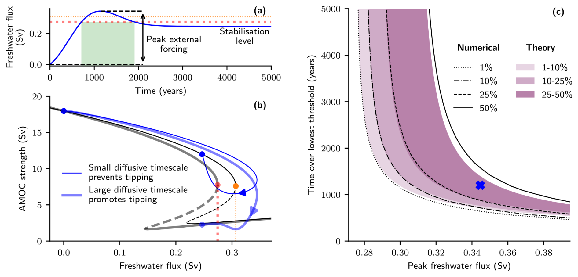
Figure 6 Probabilistic overshoots given uncertainty in the diffusive timescale of the AMOC Stommel–Cessi model. (a) Time profile of an exemplary freshwater flux given by Eq. (10) (parameters: p₀=0, $p_{lim}=\mathrm{1}/\mathit{\xi }$, ${\mathit{\mu }}_{\mathrm{0}}=-\mathrm{0.05}$, μ₁=0.0057, r=0.01). The red and dotted lines indicate thresholds corresponding to large (t_d=700) and small (t_d=455) diffusive timescales respectively. (b) System responses (blue) subjected to the freshwater flux profile given in panel (a) for the model given by Eq. (7) and the AMOC strength expressed by Eq. (9) for either a small diffusive timescale, t_d=455 (thin and opaque curves), or a large diffusive timescale, t_d=700 (thick and translucent curves). Further system parameter values can be found in Table A1. Steady states, indicated by black curves, are either stable (solid) or unstable (dashed). Orange and red dots indicate threshold locations (fold bifurcations) of the respective systems. (c) Tipping probability contours for overshoots characterized by the time over the lowest threshold (corresponding to a diffusive timescale of 700 years) and peak forcing amplitude, given a uniform distribution in the diffusive timescale, $t_{\mathrm{d}}\sim \mathcal{U}[\mathrm{210},\mathrm{700}]$. The purple colour gradient shows different probability mass levels derived from the theory, Eq. (4). The blue cross corresponds to the time profile of freshwater flux given in panel (a), with the time over the lowest threshold represented by the green shading and the peak in external forcing represented by the black arrow and dashed line.

Following a similar approach to before, we investigate the effect of uncertainty in the diffusive timescale on the overshoots and the mitigation window. For the exemplary overshoot trajectory given in Fig. 6a, the system's response is shown for both a small (t_d=455 years, thin and opaque curves) and a large (t_d=700 years, thick and translucent curves) diffusive timescale but for a fixed advective timescale (t_a=70 years) in Fig. 6b. In the case of a small diffusive timescale, the tipping threshold would be far away (dotted orange lines), so the overshoot would be small and for a short duration of time. Note also that the bistability region is small for small diffusive timescales; therefore, in this example (t_d=455), the AMOC would recover (regardless of the overshoot time) if the freshwater flux was reduced back to below the lower fold at approximately 0.22 Sv.

In contrast, if the diffusive timescale is large, then the AMOC would collapse and not recover. This is by virtue of the threshold being a lot lower (dotted red lines) causing the overshoot of the tipping threshold to be much larger and for a longer period of time. These combined factors, coupled with a larger bistability region (stabilizing within the bistability region), mean that the AMOC tips to its off state.

In Fig. 6c, we consider all plausible diffusive timescales (that also provide a region of bistability) with equal likelihood ($t_{\mathrm{d}}\sim \mathcal{U}[\mathrm{210},\mathrm{700}]$) and plot the probability of tipping for overshoot profiles of the form given by Eq. (10). The overshoots are again characterized by the duration of time that the freshwater flux is above the lowest threshold (corresponding to a diffusive timescale of 700 years) and by the peak freshwater flux indicated by the green shaded region and black arrow respectively in Fig. 6a. For sufficiently small diffusive timescales, recovery to the AMOC on state is guaranteed even if the AMOC temporarily collapses. This is a result of the freshwater flux stabilizing below the bistability region, where the on state is the only stable equilibrium. For the uniform prior distribution, there is just under a 40 % probability that the freshwater flux stabilizes below the bistability region (but never above, which would guarantee tipping). Hence, we cannot rule out the possibility of AMOC recovery even for very large and long overshoots.

A good correlation is once again found between the inverse-square law theory, Eq. (4), and the numerically calculated probability boundaries, particularly for the smaller peak freshwater overshoots. However, for larger overshoots, discrepancies arise between the numerics and theory. At the 1 % level, the theory overestimates the critical boundary, caused by the asymmetry of the forcing profile. However, at the 50 % level, the theory underestimates the critical boundary. The shrinking region of bistability (i.e. due to the presence of another fold bifurcation) and the initializing of simulations in equilibrium provide additional sources of error. Specifically, strongly forced systems are not in equilibrium. Therefore, making the assumption that the AMOC is in equilibrium at the start of the simulation will cause an overestimation of the numerical probability of tipping, particularly for tipping thresholds that are close.

The large uncertainty in the system parameter, here in terms of the diffusive timescale, again causes large uncertainties in the tipping behaviour. Therefore, it is necessary to constrain the uncertainty in the diffusive timescale to reduce the uncertainty in the tipping behaviour. The approach we use to constrain the uncertainty in the diffusive timescale is through Bayesian inference (Stuart, 2010). The procedure is analogous to the one used in Lux et al. (2022), especially in terms of the discrepancy model, the likelihood function, and the generation of the synthetic time series. Note that we use synthetically generated data due to the absence of real-world data for the AMOC to be matched to the Stommel–Cessi box model. We assume a true value for the diffusive timescale parameter t_d=525 years, and the underlying ODE is given by Eq. (7). We use a Markov chain Monte Carlo (MCMC) approach (Brooks et al., 2011), where the idea is to obtain the desired data-informed (posterior) distribution as the invariant distribution of the Markov chain over the prior support. We obtain the posterior distribution by running an MCMC algorithm provided in the MATLAB-based software framework UQLab (Marelli and Sudret, 2014), version 1.3.0, using the affine invariant ensemble sampler with 100 Markov chains with 400 steps (see the manual (Wagner et al., 2022) for a detailed documentation).

Performing Bayesian inference starting with the uniform prior distribution (purple), we are able to create a tightly constrained posterior distribution (green) centred close to the assumed diffusive timescale of 525 years; see Fig. 7a.

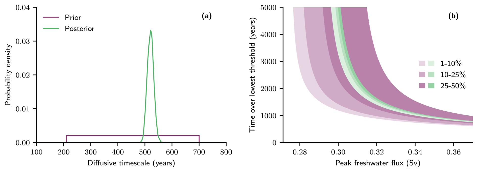
Figure 7 Constraining uncertainty in the diffusive timescale minimizes uncertainty in tipping behaviour for overshoot scenarios. (a) Probability distribution functions for diffusive timescale, t_d. A uniform distribution, $t_{\mathrm{d}}\sim \mathcal{U}[\mathrm{210},\mathrm{700}]$, is used as a prior distribution (purple), whereas the posterior distribution has been calculated by performing Bayesian inference on synthetic data generated for an assumed diffusive timescale of 525 years (green). (b) Theoretical tipping probability contours for overshoots characterized by the time over the lowest possible threshold (given the prior distribution) and peak freshwater flux amplitude are given in colours corresponding to the distributions given in panel (a).

The tightly constrained posterior distribution of the diffusive timescale results in a strong reduction in the uncertainty of the mitigation window; see comparison of purple to green in Fig. 7b. An overshoot that has a 25 % probability of tipping, based on the prior distribution, would be classified as exceptionally unlikely with less than 1 % probability of tipping given the posterior distribution. Furthermore, as can be inferred from Fig. 5b, the stabilization level is within the bistability region (more than 99 % confidence). Note that the critical freshwater flux threshold for AMOC recovery is only below the stabilization level for diffusive timescales greater than 400 years. Thus, for the posterior distribution, the time taken to reverse the freshwater flux is critical to determine whether tipping occurs or not, whereas, previously, the prior distribution included timescale values that yielded critical thresholds for AMOC recovery higher than the stabilization level of the freshwater flux. Therefore, the probability for AMOC recovery would be non-zero regardless of the time taken to reverse the freshwater flux.

While the analysis in Fig. 7b covers a whole spectrum of different overshoot trajectories, Fig. 8 performs a more in-depth analysis of how the probability of tipping for a single overshoot trajectory changes based on the distribution of the diffusive timescale. A zoomed-in view of the overshoot trajectory is given in Fig. 8a. For any overshoot, there exists a critical diffusive timescale such that smaller diffusive timescales will prevent the AMOC from collapsing. The tipping threshold that corresponds to this critical diffusive timescale (for the particular overshoot given) is plotted in black. If the diffusive timescale is smaller, the tipping threshold will be higher, meaning that the overshoot of the threshold will be smaller and for a shorter duration (compare orange line with black line). Let us now consider some uncertainty on the diffusive timescale, centred around a reference value $t_{\mathrm{d}}^{\text{ref}}=$ 450 years that corresponds to the orange threshold $p_b^{\text{ref}}=$ 0.308 Sv. The orange banding represents the threshold locations p_b that arise from a nonlinear transformation of t_d within 1 standard deviation (125 years) of $t_{\mathrm{d}}^{\text{ref}}$. Note that the nonlinear relation between the diffusive timescale parameter and the threshold location makes the orange band not symmetrically distributed around the orange line. Despite an assumed normal distribution on the diffusive timescale, the distribution of thresholds is not normally distributed. Visibly, within 1 standard deviation of the mean includes both timescales above the critical level that would cause the AMOC to tip and timescales that would avoid the system crossing the threshold altogether for the same overshoot trajectory.

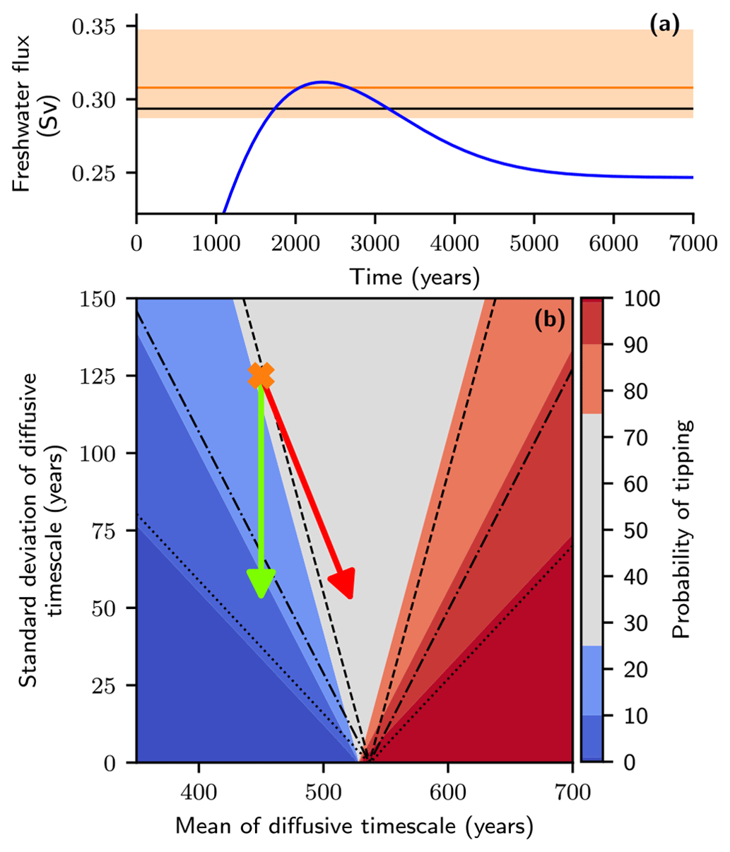
Figure 8 Probability of avoiding tipping for a single overshoot trajectory based on diffusive timescale distribution. (a) Time profile of an exemplary overshoot trajectory (zoomed in) given by Eq. (10) (parameters: p₀=0, $p_{lim}=\mathrm{1}/\mathit{\xi }$, μ₀=0.005, μ₁=0.0009, r=0.01) (Huntingford et al., 2017). The black horizontal line provides the location of the tipping threshold at the critical diffusive timescale separating tipping from not tipping. The orange line (mean) and banding (mean ±1 standard deviation) show the location of the critical threshold for a diffusive timescale parameter distribution that is normally distributed with a mean of 450 years and a standard deviation of 125 years (denoted by orange cross in panel (b)). (b) Plot of the probability of tipping for the overshoot given in panel (a) depending on the characteristics of a normally distributed diffusive timescale parameter. Colours give the sampling-based, numerically calculated probability of tipping, and black contours give the theoretical probability of tipping derived from the inverse-square law relationship given by Eq. (4).

In Fig. 8b, the probability of tipping is plotted based on the mean and standard deviation of the normally distributed diffusive timescale. The orange cross corresponds to the mean and standard deviation given in Fig. 8a. If the standard deviation of the distribution is 0 (i.e. the diffusive timescale is known), then, without stochastic variability in the system, the probability of tipping is either zero or 100 %. Increasing the standard deviation a little will create some tipping uncertainty close to the critical diffusive timescale for the specific trajectory, but still, for most of the cross-section, the probability of tipping will be close to zero or 100 %. As the standard deviation increases further, more distributions will include the critical diffusive timescale with some non-small probability and therefore create greater tipping uncertainty. Thus, the region of tipping uncertainty spreads out for increasing standard deviation as shown numerically by the colouring.

Figure 8b shows that, if the standard deviation is reduced but the mean of the diffusive timescale kept fixed (i.e. follow the green arrow), then the uncertainty in the tipping behaviour reduces (probability of tipping moves further away from 50 %). However, generally, when reducing parameter uncertainty (standard deviation), the mean will also likely change. In some scenarios, it is possible for the uncertainty in the tipping behaviour to increase despite a reduced uncertainty in the timescale. For example, if we instead follow the red arrow, then the probability of tipping changes from approximately 25 % to 50 %. However, here the orange line is moving down towards the black line, and, at the same time, the banding is shrinking around the orange line. Therefore, we are instead establishing that this particular overshoot is close to the critical overshoot that separates tipping from not tipping, but, importantly, if all possible overshoot trajectories are considered, then the overall uncertainty in the tipping behaviour will still reduce.

The theoretical contours are added to Fig. 8b as black lines of different line styles and show a good agreement to the numerically calculated probability given by the colour plot. The discrepancy arises from determining the value of the critical diffusive timescale. This is best identified on the x axis for 0 standard deviation, where the black contours converge at a diffusive timescale that is roughly 10 years longer than where the colours converge.

5 Conclusions

In this paper, we studied how uncertainty in model parameters can propagate to uncertainty in the tipping behaviour for systems subjected to overshoot trajectories. The location of the threshold and the linear restoring force are two key characteristics that were identified and in turn isolated to examine their importance for the possibility of avoiding tipping. Specifically, we have found that the tipping behaviour from a single overshoot scenario can completely change based solely on either the location of the tipping threshold or the strength of the linear restoring force.

Uncertainty in the location of the tipping threshold was the characteristic found to have the most influence on the uncertainty in the tipping behaviour. For a given overshoot trajectory, the threshold location will simply determine if an overshoot of the threshold occurs. Assuming an overshoot of the threshold does occur, both the peak overshoot distance and the time spent over the threshold would be smaller for a high threshold compared to a low threshold. These properties of the overshoot feature in the left-hand side of the inverse-square law, Eq. (1), while the right-hand side, interpreted as an upper bound for the mitigation window, remains fixed given a fixed linear restoring force. Constraining the uncertainty in the location of the tipping threshold will constrain the uncertainty in both the peak overshoot distance and duration of an overshoot and therefore considerably reduce the uncertainty in the tipping behaviour.

Another source of uncertainty can be in the strength of the linear restoring force to the stable equilibrium, which propagates into uncertainty in the upper bound for the mitigation window (the right-hand side of Eq. (1)). The linear restoring force features in the denominator of the right-hand side; therefore a weaker restoring force will help prevent tipping by increasing the upper bound for the mitigation window. This can be intuitively understood by a weaker restoring force causing a system to further lag its stable equilibrium (of the static system) under a change in external forcing. Therefore, reducing the uncertainty in the restoring force will reduce the uncertainty in the tipping delay from a system crossing its threshold and therefore how quickly the forcing needs to be reversed to prevent tipping.

We utilized a simple model for the Atlantic Meridional Overturning Circulation (AMOC) to demonstrate how uncertainty in the diffusive timescale parameter propagates simultaneously to uncertainty in the location of the threshold and the linear restoring force. Although the advective timescale is well constrained across climate models, a large uncertainty remains in the diffusive timescale. This ultimately results in uncertainty in the tipping behaviour for overshoot scenarios. For the AMOC, this translates to a large uncertainty in the probability of the AMOC collapsing.

Constraining parameter uncertainty, for instance, by performing Bayesian inference on observational data, can greatly reduce the uncertainty in the tipping behaviour. For a parameter distribution with a known cumulative distribution function, the probability of tipping can be efficiently calculated in terms of computational costs by using the inverse-square law relationship. This avoids a sampling-based approach. Techniques presented in this paper might carry over to overshoots in more complex AMOC models, such as the five-box AMOC model from Wood et al. (2019). For this AMOC model, instead of using synthetic data for the Bayesian inference procedure, it is possible to use box-averaged time series data of general circulation model runs, which puts the parameter inference on a more realistic base. Note, however, that a remaining challenge is to account for the presence of a Hopf bifurcation for some model parameter configurations, where tipping via the Hopf bifurcation (or rate-induced tipping) can occur before the system actually undergoes a fold bifurcation. An extension of the inverse-square law theory would be required, since it is currently designed to only consider overshoots of a fold bifurcation. Moreover, further research is required to understand how the theory can be applied to multiple uncertain parameters in more complex models.

Considering the added possibilities of tipping via other mechanisms can further change the conclusions. Note that the different mechanisms of tipping may also interact with each other: see the studies of Ritchie and Sieber (2017) and Slyman and Jones (2023) for the interplay between rate- and noise-induced tipping and of O'Keeffe and Wieczorek (2020) and Alkhayuon et al. (2019), for example, for the combination of rate- and bifurcation-induced tipping. For instance, if variability is considered (i.e. with the added possibility of noise-induced tipping), the longer a system spends close to or beyond the threshold, the easier it is for a system to be triggered into tipping (Ritchie et al., 2019). This further emphasizes that minimizing the duration of any overshoot of a tipping threshold is paramount to preventing tipping. Furthermore, if rate-induced tipping were possible, then multiple critical rates could arise for the same peak external forcing (Ritchie et al., 2023); therefore constraining system uncertainties becomes even more critical when considering overshoot scenarios.

Alternative profile shapes may also reduce the distinction between large but short and small but long overshoots (Enache et al., 2025). Moreover, uncertainties in the overshoot profile characteristics also need to be considered. For example, the precise peak overshoot distance and time spent over the tipping threshold are likely to be uncertain.

For a simple conceptual model of the AMOC, we find that, for any sized overshoot, provided the duration is less than 800 years, tipping would very likely be avoided. Importantly, this encompasses most policy-relevant overshoots under consideration (see e.g. Kikstra et al., 2022); therefore this low-dimensional box model would suggest AMOC tipping is very unlikely. However, it is important to note that these timescales are likely to be much longer than those observed in climate models (or the real world) (Jackson et al., 2023). Box models for the AMOC, such as that used for this study, tend to omit important advective responses that would otherwise make the response time faster (Jackson and Wood, 2018b).

Current rates of anthropogenic emissions make crossing climate tipping thresholds increasingly likely, despite us not knowing their exact location. This study revealed the strong influence of uncertainty in the location of the tipping threshold and the strength of the linear restoring force on the uncertainty in the tipping behaviour in response to possible overshoot trajectories. We have shown that constraining the uncertainty in these system characteristics enables us to better constrain the mitigation window, which is crucial to avoiding tipping elements of the climate system under overshoot scenarios.

Appendix A: Methods

A1 Overshoot theory for arbitrary threshold

The overshoot theory, as given by Eq. (1), details the time allowed over the tipping threshold. However, if the threshold location is uncertain, we would like to generalize this to the time over an arbitrary threshold, p_thr; in our case, we use the lowest tipping threshold according to the initial distribution. We follow a similar approach used in the original derivation in Ritchie et al. (2019), starting with the overshoot theory given by

$$\begin{array}{}\text{(A1)}& p_{\mathrm{peak}}-p_b<{\displaystyle \frac{\mathrm{1}}{a_{\mathrm{0}}}}\sqrt{-{\displaystyle \frac{\ddot{p}\left(t_{\mathrm{peak}}\right)}{\mathrm{2}\mathit{\kappa }}}}.\end{array}$$

The Taylor expansion of the forcing profile, p(t), about the peak level of forcing p_peak at time t_peak, is given by

$$\begin{array}{}\text{(A2)}& p\left(t\right)\approx p_{\mathrm{peak}}+{\displaystyle \frac{\mathrm{1}}{\mathrm{2}}}\ddot{p}\left(t_{\mathrm{peak}}\right)(t-t_{\mathrm{peak}}{)}^{\mathrm{2}}.\end{array}$$

Using Eq. (A2), let us consider the time over, t_over,thr, a prescribed threshold, p_thr<p_peak:

$$\begin{array}{}\text{(A3)}& t_{\mathrm{over},\mathrm{thr}}=\mathrm{2}\sqrt{{\displaystyle \frac{\mathrm{2}(p_{\mathrm{peak}}-p_{\mathrm{thr}})}{-\ddot{p}\left(t_{\mathrm{peak}}\right)}}}.\end{array}$$

Rearranging Eq. (A3) for $\ddot{p}\left(t_{\mathrm{peak}}\right)$ and substituting into Eq. (A1) gives the expression for the time allowed over an arbitrary threshold

$$\begin{array}{}\text{(A4)}& t_{\mathrm{over},\mathrm{thr}}^{\mathrm{2}}<{\displaystyle \frac{\mathrm{4}(p_{\mathrm{peak}}-p_{\mathrm{thr}})}{a_{\mathrm{0}}^{\mathrm{2}}\mathit{\kappa }(p_{\mathrm{peak}}-p_b{)}^{\mathrm{2}}}},\end{array}$$

as given in the main text in Eq. (4). Importantly, if the threshold is chosen to be the tipping threshold (p_thr=p_b), then Eq. (A4) reduces to the original inverse-square law, Eq. (1).

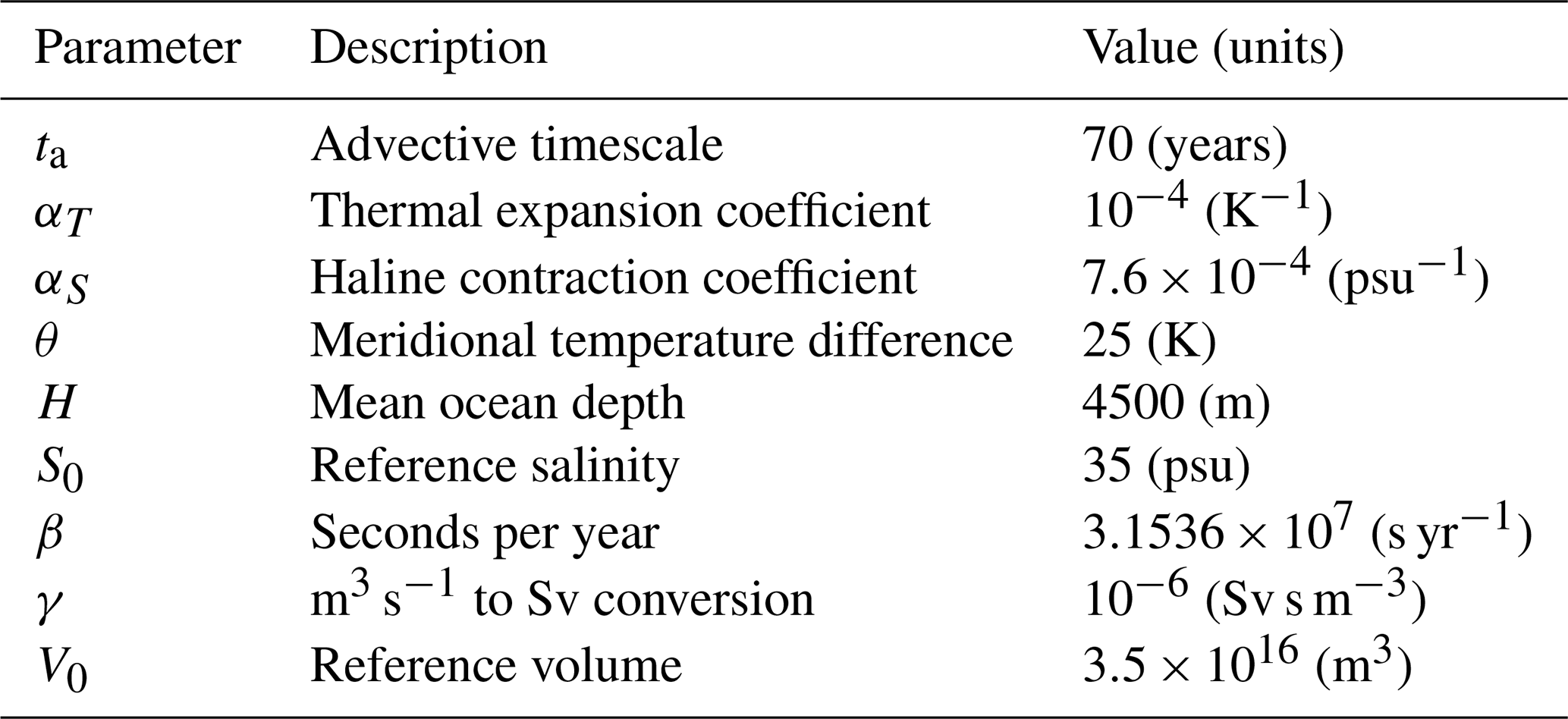
Table A1 Description of parameters and their values used in the Stommel–Cessi model.