Multi-million-year cycles in modelled δ¹³C as a response to astronomical forcing of organic matter fluxes

Along with 400 kyr periodicities, multi-million-year cycles have been found in δ¹³C records over different time periods. An ∼ 8–9 Myr periodicity is found throughout the Cenozoic and part of the Mesozoic. The robust presence of this periodicity in δ¹³C records suggests an astronomical origin. However, this periodicity is barely visible in the astronomical forcing. Due to the large fractionation factor of organic matter, its burial or oxidation produces large δ¹³C variations for moderate carbon variations. Therefore, astronomical forcing of organic matter fluxes is a plausible candidate to explain the oscillations observed in the δ¹³C records. So far, modelling studies forcing astronomically the organic matter burial have been able to produce 400 kyr and 2.4 Myr cycles in δ¹³C but were not able to produce longer cycles, such as 8–9 Myr cycles. Here, we propose a mathematical mechanism compatible with the biogeochemistry that could explain the presence of multi-million-year cycles in the δ¹³C records and their stability over time: a preferential phase locking to multiples of the 2.4 Myr eccentricity period. With a simple non-linear conceptual model for the carbon cycle that has multiple equilibria, we are able to extract longer periods than with a simple linear model – more specifically, multi-million-year periods.

1 Introduction

Astronomical frequencies are imprinted into the carbon cycle. A 400 kyr oscillation has been seen in many δ¹³C records covering the Cenozoic: during the Palaeocene (Westerhold et al., 2011), the Eocene (Lauretano et al., 2015), the Oligocene (Pälike et al., 2006), the Miocene (Billups et al., 2004), and during more recent time periods (Wang et al., 2010). The 400 kyr frequency corresponds to one of the frequencies of eccentricity, and this is the most stable astronomical periodicity through geological times (Laskar et al., 2004).

Longer cycles of 2.4 Myr have also been found in δ¹³C records over the Cenozoic: over the Oligocene (Pälike et al., 2006; Boulila et al., 2012) and Miocene (Liebrand et al., 2016). The 2.4 Myr periodicity is, at the same time, a true eccentricity cycle and present in the amplitude modulation (AM) of the 100 and 400 kyr cycles (Laskar et al., 2011; Boulila et al., 2012).

∼ 4.5 Myr cycles have also been observed in δ¹³C in the late Cretaceous (Sprovieri et al., 2013), as well as in the latest Ordovician and Silurian (Sproson, 2020).

Much longer and dominant cycles of approximately 9 Myr have been found in δ¹³C records over the Cenozoic (Boulila et al., 2012) and the Mesozoic (Martinez and Dera, 2015). Cycles of around 8 Myr have been seen in δ¹³C in the late Cretaceous (Sprovieri et al., 2013). This periodicity therefore seems very stable over time. The robust presence of ∼ 9 Myr cycles over various time periods hints at an astronomical origin. However, in the case of 4.5 and 9 Myr cycles, the link to the astronomical forcing is less clear, as these frequencies are not easily seen in the eccentricity spectra. A ∼ 4.5 Myr periodicity is visible in the eccentricity solution, although with a very low amplitude. The AM envelopes of the 100 and 400 kyr eccentricity also show a ∼ 4.5 Myr cyclicity but again with low amplitude. The ∼ 9 Myr frequency is not directly visible in the eccentricity spectra. Although it has been suggested that the AM envelope of the ∼ 2.4 Myr filtered eccentricity has a ∼ 9 Myr cyclicity (Boulila et al., 2012), this is with a very low amplitude. Therefore, the way in which the astronomy could pace these multi-million-year cycles remains mysterious.

It has been suggested (Paillard, 2017; Kocken et al., 2019) that an astronomical forcing of organic carbon fluxes could explain the observed δ¹³C cyclicities at 400 kyr and 2.4 Myr. Indeed, ¹²C-enriched organic matter burial or oxidation can lead to a relatively large δ¹³C variation for a moderate carbon variation, which is not possible with silicate weathering (Paillard, 2017; Russon et al., 2010). It is usually assumed that the long-term carbon cycle is mainly controlled by silicate weathering. But it is a negative feedback that does not allow for oscillatory behaviour as observed in the data. Additionally, recent studies have highlighted the important role played by organic carbon fluxes in the long-term carbon budget, acting as either a source if petrogenic organic carbon is eroded and oxidized or as a sink if terrestrial organic carbon is exported and buried into sediments (Hilton and West, 2020). Organic carbon contributions are of the same order of magnitude as silicate weathering (Hilton and West, 2020). Therefore, astronomical forcing of the organic matter burial is a plausible candidate to explain the observed cyclic δ¹³C variations.

Kocken et al. (2019) suggested that the link between δ¹³C and the astronomical forcing could be explained by enhanced marine organic carbon burial for lower eccentricity values. Periods of low eccentricity and therefore low seasonal contrast could favour annual wet conditions and, consequently, clay formation. The majority of organic carbon is buried in association with clay particles (Hedges and Keil, 1995). If transport is not limiting, lower eccentricity would lead to higher marine organic carbon burial and increased δ¹³C. Paillard (2017) suggested a link between monsoons and organic carbon burial. Monsoons favour soil erosion and sediment transports. Recent soil and petrogenic organic carbon can be eroded and carried to the oceans via rivers. The net effect on organic carbon burial depends on the geomorphological dynamics. For aggradational situations that favour burial, the net result is organic matter burial. In that case, δ¹³C increases with increased eccentricity and monsoon strength. However, for progradational situations, oxidation of petrogenic organic carbon is favoured, leading to a δ¹³C decrease with eccentricity increase. Martinez and Dera (2015) suggested that low eccentricity values and the associated stable and humid conditions could favour constant freshwater and nutrient inputs, thus favouring water mass stratification and productivity levels, leading to persistent anoxia and therefore higher organic carbon burial rates. On the contrary, high eccentricity values are associated with a recovery of oxic conditions during the cool season, limiting organic carbon burial. It has also been suggested that terrestrial organic carbon burial could increase with eccentricity minima, as this would favour annual soil anoxia (Kurtz et al., 2003). Laurin et al. (2015) suggested that δ¹³C variations in the Late Cretaceous could be explained by a transient storage of organic matter or methane in quasi-stable reservoirs such as wetlands, soils, marginal zones of marine euxinic strata, and permafrost. These quasi-stable reservoirs could respond non-linearly to changes in obliquity and the consequent high-latitude insolation changes or changes in meridional insolation gradients.

Other mechanisms have been proposed to explain δ¹³C variation as a consequence of astronomical variations; de Boer et al. (2014) suggested that ice sheet dynamics and linked changes in carbon cycle dynamics could explain the 400 kyr cycles in δ¹³C. However, this mechanism does not permit an explanation of the presence of such cycles for periods without ice sheets (Kocken et al., 2019).

Modelling studies forcing the net organic matter burial through eccentricity have been able to produce 400 kyr and 2.4 Myr cycles in the δ¹³C (Paillard, 2017; Kocken et al., 2019). However, these studies did not find longer cycles, such as the ∼ 4.5 and ∼ 9 Myr cycles observed in geological records. The models used were linear, and non-linear mechanisms might be necessary in order to produce multi-million-year cycles that have a very low amplitude in the input forcing.

Here, we develop a new conceptual model of the carbon cycle that includes a net organic matter burial term and force it astronomically with the eccentricity, similarly to the study of Paillard (2017). However, contrary to this study, the organic matter fluxes also depend on the surface carbon content with regard to its influence on climate and on atmospheric oxygen content. Our model therefore couples the carbon and oxygen cycles and is non-linear, with the possibility of multiple equilibria.

Our model is simple and is not designed to be a faithful representation of reality. Rather, we try to produce the simplest model possible that can produce results qualitatively, similarly to the carbon isotope record, while being compatible with biogeochemistry. This type of approach has been used by Bachan et al. (2017) for a different purpose: to explain δ¹³C excursions during the Mesozoic, having a duration of 0.5 to 10 Myr and a declining amplitude over time. Our model is not suited to representing specific excursions in δ¹³C due to particular events of organic matter burial. In this paper, we rather focus on the persistent multi-million-year cyclicity observed in δ¹³C over the last ∼ 200 Myr, over the Cenozoic and latest Mesozoic (Boulila et al., 2012; Martinez and Dera, 2015). With the model we have developed, it is possible to obtain multi-million-year frequencies in the δ¹³C. Depending on the strength of the astronomical forcing, periodicities of 2.4, ∼ 4.8, ∼ 7, and ∼ 9 Myr are produced preferentially, presumably as a result of phase locking to the 2.4 Myr eccentricity frequency.

2 Methods

2.1 Model description

Here, we develop a simple yet non-linear conceptual model, coupling the carbon and oxygen cycles. When forced by the eccentricity signal as input, the model is able to produce multi-million-year frequencies as output and multiples of the 2.4 Myr frequency of eccentricity: 2.4, ∼ 4.5, ∼ 7 and ∼ 9 Myr cycles.

Our model is based on the conceptual model of Paillard (2017). This model represents the evolution of the surface Earth carbon content, including the atmosphere, the ocean and the biosphere. This is opposed to carbon stored in deep soils, rocks or sediments. In our model, we have added a crude representation of the surface oxygen evolution. In the following, the features common to the Paillard (2017) model and ours are summarized, and the differences are described.

In our model, the modelling of the surface carbon evolution is identical to that of the Paillard (2017) model. The surface carbon evolution is determined by the volcanic input V, the oceanic carbonate deposition flux D that is associated with silicate weathering, and the organic matter flux B.

$$\begin{array}{}\text{(1)}& {\displaystyle \frac{\mathrm{dC}}{\mathrm{d}t}}=V-B-D\end{array}$$

The organic matter flux B represents all organic carbon fluxes to and from the surface system. It is composed of two opposite contributions, $B=B^{+}-B^{-}$, where B⁺ represents organic carbon burial and B⁻ represents organic matter oxidation. Thus, the organic matter flux B is positive when there is a net burial and negative when there is a net oxidation of organic matter. Organic matter burial, B⁺, is composed of terrestrial burial, as well as oceanic burial of organic matter of both terrestrial and marine origin. For instance, eroded terrestrial organic matter from plants is delivered to rivers (Meybeck, 1982; Ludwig et al., 1996). If a part of this biospheric organic carbon is buried into sediments without being degraded, this corresponds to a decrease of the surface carbon content. It has been estimated that the current burial flux of organic carbon eroded from land into oceanic sediments is around 40–80 MtC yr⁻¹ (Hilton and West, 2020). Organic matter oxidation, B⁻, can come from the exhumation of sedimentary rocks and the oxidation of petrogenic organic carbon, leading to CO₂ release in the atmosphere (Hilton et al., 2014). The carbon flux released to the atmosphere through petrogenic organic carbon oxidation has been estimated to be between 40 and 100 MtC yr⁻¹ (Hilton and West, 2020).

As in Paillard (2017), we assume that the oceanic calcium concentration does not vary significantly over time and that carbonate compensation restores the oceanic carbonate content. With the use of an alkalinity balance (see Paillard, 2017 for details), we obtain the following equation for the carbon evolution:

$$\begin{array}{}\text{(2)}& {\displaystyle \frac{\mathrm{dC}}{\mathrm{d}t}}=\mathrm{2}(V-B)-W,\end{array}$$

where W is the alkalinity flux to the ocean associated with silicate weathering. As in Paillard (2017), we assume silicate weathering to be the main stabilizer of the carbon system, with a fixed relaxation time τ_c: $W=\mathrm{C}/{\mathit{\tau }}_{\mathrm{c}}$. The volcanic input is considered as constant, V=V₀. The δ¹³C evolution is described by the following:

$$\begin{array}{}\text{(3)}& {\displaystyle \frac{\mathrm{d}{\mathit{\delta }}^{\mathrm{13}}\mathrm{C}}{\mathrm{d}t}}={\displaystyle \frac{\mathrm{1}}{\mathrm{C}}}\left(V\left({\mathit{\delta }}^{\mathrm{13}}V-{\mathit{\delta }}^{\mathrm{13}}\mathrm{C}\right)-B\left({\mathit{\delta }}^{\mathrm{13}}B-{\mathit{\delta }}^{\mathrm{13}}\mathrm{C}\right)\right).\end{array}$$

We have assumed a constant −5 ‰ volcanic source (${\mathit{\delta }}^{\mathrm{13}}V=-\mathrm{5}$ ‰) and a constant organic matter fractionation. This differs slightly from the equation used in Paillard (2017); however, the results remain very similar (for a detailed discussion, see the interactive discussion of the Paillard, 2017 paper). The value of the organic matter fractionation factor, δ¹³B−δ¹³C, is set to −25 ‰. Using another value would change the numerical values of the results but not their qualitative behaviour.

Compared to the previous model of Paillard (2017), we have added a crude representation of the oxygen cycle. Indeed, the oxygen interacts closely with organic matter burial and oxidation. On one side, the burial of organic matter is facilitated in low-oxygen zones. On the other side, organic matter oxidation reduces the oxygen quantity, while burial of organic matter adds oxygen to the surface system. We consider a global oxygen content, O, representing both the atmospheric O₂ and dissolved O₂ in oceans. On geological timescales, the atmospheric O₂ is driven by the organic matter flux, the burial and oxidation of pyrite (F_pb−F_po with F_pb and F_po, the pyrite burial and oxidation), oxidation of volcanic gases (F_v), and oxidative weathering of sedimentary rocks not already accounted for in the net organic matter and pyrite burial, such as ferrous iron (F_w) (Berner, 2001; Canfield, 2005).

$$\begin{array}{}\text{(4)}& {\displaystyle \frac{\mathrm{d}\mathrm{O}}{\mathrm{d}t}}=\left(B^{+}-B^{-}\right)+\left(F_{\mathrm{pb}}-F_{\mathrm{po}}\right)-F_{\mathrm{v}}-F_{\mathrm{w}}\end{array}$$

The oxidation and reduction of elements other than organic carbon are grouped into a single term, Redox, leading to

$$\begin{array}{}\text{(5)}& {\displaystyle \frac{\mathrm{d}\mathrm{O}}{\mathrm{d}t}}=B-\mathrm{Redox}.\end{array}$$

We make the assumption that the oxidation of elements other than organic carbon increases linearly with oxygen contents: Redox $=a_{\mathrm{ox}}\cdot \mathrm{O}+b_{\mathrm{ox}}$, with a_ox and b_ox being two constants.

Although organic carbon perturbations are expected to have a weak impact on atmospheric O₂ concentrations as atmospheric O₂ is relatively high in the Phanerozoic (Bergman et al., 2004; Berner and Canfield, 1989), perturbations to atmospheric O₂ of a few per mill have been seen in Pleistocene ice cores (Stolper et al., 2016).

As in the Paillard (2017) model, the organic matter flux is forced astronomically with the eccentricity. The forcing term differs slightly in both models. Here, we choose to express the organic matter flux variations as follows:

$$B=B_{\mathrm{0}}-a_{\mathrm{f}}F\left(t\right),$$

with $F\left(t\right)=\left(e\right(t)-\mathrm{mean}(e\left(t\right)\left)\right)/max\left(e\right(t\left)\right)$, where e(t) is the eccentricity at time t, and mean and max represent respectively the mean and maximum of eccentricity over the time period considered. B₀ represents the organic matter flux value without astronomical forcing. The AnalySeries software (Paillard et al., 1996) provides the La04 orbital parameters (Laskar et al., 2004).

Different mechanisms have been proposed to explain the link between organic matter flux and astronomical forcing, with, for instance, low eccentricity values being associated with a strong organic matter burial (Martinez and Dera, 2015; Kocken et al., 2019). Here, we do not intend to focus on a specific biogeochemical mechanism. We rather focus on the output signal that can be obtained from a simple astronomical forcing. Therefore, we have chosen the easiest possible relationship: a linear variation of the organic matter flux B with the eccentricity. The negative sign was chosen in order to match the data, where eccentricity minima correspond to δ¹³C minima and thus to organic matter burial maxima.

In the Paillard (2017) model, the B₀ term was constant, and the organic matter flux therefore only varied with the astronomical forcing. However, in our model, the organic matter flux depends not only on the astronomical forcing (eccentricity) but also on the surface carbon content and the oxygen content, meaning $B_{\mathrm{0}}=B_{\mathrm{0}}\left(\mathrm{C},\mathrm{O}\right)$, as explained below.

Organic matter burial is facilitated in locally lower oxygen concentrations. We make the assumption that, at first order, a higher oxygen content globally in the atmosphere leads to higher oxygen contents locally in the ocean and thus to more burial of organic matter in the ocean. In reality, the local oxygen concentrations can differ widely from the global oxygen levels. However, the objective of our model is solely illustrative, and we do not aim to model the spatial evolution of oxygen concentrations, and we limit ourselves to a single surface oxygen inventory, O. Therefore, in our model, organic matter burial in the ocean decreases for higher oxygen concentrations and inversely. We have assumed that other organic matter fluxes do not vary with oxygen, and thus the decrease of marine organic matter burial with oxygen leads to a decrease of the net organic matter flux B with oxygen. Here, we have assumed this relationship to be linear. If O₁ and O₂ are two oxygen contents, then the difference in organic matter flux (for the same carbon content C) is as follows:

$$\begin{array}{}\text{(6)}& B_{\mathrm{0}}\left(\mathrm{C},{\mathrm{O}}_{\mathrm{1}}\right)=B_{\mathrm{0}}\left(\mathrm{C},{\mathrm{O}}_{\mathrm{2}}\right)-\mathit{\delta }\left({\mathrm{O}}_{\mathrm{1}}-{\mathrm{O}}_{\mathrm{2}}\right).\end{array}$$

δ is a positive constant. For a similar carbon content C, the organic matter flux is higher in the case of lower oxygen quantities.

Here, we also suggest that the organic carbon flux depends on the surface carbon quantity C. Indeed, climate can influence organic matter burial and oxidation, and as a first approximation, larger carbon values C in the surface system correspond to warmer, wetter climates. On one side, higher temperatures and stronger runoff increase erosion and transfer of biospheric organic carbon (Hilton, 2017; Smith et al., 2013). In addition, higher temperatures increase ocean stratification and decrease the solubility of oxygen in surface waters (Bopp et al., 2002), leading to expansion of oxygen-minimum zones (Stramma et al., 2008, 2010). This decreases organic matter oxidation and favours its burial into oceanic sediments (Jessen et al., 2017). Other climatic-related factors have been suggested to limit dissolved oxygen in the ocean, such as increased phosphorus inputs (Baroni et al., 2020; Niemeyer et al., 2017). These inputs are expected to increase for warmer and wetter climates that increase weathering, leading to regional deoxygenation and organic carbon burial (Baroni et al., 2020). Organic matter burial, B⁺, is therefore expected to increase with increasing C.

On the other hand, it has also been suggested that the oxidation of petrogenic organic carbon could be linked to climate, as petrogenic organic carbon oxidation could be locally limited by temperature, O₂ contents and microbial activity (Chang and Berner, 1999; Bolton et al., 2006; Hemingway et al., 2018; Petsch et al., 2005). Higher temperature could lead to stronger petrogenic carbon oxidation, and thus organic matter oxidation B⁻ could also increase with increasing C.

The evolution of the total organic matter flux, $B=B^{+}-B^{-}$, with C can thus be non-trivial, as the opposite contributions of B⁺ and B⁻ can both increase with C. Here, we have made the assumption that, for intermediate carbon value and thus for intermediate temperatures, the increase in oxidation of petrogenic organic carbon with temperature is dominant, leading to a stronger increase of B⁻ with C than of B⁺. This results in a decrease of B with C. We make the assumption that, for higher temperatures, the increase in the export of biospheric carbon and increased burial with temperature dominates. In that case, there is a stronger increase of B⁺ with C than of B⁻, and this results in an increase of B with C.

Therefore, in our model, for low carbon values (C<C₁) and thus for colder climates, the organic carbon flux B does not depend on C. Then, for intermediate carbon values (${\mathrm{C}}_{\mathrm{1}}<\mathrm{C}<{\mathrm{C}}_{\mathrm{2}}$), the organic carbon flux decreases with increasing temperatures and thus increasing carbon C. Finally, for higher carbon values (C>C₂), the organic carbon flux increases with increasing temperature (and thus, carbon C). For the sake of simplicity, we have made the assumption of linear variations. The resulting shape of the evolution of the organic carbon burial flux as a function of the carbon content C is represented in Fig. 1. The numerical values chosen for C₁ and C₂ are given in Sect. 2.2.

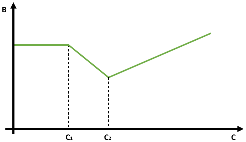
Figure 1 Schematic representation of the organic carbon flux B evolution with carbon content C.

These assumptions about the dependency of the organic matter flux on the surface carbon content C are strong. It is not an easy task to quantify at present the magnitude of carbon burial and oxidation, as some regions are known to be carbon sinks and others are known to be carbon sources. It is an even more complicated task to have an estimation of this budget for different climates and therefore for different carbon contents. However, the results discussed below do not depend on the specific shape chosen for the dependency of the organic matter flux B on the carbon content C. Similar results could be obtained with another dependency, as long as it is non-monotonic with the carbon content C. Here, we have chosen of the simplest cases possible. The shape of the organic matter flux evolution is certainly different and more complex than the one presented here. However, as many processes act on the organic matter flux, some favouring organic matter burial and some favouring organic matter oxidation, we are confident in the fact that the relationship between the organic matter flux B and surface carbon content is non-monotonic.

In our model, carbon and oxygen evolution both depend on the organic matter flux term, which conversely depends on both carbon and oxygen quantities. Therefore, in our model, the carbon and oxygen cycles are coupled via the organic matter flux term. This is the main difference from the model of Paillard (2017), as this results in a non-linear model, where it is possible to have multiple equilibria in the carbon and oxygen system and thus oscillations, even without astronomical forcing.

2.2 Parameter values

We first consider the case where the organic matter flux is not forced astronomically (a_f=0). For simplicity, we have chosen B₀ to be piecewise constant when considering the variations due to carbon. It decreases linearly with oxygen. Therefore, we can write B₀ as follows:

$$\begin{array}{}\text{(7)}& B_{\mathrm{0}}\left(\mathrm{C},\mathrm{O}\right)=B_{\mathrm{0}}\left({\mathrm{C},\mathrm{O}}_{\mathrm{ref}}\right)-\mathit{\delta }\left({\mathrm{O}-\mathrm{O}}_{\mathrm{ref}}\right),\end{array}$$

with

$$\begin{array}{}\text{(8)}& B_{\mathrm{0}}\left({\mathrm{C},\mathrm{O}}_{\mathrm{ref}}\right)=\left\{\begin{array}{ccc}\mathit{\alpha }& \text{for}& \mathrm{C}<{\mathrm{C}}_{\mathrm{1}}\\ \mathit{\alpha }-\mathit{\beta }\left(\mathrm{C}-{\mathrm{C}}_{\mathrm{1}}\right)& \text{for}& {\mathrm{C}}_{\mathrm{1}}<\mathrm{C}<{\mathrm{C}}_{\mathrm{2}}\\ \mathit{\alpha }-\mathit{\beta }\left({\mathrm{C}}_{\mathrm{2}}-{\mathrm{C}}_{\mathrm{1}}\right)+\mathit{\gamma }\left({\mathrm{C}}_{\mathrm{2}}-{\mathrm{C}}_{\mathrm{1}}\right)& \text{for}& \mathrm{C}>{\mathrm{C}}_{\mathrm{2}}\end{array}\right.,\end{array}$$

where δ (δ>0) is the coefficient representing the strength of the organic matter flux evolution with oxygen. The higher δ, the stronger the organic matter flux decrease with oxygen content. α represents the constant value of organic matter flux for low carbon values (C<C₁). −β ($-\mathit{\beta }<\mathrm{0}$) represents the slope of the carbon burial evolution for intermediate carbon values (${\mathrm{C}}_{\mathrm{1}}<\mathrm{C}<{\mathrm{C}}_{\mathrm{2}}$), for which the organic matter flux decreases with increasing carbon content. γ (γ>0) represents the slope of the carbon burial evolution for high carbon values (C>C₂), for which the organic matter flux increases with increasing carbon content. We choose to place ourselves in the case where there are two stable equilibria for the carbon cycle for the current oxygen value (see Sect. 3.1). This corresponds to panel (a) of Fig. 2. These equilibria are called C_eq1ref and C_eq2ref.

Our unforced model therefore contains 13 parameters: the value of carbon emissions associated with volcanism, V₀; the time constant associated with silicate weathering, τ_c; the current oxygen content, O_ref; the two values of the equilibria for O=O_ref, C_eq1ref and C_eq2ref; parameters linked to the shape of the evolution of organic carbon burial with carbon (C₁,C₂, β, γ, α); one parameter linked to the evolution of the organic matter flux with oxygen (δ); and two parameters linked to the evolution of oxidation of elements other than carbon with oxygen (a_ox and b_ox). When the organic carbon burial is forced astronomically, there is one additional parameter, representing the strength of the astronomical forcing: a_f.

O_ref is the current oxygen level and is equal to O${}_{\mathrm{ref}}=\mathrm{1.19}\cdot {\mathrm{10}}^{\mathrm{6}}$ Pg. C_eq1ref and C_eq2ref are the stable equilibria for O=O_ref. We have chosen C_eq1ref to be equal to the pre-industrial carbon content of Earth's surface reservoirs (atmosphere, oceans and biosphere). It is estimated to be around 43 000 PgC (Ciais et al., 2013). We have chosen the second equilibria to be at higher carbon values, C_eq2ref=47 000 PgC. The τ_c constant is set to 200 kyr (Archer et al., 1997). The V₀ value was chosen in order to have δ¹³C values around zero for medium carbon values, $V_{\mathrm{0}}=(\mathrm{5}/\mathrm{8})\cdot (\mathrm{1}/\mathrm{2})({\mathrm{C}}_{\mathrm{eq}\mathrm{1}\mathrm{ref}}+{\mathrm{C}}_{\mathrm{eq}\mathrm{2}\mathrm{ref}})/{\mathit{\tau }}_{\mathrm{c}}=\mathrm{140}$ TgC yr⁻¹. This is a value slightly higher than in Paillard (2017). However, it remains in the range of possible values for carbon emissions from volcanism, estimated to be between 40 and 175 TgC yr⁻¹ (Burton et al., 2013). That C_eq1ref and C_eq2ref are equilibria for O=O_ref in the unforced case gives constraints on the α and γ parameters. Several values of β remain possible with the constraint such that we should have $\mathit{\beta }>\mathrm{1}/\mathrm{2}{\mathit{\tau }}_{\mathrm{c}}$. C₁ and C₂ should be contained between C_eq1ref and C_eq2ref: C${}_{\mathrm{eq}\mathrm{1}\mathrm{ref}}<{\mathrm{C}}_{\mathrm{1}}<{\mathrm{C}}_{\mathrm{2}}<{\mathrm{C}}_{\mathrm{eq}\mathrm{2}\mathrm{ref}}$. In the following, we have taken $\mathit{\beta }=\mathrm{2.4}\cdot \mathrm{1}/\mathrm{2}{\mathit{\tau }}_{\mathrm{c}}$, C${}_{\mathrm{1}}={\mathrm{C}}_{\mathrm{eq}\mathrm{1}\mathrm{ref}}+(\mathrm{1}/\mathrm{3})({\mathrm{C}}_{\mathrm{eq}\mathrm{2}\mathrm{ref}}-{\mathrm{C}}_{\mathrm{eq}\mathrm{1}\mathrm{ref}})=\mathrm{44}\mathrm{333}$ PgC, C${}_{\mathrm{2}}={\mathrm{C}}_{\mathrm{eq}\mathrm{1}\mathrm{ref}}+(\mathrm{2}/\mathrm{3})({\mathrm{C}}_{\mathrm{eq}\mathrm{2}\mathrm{ref}}-{\mathrm{C}}_{\mathrm{eq}\mathrm{1}\mathrm{ref}})=\mathrm{45}\mathrm{667}$ PgC. Changing these parameters would change slightly the form of the unforced oscillations. The δ parameter influences the size of the free oscillations for the oxygen. We have set δ in order to have free oscillations of the size of a few percent of the reference oxygen value. This corresponds to $\mathit{\delta }\sim \mathrm{2}\cdot {\mathrm{10}}^{-\mathrm{7}}$. Different values of the parameters a_ox and b_ox are studied in the following, corresponding to the four possible different cases outlined by the four panels of Fig. 3 (see Sect. 3.1).

3 Results and discussion

Here, we study the results for three different cases to examine the importance of the different processes.

• In a first step, we do not consider astronomical variations of the organic matter flux B. Therefore, organic matter flux only depends on the carbon and oxygen quantities: $B=B_{\mathrm{0}}\left(\mathrm{C},\mathrm{O}\right)$.

• In a second step, we consider a formulation similar to the model of Paillard (2017), where the organic matter flux depends on the astronomical forcing but does not depend on the carbon and oxygen quantities: $B=B_{\mathrm{0}\mathrm{cst}}-a_{\mathrm{f}}F\left(t\right)$, with B_0 cst being a constant.

• In a last step, we consider it to be that the organic matter flux depends on both the astronomical forcing and the carbon and oxygen contents (complete form): $B=B_{\mathrm{0}}\left(\mathrm{C},\mathrm{O}\right)-a_{\mathrm{f}}F\left(t\right)$

3.1 Results without astronomical forcing of the organic matter flux

First, we look at our model results in the case where the organic matter flux is not forced astronomically, corresponding to a_f=0: $B=B_{\mathrm{0}}\left(\mathrm{C}\right(t),\mathrm{O}(t\left)\right)$. This is done in order to better understand the dynamics of the coupled oxygen and carbon system without astronomical forcing. We first consider the system from a theoretical point of view by describing the different possible equilibria. Then, we compute the results numerically for different parameter values.

Equilibria for the carbon are defined as $\frac{\mathrm{d}\mathrm{C}}{\mathrm{d}t}=\mathrm{0}$. From Eq. (2), we get the following:

$$\begin{array}{}\text{(9)}& {\displaystyle \frac{\mathrm{1}}{\mathrm{2}}}{\displaystyle \frac{\mathrm{d}\mathrm{C}}{\mathrm{d}t}}=\left(V-{\displaystyle \frac{W}{\mathrm{2}}}\right)-B.\end{array}$$

Carbon equilibria are thus equivalent to $B=V-W/\mathrm{2}$. As we have assumed $W=\mathrm{C}/{\mathit{\tau }}_{\mathrm{c}}$, and V to be constant, V=V₀, this corresponds to $B=V_{\mathrm{0}}-\mathrm{C}/\left(\mathrm{2}{\mathit{\tau }}_{\mathrm{c}}\right)$. Figure 2 represents schematically the evolution of the organic matter flux term B and the $V-W/\mathrm{2}$ term as a function of the carbon content C. Depending on the relative position of the B curve in relation to the $V-W/\mathrm{2}$ curve, this leads to one or two stable equilibria. For clarity, in the following we will call the B curve (green in the figures) the organic term and the $V-W/\mathrm{2}$ curve (red curve) the inorganic term.

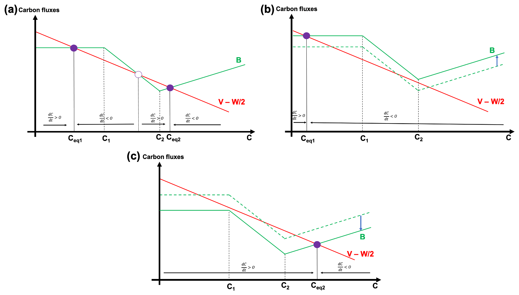
Figure 2 Schematic representation of the organic (green, B) and inorganic (red, $V_{\mathrm{0}}-\mathrm{C}/\left(\mathrm{2}{\mathit{\tau }}_{\mathrm{c}}\right)$) terms as a function of the carbon content C. (a) Case of two equilibria in the carbon system (C_eq1 and C_eq2). (b) Case of one equilibria in the carbon system at a low carbon value (C_eq1). (c) Case of one equilibria in the carbon system at a high carbon value C_eq2.

In the case represented by panel (a) of Fig. 2, the organic and inorganic curves cross at three different locations, meaning that there are three different carbon values C for which an equilibrium is obtained ($\mathrm{d}\mathrm{C}/\mathrm{d}t=\mathrm{0}$). However, only two of these equilibria are stable and are indicated by a full purple circle, while the unstable equilibrium is indicated by an empty purple circle. In the case of the empty circle, if we diverge a little from the equilibria value to higher carbon values, then $V-W/\mathrm{2}>B$ (the red curve is above the green one), and thus $\mathrm{d}\mathrm{C}/\mathrm{d}t>\mathrm{0}$. This small divergence to higher carbon values leads to even higher carbon values: the equilibrium is unstable. The same reasoning can be done if we diverge a little from the equilibrium towards lower carbon values. On the contrary, if we consider the first full purple point from panel (a) of Fig. 2, it is a stable equilibrium. If we diverge a little from this equilibrium towards higher carbon values, then $B>V-W/\mathrm{2}$ (the green curve is above the red), and thus $\mathrm{d}\mathrm{C}/\mathrm{d}t<\mathrm{0}$. The system is brought back towards lower carbon values: the equilibrium is stable. Panel (a) of Fig. 2 represents the case of two stable equilibria in the carbon system. However, it is possible to have only one stable equilibrium in the carbon system if the value of B is higher or lower, as is shown in panels (b) and (c) of Fig. 2. In the case of a higher organic matter flux, there is only one crossing between the green and red curves, as represented in panel (b) of Fig. 2: there is only one equilibrium for the carbon cycle, C_eq1. A similar reasoning to previously shows that this equilibrium is stable. In a similar manner, in the case of a lower organic matter flux, there is only one crossing between the green and red curves, as represented in panel (c) of Fig. 2: there is only one equilibrium for the carbon cycle, C_eq2. This equilibrium is stable. These three configurations of the organic matter flux correspond to different oxygen values. Indeed, as $B\left(\mathrm{C},\mathrm{O}\right)=B\left({\mathrm{C},\mathrm{O}}_{\mathrm{ref}}\right)-\mathit{\delta }(\mathrm{O}-{\mathrm{O}}_{\mathrm{ref}})$, higher oxygen values correspond to a shift of the organic matter (green) curve towards the bottom; the converse is also true. Therefore, it is possible to switch between the configurations if the oxygen evolves.

Similarly to what has been done for the carbon cycle, we look at possible equilibria in the oxygen cycle. In our model, $\mathrm{d}\mathrm{O}/\mathrm{d}t=\mathrm{0}$ corresponds to B= Redox, meaning that the organic matter flux is equal to the oxidation and reduction of elements other than carbon. These terms are represented in Fig. 3. The four different configurations shown in panels (a)–(d) correspond to different values for the slope and intercept of the Redox curve. For these four configurations, the shape of the organic matter flux B (green) curve is similar. For low oxygen values (O<O_lim2), there is only one possible value of the organic matter flux B for each oxygen value. This corresponds to the case displayed in panel (b) of Fig. 2, where there is only one possible equilibrium value for the carbon content C and therefore only one possible value of B for a given oxygen value. For decreasing oxygen values, the organic burial increases. For high oxygen values, (O>O_lim1), there is also only one possible value of the organic matter flux B for each oxygen value. This corresponds to the case displayed in panel (c) of Fig. 2. There is only one possible value for the carbon content C and therefore only one possible value of B for a given oxygen value. These values of organic carbon burial B are lower than the one obtained with O<O_lim2. For intermediate oxygen values (${\mathrm{O}}_{\lim \mathrm{2}}<\mathrm{O}<{\mathrm{O}}_{\lim \mathrm{1}}$), there are two possible equilibrium values for the carbon content C and therefore two possible equilibrium values for the organic matter flux B for a given oxygen value. This corresponds to the case displayed in panel (a) of Fig. 2. The unstable equilibrium is displayed with a dotted line.

Following our hypothesis, the Redox curve is simply a straight line. However, depending on the slope and intercept of the Redox curve, this leads to four different configurations where the (blue) Redox curve either crosses the upper branch of B, the lower branch of B, none of them or both of them. These four different possibilities are schematized in Fig. 3. When the Redox curve crosses the upper branch of B (panel b of Fig. 3), there is one possible equilibrium value for the oxygen ($\mathrm{d}\mathrm{O}/\mathrm{d}t=\mathrm{0}$), represented by the full orange circle. It is a stable equilibrium: if we divert to lower oxygen values, then B>Redox (the green curve is above the blue line), meaning that $\mathrm{d}\mathrm{O}/\mathrm{d}t>\mathrm{0}$, and the oxygen value increases back towards equilibrium. Similarly, when the Redox curve crosses the lower branch of B (panel c of Fig. 3), there is one possible equilibrium value for the oxygen. This is also a stable equilibrium. When the Redox curve crosses both the upper and lower branches of B (panel d of Fig. 3), it also crosses the middle, unstable branch. There are three possible equilibrium values for the oxygen, two of which are stable (the crossing with the upper and lower branch). For these three cases (panels b, c and d of Fig. 3), the system will converge towards an equilibrium value (C_eq, O_eq) and remain in this state, as these are stable equilibria. When the equilibrium is reached, the carbon and oxygen content will not evolve anymore. The organic matter flux and the δ¹³C will therefore also not change.

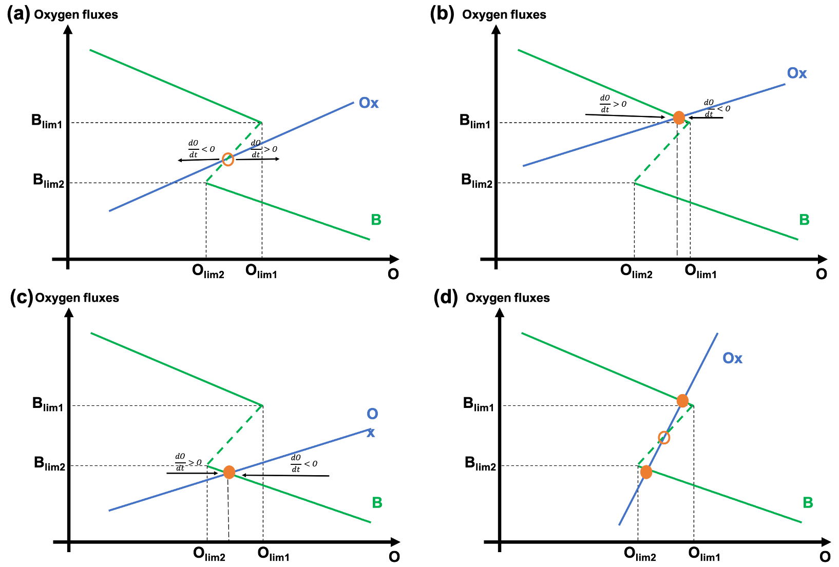
Figure 3 Schematic representation of the organic term (B, green curve) and the Redox term (blue curve) as a function of the oxygen content O. Four different cases are displayed, depending on the slope and intercept of the Redox curve: (a) one unstable equilibrium, (b) and (c) a stable equilibria, and (d) two stable equilibria

However, the situation is different in the case where the Redox curve does not cross the lower or upper branch of B but crosses the middle branch (dashed line), as represented in panel (a) of Fig. 3. This branch is not stable from the perspective of carbon (it corresponds to the unstable equilibria of Fig. 2). It is also not a stable equilibrium for oxygen. In this case, no equilibrium is reached for the (C, O) system, and oscillations of the oxygen and carbon content can be obtained without astronomical forcing of the organic matter flux. The organic matter flux and the δ¹³C therefore also oscillate.

To illustrate these cases, we run our model without astronomical forcing. For conciseness reasons, we consider only two out of the four possible cases described above. We will consider the two cases for which the Redox curve crosses the unstable middle branch, corresponding to panels (a) and (d) of Fig. 3. We define the parameter a_lim as $a_{\lim }=(B_{\lim \mathrm{1}}-B_{\lim \mathrm{2}})/({\mathrm{O}}_{\lim \mathrm{1}}-{\mathrm{O}}_{\lim \mathrm{2}})$. If a_ox>a_lim, this corresponds to the case of panel (d) of Fig. 3. If a_ox<a_lim, this corresponds to the case depicted in panel (a) of Fig. 3.

3.1.1  a_ox>a_lim

The model is run for 100 Myr with $a_{\mathrm{ox}}=\mathrm{1.5}\cdot a_{\lim }$ for one specific set of model parameters. The simulations start from different initial values for the carbon and oxygen. The Redox curve intercept parameter, b_ox, is chosen in order to follow the configuration of panel (d) of Fig. 3, where the Redox curve crosses the B curve three times. The carbon, oxygen, organic matter flux and δ¹³C evolution over time are displayed in Fig. 4.

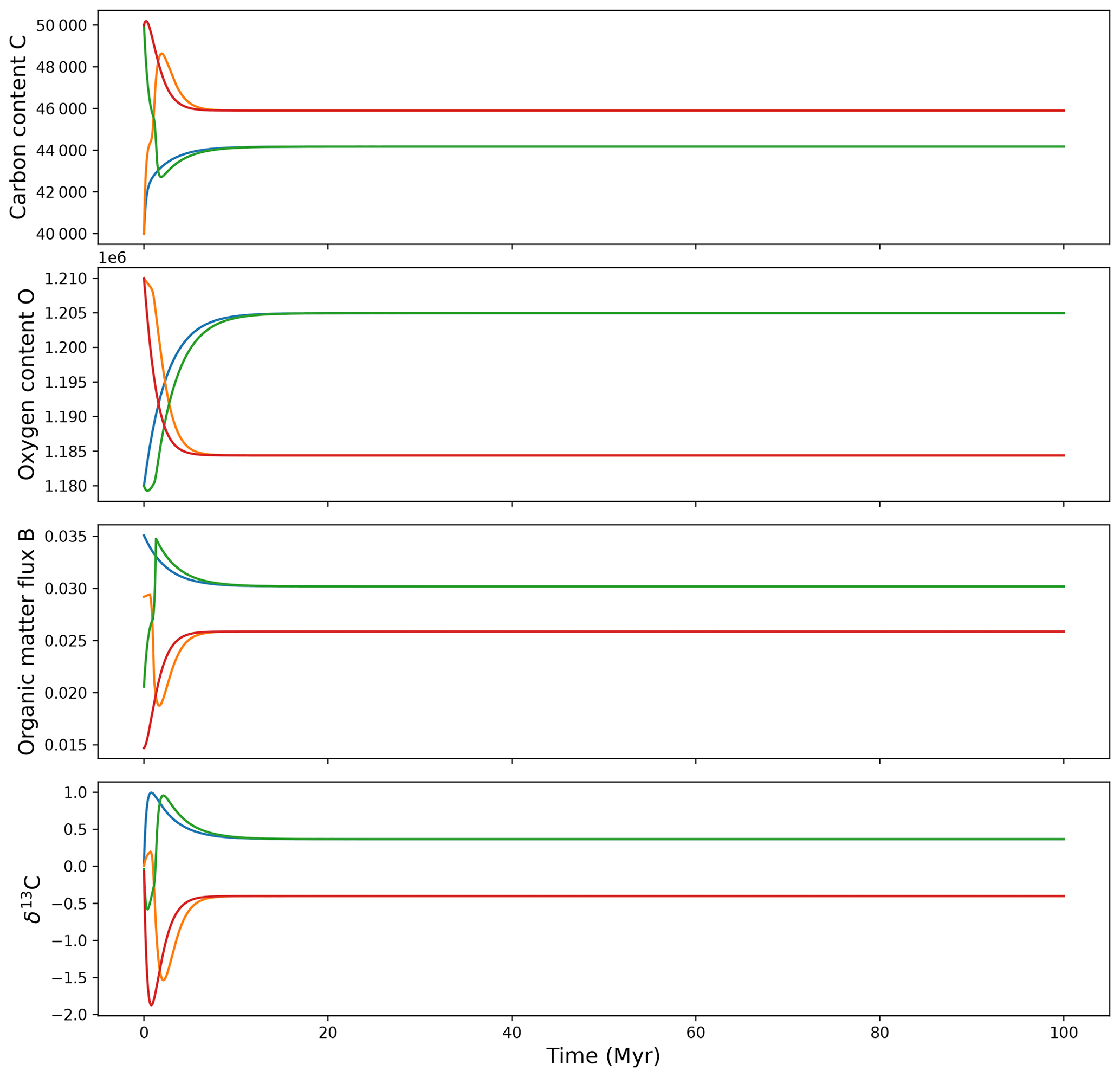
Figure 4 Modelled carbon content, C; oxygen content, O; organic matter flux, B; and δ¹³C evolution in the case without astronomical forcing for different initial states. Case a>a_lim.

An equilibrium is reached in less than 10 Myr for all the simulations. The equilibrium value depends on the initial conditions. This is expected, as there are two stable equilibria for the (C, O) system in this configuration. In the case of a different value of the parameter b_ox, leading to a single crossing with the B curve (case of panels b and c of Fig. 3), an equilibrium would also be reached. The only difference is that the equilibrium would not depend on initial conditions, as there is only one possible equilibrium value.

3.1.2  a_ox<a_lim

The model is run for 100 Myr with $a_{\mathrm{ox}}=\mathrm{0.5}\cdot a_{\lim }$ for one specific set of model parameters, starting from different initial values for the carbon and oxygen. The parameter b_ox is chosen in order to follow the configuration of panel (a) of Fig. 3, where the Redox curve only crosses the unstable part of the B curve. The carbon, oxygen, organic matter flux and δ¹³C evolution over time are displayed in Fig. 5.

In this case, no equilibrium is reached, and the system oscillates. The amplitude of the oscillations for the carbon is around 6000 PgC. The δ¹³C oscillations have an amplitude around 2.5 ‰. The frequency of the oscillations is identical for the different initial conditions, and only the phase is different. The oscillations have a period of approximately 15 Myr with the parameter set used in this example. The frequency and shape of the oscillations depend on the model parameters. For example, for higher values of the δ parameter, the system would oscillate more quickly.

To sum up, we have detailed here a simple case without astronomical forcing of the organic matter flux B. In this case, there are two possibilities for the evolution of the (C, O) system. If there is at least one stable equilibrium for the oxygen (case of panels b, c and d of Fig. 3), then the system will converge towards an equilibrium (C_eq, O_eq), and the modelled δ¹³C will also converge towards an equilibrium. If there is no stable equilibrium for the oxygen (case of panel a of Fig. 3), the (C, O) system will oscillate freely, and the modelled δ¹³C will also oscillate. However, in our model, the organic matter flux is also forced astronomically through a dependency on eccentricity. This makes the situation more complex. When a stable equilibrium is reached in a case without astronomical forcing, the equilibrium can become unstable in the forced case if the astronomical forcing is relatively strong (relatively high values of the a_f parameter). In this case, the astronomical forcing pushes the system away from its equilibrium towards another. This will be detailed in the third result section.

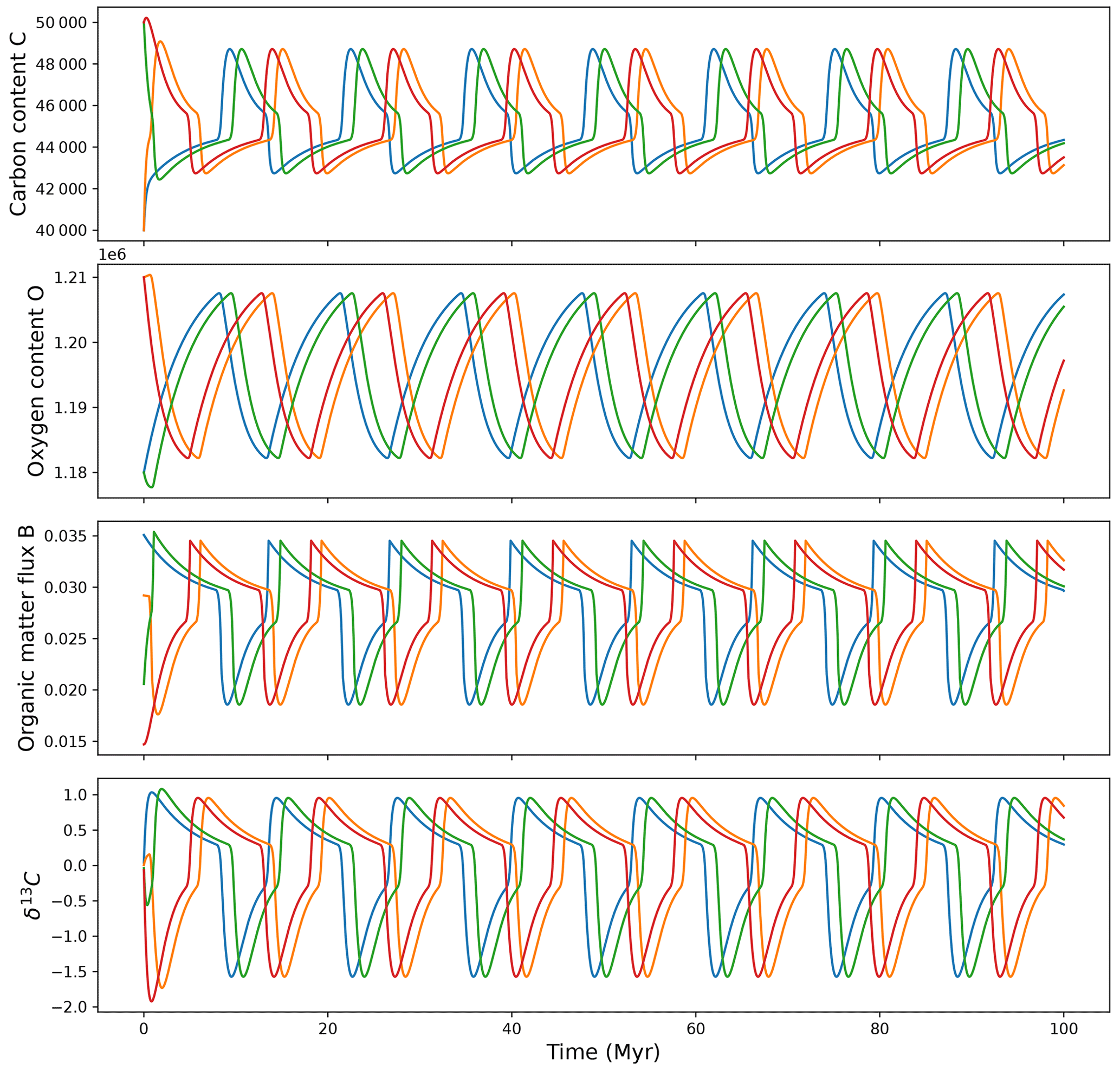
Figure 5 Modelled carbon content, C; oxygen content, O; organic matter flux, B; and δ¹³C evolution in the case without astronomical forcing for different initial states. Case a<a_lim.

3.2 Results without oscillatory dynamics – organic matter flux not depending on surface oxygen.

In a second step, we study our model results in the case where the organic matter flux does not depend on surface carbon and oxygen quantities but is solely forced by the astronomical forcing: $B=B_{\mathrm{0}\mathrm{cst}}-a_{\mathrm{f}}F\left(t\right)$, where B_0 cst is a constant. This is close to the model of Paillard (2017). In this case, we have no coupling anymore between the carbon and the oxygen cycle, and the system is linear, with an astronomical forcing.

$$\begin{array}{}\text{(10)}& \left\{\begin{array}{c}\frac{\mathrm{d}\mathrm{C}}{\mathrm{d}t}=-\frac{\mathrm{1}}{{\mathit{\tau }}_{\mathrm{c}}}\mathrm{C}+c_{\mathrm{1}}-\mathrm{2}{a}_{\mathrm{f}}F\left(t\right)\\ \frac{\mathrm{d}\mathrm{O}}{\mathrm{d}t}=-a_{\mathrm{ox}}\mathrm{O}+c_{\mathrm{2}}+a_{\mathrm{f}}F\left(t\right),\end{array}\right.\end{array}$$

with c₁ and c₂ being constants: $c_{\mathrm{1}}=\mathrm{2}(V_{\mathrm{0}}-B_{\mathrm{0}})$, $c_{\mathrm{2}}=B_{\mathrm{0}}-b$. As a_ox>0 and $\frac{\mathrm{1}}{{\mathit{\tau }}_{\mathrm{c}}}>\mathrm{0}$, the system is stable. Without the astronomical forcing, it would converge towards an equilibrium. The addition of the astronomical forcing yields oscillations around it.

In the following, we have run the model with the same parameters as previously for different values of the a_f parameter. In Fig. 6, the evolutions of carbon, oxygen, organic carbon flux and δ¹³C over time are displayed for a_f=0.01 (green curves), a_f=0.03 (orange curves) and a_f=0.05 (blue curves). There are oscillations around an equilibrium value for the carbon and the δ¹³C. Changing the a_f value changes neither the shape nor the frequency of the oscillations. It only changes their amplitude. For the δ¹³C, the oscillation amplitude varies from around 0.5 ‰ for the weakest astronomical forcing considered (a_f=0.01) to 2 ‰ for the strongest astronomical forcing considered (a_f=0.05). For the carbon, the oscillation amplitude varies from around 1000 to 6000 PgC.

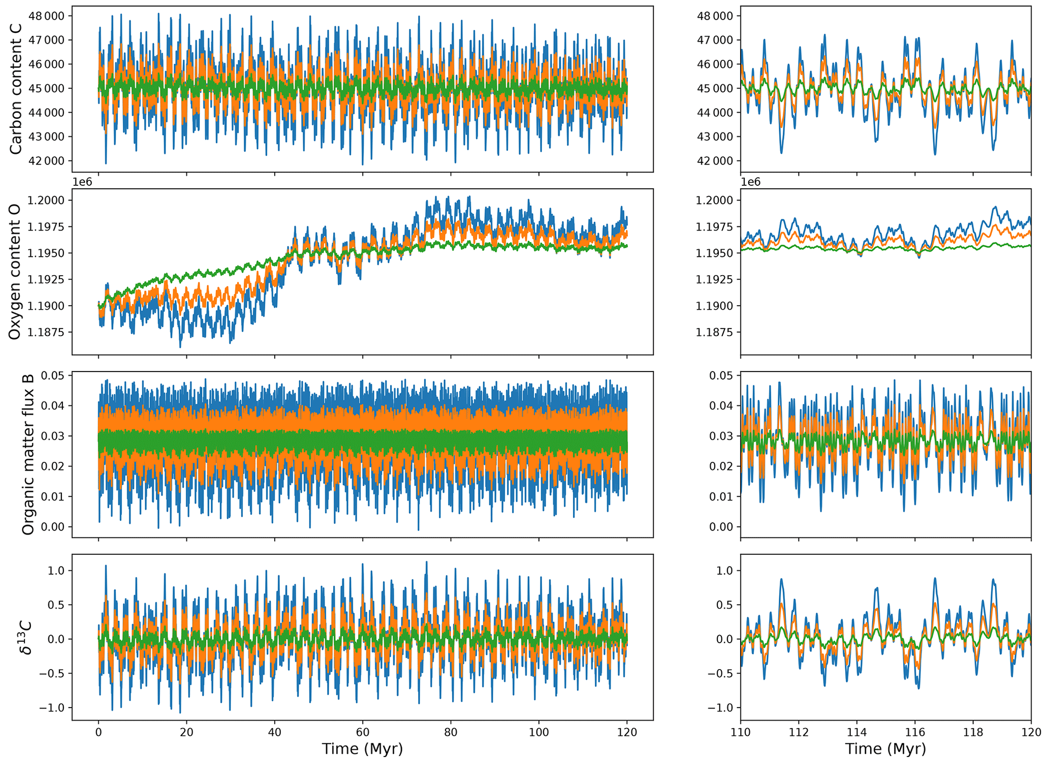
Figure 6 Modelled carbon content, C; oxygen content, O; organic matter flux, B; and δ¹³C for different a_f values (a_f=0.01 in green, a_f=0.03 in orange, and a_f=0.05 in blue) when B₀ is a constant. The right panel is a zoom on the last 10 Myr of the simulation.

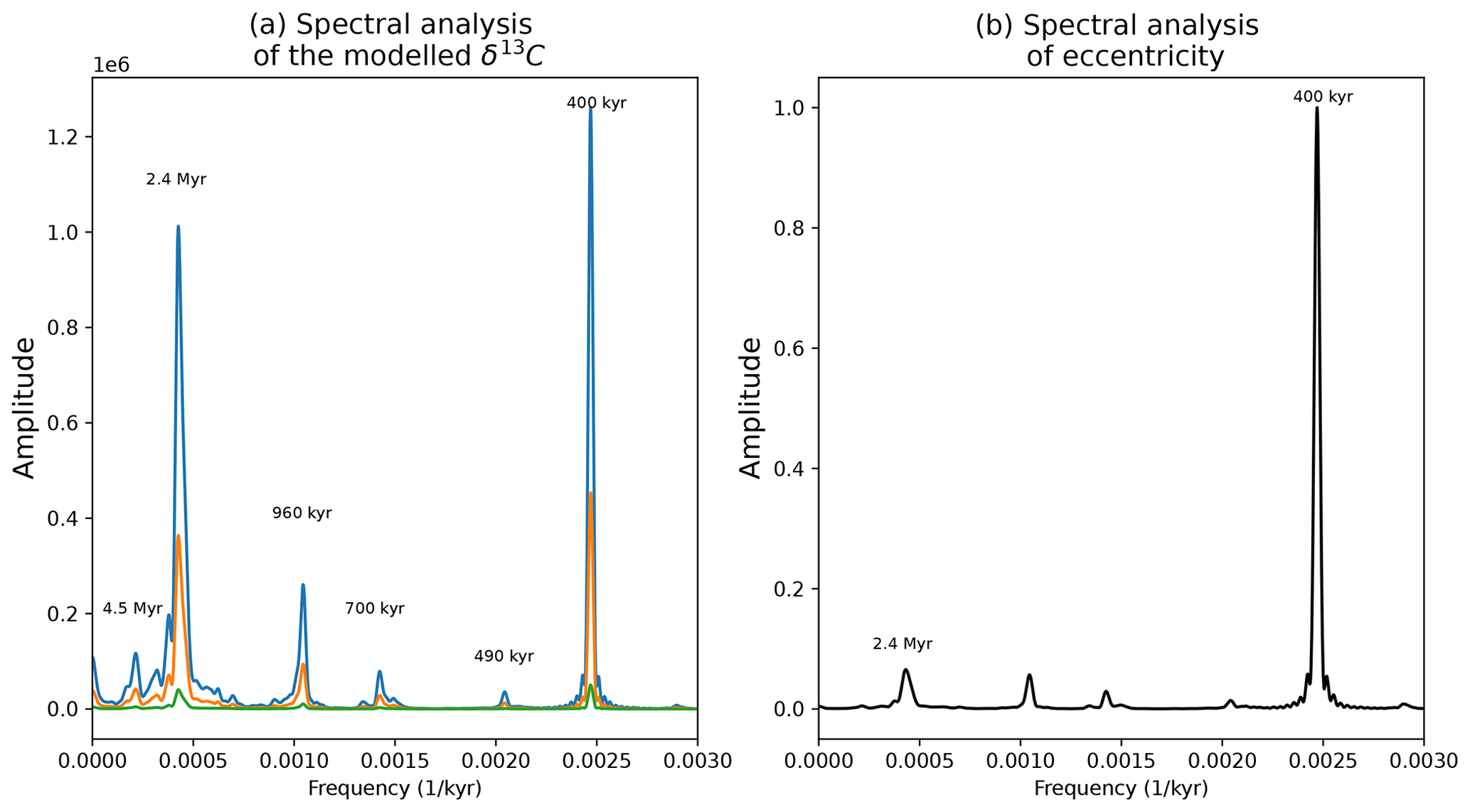
Figure 7 (a) Normalized spectral analysis of the resulting δ¹³C for different a_f values (a_f=0.01, 0.03 and 0.05 in green, orange and blue) when B₀ is a constant. (b) Spectral analysis of the eccentricity input forcing.

The spectral analysis of the δ¹³C curve is shown in panel (a) of Fig. 7. The dominant frequencies of the δ¹³C oscillations are 400 kyr and 2.4 Myr. These frequencies are present in the input forcing (the eccentricity). The 400 kyr frequency is already strong in the input forcing. However, the 2.4 Myr frequency is of low power in the eccentricity spectra but is strong in the modelled δ¹³C. The δ¹³C spectral analysis also contains a weaker ∼ 4.5 Myr peak. This frequency is of very low amplitude in the input eccentricity forcing. As in the Paillard (2017) model, we are able to produce 400 kyr and 2.4 Myr cycles in δ¹³C through the astronomical forcing of organic matter flux. However, as this model is linear, it is not possible to produce longer-term cycles with a high amplitude corresponding to frequencies with very low amplitude in the eccentricity spectra. A non-linear model is needed to produce larger periods with a strong amplitude in δ¹³C with a simple eccentricity forcing. This is the case with our model when we add the dependency of the organic matter flux on the carbon and oxygen contents. The results for specific parameter values are discussed in the next section.

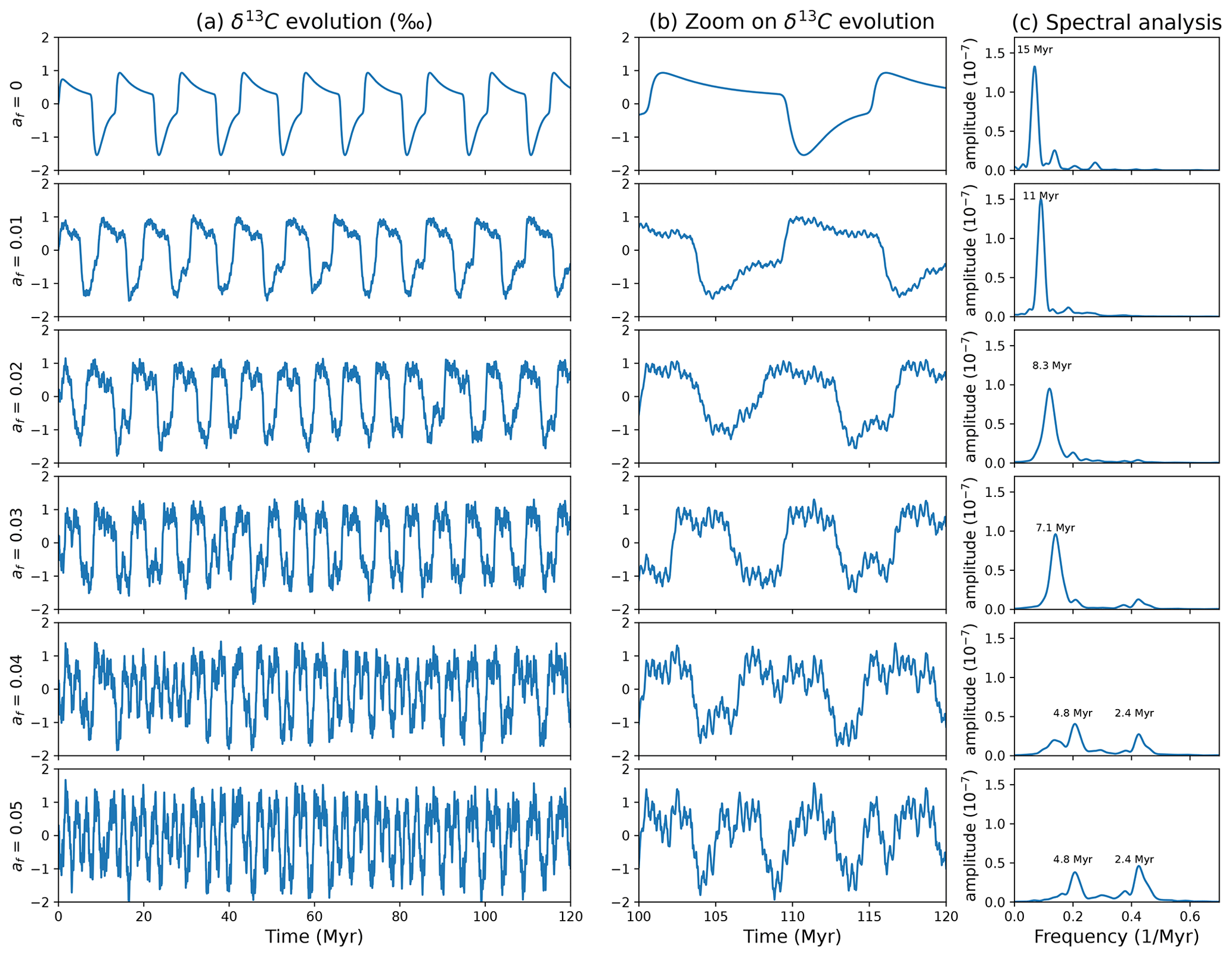
Figure 8 Case A. (a) Modelled δ¹³C for different a_f values, and $a=\mathrm{0.5}\cdot a_{\lim }$. (b) Zoom on the last 20 Myr of the simulation. (c) Spectral analysis of the modelled δ¹³C.

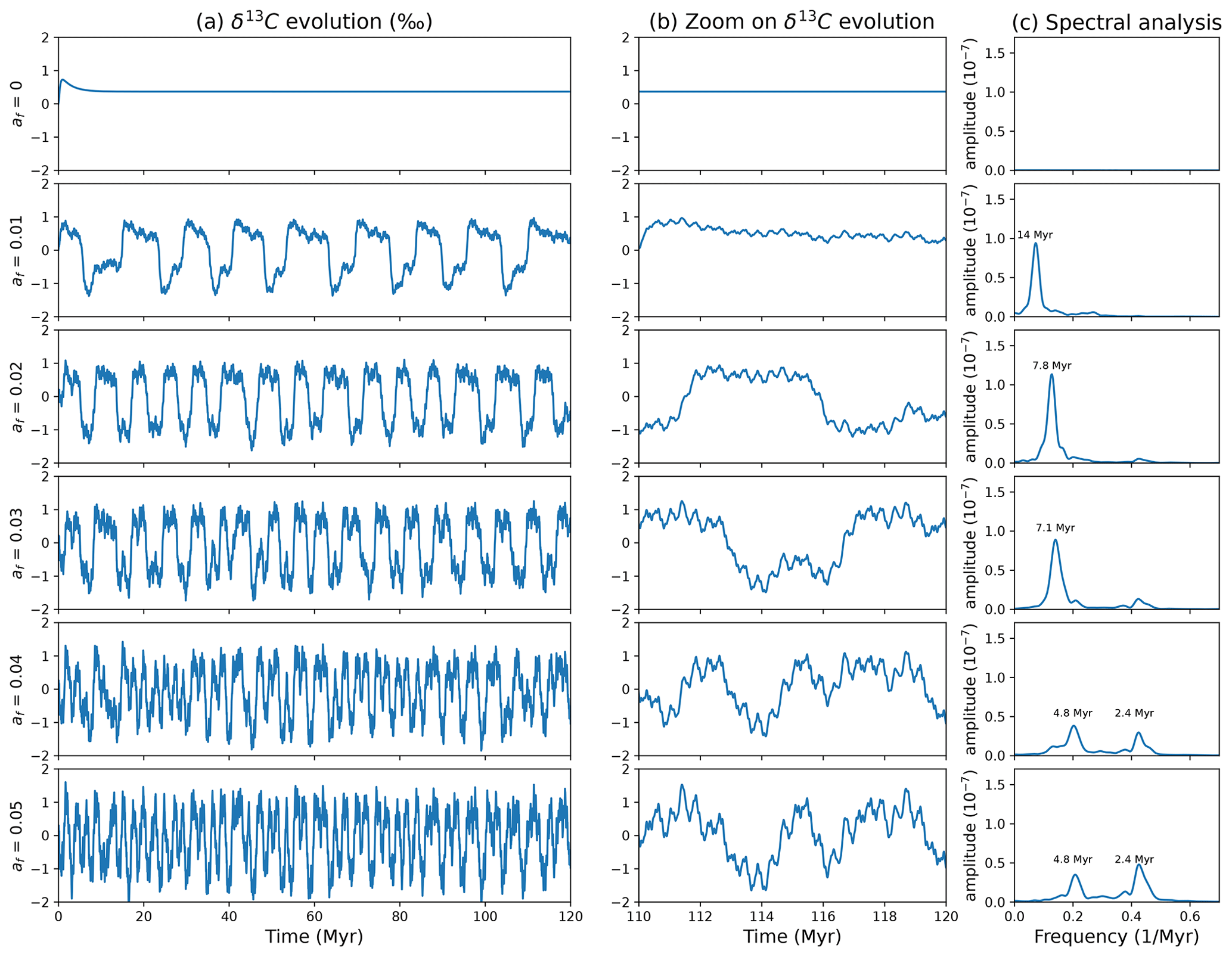
Figure 9 Case B. (a) Modelled δ¹³C for different a_f values, and $a=\mathrm{1.5}\cdot a_{\lim }$. (b) Zoom on the last 20 Myr of the simulation. (c) Spectral analysis of the modelled δ¹³C.

3.3 Complete model: astronomical forcing of the organic matter flux and dependency on carbon and oxygen quantities

Here, we use the complete form of the organic matter flux, as described in Sect. 2.1. The organic matter flux, B, depends on the surface carbon quantity, C; the surface oxygen quantity, O; and the astronomical forcing, F(t): $B=B_{\mathrm{0}}\left(\mathrm{C}\right(t),\mathrm{O}(t\left)\right)-a_{\mathrm{f}}F\left(t\right)$. We perform simulations for different a_f parameter values ranging from a_f=0 to a_f=0.05. This corresponds to the different relative importance of the astronomical forcing on the organic matter flux. The simulations are run over 120 Myr. We perform these simulations in two different cases. The first (case A) corresponds to a situation where the system oscillates freely for a_f=0. This corresponds to panel (a) of Fig. 3. The second one (case B) corresponds to a situation where the system does not oscillate for a_f=0 (presence of a stable equilibria). In our case, we have taken a situation corresponding to panel (b) of Fig. 3. The evolution of δ¹³C in both these cases is displayed in panels (a) of Figs. 8 and 9. A zoom on the last 20 Myr of the simulation is provided in panels (b). The spectral analysis of the modelled δ¹³C is displayed in panels (c). The spectral analyses were carried out with the Blackman–Tuckey method implemented in the AnalySeries software (Paillard et al., 1996).

In case A, the δ¹³C oscillates freely when the system is not forced astronomically (a_f=0), with an amplitude around 2 ‰. For a relatively small influence of the astronomical forcing (a_f=0.01), the shape of the large, free oscillations is still visible, and small oscillations of amplitude around 0.1 ‰ occur around it. However, the frequency of the free oscillations is affected by the astronomical forcing and differs from the unforced case. In case B, there are no oscillations for a_f=0. For a_f>0, oscillations similar to case A occur. In both cases, for higher values of a_f, the signal is dominated by oscillations of a lower period. The dominant, low-period oscillations have an amplitude of around 2 ‰, and the smaller higher-frequency oscillations have an amplitude of around 0.05 ‰. Oscillations of 400 kyr are present for all cases where the system is forced astronomically. However, their relatively low amplitude makes them hard to notice in the spectral analysis, especially for low a_f values. As the relative strength of the astronomical forcing increases (a_f increases), the power of the 400 kyr oscillations becomes stronger. The dominant period of the oscillations decreases with increasing a_f parameter.

In both cases, the addition of the astronomical forcing changes the behaviour of the coupled system, and we are able to obtain oscillations on the δ¹³C of several million years. In case A, the output signal has a dominant frequency that differs from the frequency of self-sustained oscillations of the unforced system. In case B, it is worth emphasizing that, even if there are no self-sustained oscillations without astronomical forcing, the addition of the astronomical forcing of the organic matter flux also leads to multi-million-year cycles in δ¹³C.

One important feature to notice is that, when the a_f parameter decreases, the output signal dominant period does not decrease continuously. Figure 10 represents the dominant period of the signal depending on the a_f parameter for different parameter sets. The plot shows “steps”: there are preferential periods, meaning that, for a range of a_f values, the output dominant period remains the same. The 2.4 Myr periodicity and its multiples are schematized with dotted blue lines.

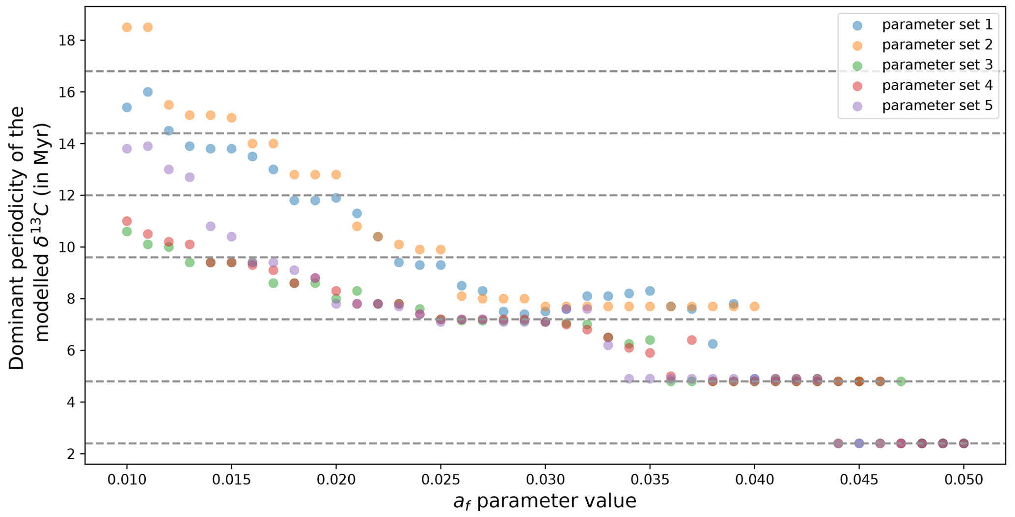
Figure 10 Dominant period of the modelled δ¹³C as a function of the a_f value for different parameter sets.

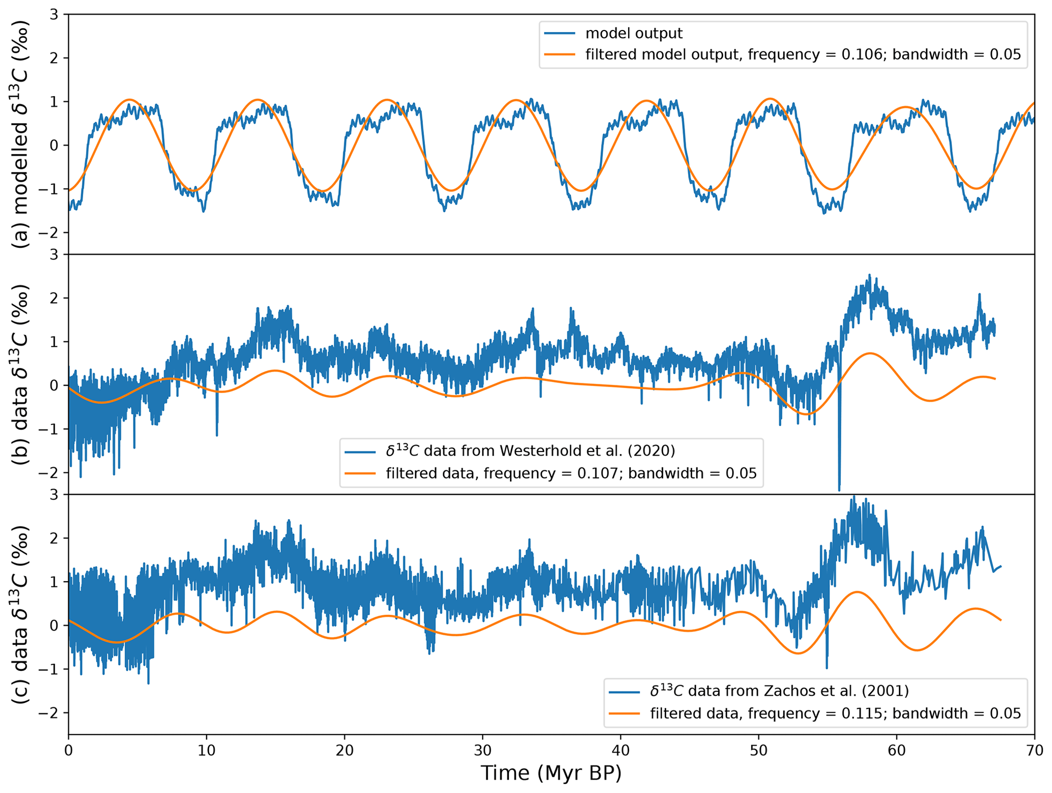
Figure 11 Comparison of (a) the modelled δ¹³C and (b) deep-sea record δ¹³C (data are from Westerhold, 2020) in blue and filtered (frequency = 0.107; bandwidth = 0.05) in orange. The modelled δ¹³C shown was taken among the model outputs that produce ∼ 9 Myr cyclicities.

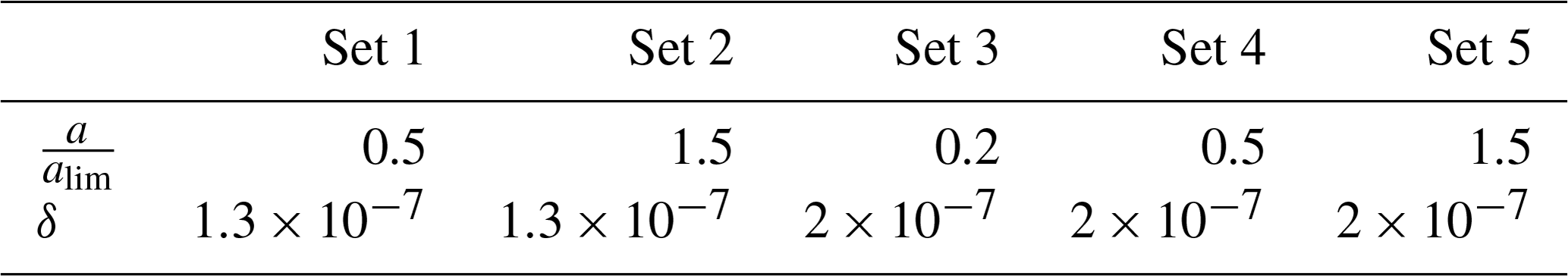
Table 1 Value of the different parameter sets displayed in Fig. 10.

For large a_f values (around 0.4–0.5), the dominant frequency is 2.4 Myr. Both 2.4 and 4.8 Myr periodicities are present in the spectral analysis. As the a_f parameter decreases slightly, the 4.8 Myr periodicity becomes dominant. It is particularly striking that, for each parameter set, it is not possible to have a dominant frequency value between 2.4 and 4.8 Myr. The 4.8 Myr periodicity is the double of the 2.4 Myr periodicity of eccentricity. As the a_f parameter decreases, a period around 7 Myr becomes dominant. It is between 7.2 and 7.7, depending on the parameter set. This periodicity is not present in the eccentricity spectra. However, it corresponds to the triple of the 2.4 Myr periodicity. It is possible to obtain dominant frequencies between 4.8 and 7 Myr. However, this is limited to very specific cases (specific a_f values for specific parameter values). On the contrary, the ∼ 7 Myr period is dominant for a wide range of a_f parameters for all parameter sets (between a_f=0.025 and a_f=0.04 depending on the parameter set). Decreasing again the a_f parameter produces longer periods. The isolation of a preferential periodicity is not as clear as for the 2.4, 4.8 and ∼ 7 Myr frequencies, and the rise of the dominant frequency of the output signal with the a_f parameter decrease becomes more continuous. However, for each parameter set, there is a small step around the fourth multiple of 2.4 Myr, ∼9.6 Myr (between 9 and 10 Myr, depending on the parameter set). The corresponding a_f interval is much smaller than in the case of the 4.8 and ∼ 7 Myr periods. As the a_f parameter decreases again, the evolution of the dominant frequencies seems to vary in a non-continuous way with preferred frequencies, but the behaviour is less clear. The presence of preferred periods suggests a mechanism of phase locking, which allows the multiples of the 2.4 Myr eccentricity period to be obtained.

As a response to a simple eccentricity forcing, our non-linear model is able to produce multi-million-year cycles of periods absent from the input forcing (or present with very low amplitude), most probably via a mechanism of phase locking.

However, the shape of the oscillations obtained is quite far away from the data. For each parameter set, there are values of the a_f parameter that produce ∼ 9 Myr cycles in the δ¹³C. One of them is displayed in Fig. 11. For comparison, δ¹³C from deep-sea records (Zachos et al., 2001; Westerhold, 2020) are also shown. In the modelled δ¹³C, there are oscillations between high and low δ¹³C values, and the shift between the low and high values is quite sudden. This is due to the fact that, in our model, the δ¹³C has two equilibrium values when the organic matter flux is not forced astronomically. When the astronomical forcing is added, oscillations occur around one equilibrium value until the astronomical forcing becomes strong enough to push the system towards the second equilibrium; 400 kyr cycles are also noticeable on top of the multi-million-year oscillations. However, their strength is underestimated compared to the data.

At these timescale, many other processes are not taken into account here, such as plate tectonics (Müller and Dutkiewicz, 2018); likewise, other geochemical cycles could play a role and influence the carbon cycle. Our model is simple and excludes many processes that could be of importance, and other mechanisms can be considered to produce internal oscillatory dynamics. For instance, we have assumed a constant Ca²⁺ concentration in the ocean. This is a limitation of our model. In particular, including calcium variations could change and complexify the relationship between global carbon content C and atmospheric CO₂. In this model, we have linked the carbon and oxygen cycles through the organic matter flux term. The “real” dependency of the organic carbon flux B on the surface carbon C and thus on climate is probably much more complicated than the shape envisaged here. However, the results obtained are generic, and multiple equilibria and self-sustained oscillations (without any external forcing like eccentricity) could be obtained in an Earth system with a different shape of B corresponding to different mechanisms. One of the conditions to allow for multiple equilibria to exist is to have a non-monotonic dependency of B(C). That B(C) has the same shape as the one assumed in this study is highly unlikely, but the fact that B varies in a non-monotonic way with climate and thus with the carbon content C is highly probable due to the variety of processes involved that might be favoured for certain climates and thus for lower or higher carbon values. One could also imagine the obtainment of more complex oscillations involving the sulfur cycle. Oxidation of sulfide minerals produces sulfuric acid, which can react with carbonate minerals and thus release CO₂ (Torres et al., 2014). Sulfide oxidation also affects the oxygen content. Here, we have based the oscillations on the (C, O) elements, but other mechanisms could certainly be considered.

4 Conclusions

Multi-million-year oscillations are present in the δ¹³C records throughout the Cenozoic and part of the Mesozoic. It has been suggested that these variations could be related to astronomical forcing of organic matter fluxes. However, no modelling study has been able to perform such long oscillations through astronomical forcing of organic matter fluxes. Here, we have proposed a mathematical mechanism, compatible with biogeochemistry, that could explain the presence of multi-million-year cycles in the δ¹³C record and their stability over time as a result of preferential phase locking to multiples of the 2.4 Myr eccentricity period. A simple, linear astronomical forcing alone cannot produce multi-million-year cycles longer than 2.4 Myr with a strong amplitude, but the presence of multiple equilibria in our model allows for the extraction of longer periods. Our results show that astronomical forcing, superimposed to internal oscillations of the climate system (like here, with carbon and oxygen), is a way to obtain very-long-term cycles of δ¹³C with periodicities that are not directly present in the initial astronomical forcing.