the Creative Commons Attribution 4.0 License.
the Creative Commons Attribution 4.0 License.
 | 19 Oct 2022
Constraining low-frequency variability in climate projections to predict climate on decadal to multi-decadal timescales – a poor man's initialized prediction system
Markus G. Donat
Pablo Ortega
Francisco J. Doblas-Reyes
Carlos Delgado-Torres
Margarida Samsó
Pierre-Antoine Bretonnière
Near-term projections of climate change are subject to substantial uncertainty from internal climate variability. Here we present an approach to reduce this uncertainty by sub-selecting those ensemble members that more closely resemble observed patterns of ocean temperature variability immediately prior to a certain start date. This constraint aligns the observed and simulated variability phases and is conceptually similar to initialization in seasonal to decadal climate predictions. We apply this variability constraint to large multi-model projection ensembles from the Coupled Model Intercomparison Project phase 6 (CMIP6), consisting of more than 200 ensemble members, and evaluate the skill of the constrained ensemble in predicting the observed near-surface temperature, sea-level pressure, and precipitation on decadal to multi-decadal timescales.
We find that the constrained projections show significant skill in predicting the climate of the following 10 to 20 years, and added value over the ensemble of unconstrained projections. For the first decade after applying the constraint, the global patterns of skill are very similar and can even outperform those of the multi-model ensemble mean of initialized decadal hindcasts from the CMIP6 Decadal Climate Prediction Project (DCPP). In particular for temperature, larger areas show added skill in the constrained projections compared to DCPP, mainly in the Pacific and some neighboring land regions. Temperature and sea-level pressure in several regions are predictable multiple decades ahead, and show significant added value over the unconstrained projections for forecasting the first 2 decades and the 20-year averages. We further demonstrate the suitability of regional constraints to attribute predictability to certain ocean regions. On the example of global average temperature changes, we confirm the role of Pacific variability in modulating the reduced rate of global warming in the early 2000s, and demonstrate the predictability of reduced global warming rates over the following 15 years based on the climate conditions leading up to 1998. Our results illustrate that constraining internal variability can significantly improve the accuracy of near-term climate change estimates for the next few decades.
- Article
(10284 KB) - Full-text XML
-
Supplement
(4191 KB) - BibTeX
- EndNote


In the context of ongoing climate change, predicting the climate evolution over the coming decades is important to enable targeted adaptation to the anticipated changes. While increasing greenhouse gas concentrations cause a general global warming (IPCC, 2021), different modes of climate variability can regionally amplify or counteract the warming-related effects.
To obtain information about the expected climate in the future, climate projections simulate the responses of the Earth system to specified radiative forcing scenarios (Eyring et al., 2016; Taylor et al., 2012). These climate projections are affected by different uncertainties related to the forcing scenario chosen, the climate model used, and the phasing of internal variability. For projections of near-term climate change in the next 20 to 30 years, internal variability is the dominating source of uncertainty at regional scales (Hawkins and Sutton, 2009, 2011; Lehner et al., 2020), while at longer timescales the scenario choice becomes increasingly important.
Decadal predictions, initialized towards observational states, are designed to exploit the predictability arising from both internal climate variability (Meehl et al., 2021; Kushnir et al., 2019), which is achieved by aligning the phases of the variability modes in the model simulations with our best estimate of the real-world state, and from externally forced changes (Doblas-Reyes et al., 2013). These initialized decadal predictions show significant improvements in terms of added skill as compared to the uninitialized projections (e.g., Smith et al., 2019, 2020). However, the decadal predictions often suffer from initialization shocks and the subsequent drift towards the model's preferred climate state which can significantly reduce the overall skill of a decadal prediction system (e.g., Bilbao et al., 2021). In addition, the decadal hindcasts involve running very large ensembles of simulations and are therefore computationally expensive, which has traditionally limited their production to the next 10 years with relatively small ensemble sizes (Boer et al., 2016).
As an alternative, constraining decadal variability in large ensembles of future projection simulations can improve climate information and reduce uncertainty of projections for the next few decades. Different approaches have been explored to constrain internal variability in climate projections (e.g., Hegerl et al., 2021). An important advantage of these approaches, based on sub-selecting members of a set of transient climate simulations, is that predictions made based on these simulations are consistent with the model-specific climate attractor, and not affected by shock, drift, or related artifacts (Hazeleger et al., 2013; Smith et al., 2013; Bilbao et al., 2021). On seasonal to interannual timescales, Ding et al. (2018) made skillful predictions of tropical Pacific sea surface temperatures (SSTs) by finding model analogues similar to the observed state and using the subsequent trajectories of those analogues as forecasts. Similarly, Menary et al. (2021) developed an analogue approach to predict decadal-scale variations in the North Atlantic region.
On decadal to multi-decadal timescales, Befort et al. (2020) and Mahmood et al. (2021) have recently proposed approaches to constrain projections based on their agreement with decadal predictions and demonstrated some added value beyond the time period covered by decadal predictions. However, the aforementioned limitations affecting the initialized decadal predictions can also limit the added value of the constrained ensembles. Here we implement an approach similar to Mahmood et al. (2021), however using climate observations for the constraining criteria instead of decadal prediction data. In particular, we use multi-annual averages of sea surface temperature (SST) anomaly patterns as constraining criterion. In essence, this method exploits ensembles of already available model simulations to sub-select those members in closest agreement with the contemporary and/or immediately preceding observed SST anomaly patterns. Such member selection method thus works as a poor man's initialization to predict climate in the following decades.
In the following we describe the data and approach used to implement the poor man's initialized prediction system (Sect. 2). We then demonstrate its application and evaluate the skill in predicting temperature, sea level pressure, and precipitation globally, in comparison to state-of-the-art initialized predictions contributing to the Decadal Climate Prediction Project (DCPP; Boer et al., 2016), and discuss the sensitivity to some of the various choices to be made during the selection procedure. We further outline the applicability of this approach to attribute predictability of specific decadal-scale phenomena to certain ocean regions (Sect. 3). We conclude this paper with a summary and discussion of this poor man's initialized prediction approach in the context of other existing prediction systems (Sect. 4).
We use climate model simulation data from the Coupled Model Intercomparison Project phase 6 (CMIP6) simulations (Eyring et al., 2016). A total of 212 ensemble members from 32 different models were available, composed of transient historical simulations (hereafter referred to as “unconstrained”, see Table S1 in the Supplement) until 2014 and continued with future projection simulations following the shared socioeconomic pathway (SSP2-45) forcing scenario (from 2015 onwards). We also use 93 members from 9 different models of the CMIP6/DCPP-A initialized decadal hindcasts in order to evaluate the skill of the constrained projections in comparison to actual initialized predictions.
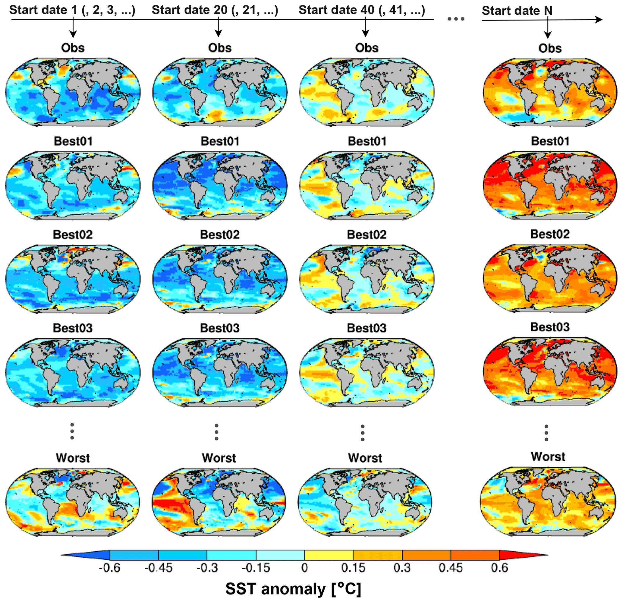
Figure 1A schematic illustration of the constraining methodology in which observed SST anomaly patterns (as in the top row) are used to compute spatial pattern correlations with individual historical ensemble members. Based on these pattern correlations, the historical ensemble members are ranked from the one with the best agreement with the observed state (e.g., Best01, Best02, Best03) to the worst agreement. For conciseness, we only show here the observed and the ranked historical member anomaly patterns of four start dates, however this ranking procedure is repeated every year using 9-year average SST anomalies prior to starting a prediction. For each start date, we select the 30 top ranking members to make predictions on decadal to multi-decadal timescales.
The observational data set used in this study to constrain the climate projections is the Extended Reconstructed Sea Surface Temperature version 5 dataset (ERSSTv5; Huang et al., 2017) from the National Oceanic and Atmospheric Administration (NOAA). Surface temperature from HadCRUT4.6 (Morice et al., 2012), sea level pressure (SLP) from Japanese 55-year Reanalysis (JRA-55; Kobayashi et al., 2015), and precipitation from Global Precipitation Climatology Center (Schamm et al., 2014) were used to evaluate the hindcasts on decadal and multi-decadal timescales. All data sets used in this study were converted to monthly mean anomalies relative to the reference climatological period of 1981-2010. We also evaluated the skill of the hindcasts using a different set of observational data for surface temperature, SLP, and precipitation (see Sect. S1 in the Supplement), to confirm the robustness of the results for different reference datasets.
The constraining procedure involves comparing SST anomaly patterns of individual unconstrained members with the corresponding observed anomalies averaged over a given period that precedes the start of the prediction, by means of area-weighted spatial pattern correlation. To do so, all SST datasets from both models and observations were regridded to a common regular grid. For each start date, based on these anomaly pattern correlations, the unconstrained ensemble members were ranked (Fig. 1) and the top ranking 30 members (referred to as “Best30”) were chosen for forecasting up to 20 years after the initialization period. Since the choice of selecting 30 members is somewhat arbitrary, the sensitivity to selecting a different number of members is further addressed in Sect. 3.2. We use 9-year averages for most of the analyses, but additionally tested other averaging periods for the constraints to assess the sensitivity of the predictions to this parameter. Using 9-year averages, in order to start a constrained prediction from January 1961, the 9-year mean SST anomalies from January 1952 to December 1960 were used to select the Best30 members. This procedure was repeated every year and the Best30 ensembles were selected based on the SST anomaly comparisons of 1953–1961 (for predictions starting in 1962), 1954—962 (for predictions starting in 1963), and 1955–1963 (for predictions starting in 1964), and so on. While the constrained projections can be used to make climate predictions for as long as the projections are run, in this study we focus on the forecast periods of years 1–10, 11–20, and 1–20 after the “initialization” (meaning selection of members closest to the observational state). To evaluate the 20-year mean hindcasts against observational data sets, the final constraining period considered goes from January 1991 to December 1999 for predicting January 2000 till December 2019. Therefore a total of 40 start dates were used for the hindcasts. For real-time prediction purposes, the constraint would use the most recent 9 years.
As also discussed in Mahmood et al. (2021), the constraint involves a number of choices. For example, regional SST anomalies can be used instead of using global SSTs to rank and sub-select the Best30 ensemble. Similarly, as discussed above, time periods covering different numbers of years (rather than using 9-year average SST anomalies) can also be used for determining the Best30 members most similar to observations. The sensitivity to these regional and temporal initializations and other potential choices are evaluated in Sect. 3.2 and 3.3.
The skill of the hindcasts is evaluated with two different deterministic metrics: the anomaly correlation coefficient (ACC) to test the phase agreement between the climate model ensemble means (unconstrained, Best30, and DCPP) and observational data sets (Goddard et al., 2013), and the residual correlations to evaluate the added value of Best30 over the unconstrained ensemble mean after removing an estimate of the forced signal (for which we used the ensemble mean of all 212 CMIP6 members) following Smith et al. (2019). The residuals are calculated by subtracting from the Best30 and DCPP ensemble means and the observations their respective linear fits with the unconstrained ensemble mean. The residual correlation is obtained by computing correlations between the residuals of the constrained (or initialized) ensemble mean and the observations, respectively (Smith et al., 2019). The residual correlation has been suggested as a measure of added skill in predictions in particular for variables with a strong response to forcing, such as near-surface temperature. For consistency, we use this measure to evaluate the added skill for all variables in this study. We note however that for precipitation and SLP ACC differences show very similar results (not shown). The statistical significance of the ACC and residual correlation is estimated based on a two-tailed Student's t-test after taking into account the temporal autocorrelation (Guemas et al., 2014). The results are considered statistically significant when the null hypothesis of no correlation can be rejected with p<0.05.
In addition, we further test the probabilistic forecast skill of the Best30 ensemble in comparison with the skill of the unconstrained ensemble with the ranked probability skill score (RPSS; Wilks, 2011). The ranked probability score (RPS) is computed by dividing each prediction made by the constrained ensemble (e.g., Best30) and the unconstrained ensembles (here these predictions refer to the forecasts from each individual start dates) into three equiprobable categories (below normal, normal, and above normal), computing the terciles separately for observations and simulations to avoid the biases in mean and variance. The RPSS is then obtained by computing the relative difference between mean RPS of Best30 and the unconstrained ensemble (with positive values indicating the Best30 outperforms the unconstrained ensemble in terms of probabilistic forecasts and vice versa). The same procedure was also applied for testing the added value of DCPP over the unconstrained ensemble in forecasting the first decade, i.e., years 1–10. The statistical significance of the RPSS is estimated by a random walk test following DelSole and Tippett (2016). For all forecast quality assessments the model fields of near-surface temperatures, sea-level pressure and precipitation, and the observational reference data, were regridded to a common grid. This is done following recommendations for the evaluation of decadal predictions (Goddard et al., 2013), with the rationale to reduce effects from small-scale noise in the identification of large-scale predictable signals.
3.1 Evaluation of the variability-constrained projections
We evaluate the forecast quality of the constrained projections, where constraining decadal variability has the purpose to initialize decadal to multi-decadal predictions, similar to what is done in initialized climate predictions (e.g., Doblas-Reyes et al., 2013; Meehl et al., 2021) by means of data assimilation. To this end we construct hindcasts (also known as retrospective forecasts) on three decadal and multi-decadal time ranges. For the first decade (average of forecast years 1–10, “FY1–10”), we also compare the skill of the Best30 ensemble with that of the actual DCPP ensemble obtained from the multi-model decadal predictions provided within CMIP6. We further evaluate the second decade (“FY11–20”) and the 20-year forecasts (“FY1–20”) in order to explore the applicability of the constraining approach beyond the 10-year forecast period.
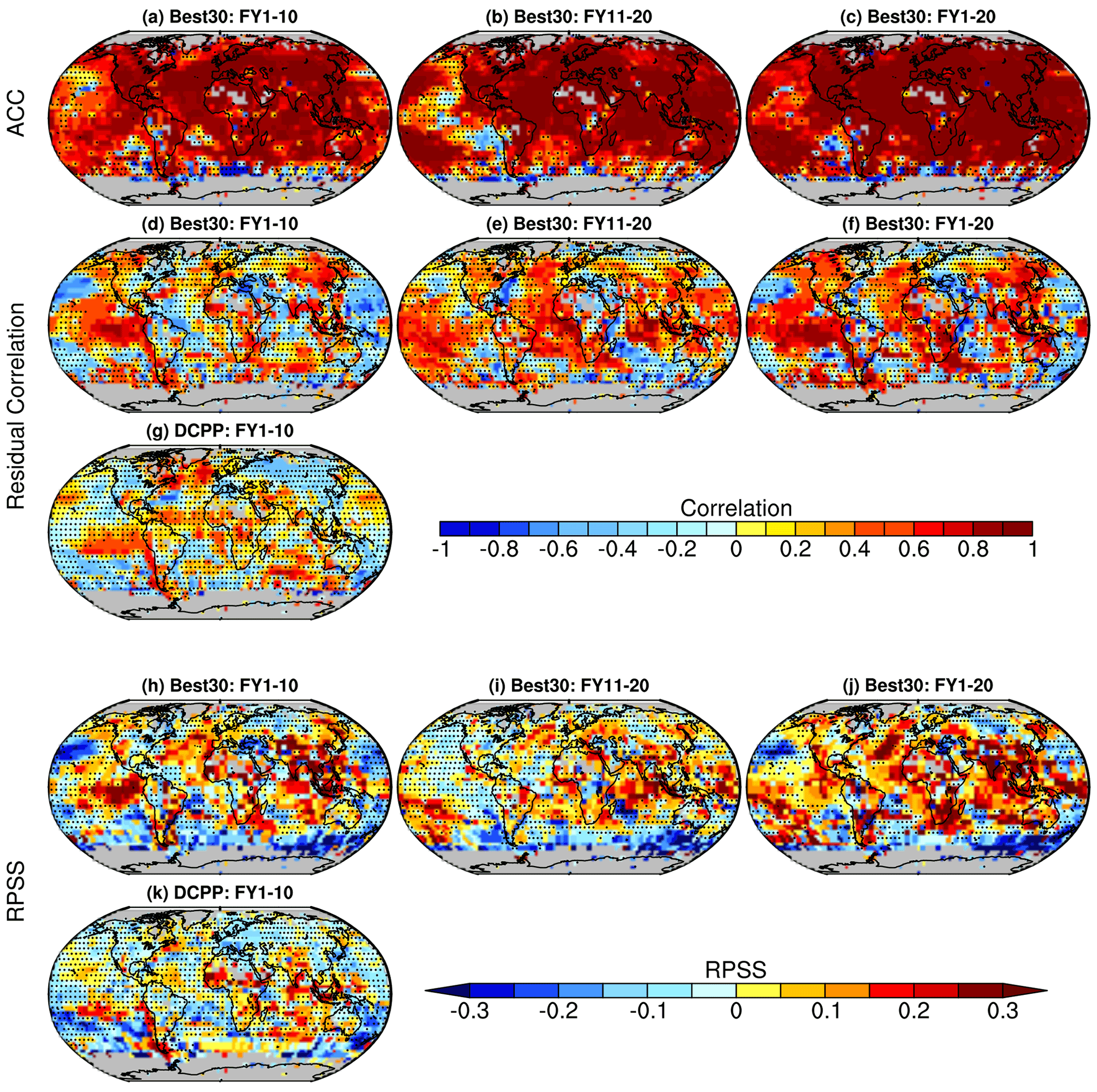
Figure 2Anomaly correlation coefficient (ACC) between observed and predicted near-surface temperature anomalies for three forecast periods, average of forecast years 1–10, 11–20, and 1–20 (a–c). Residual correlations for Best30 (d–f) and for DCPP (g) ensemble means after removing the forced signal (estimated based on ensemble mean of the unconstrained 212 members following Smith et al., 2019). RPSS for Best30 (h–j) and for DCPP (k) against the unconstrained CMIP6 ensemble as reference. Stippling indicates regions where the ACC, residual correlation, and RPSS are statistically not significant at 95 % confidence level (see Methods for details).
Figure 2a–c shows that the Best30 ensemble has high skill in terms of ACC for near-surface air temperature over most of the global regions except in parts of the Pacific and Southern Ocean where the skill is statistically not significant (p>0.05). Similarly high positive ACC values are obtained for the unconstrained ensemble mean (Fig. S1a–c in the Supplement) suggesting that the external forcing signal strongly contributes to these high correlations. To understand the additional skill of the Best30 over the unconstrained ensemble, residual correlations are shown in Fig. 2d–f after removing an estimate of the global warming signal from both the Best30 ensemble and the observations following the methodology of Smith et al. (2019). The same procedure is applied to evaluate the skill of the DCPP ensemble over the unconstrained ensemble for FY1–10 (Fig. 2g).
The results show that the Best30 residual correlations for the first decade are generally similar to DCPP in terms of the overall spatial distributions (cf. Fig. 2d and g). The Best30, however, shows larger added skill than DCPP in many regions including extended areas of the tropical Pacific, parts of Africa, eastern Asia, southern Europe, and Southeast Asia with residual correlations exceeding 0.6. In contrast, DCPP shows higher residual correlations than Best30 in the subpolar North Atlantic, which is a region where previous studies have reported the largest added value in initialized decadal predictions (Doblas-Reyes et al., 2013; Yeager et al., 2018; Smith et al., 2019). Note that higher skill in the North Atlantic can also be achieved for the Best30 when constraining the projections using regional SST anomalies (see Sect. 3.3). Significant added value of the variability-constraint is also found beyond the first 10 forecast years typically covered by decadal predictions. We find positive residual correlations also for FY11–20 (Fig. 2e) and FY1–20 (Fig. 2d) over large parts of the Pacific, Atlantic, and Indian oceans and some neighboring land regions including parts of Africa, Australia, eastern Asia, and North America.
We further evaluate the efficacy of the constraining approach by means of the RPSS where positive values indicate superiority of the Best30 or DCPP over the unconstrained ensemble in making probabilistic forecasts (Fig. 2h–k). Similar to residual correlations, the Best30 shows significant added value over the unconstrained ensemble, and in several regions stronger added value than DCPP, for FY1–10, for example in the eastern tropical Pacific, the North Atlantic, and Indian Ocean, and neighboring land regions in most continents. Significant added value in terms of RPSS is also found for the longer forecast times, e.g., the second decade (FY11–20; Fig. 2i) and the next 20-years (FY1–20; Fig. 2j), over substantial parts of the global ocean and land regions. While many regions consistently exhibit added value from the constraint for the different forecast times shown, in other regions such as large parts of the Atlantic Ocean or the tropical Indian Ocean, positive residual correlations emerge only in the second decade of the hindcasts.
We compare the regional time series from the different ensembles and observations for some selected regions where the constraint adds skill, such as the eastern tropical Pacific, the North Atlantic, and eastern Asia (Fig. S2). These time series show that added skill in the constrained ensemble is often associated with showing a stronger warming rate than the unconstrained CMIP6 ensemble and also DCPP during the first 1–2 investigated decades (e.g., 1961 to 1980 in FY1–10) in these regions, more similar to the observed trend. In some cases (e.g., FY1–20 predictions in eastern Asia and the North Atlantic), the constrained ensemble also better captures the decreased warming rates observed after about 1990. This suggests that added skill in the constrained ensemble is associated with better capturing observed long-term regional warming rates and also decadal-scale variations, whereas the unconstrained CMIP6 ensemble shows a more monotonic warming.
While the focus of this study is on constraining climate variability to improve projection information on decadal to multi-decadal timescales, added value is also evident for shorter forecasting periods. For example, considering the 5-year forecasting periods FY1–5, FY6–10, FY11–15, and FY16–20 (Figs. S3 and S4), we can see that, even if substantial parts of the globe show added value for the different forecast periods, their spatial distribution changes with time. During the first 5 forecast years, the largest added skill is found in the North Atlantic and the eastern tropical Pacific, which evolves to larger parts of the North Pacific during the second pentad (years 6–10). During the third pentad (years 11–15), positive residual correlations are found over large parts of the North Pacific, the Atlantic, and the Indian Ocean, including some adjacent land regions. During the fourth pentad (years 16–20), positive residual correlations remain over large parts of the Atlantic, the Indian Ocean, and some extra-tropical regions of the Pacific Ocean.
The constrained projections also show significant added value in predicting other variables than temperature, for example sea level pressure (Fig. 3). ACC values up to 0.8 and higher are obtained predominantly over the Pacific and the Atlantic oceans, parts of Northern Europe and Asia, the Southern Ocean, and Antarctica (Fig. 3a–c). We again find added value in terms of ACC difference and RPSS over similar regions where also DCPP shows added value during FY1–10, mainly over the tropical Pacific and parts of the Atlantic Ocean. Also for SLP, areas of added skill are found beyond the first decade covered by DCPP, mostly over parts of the Pacific and Atlantic oceans – indicating some SLP predictability on multi-decadal timescales. Some added skill also emerges only in the second forecast decade e.g., over parts of the subtropical Atlantic and the Indian Ocean (noting however that ACC over the Indian Ocean remains negative for all forecast periods shown).
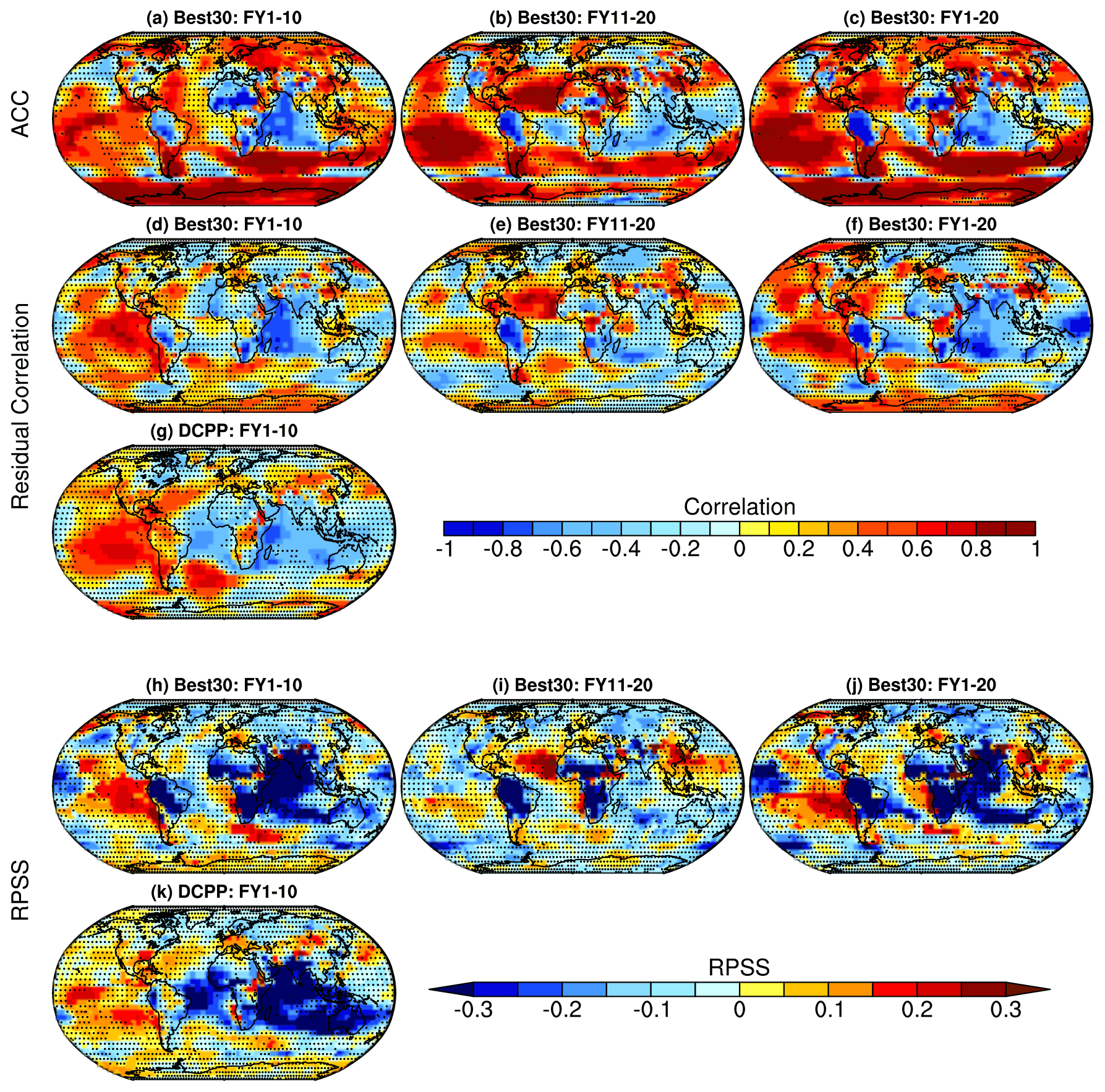
Figure 3Anomaly correlation coefficient (ACC) between observed and predicted SLP anomalies for three forecast periods, average of forecast years 1–10, 11–20, and 1–20 (a–c). Residual correlations for Best30 (d–f) and for DCPP (g) ensemble means after removing the forced signal (estimated based on ensemble mean of the unconstrained 212 members following Smith et al., 2019). RPSS for Best30 (h–j) and for DCPP (k) against the unconstrained CMIP6 ensemble as reference. Stippling indicates regions where the ACC, residual correlation, and RPSS are statistically not significant at 95 % confidence level (see Methods for details).
The constrained projections also show some skill in predicting annual mean precipitation in land areas (Fig. 4). While we find significant skill in terms of ACC over large continental areas (e.g., northern Eurasia, subtropical Africa, and South America, Fig. 4a–c), the added value for the Best30 compared to the unconstrained ensemble, as shown by their ACC difference (Fig. 4d–f), is however generally small. Despite this lack of widespread added value, in some locations such as the Middle East, southern Africa, Australia, and North and South America, the ACC difference is positive and statistically significant at 95 % confidence level for all three forecast periods. Note that also the DCPP-initialized decadal predictions show only small added value for precipitation, and again there is some resemblance in the global patterns of added skill between Best30 and DCPP for FY1–10. Similarly, Best30, as well as DCPP, show limited added value over the unconstrained ensemble in terms of RPSS.
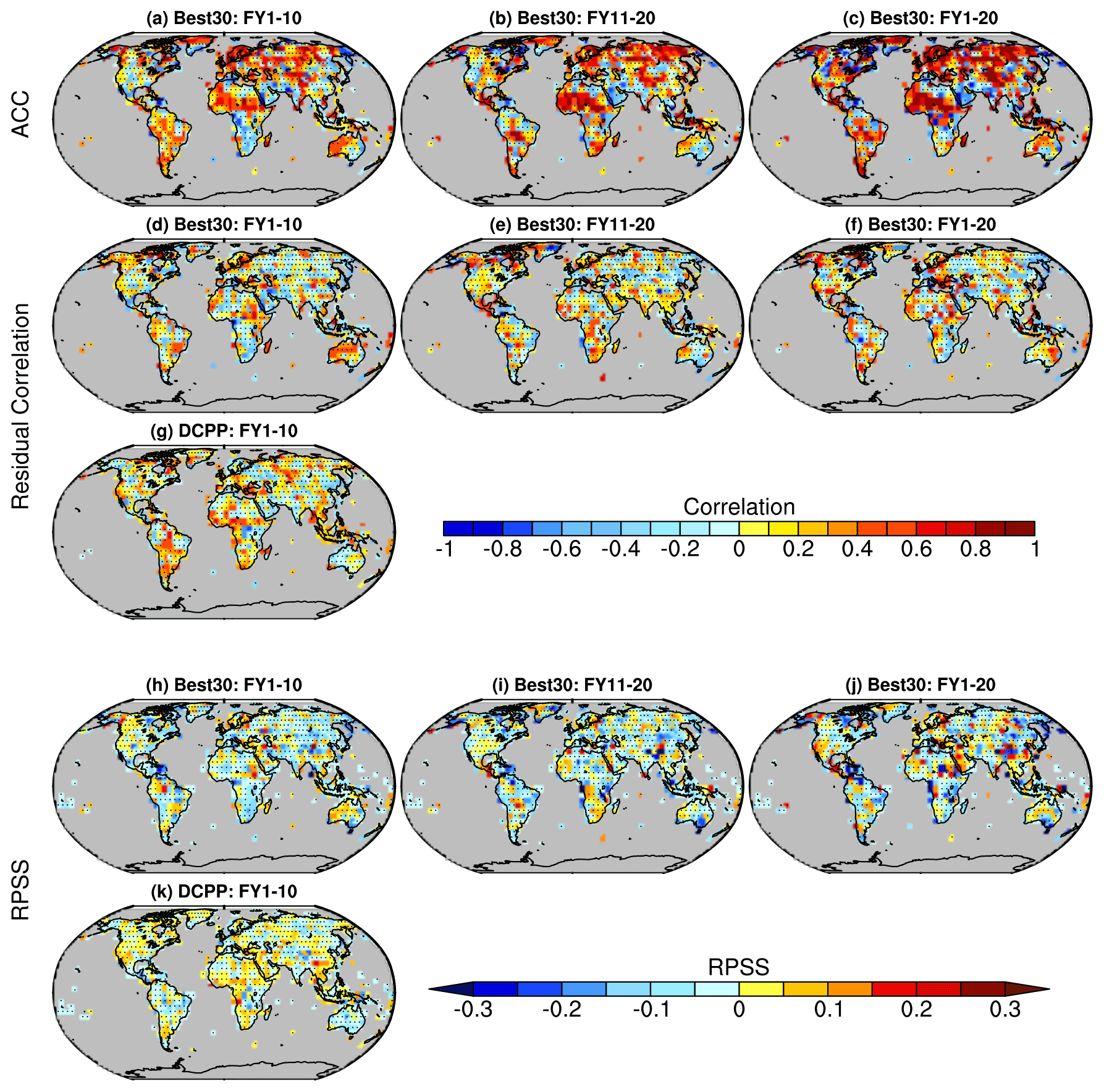
Figure 4Anomaly correlation coefficient (ACC) between observed and predicted precipitation anomalies for three forecast periods, average of forecast years 1–10, 11–20, and 1–20 (a–c). Residual correlations for Best30 (d–f) and for DCPP (g) ensemble means after removing the forced signal (estimated based on ensemble mean of the unconstrained 212 members following Smith et al., 2019). RPSS for Best30 (h–j) and for DCPP (k) against the unconstrained CMIP6 ensemble as reference. Stippling indicates regions where the ACC, residual correlation, and RPSS are statistically not significant at 95 % confidence level (see Methods for details).
3.2 Sensitivity to different selection criteria
We next evaluate the sensitivity of the constrained projections to a number of choices related to the constraining criteria. There is a wide range of choices involved when applying the constraints, and it is beyond the scope of this paper to systematically document all possible choices and their effects. We rather aim to illustrate how different settings can be useful to optimize the results depending on the targeted outcome. In particular we illustrate the sensitivity to (i) the temporal averaging of SST anomalies used for constraining, (ii) the number of ensemble members kept in the constrained ensemble, and (iii) the metric based on which the “best” members are selected.
Figures S5 and S6 show residual correlation and RPSS results, respectively, when selecting the Best30 members using SST anomalies for different time periods instead of using 9-year mean SST anomalies. When selecting based on shorter time averages (e.g., 1 or 3 years), the added value of the constrained ensemble is smaller for decadal and multi-decadal predictions when compared to using longer averages (e.g., 9 years in Fig. 2). The overall spatial patterns of the residual correlations and RPSS are similar between the different selection periods, but values are lower and often not statistically significant when averaging over shorter periods. When using 6-year averages (Figs. S5g–i and S6g–i), results are very similar to our default option of using 9-year averages. These results are also summarized in Fig. 5, where constraints based on 6- and 9-year average SST fields show larger global areas with significant added skill compared to constraints using shorter averaging periods. This suggests that low-frequency variability relevant for decadal to multi-decadal predictions is well constrained when using averages of 6 years or longer. However, the optimal choice for the averaging period depends on the particular prediction target. While averaging over 6 to 9 years is suitable to constrain low-frequency variability and provides added value to predict the next decades, shorter time averages (filtering e.g., for inter-annual variability) can provide larger added value to predict just the next year, as illustrated in Fig. S7. This is plausible as shorter averaging periods will emphasize the signals related to inter-annual variability in the member selections, whereas longer averaging periods will emphasize signals related to lower frequency variability relevant for predicting variations on decadal timescales. Constraints based on 1-year averages lead to significant added value, measured in both residual correlation and RPSS, for forecast year 1 in the tropical Pacific, Indian Ocean, parts of Africa, and Southeast Asia. In contrast, constraints based on averaging SST anomalies over 3 or more years yield almost no added value for forecast year 1. While significant added skill is found for forecast year 1 when constraining based on 1-year SST anomalies, the added skill is smaller than in the initialized DCPP predictions for this same forecast time.
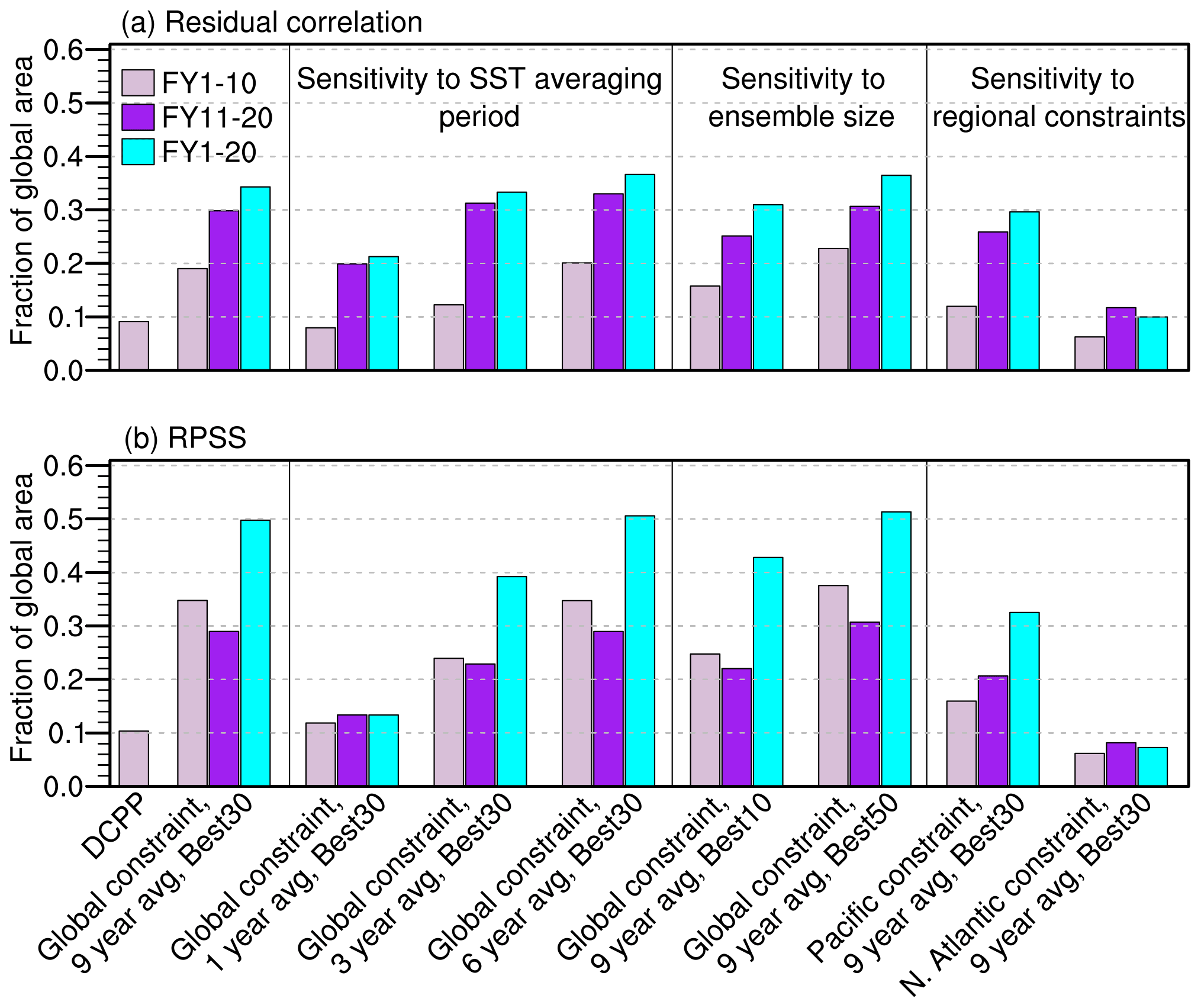
Figure 5Fraction of global area where the added skill in near-surface temperature (measured as residual correlation and RPSS against the unconstrained CMIP6 ensemble as reference) of DCPP and the constrained ensembles is positive and statistically significant at the 95 % confidence level for residual correlation (a) and for RPSS (b). Different colors represent different forecast periods.
Another choice is the number of ensemble members selected for the constrained ensemble. While for initialized climate predictions the benefit of using very large ensembles has been highlighted recently (Smith et al., 2020), the nature of our constraining method implies that simulations in less good agreement with the observed state would be included when selecting more members. In this context, the choice related to the number of selected ensemble members includes a balance between selecting only a few members more closely resembling the observed initial state or a larger constrained ensemble (which could more efficiently capture the predictable signal) that, however, also includes members with decreasing similarity of the initial SST anomaly patterns. The effects of this choice are illustrated in Figs. S8 and S9, where we show the results for selecting the best 10 and best 50 members, respectively. The results indicate overall a high robustness of the results to the number of selected members. All constrained sub-ensembles (of 10, 30, and 50 members) show very similar skill patterns, and added value in similar regions. The magnitude of the added skill (in particular for RPSS) is in some regions slightly larger for the smaller Best10 ensemble, however larger areas with significant added skill are found when using the Best50 ensemble (Fig. S9).
We finally test the use of a different metric to determine the level of agreement between the SST anomaly patterns in observations and the full set of CMIP6 ensemble members. Instead of calculating the pattern correlations, we use the area-weighted root mean squared error (RMSE), calculated based on the differences between observed and simulated SST anomalies over all grid cells (Fig. S10). Again we find broadly similar patterns of skill and added value compared to the “default” approach of constraining based on pattern correlations for 9-year average anomalies. This illustrates that using a globally aggregated error measure can also be useful to select the members in closest agreement with observed variability patterns. However, in our applications we find that the added skill with this alternative selection method is overall smaller than selecting based on pattern correlations. While we do not exclude the possibility that selecting based on RMSE can be advantageous for specific prediction targets, in our applications we find the selections based on pattern correlations to yield higher skill.
3.3 Regional SST constraints and attribution of skill to specific ocean regions
All results discussed so far were for constraints using global SST anomaly patterns, however constraining based on regional SST anomaly patterns can also be useful, either to optimize the skill over specific target regions or to understand the predictive roles of certain ocean basins. Selecting the Best30 based on different SST regions can provide added value to regional scale projections of near-term climate. This is shown by constraining the Best30 ensemble using alternatively SST anomalies from the Pacific (65∘ N–50∘ S) basin or the North Atlantic (0–60∘ N) basin (Figs. S11 and S12). These results show that Pacific constraints lead to substantially larger areas with significant added value than the Atlantic constraints (Fig. S11), with values that are similar to those obtained with the global constraints, which suggests that the Pacific Ocean is a dominant internal predictability source on decadal to multi-decadal timescales (compare Figs. S11, S12, and 2). Constraining based on North Atlantic SSTs, however, provides improved skill of the Best30 over mostly the sub-polar North Atlantic (Figs. S11 and S12) which is not seen when selecting based on either global or Pacific SSTs. Selecting based on Atlantic SSTs also provides some added value on multi-decadal timescales in parts of the Pacific, but overall the global areas with added skill over the unconstrained projections ensemble are smaller than when selecting based on Pacific or global SST anomalies (Fig. 5). We demonstrate here the effects of constraining based on different ocean basins for the global picture of decadal to multi-decadal predictability. Using other more confined ocean regions, ideally physically informed, can thus be useful to optimize skill for specific locations or target regions (e.g., Borchert et al., 2021).
Selecting the “best” members based on regional SSTs can further be useful to attribute predictability to specific ocean regions, and thereby help generate understanding of the climate system. We illustrate this in the following for reproducing the historical evolution of global average temperatures. Observed global average temperatures showed a slowdown in their warming rate during the early 2000s (Fig. 6), sometimes also termed as the “hiatus” period (Easterling and Wehner, 2009; Cowtan and Way, 2014; Trenberth, 2015; Fyfe et al., 2016). The HadCRUT4.6 time series shows a trend slope that is close to zero during 2003-2013, although the true global warming rate is thought to have been slightly larger when accounting for unsampled regions (Cowton and Way, 2014). Some previous studies also identified contributions from natural forcing by moderate volcanic eruptions in the early 2000s to the slowdown in global warming (e.g., Haywood et al., 2014; Ridley et al., 2014; Santer et al., 2014). However, no such warming slowdown is found in the ensemble mean of all CMIP6 projections (which show an increase of 0.2 K per decade during 2003–2013), indicating that forcing is unlikely to explain the reduced global warming rates during that time. The Best30 predictions “initialized” in 1998 (i.e., constrained based on their SST anomaly patterns during 1989–1997) based on global SST patterns show a reduced warming rate of 0.13 K per decade. And constraining based on Pacific SST yields an even smaller warming of about 0.10 K per decade during 2003–2013, confirming the important role of Pacific internal variability in modulating the “hiatus” (Kosaka and Xie, 2013; England et al., 2014).
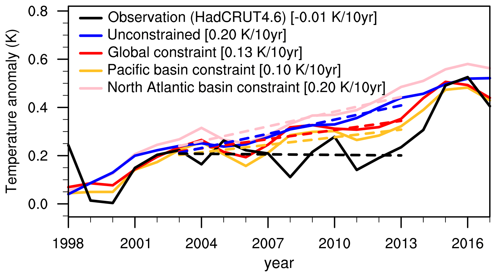
Figure 6Global annual average temperature time series for the period including the global warming “slowdown” in the early 2000s (a). HadCRUT4.6 observational time series (black), the unconstrained/uninitialized projections (blue), and the Best30 ensembles “initialized” in 1998 (i.e., according to the SST anomaly patterns during 1989–1997) constrained based on global (red), Pacific basin (orange), and North Atlantic basin (pink) SST anomaly patterns. The dashed lines show the linear trends during 2003–2013 with corresponding slope values in square brackets after each dataset name in the legend.
Our results further indicate that a reduced global warming rate during the 1.5 decades following 1998 would have been predictable based on the Pacific Ocean temperatures in the preceding decade. No reduced warming rate is found for the Best30 ensemble constrained based on North Atlantic SSTs, suggesting that the North Atlantic did not contribute to this early 2000s global warming slowdown. Note that, also considering the entire hindcast period, the North Atlantic constraint does not improve GMST predictions compared to the full unconstrained ensemble (i.e., residual correlations are negative, not shown). This suggests that, at least based on the models used, the North Atlantic does not seem to provide predictability for global mean temperature. These results add to Risbey et al. (2014), who demonstrated that CMIP5 simulations sub-selected to more closely resemble the concurrent SST trends in the tropical Pacific also showed a slowdown in global warming. However, our results further highlight that such reduced global warming was predictable based on the SSTs prior to 1998.
We present a novel approach to constrain decadal-scale variability in large climate projection ensembles, acting as a poor man's initialization to align the phases of simulated and observed climate variability. The constraint selects those ensemble members most closely resembling observed patterns of multi-annual SST anomalies. We apply this constraint to each year from 1961 onwards to build a set of annually initialized hindcasts that cover multiple decades (i.e., as long as the projection simulations are run). We evaluate the forecast quality of these constrained projections for the following 20 years after applying the annual constraints, focusing the evaluation on the average of forecast years 1–10 (i.e., the forecast period also covered by initialized decadal hindcasts e.g., from DCPP), 11–20, and 1–20. For all these forecast times, the constrained ensemble provides skillful predictions of near-surface temperature, sea-level pressure, and precipitation in large areas of the globe. Significant improvements over the unconstrained ensemble are found in particular for near-surface temperature and sea-level pressure.
The skill of the variability-constrained projections for predicting the first decade is comparable to the skill provided by the DCPP decadal hindcasts. In particular for near-surface temperature, the constrained ensemble provides added skill over the unconstrained large ensemble of projections in larger global areas than DCPP, in particular in the Pacific, where initialized decadal prediction systems tend to have problems (see e.g., Yeager et al., 2018). This indicates that there is decadal-scale predictability in the climate system that is missed by current initialized decadal prediction systems which typically suffer from initialization-related effects perturbing the model attractors, such as shocks and drifts (see e.g., Bilbao et al., 2021). The poor man's initialization, by selecting well spun-up projection members that are in phase with observed variability, does not involve such perturbation of the model attractor, and therefore does not introduce such artifacts. Furthermore, while initialized decadal predictions require large computational resources, the poor man's initialization presented here makes use of existing climate projections and does not require to run any additional simulations.
The added skill in the constrained projections likely comes in part from an improved representation of long-term changes in response to forcing (as also found for decadal predictions, e.g., Doblas-Reyes et al., 2013), and also the representation of decadal-scale variations. Inspection of regional average time series in regions with added skill (e.g., in the Pacific, eastern Asia, or the North Atlantic) indicates warming trends more similar to the observations in the constrained ensemble compared to the full CMIP6 ensemble in particular in the early parts of the hindcast period. These time series also show that the constrained ensemble better captures the observed variations around the warming trend, likely in relation to decadal-scale climate variability.
Constraining against observed SSTs also allows to produce hindcast sets covering much longer time periods (as far back as suitable SST observations are available to make the constraints). Here we start the hindcasts in 1961 for comparability with DCPP. It would also be relatively straightforward to use the presented approach to provide predictions in near-real time (https://hadleyserver.metoffice.gov.uk/wmolc/, last access: October 2022). Such predictions can be done as soon as observational SST fields are available and can also be used as a benchmark for operational decadal prediction.
While initialized climate predictions such as those in DCPP are typically restricted to predictions of the next 10 years after initialization, the predictions based on constrained projections can easily (i.e., at no extra cost) provide climate information beyond 10 years. We identify significant added value from the variability constraint also in the second predicted decade (e.g., forecast years 1–20), and when predicting multi-decadal averages (e.g., forecast years 1–20). These results indicate that there is significant multi-decadal predictability from internal climate variability, which can be exploited to improve near-term climate change estimates.
In this study we discuss some sensitivity of the results to different choices when implementing the constraint, in particular to the averaging time, to the size of the constrained ensemble, to the ocean regions used to evaluate the agreement between models and observations, and to the metric to quantify agreement. These choices can lead to increased or decreased skill for specific regions and prediction timescales. The sensitivity tests therefore also indicate the possibility to optimize the skill for specific applications, e.g., finding the settings that lead to the highest forecast quality for a specific forecast time at a specific location.
We further demonstrate that constraining variability in climate projections can be useful to attribute predictability to certain ocean regions, and thus helps generate understanding of the climate system. By applying the constraint only to certain ocean regions, we can evaluate the regionally constrained ensembles in their ability to predict certain climate phenomena. On the example of the so-called “hiatus” in global mean temperature increases in the early 2000s, we demonstrate that the projections constrained to observed climate anomalies leading up to 1998 are capable of predicting a slowdown in global warming rates during the following 15 years. This predictability can be attributed to constraining Pacific variability (in agreement with previous studies based on specific model experiments prescribing aspects of Pacific variability, such as Kosaka and Xie, 2013 and England et al., 2014).
Our implementation of the constraint to the CMIP6 multi-model ensemble does not select all models with equal probability, and in particular different members of the CanESM5 model (which provides 25 ensemble members) are selected most frequently for many start dates (Fig. S13). This suggests that part of the added skill could come from selecting models better representing some aspects of observed climate. However, we also tested our constraint with an additional condition that limits the number of ensemble members that can be selected from any one model respectively to three or five members at each start date – forcing the method to select members more evenly across models. This condition leads to overall slightly reduced skill, but very similar patterns of skill (Fig. S14), indicating that a substantial part of the skill does not depend on the specific models selected and that constraining decadal-scale variability is an important contributor to skill. Still, there may be important challenges when applying the approach to actually predict future climate, related for example to unrealistically high climate sensitivity of some CMIP6 models (Zelinka et al., 2020). For applications to future climate prediction it might therefore be useful to pre-filter the multi-model ensemble, excluding those with unrealistically high climate sensitivity (Hausfather et al., 2022).
Analogue-based selections of climate simulations have been proven useful in the context of both seasonal and regional decadal predictions (Ding et al., 2018; Menary et al., 2021). Using SST and sea surface height anomalies, and selecting those simulations with minimum distance to the target climate states, Ding et al. (2018) demonstrated skill of such sub-selected analogues in predicting observed monthly mean SST and sea surface height anomalies mainly in the tropical Indo-Pacific region over the following 12 months. Menary et al. (2021) used a pool of 35-year mean SST anomalies from different CMIP5 and CMIP6 experiments to find model analogues with the lowest error in spatial patterns compared to observed states of 35-year mean SST anomalies, to make predictions for years 2–10 in the North Atlantic region. They found the analogue-based predictions (selecting from uninitialized simulations) to have comparable skill to the initialized predictions of SSTs in the North Atlantic sub-polar gyre region.
The constraining approach used here is similar to Mahmood et al. (2021), who constrained a 40-member single-model ensemble based on the pattern agreement with initialized decadal predictions. The major differences are that here we select members from a much larger multi-model ensemble, and we select based on the agreement with SST anomaly patterns from observations instead of decadal predictions. The benefit from the constraint (in terms of added skill) found here is substantially larger than reported by Mahmood et al. (2021), likely due to the large ensemble size of CMIP6 projections to select from. Also, constraining based on decadal predictions requires that these decadal predictions add skill over the projections, which only happens in certain regions like the North Atlantic (Befort et al., 2020). Limitations that deteriorate the skill in decadal predictions (e.g., Bilbao et al., 2021) may however transfer to the constrained projections. Future work will test the decadal predictions-based constraint on the large multi-model ensemble of projections as used here to understand if the larger ensemble size also benefits that approach.
Both approaches, constraining the projections based on their agreement with either observations or decadal predictions, can be used to provide seamless climate information for the next multiple decades. This is an important advantage over the use of different datasets for different timescales, e.g., initialized seasonal to decadal predictions for the first few years and projections afterwards. Data from these different sources are often inconsistent, both in a statistical sense and the climate conditions that they represent. In contrast, the variability-constrained projections provide consistent transient climate information for the next years and multiple decades, which can facilitate their use when seamless climate information across timescales is required. We show here that such constrained projections show promising skill, comparable to initialized predictions on the decadal timescale, and provide significant added value over unconstrained projections on multi-decadal timescales – pointing to predictability in the climate system that is not currently exploited with existing prediction systems. The variability-constrained projections therefore provide a promising pathway to provide improved climate information, of reduced uncertainty and increased accuracy, about near-term climate change in the next few decades. This improved information can be useful to underpin targeted adaptation strategies.
CMIP6 data are available through various ESFG data nodes (https://www.wcrp-climate.org/wgcm-cmip/wgcm-cmip6; WCRP, 2022). Other data sets used in this study are also available from their respective data sources:
-
ERSST: https://psl.noaa.gov/data/gridded/data.noaa.ersst.v5.html (NOAA, 2022a);
-
HadCRUT: https://crudata.uea.ac.uk/cru/data/temperature/ (Climate Research Unit, 2022a);
-
CRU precipitation: https://crudata.uea.ac.uk/cru/data/hrg/ (Climate Research Unit, 2022b);
-
GPCC: https://www.dwd.de/EN/ourservices/gpcc/gpcc.html (DWD, 2022);
-
ERA5: https://www.ecmwf.int/en/forecasts/datasets/reanalysis-datasets/era5 (ECMWF, 2022);
-
JRA55: https://jra.kishou.go.jp/JRA-55/index_en.html (JRA project, 2022);
-
NOAAGlobTemp: https://www.ncei.noaa.gov/access/monitoring/global-temperature-anomalies/grid (NOAA, 2022b).
The supplement related to this article is available online at: https://doi.org/10.5194/esd-13-1437-2022-supplement.
MGD, PO, FJDR, and RM designed the study. RM performed the analysis with active guidance from MGD, PO, and FJDR. RM and MGD drafted the paper. CDT helped with the probabilistic forecast quality assessment. MS and PAB downloaded and managed the large datasets of CMIP6 simulations and the observations. All authors contributed to the writing.
The contact author has declared that none of the authors has any competing interests.
Publisher's note: Copernicus Publications remains neutral with regard to jurisdictional claims in published maps and institutional affiliations.
We acknowledge the World Climate Research Programme, which, through its Working Group on Coupled Modelling, coordinated and promoted CMIP6. We thank the climate modeling groups for producing and making available their model output, the Earth System Grid Federation (ESGF) for archiving the data and providing access, and the multiple funding agencies who support CMIP6 and ESGF.
This research has been funded by the Spanish Science and Innovation Ministry (project PATHFINDER; grant no. PID2021-127943NB-I00) and the European Commission (Horizon 2020 project EUCP; grant no. 776613). Markus G. Donat and Pablo Ortega were funded by the Spanish Ministry for Science and Innovation grant references RYC-2017-22964 and RYC-2017-22772, respectively. Markus G. Donat was supported by the AXA Research Fund. Carlos Delgado-Torres received financial support from the Spanish Ministry for Science and Innovation (FPI PRE2019-509 08864 financed by MCIN/AEI/10.13039/501100011033 and by FSE invierte en tu futuro).
This paper was edited by Gabriele Messori and reviewed by three anonymous referees.
Befort, D. J., O'Reilly, C. H., and Weisheimer, A.: Constraining Projections Using Decadal Predictions, Geophys. Res. Lett., 47, e2020GL087900, https://doi.org/10.1029/2020GL087900, 2020.
Bilbao, R., Wild, S., Ortega, P., Acosta-Navarro, J., Arsouze, T., Bretonnière, P.-A., Caron, L.-P., Castrillo, M., Cruz-García, R., Cvijanovic, I., Doblas-Reyes, F. J., Donat, M., Dutra, E., Echevarría, P., Ho, A.-C., Loosveldt-Tomas, S., Moreno-Chamarro, E., Pérez-Zanon, N., Ramos, A., Ruprich-Robert, Y., Sicardi, V., Tourigny, E., and Vegas-Regidor, J.: Assessment of a full-field initialized decadal climate prediction system with the CMIP6 version of EC-Earth, Earth Syst. Dynam., 12, 173–196, https://doi.org/10.5194/esd-12-173-2021, 2021.
Boer, G. J., Smith, D. M., Cassou, C., Doblas-Reyes, F., Danabasoglu, G., Kirtman, B., Kushnir, Y., Kimoto, M., Meehl, G. A., Msadek, R., Mueller, W. A., Taylor, K. E., Zwiers, F., Rixen, M., Ruprich-Robert, Y., and Eade, R.: The Decadal Climate Prediction Project (DCPP) contribution to CMIP6, Geosci. Model Dev., 9, 3751–3777, https://doi.org/10.5194/gmd-9-3751-2016, 2016.
Borchert, L. F., Koul, V., Menary, M. B., Befort, D. J., Swingedouw, D., Sgubin, G., and Mignot, J.: Skillful decadal prediction of unforced southern European summer temperature variations, Environ. Res. Lett., 16, 104017, https://doi.org/10.1088/1748-9326/ac20f5, 2021.
Climate Research Unit: Temperature, Climate Research Unit [data set], https://crudata.uea.ac.uk/cru/data/temperature/ (last access: October 2022), 2022a.
Climate Research Unit: High-resolution gridded datasets (and derived products), Climate Research Unit [data set], https://crudata.uea.ac.uk/cru/data/hrg/ (last access: October 2022), 2022b.
Cowtan, K. and Way, R. G.: Coverage bias in the HadCRUT4 temperature series and its impact on recent temperature trends, Q. J. Roy. Meteorol. Soc., 140, 1935–1944, https://doi.org/10.1002/qj.2297, 2014.
DelSole, T. and Tippett, M. K.: Forecast Comparison Based on Random Walks, Mon. Weather Rev., 144, 615–626, https://doi.org/10.1175/MWR-D-15-0218.1, 2016.
Ding, H., Newman, M., Alexander, M. A., and Wittenberg, A. T.: Skillful Climate Forecasts of the Tropical Indo-Pacific Ocean Using Model-Analogs, J. Climate, 31, 5437–5459, https://doi.org/10.1175/JCLI-D-17-0661.1, 2018.
Doblas-Reyes, F. J., Andreu-Burillo, I., Chikamoto, Y., García-Serrano, J., Guemas, V., Kimoto, M., Mochizuki, T., Rodrigues, L. R. L., and van Oldenborgh, G. J.: Initialized near-term regional climate change prediction, Nat. Commun., 4, 1715, https://doi.org/10.1038/ncomms2704, 2013.
DWD: GPCC, DWD [data set], https://www.dwd.de/EN/ourservices/gpcc/gpcc.html, last access: October 2022.
Easterling, D. R. and Wehner, M. F.: Is the climate warming or cooling?, Geophys. Res. Lett., 36, L08706, https://doi.org/10.1029/2009GL037810, 2009.
ECMWF: ERA5, ECMWF [data set], https://www.ecmwf.int/en/forecasts/datasets/reanalysis-datasets/era5, last access: October 2022.
England, M. H., McGregor, S., Spence, P., Meehl, G. A., Timmermann, A., Cai, W., Gupta, A. S., McPhaden, M. J., Purich, A., and Santoso, A.: Recent intensification of wind-driven circulation in the Pacific and the ongoing warming hiatus, Nat. Clim. Change, 4, 222–227, https://doi.org/10.1038/nclimate2106, 2014.
Eyring, V., Bony, S., Meehl, G. A., Senior, C. A., Stevens, B., Stouffer, R. J., and Taylor, K. E.: Overview of the Coupled Model Intercomparison Project Phase 6 (CMIP6) experimental design and organization, Geosci. Model Dev., 9, 1937–1958, https://doi.org/10.5194/gmd-9-1937-2016, 2016.
Fyfe, J. C., Meehl, G. A., England, M. H., Mann, M. E., Santer, B. D., Flato, G. M., Hawkins, E., Gillett, N. P., Xie, S.-P., Kosaka, Y., and Swart, N. C.: Making sense of the early-2000s warming slowdown, Nat. Clim. Change, 6, 224–228, https://doi.org/10.1038/nclimate2938, 2016.
Goddard, L., Kumar, A., Solomon, A., Smith, D., Boer, G., Gonzalez, P., Kharin, V., Merryfield, W., Deser, C., Mason, S. J., Kirtman, B. P., Msadek, R., Sutton, R., Hawkins, E., Fricker, T., Hegerl, G., Ferro, C. A. T., Stephenson, D. B., Meehl, G. A., Stockdale, T., Burgman, R., Greene, A. M., Kushnir, Y., Newman, M., Carton, J., Fukumori, I., and Delworth, T.: A verification framework for interannual-to-decadal predictions experiments, Clim. Dynam., 40, 245–272, https://doi.org/10.1007/s00382-012-1481-2, 2013.
Guemas, V., Auger, L., and Doblas-Reyes, F. J.: Hypothesis Testing for Autocorrelated Short Climate Time Series, J. Appl. Meteorol. Clim., 53, 637–651, https://doi.org/10.1175/JAMC-D-13-064.1, 2014.
Hausfather, Z., Marvel, K., Schmidt, G. A., Nielsen-Gammon, J. W., and Zelinka, M.: Climate simulations: recognize the `hot model' problem, Nature, 605, 26–29, https://doi.org/10.1038/d41586-022-01192-2, 2022.
Hawkins, E. and Sutton, R.: The Potential to Narrow Uncertainty in Regional Climate Predictions, B. Am. Meteorol. Soc., 90, 1095–1108, https://doi.org/10.1175/2009BAMS2607.1, 2009.
Hawkins, E. and Sutton, R.: The potential to narrow uncertainty in projections of regional precipitation change, Clim. Dynam., 37, 407–418, https://doi.org/10.1007/s00382-010-0810-6, 2011.
Haywood, J. M., Jones, A., and Jones, G. S.: The impact of volcanic eruptions in the period 2000–2013 on global mean temperature trends evaluated in the HadGEM2-ES climate model: Impact of modest volcanic eruptions on the global warming trends, Atmos. Sci. Lett., 15, 92–96, https://doi.org/10.1002/asl2.471, 2014.
Hazeleger, W., Guemas, V., Wouters, B., Corti, S., Andreu-Burillo, I., Doblas-Reyes, F. J., Wyser, K., and Caian, M.: Multiyear climate predictions using two initialization strategies, Geophys. Res. Lett., 40, 1794–1798, https://doi.org/10.1002/grl.50355, 2013.
Hegerl, G. C., Ballinger, A. P., Booth, B. B. B., Borchert, L. F., Brunner, L., Donat, M. G., Doblas-Reyes, F. J., Harris, G. R., Lowe, J., Mahmood, R., Mignot, J., Murphy, J. M., Swingedouw, D., and Weisheimer, A.: Toward Consistent Observational Constraints in Climate Predictions and Projections, Front. Clim., 3, 678109, https://doi.org/10.3389/fclim.2021.678109, 2021.
Huang, B., Thorne, P. W., Banzon, V. F., Boyer, T., Chepurin, G., Lawrimore, J. H., Menne, M. J., Smith, T. M., Vose, R. S., and Zhang, H.-M.: Extended Reconstructed Sea Surface Temperature, Version 5 (ERSSTv5): Upgrades, Validations, and Intercomparisons, J. Climate, 30, 8179–8205, https://doi.org/10.1175/JCLI-D-16-0836.1, 2017.
IPCC: Summary for Policymakers, in: Climate Change 2021: The Physical Science Basis, Contribution of Working Group I to the Sixth Assessment Report of the Intergovernmental Panel on Climate Change, edited by: Masson-Delmotte, V., Zhai, P., Pirani, A., Connors, S. L., Péan, C., Berger, S., Caud, N., Chen, Y., Goldfarb, L., Gomis, M. I., Huang, M., Leitzell, K., Lonnoy, E., Matthews, J. B. R., Maycock, T. K., Waterfield, T., Yelekçi, O., Yu, R., and Zhou, B., Cambridge University Press, Cambridge, UK and New York, NY, USA, 3–32, https://doi.org/10.1017/9781009157896.001, 2021.
JRA project: JRA-55 – the Japanese 55-year Reanalysis, https://jra.kishou.go.jp/JRA-55/index_en.html, last access: October 2022.
Kobayashi, S., Ota, Y., Harada, Y., Ebita, A., Moriya, M., Onoda, H., Onogi, K., Kamahori, H., Kobayashi, C., Endo, H., Miyaoka, K., and Takahashi, K.: The JRA-55 Reanalysis: General Specifications and Basic Characteristics, J. Meteorol. Soc. Jpn., 93, 5–48, https://doi.org/10.2151/jmsj.2015-001, 2015.
Kosaka, Y. and Xie, S.-P.: Recent global-warming hiatus tied to equatorial Pacific surface cooling, Nature, 501, 403–407, https://doi.org/10.1038/nature12534, 2013.
Kushnir, Y., Scaife, A. A., Arritt, R., Balsamo, G., Boer, G., Doblas-Reyes, F., Hawkins, E., Kimoto, M., Kolli, R. K., Kumar, A., Matei, D., Matthes, K., Müller, W. A., O'Kane, T., Perlwitz, J., Power, S., Raphael, M., Shimpo, A., Smith, D., Tuma, M., and Wu, B.: Towards operational predictions of the near-term climate, Nat. Clim. Change, 9, 94–101, https://doi.org/10.1038/s41558-018-0359-7, 2019.
Lehner, F., Deser, C., Maher, N., Marotzke, J., Fischer, E. M., Brunner, L., Knutti, R., and Hawkins, E.: Partitioning climate projection uncertainty with multiple large ensembles and CMIP5/6, Earth Syst. Dynam., 11, 491–508, https://doi.org/10.5194/esd-11-491-2020, 2020.
Mahmood, R., Donat, M. G., Ortega, P., Doblas-Reyes, F. J., and Ruprich-Robert, Y.: Constraining Decadal Variability Yields Skillful Projections of Near-Term Climate Change, Geophys. Res. Lett., 48, e2021GL094915, https://doi.org/10.1029/2021GL094915, 2021.
Meehl, G. A., Richter, J. H., Teng, H., Capotondi, A., Cobb, K., Doblas-Reyes, F., Donat, M. G., England, M. H., Fyfe, J. C., Han, W., Kim, H., Kirtman, B. P., Kushnir, Y., Lovenduski, N. S., Mann, M. E., Merryfield, W. J., Nieves, V., Pegion, K., Rosenbloom, N., Sanchez, S. C., Scaife, A. A., Smith, D., Subramanian, A. C., Sun, L., Thompson, D., Ummenhofer, C. C., and Xie, S.-P.: Initialized Earth System prediction from subseasonal to decadal timescales, Nat. Rev. Earth Environ., 2, 340–357, https://doi.org/10.1038/s43017-021-00155-x, 2021.
Menary, M. B., Mignot, J., and Robson, J.: Skilful decadal predictions of subpolar North Atlantic SSTs using CMIP model-analogues, Environ. Res. Lett., 16, 064090, https://doi.org/10.1088/1748-9326/ac06fb, 2021.
Morice, C. P., Kennedy, J. J., Rayner, N. A., and Jones, P. D.: Quantifying uncertainties in global and regional temperature change using an ensemble of observational estimates: The HadCRUT4 data set: The HadCRUT4 data , J. Geophys. Res., 117, D08101, https://doi.org/10.1029/2011JD017187, 2012.
NOAA: NOAA Extended Reconstructed SST V5, NOAA [data set], https://psl.noaa.gov/data/gridded/data.noaa.ersst.v5.html (last access: October 2022), 2022a.
NOAA: Gridded Dataset, NOAA [data set], https://www.ncei.noaa.gov/access/monitoring/global-temperature-anomalies/grid (last access: October 2022), 2022b.
Ridley, D. A., Solomon, S., Barnes, J. E., Burlakov, V. D., Deshler, T., Dolgii, S. I., Herber, A. B., Nagai, T., Neely, R. R., Nevzorov, A. V., Ritter, C., Sakai, T., Santer, B. D., Sato, M., Schmidt, A., Uchino, O., and Vernier, J. P.: Total volcanic stratospheric aerosol optical depths and implications for global climate change: Uncertainty in volcanic climate forcing, Geophys. Res. Lett., 41, 7763–7769, https://doi.org/10.1002/2014GL061541, 2014.
Risbey, J. S., Lewandowsky, S., Langlais, C., Monselesan, D. P., O'Kane, T. J., and Oreskes, N.: Well-estimated global surface warming in climate projections selected for ENSO phase, Nat. Clim. Change, 4, 835–840, https://doi.org/10.1038/nclimate2310, 2014.
Santer, B. D., Bonfils, C., Painter, J. F., Zelinka, M. D., Mears, C., Solomon, S., Schmidt, G. A., Fyfe, J. C., Cole, J. N. S., Nazarenko, L., Taylor, K. E., and Wentz, F. J.: Volcanic contribution to decadal changes in tropospheric temperature, Nat. Geosci., 7, 185–189, https://doi.org/10.1038/ngeo2098, 2014.
Schamm, K., Ziese, M., Becker, A., Finger, P., Meyer-Christoffer, A., Schneider, U., Schröder, M., and Stender, P.: Global gridded precipitation over land: a description of the new GPCC First Guess Daily product, Earth Syst. Sci. Data, 6, 49–60, https://doi.org/10.5194/essd-6-49-2014, 2014.
Smith, D. M., Eade, R., and Pohlmann, H.: A comparison of full-field and anomaly initialization for seasonal to decadal climate prediction, Clim. Dynam., 41, 3325–3338, https://doi.org/10.1007/s00382-013-1683-2, 2013.
Smith, D. M., Eade, R., Scaife, A. A., Caron, L.-P., Danabasoglu, G., DelSole, T. M., Delworth, T., Doblas-Reyes, F. J., Dunstone, N. J., Hermanson, L., Kharin, V., Kimoto, M., Merryfield, W. J., Mochizuki, T., Müller, W. A., Pohlmann, H., Yeager, S., and Yang, X.: Robust skill of decadal climate predictions, npj Clim. Atmos. Sci., 2, 13, https://doi.org/10.1038/s41612-019-0071-y, 2019.
Smith, D. M., Scaife, A. A., Eade, R., Athanasiadis, P., Bellucci, A., Bethke, I., Bilbao, R., Borchert, L. F., Caron, L.-P., Counillon, F., Danabasoglu, G., Delworth, T., Doblas-Reyes, F. J., Dunstone, N. J., Estella-Perez, V., Flavoni, S., Hermanson, L., Keenlyside, N., Kharin, V., Kimoto, M., Merryfield, W. J., Mignot, J., Mochizuki, T., Modali, K., Monerie, P.-A., Müller, W. A., Nicolí, D., Ortega, P., Pankatz, K., Pohlmann, H., Robson, J., Ruggieri, P., Sospedra-Alfonso, R., Swingedouw, D., Wang, Y., Wild, S., Yeager, S., Yang, X., and Zhang, L.: North Atlantic climate far more predictable than models imply, Nature, 583, 796–800, https://doi.org/10.1038/s41586-020-2525-0, 2020.
Taylor, K. E., Stouffer, R. J., and Meehl, G. A.: An Overview of CMIP5 and the Experiment Design, B. Am. Meteorol. Soc., 93, 485–498, https://doi.org/10.1175/BAMS-D-11-00094.1, 2012.
Trenberth, K. E.: Has there been a hiatus?, Science, 349, 691–692, https://doi.org/10.1126/science.aac9225, 2015.
WCRP: CMIP Phase 6 (CMIP6), https://www.wcrp-climate.org/wgcm-cmip/wgcm-cmip6, last access: October 2022.
Wilks, D. S.: Statistical methods in the atmospheric sciences, Elsevier, Amsterdam, the Netherlands, Boston, ISBN 978-0-12-385022-5 978-0-12-385023-2, 2011.
Yeager, S. G., Danabasoglu, G., Rosenbloom, N. A., Strand, W., Bates, S. C., Meehl, G. A., Karspeck, A. R., Lindsay, K., Long, M. C., Teng, H., and Lovenduski, N. S.: Predicting Near-Term Changes in the Earth System: A Large Ensemble of Initialized Decadal Prediction Simulations Using the Community Earth System Model, B. Am. Meteorol. Soc., 99, 1867–1886, https://doi.org/10.1175/BAMS-D-17-0098.1, 2018.
Zelinka, M. D., Myers, T. A., McCoy, D. T., Po-Chedley, S., Caldwell, P. M., Ceppi, P., Klein, S. A., and Taylor, K. E.: Causes of Higher Climate Sensitivity in CMIP6 Models, Geophys. Res. Lett., 47, e2019GL085782, https://doi.org/10.1029/2019GL085782, 2020.