the Creative Commons Attribution 4.0 License.
the Creative Commons Attribution 4.0 License.
 | 06 Sep 2022
Combining machine learning and SMILEs to classify, better understand, and project changes in ENSO events
Thibault P. Tabarin
Sebastian Milinski
The El Niño–Southern Oscillation (ENSO) occurs in three phases: neutral, warm (El Niño), and cool (La Niña). While classifying El Niño and La Niña is relatively straightforward, El Niño events can be broadly classified into two types: central Pacific (CP) and eastern Pacific (EP). Differentiating between CP and EP events is currently dependent on both the method and observational dataset used. In this study, we create a new classification scheme using supervised machine learning trained on 18 observational and re-analysis products. This builds on previous work by identifying classes of events using the temporal evolution of sea surface temperature in multiple regions across the tropical Pacific. By applying this new classifier to seven single model initial-condition large ensembles (SMILEs) we investigate both the internal variability and forced changes in each type of ENSO event, where events identified behave similarly to those observed. It is currently debated whether the observed increase in the frequency of CP events after the late 1970s is due to climate change. We found it to be within the range of internal variability in the SMILEs for trends after 1950, but not for the full observed period (1896 onwards). When considering future changes, we do not project a change in CP frequency or amplitude under a strong warming scenario (RCP8.5/SSP370) and we find model differences in EP El Niño and La Niña frequency and amplitude projections. Finally, we find that models show differences in projected precipitation and sea surface temperature (SST) pattern changes for each event type that do not seem to be linked to the Pacific mean state SST change, although the SST and precipitation changes in individual SMILEs are linked. Our work demonstrates the value of combining machine learning with climate models, and highlights the need to use SMILEs when evaluating ENSO in climate models because of the large spread of results found within a single model due to internal variability alone.
- Article
(10325 KB) - Full-text XML
-
Supplement
(7597 KB) - BibTeX
- EndNote


Understanding El Niño–Southern Oscillation (ENSO) diversity is important due to the differing teleconnections and impacts of different types of events (e.g. Capotondi et al., 2020, and refs therein). ENSO occurs in three phases: neutral, La Niña, and El Niño. While El Niño events occur with a wide range of spatial structures (Giese and Ray, 2011) they can be broadly classified into two types, which differ in evolution, strength, and spatial structure (e.g. Capotondi et al., 2015, 2020). These are eastern Pacific (EP) El Niño and central Pacific (CP) El Niño events. EP El Niño events have warm sea surface temperature (SST) anomalies located in the eastern equatorial Pacific, typically attached to the coastline of South America, while for CP El Niño events SST, wind, and subsurface anomalies are confined to the central Pacific (Kao and Yu, 2009). EP events tend to appear in the far east Pacific and move westward, with CP events generally appearing in the eastern subtropics and central Pacific (Kao and Yu, 2009; Yeh et al., 2014; Capotondi et al., 2015). EP events occur from weak to extremely strong in amplitude, while CP events tend to be on the weaker side (e.g. Capotondi et al., 2020). In this study we use supervised machine learning techniques to create a new classification scheme.
There is ongoing debate about the cause of an observed increase in the frequency of CP events after the late 1970s (An and Wang, 2000). This was initially attributed to increased greenhouse gas forcing (Yeh et al., 2009). Other studies then suggested that multi-decadal modulation of CP frequency by internal variability can explain this increase (McPhaden et al., 2011; Newman et al., 2011; Yeh et al., 2011; Pascolini-Campbell et al., 2015). However, a recent study again suggested that this observed increase can be linked to greenhouse gas forcing (Liu et al., 2017). Additionally, palaeoclimate records have shown that the current ratio of CP to EP El Niño events is unusual in a multi-century context (Freund et al., 2019). Freund et al. (2019) use corals from 27 seasonally resolved networks and find that compared to the last four centuries the recent 30-year period includes fewer but more extreme EP El Niño events and an unprecedented ratio of CP to EP El Niño events compared to the rest of the record. It is currently unresolved why these past changes seen in the palaeoclimate record occurred.
Whether both the frequency and amplitude of EP and CP events will change in the future is also strongly debated. Multiple studies agree that projections are inconsistent across CMIP5 models (Ham et al., 2015; Chen et al., 2017b; Xu et al., 2017; Lemmon and Karnauskas, 2019). These differences are suggested to be related to the central Pacific zonal SST gradient (Wang et al., 2019). When subsetting for models that represent ENSO well, studies find an increase in EP variability (Cai et al., 2018, 2021). However, when using single model initial-condition large ensembles (SMILEs), models are again found to differ in their projections (Ng et al., 2021). ENSO precipitation projections are more robust across all models, with multiple studies projecting an increase in ENSO-related precipitation variability under strong warming scenarios (Power et al., 2013; Cai et al., 2014; Chung et al., 2014; Watanabe et al., 2014; Huang and Xie, 2015; Yun et al., 2021).
While there is a wealth of literature investigating ENSO, previous work has highlighted that due to its high variability longer equilibrated runs or SMILEs are needed to truly understand our observations of ENSO and to project future changes (Wittenberg, 2009; Maher et al., 2018; Milinski et al., 2020). Two separate studies show that two SMILEs cover the spread of ENSO projections in CMIP5 models for both traditional ENSO indices (Maher et al., 2018) and EP and CP events (Ng et al., 2021). This indicates that internal variability can explain a large fraction of the inter-model spread previously attributed to model differences. These results highlight the utility of SMILEs, which provide many realisations of the earth system and allow scientists to investigate both the climate change signal as well as inherently complex and noisy systems such as ENSO (Maher et al., 2018).
Previous studies have used varying methods to classify El Niño events into EP and CP events, but are limited by uncertainty in both the observed data and the classification method. Pascolini-Campbell et al. (2015) summarise nine classification schemes (Ashok et al., 2007; Hendon et al., 2009; Kao and Yu, 2009; Kim et al., 2009; Kug et al., 2009; Ren and Jin, 2011; Takahashi et al., 2011; Yeh et al., 2009; Yu and Kim, 2010) applied to five different SST products and show that event classification is dependent on both the index and dataset used. They identify events that appear with greatest convergence across indices and datasets to provide the most robust classification of observations to date. Such classification using multiple SST products can now be automated using machine learning, which has the additional advantage of using multiple parameters across many dimensions to identify events. This technique provides potential to create a more complete classifier than previous studies, where classification schemes have focused on single metrics with defined thresholds or the comparison of multiple schemes and products by hand (Pascolini-Campbell et al., 2015).
Machine learning techniques such as classification are becoming more commonly utilised in the geosciences. The key challenges in applying machine learning in this field come from the difficulty in establishing ground truth data, interpreting physical results, auto-correlation at both spatial and temporal scales, noisy data with gaps that are taken at multiple resolutions and scales, as well as data that are uncertain, sparse, and intermittent (Gil et al., 2018; Karpatne et al., 2019; Reichstein et al., 2019). Machine learning, however, also provides new opportunities in the geosciences particularly when using climate models where large coherent datasets exist (Barnes et al., 2020, 2019; Toms et al., 2020). Studies have begun to apply such techniques to ENSO research, for example using unsupervised learning and clustering algorithms to identify different types of ENSO events (Wang et al., 2019; Johnson, 2013) and to more reliably predict ENSO (Ham et al., 2019; Guo et al., 2020). However, no studies to date have used supervised learning combined with observations to investigate ENSO. In this study, we use supervised machine learning to build a new ENSO classifier. We then apply this classifier to climate models in order to identify events that resemble those found in the real world. This is relevant as we wish to study events similar to those that we observe.
The aims of this paper are twofold. First, we create a new classifier using supervised machine learning combined with 18 observational and re-analysis products. This classifier has the advantage that it can learn both the spatial and temporal evolution of different events, unlike previous studies that rely on pre-defined metrics and compare multiple methods and products by hand. Second, we apply the classifier to seven SMILEs to answer three questions. (1) Can SMILEs capture the observed CP and EP El Niño events and La Niña events? (2) Can the observed increase in frequency of CP El Niño events be explained by internal variability and what does this imply for future projections? (3) Do we project forced changes in the amplitude, SST, and precipitation patterns of each event type? By using this classifier combined with SMILEs we can now better understand observations and projections of ENSO in the context of internal variability.
The purpose of a classifier is to assign a class to an event. In this paper our intent is to label each year with one of four event types: central Pacific (CP) El Niño, eastern Pacific (EP) El Niño , La Niña (LN), and neutral (NE). We use supervised learning in this study. Supervised learning algorithms use a labelled dataset to train a classifier (e.g. observations where a class is already assigned to each individual year from previous studies). Then this classifier can be applied to unlabelled data (e.g. climate model output where no class has yet been assigned for each individual year).
There are seven steps to creating a machine learning classifier:
-
Data collection: the quality and quantity of the data used dictate how well the classifier performs.
-
Data preparation: choosing which features (individual variables) from the dataset will be given to the classifier, preprocessing the data, as well as well as splitting the data into training and evaluation sets, labelling the data.
-
Choosing a classifier: different algorithms are suited to different purposes and data types.
-
Training the classifier: using the training set to train the classification algorithm.
-
Evaluating the classifier: using the evaluation set to assess how the classifier performs, one must define an appropriate scoring metric fit for purpose.
-
Hyper-parameter tuning: tuning the classification algorithm parameters for better performance.
-
Prediction: using the classifier to make predictions from other datasets, at this point we have a tool that will allow us to classify and investigate ENSO events in climate model output.
The following sections provide a description of the steps followed in this study. These steps are merged into sections as some steps are performed in unison and/or iterated through.
2.1 Data collection and preparation
Steps 1 and 2 – data collection and data preparation – are outlined in this section. In this study we use SST data due to their good temporal and spatial coverage over the tropical Pacific Ocean. We choose not to include other variables because of their shorter record lengths. Additionally, by using SST alone we can independently assess the projected precipitation response in climate models during the prediction phase. We label each year of the observational dataset as EP, CP, LN, or NE using results from previous studies (Table 1). Here, we use the most robust set of labels available for CP from Pascolini-Campbell et al. (2015).
Table 1Years which are defined as central Pacific (CP) and eastern Pacific (EP) El Niño events, La Niña events (LE), and neutral (NE) events in the observational data. These years are found following Pascolini-Campbell et al. (2015) for CP years, https://www.psl.noaa.gov/enso/ (last access: 22 August 2022) for events 1896–2014 and https://origin.cpc.ncep.noaa.gov/products/analysis_monitoring/ensostuff/ONI_v5.php (last access: 22 August 2022) for events 2014–2019, and https://www.pmel.noaa.gov/tao/drupal/disdel/ (last access: 22 August 2022) to determine whether the 2019 El Niño was a CP event.
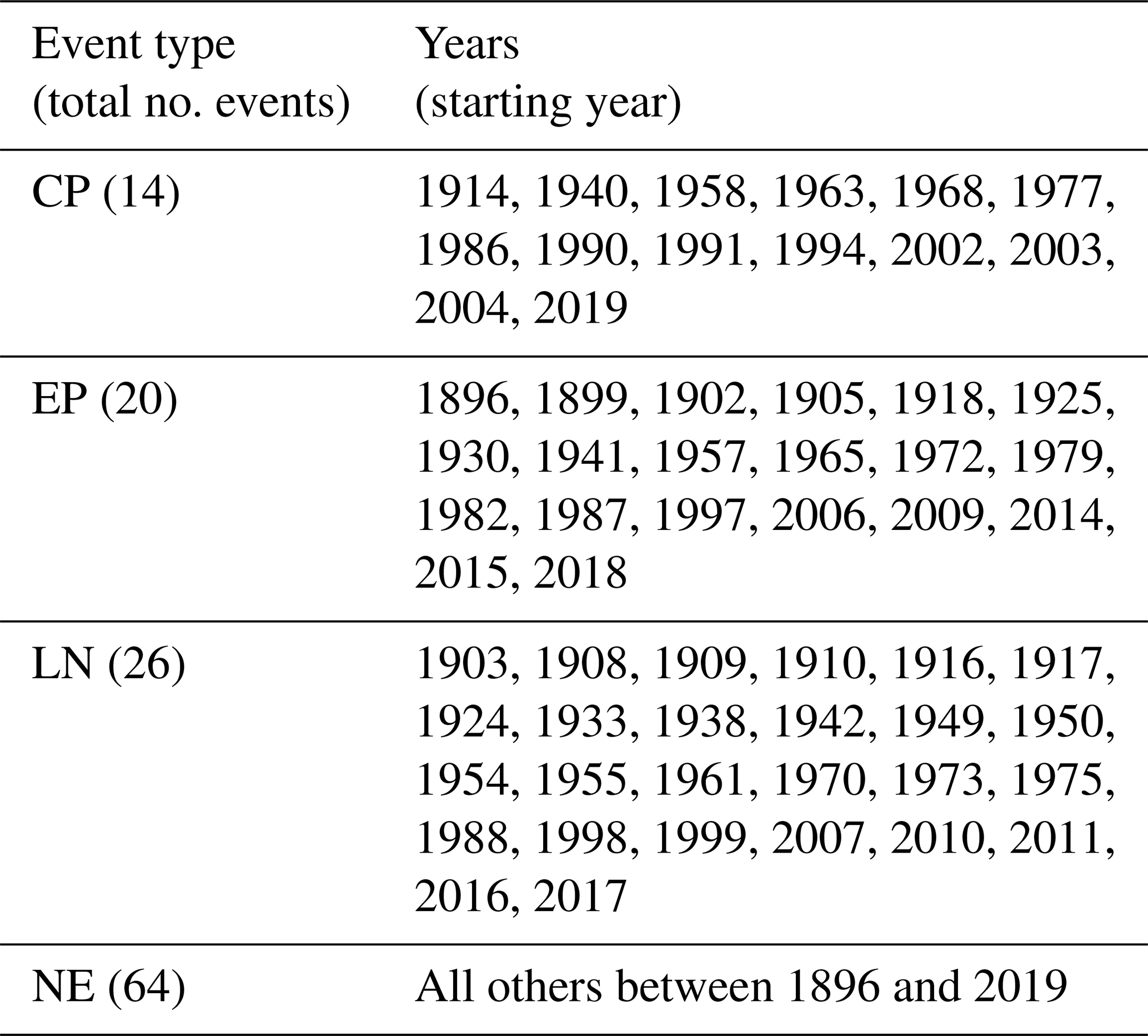
Machine learning classifiers work best with large amounts of training and testing data. Unfortunately, although for an observed climate variable SST has a relatively long record, there are only 124 years of data, which include only 14 CP events and 20 EP events (Table 1). This is an inherent problem when using climate data that has been highlighted in much of the literature (e.g. Reichstein et al., 2019). As the data are time-dependent we cannot easily acquire more data. Due to the spatial correlations within the dataset, typical machine learning augmentation methods, which would be used to artificially create additional data, are not appropriate. Instead in this study we use an unconventional augmentation method where we opt to use 18 observational and re-analysis products (Table S1 in the Supplement). Each product includes the same events with the same labels; however, due to observational uncertainty, infilling methods, and the use of re-analysis models, the SST patterns are different (e.g. Deser et al., 2010; Pascolini-Campbell et al., 2015; Huang et al., 2018). This unconventional data augmentation takes into account observational uncertainty in addition to effectively augmenting the data we have to use in this study. Before training the classifier we create anomalies by detrending the data (using a second-order polynomial) and removing the seasonal cycle (mean of each month over the entire time series after detrending).
The next step in the data preparation process is to identify which features to use in the study. While La Niña, neutral, and El Niño events are fairly easy to define, separating El Niño events into CP and EP classes can be difficult. Previous studies have identified that the Pacific SST in the predefined niño boxes, the north subtropical Pacific, and the evolution of SST over the event are the most important features for separating the two types of El Niño (e.g. Rasmusson and Carpenter, 1982; Yu and Fang, 2018; Tseng et al., 2022). In this study we use the regions niño3E (5∘ S–5∘ N, 120–90∘ W), niño3W (5∘ S–5∘ N, 120–150∘ W), niño4E (5∘ S–5∘ N, 150–170∘ W), niño4W (5∘ S–5∘ N, 170–200∘ W), and niño1.2 (0–10∘ N, 80–90∘ W) in each month from June to March as individual features to train the classifier (i.e. 5 regions × 10 months = 50 features). We note that we tested multiple feature sets including varying regions in the tropical and north subtropical Pacific and different sets of months for performance (see Sect. S2 in the Supplement), and chose this set because of its high performance in the evaluation phase.
In machine learning, part of the dataset is used for training, while the rest of the data are kept aside for evaluation of the classifier performance. In the following section, when evaluating how the classifier performs we keep the HadISST observational dataset aside and use all other data in the training phase. This choice was made due to the limited number of events in the observed record, where splitting the data by event rather than by dataset may result in the loss of events that are important to the training phase of the classification algorithm.
2.2 Choosing, training, evaluating, and tuning the classifier
Steps 3, 4, 5 and 6 – choosing, training, evaluating, and tuning the classifier – are outlined in this section. We outline these steps together as we iterate through the different steps to find the best-performing classifier. A suite of algorithms are typically used in supervised learning classifiers. It is common practice to test all algorithms and see how they perform on a particular dataset, given they all have different strengths and weaknesses. The nine algorithms tested in this study are: (1) nearest neighbours, (2) linear support vector machine, (3) radical basis function support vector machine, (4) decision tree, (5) neural network, (6) adaboost, (7) naive Bayesian, (8) quadratic discriminant analysis, and (9) random forest. We use the Python scikit-learn package (Pedregosa et al., 2011) to train each of these algorithms on our SST dataset. To evaluate each algorithm's performance, we use four different scores.
The first is an accuracy score, which defines the number of correct predictions out of all predictions:
where TP are true positives, TN are true negatives, FP are false positives, and FN are false negatives.
The second is a precision score for each of the event types (i) that we want to classify, which tells us the proportion of positive predictions that are correctly predicted:
The third is a recall score for each of the event types (i) that we want to classify, which tells us the ability to correctly predict events compared to all positive predictions for that event:
In all cases a score of 1 is best, while a score of 0 is worst. Accuracy, precision, and recall scores are calculated on the evaluation dataset.
The fourth score is an accuracy cross-validation score (CVS), which we use to test how robust our estimate is. Here, to test the classifier, the algorithm breaks the training data into n smaller datasets (in this study we use n=5). For n=5 the algorithm retrains the classifier using four of the five smaller datasets and tests on the fifth. We then obtain five accuracy scores which are averaged to give an estimate of the model performance. The CVS function in scikit-learn uses a KFold stratification to split the data into these smaller datasets (Pedregosa et al., 2011). This is designed to keep the distribution of classes similar in each set and keep sets the same size.
In this study we are particularly interested in correctly identifying CP and EP events. This means that our algorithm must have high precision and recall scores for these two events. Based on the scores outlined above, we evaluate all nine algorithms as well as ensemble classifiers that use multiple algorithms (see Sect. S2 and Table 2). The best-performing algorithm is an ensemble voting classifier, which utilises the strengths of three algorithms. These three algorithms are: a neural network, a random forest, and a nearest neighbour. The hyper-parameters of all three algorithms are tuned for optimal performance (step 6) by evaluating the performance of the algorithm using the four scores listed above at varying values of each parameter. The three algorithms chosen, the hyper-parameters used after tuning, and the scores after tuning are shown in Table 2. The ensemble voting classifier uses the wisdom of the crowd, where all three algorithms vote to give the final outcome. We choose to use soft voting as it performs better in the evaluation stage (see Sect. S2). Soft voting predicts the class label based on the maximum of the sums of the predicted probabilities. Evaluation scores for the final classifier are found in Table 2. The slightly higher scores of this final classifier compared to each individual algorithm demonstrates the utility of combining three algorithms into a ensemble voting classifier. This final classifier correctly identifies 12/13 CP (note the 2019 CP event is not included in the test set), 20/20 EP, 22/26 LN, and 64/64 NE events. Those not classified correctly are identified as NE.
Table 2Scores for different algorithms tested. Scores are defined in Sect. 2.2. Details on the tuning of the hyper-parameters can be found at https://github.com/nicolamaher/classification (last access: 22 August 2022).

Before using this classifier in step 7 to classify climate model output, we perform one more set of tests based on the following limitation. A limitation of the original evaluation is the choice of training and evaluation sets. In our original choice, where we reserve HadISST for evaluation, the same ENSO events are effectively included in both the training and evaluation sets. While this is the typical way to split the data when using data augmentation techniques, we additionally test the sensitivity to this choice. To do this we use the longer datasets (ERSSTv3b, ERSSTv4, ERSSTv5, HadISST, Kaplan, and COBE), which all cover the years 1896–2016 and separate the data so that each event is only included in the training or evaluation set.
To decide on how to separate the data into training and evaluation sets, we use the Python function train test split (Pedregosa et al., 2011), which shuffles the data then splits them into training and evaluation sets while preserving the percentages of events in both the training and testing data. We do this 10 separate times to get 10 sets of training and evaluation data and then compute the scores shown in Table 3. We additionally complete this split 100 times and manually choose 10 data splits that take CP and EP (the classes with the lowest numbers of events) from across the time series. This is done to ensure that not all events in the split come from the same part of the observational record. Since the observational data quality for SST is dependent on where in the record it occurs (e.g. lower quality early in the record), it is only appropriate to use data splits that include events across the entire record. We additionally test the algorithms with this split for HadISST alone to test the robustness of the result to using a single dataset.
Table 3Scores for the final ensemble classifier. Test 1 uses all available data, with HadISST kept aside for testing. Test 2 uses the longer datasets, ERSST, COBE, Kaplan, and HadISST, for training and testing. The data are split so that the augmented events must all occur in the same section of the data (i.e. training or testing). The data split is randomly completed 10 times on alternative splits of the training and testing data. To complete this we use the Python function train test split. Test2 w/check again uses the same function, but 10 data splits are manually chosen to ensure that they sample events from across the time dimension and have a reasonable amount of each type of event. Test2 w/check HadISST uses the same splits as Test2 w/check, but only uses HadISST for training and testing.
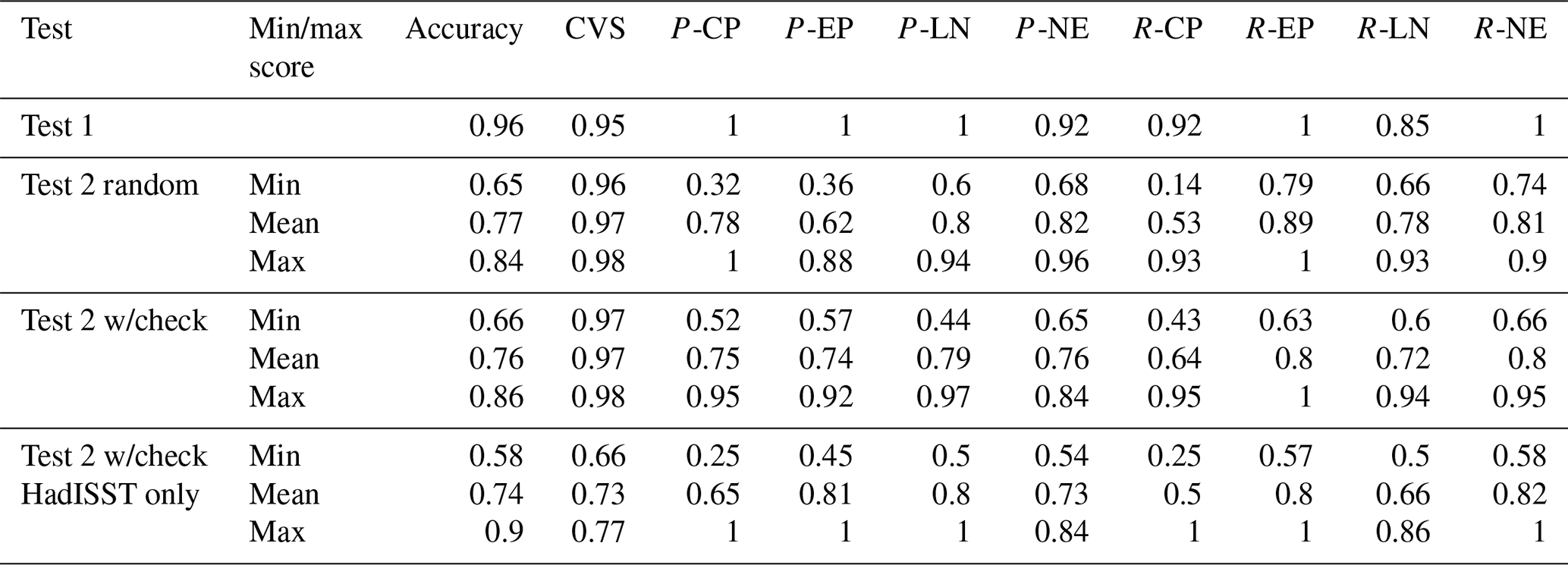
We find that for all three data splits, there is a range of accuracy that depends on how the training and evaluation sets are constructed. We find that while the precision and recall scores can be quite low for some training and evaluation sets, other sets show high precision and recall, suggesting that the algorithm can perform reasonably well. This suggests that if the training and evaluation sets are constructed in an ineffective way and the training set does not include specific events vital for classification, then the testing result is poor. This is a problem that occurs due to our small data size. Based on these results when training the final classifier, we choose to use all available data (including HadISST) so as not to lose information by excluding events. This final classifier is used in step 7 (prediction) to identify each type of ENSO event in the climate model output.
2.3 Prediction
In machine learning, step 7 – prediction – refers to applying the trained classifier to other datasets. We apply the classifier trained on observed SST data to climate model output from seven SMILEs. Besides having a large number of events to classify, the advantage of using SMILEs is that we can assess how internal climate variability can affect what we observe in our single realisation of the world. In this study we use five SMILEs with CMIP5 forcing (historical and RCP8.5) and two SMILEs with CMIP6 forcing (historical and SSP370), all of which have more than 20 members (Table S2). We classify using the same features as in our training and evaluation data. We note that if large forced changes in the SST in the tropical Pacific occur under the future scenario, the algorithm will have difficulty classifying future states as it is constrained by the information provided in the observational record. We assess changes in the SST and precipitation patterns, amplitude, and frequency of each event type. Amplitude is calculated as the November, December, January mean for the region 160∘ E to 80∘ W between 5∘ N and 5∘ S after the ensemble mean has been removed for each event in a single ensemble member, taken as a running calculation along the time series for 30-year periods. Frequency is calculated as the number of events in a single ensemble member per 30 years, taken as a running calculation along the time series. We discuss the SMILE classification results in the following sections.
3.1 Can SMILEs capture the observed CP and EP El Niño events and La Niña events?
We find CP and EP El Niño events as well as La Niña events in all models, and we identify known biases in their spatial patterns (Fig. 1). The composite spatial patterns of SST in the peak ENSO season (November, December, January) for each different ENSO class in comparison with the HadISST composites are shown in Fig. 1. CP events are visibly weaker than EP events in both the SMILEs and observations. The known bias of ENSO where SST anomalies extend too far to the west is also clearly visible in all SMILEs, although it is more prominent in some models than others. The CSIRO model shows particularly strong SST biases, with a peak SST anomaly too far into the western Pacific.
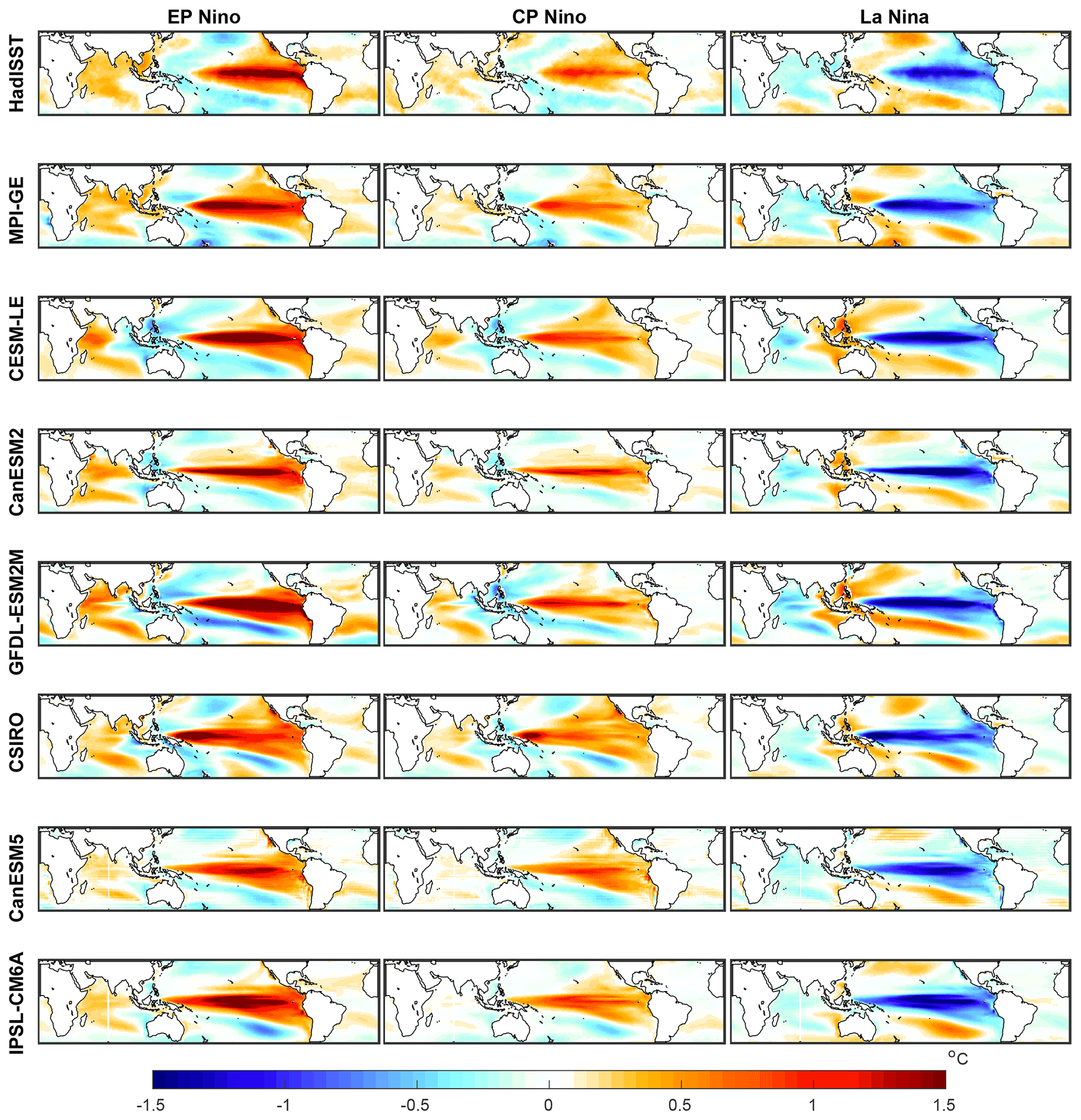
Figure 1SST pattern for composites of EP and CP El Niño events and La Niña events (left, middle, and right columns respectively); shown for HadISST observations (top row) and each individual SMILE (in order of appearance: MPI-GE, CESM-LE, CanESM2, GFDL-ESM2M, CSIRO, CanESM5, and IPSL-CM6A). The SST pattern is shown for the November, December, January average. SMILE data have the forced response (ensemble mean) removed prior to calculation, HadISST is detrended using a second-order polynomial, and then each month's average is removed. The time period used is all of the historical period, which is shown for the observations in Table S1 and SMILEs in Table S2.
The time-evolution of the SST anomalies is found to be different for each event type and appears to be important for classification (Fig. 2). We find that the machine learning classifier does not only learn the SST pattern shown in Fig. 1 and that CP events are weaker than EP events. It also correctly identifies the general pattern of how the SST anomalies evolve over the event, with CP El Niño events initiated in the central Pacific, while EP El Niño events begin in the eastern Pacific off the South American coastline and evolve into the central Pacific over the course of the event. This is supported by the fact that the classifier performs better when information about the time-evolution is included in the feature choice (see Sects. 2.1 and S2.1). The two CMIP6 models have smaller relative SST anomalies than observations, with the relative SST anomalies in the CMIP5 models more realistic in magnitude (assuming that the observed record is long enough to sample these events). Overall, all models bar CSIRO show both a realistic evolution of both EP and CP events as well as the differences between the two.

Figure 2Hovmöller diagram of relative SST along the Equator in the Pacific Ocean for composites of EP and CP El Niño events and EP minus CP El Niño events (top, middle, and bottom row respectively); shown for HadISST observations (left column) and each individual SMILE (in order of appearance: MPI-GE, CESM-LE, CanESM2, GFDL-ESM2M, CSIRO, CanESM5, and IPSL-CM6A). SST is averaged between 5N and 5S and shown for August to April. SMILE data have the forced response (ensemble mean) removed before calculation, HadISST is detrended using a second-order polynomial, and then each month's average is removed. The time period used is all of the historical period, which is shown for the observations in Table S1 and SMILEs in Table S2. Relative SST is calculated by removing the average SST between 120 and 280∘ E individually for each month.
Due to the relatively short observational record, which has been shown to be insufficient to capture multi-decadal ENSO variability (Wittenberg, 2009; Maher et al., 2018; Milinski et al., 2020), we compare the range of frequencies found across each ensemble with observations (Table 4). We find that the observed frequencies of EP and CP El Niño events and La Niña events are within the SMILE spread for most models. Individually, CanESM5 does not realistically capture EP or CP El Niño frequency, CSIRO has too low frequency of CP El Niño and La Niña events, and IPSL-CM6A has too low frequency of CP El Niño events. We also consider the pattern correlation between EP and CP events as compared to the observed pattern correlation to see how similar EP and CP Niño events can look due to internal variability (Table 4). We find that the observed pattern correlation is always captured within the ensemble range of all SMILEs. However, individual ensemble members can have a large range of pattern correlations. This demonstrates that when using single realisations, a model may appear to not represent well the distinct EP and CP patterns by chance rather than due to model deficiencies.
Table 4Frequency of events (as a percentage) in the historical period for observations (HadISST) and the SMILEs, as well as the correlation between EP and CP patterns. The mean frequency and correlation across each ensemble is shown with the minimum and maximum values in brackets. The time period used is all of the historical period, which is shown for the observations in Table S1 and SMILEs in Table S2.
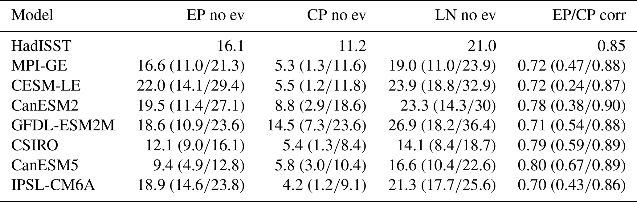
Given climate models have known ENSO biases, particularly in the location of SST anomalies along the Equator, we additionally classify by shifting the longitudes of the niño regions. This shift is defined as the difference in location between the maximum variability between 5∘ N and 5∘ S in the Pacific Ocean in the observations and the maximum variability in each individual SMILE (Table S5). We find that this does not significantly change the results in the previous paragraphs except for CSIRO frequency where EP Niño events and La Niña events are now more realistically represented. This method additionally does not change the results for climate projections presented in the following sections (see Sect. S3).
When comparing these results with previous work, different studies identify different models as more realistic or able to represent different ENSO event types (e.g. Xu et al., 2017; Capotondi et al., 2020; Feng et al., 2020; Dieppois et al., 2021). From our comparison with observations, we have assessed that most models capture the observed frequency of all event types and the correlation between the EP and CP Niño patterns, and demonstrate that previous work could find a variety of results for the same models due to the use of single realisations. We show that all models exhibit some SST bias, but that EP and CP events are differentiated in the models for physically interpretable reasons. In this case the classifier identifies the spatial pattern, evolution, and amplitude of the different event types. However, just because some observed quantities fall within the SMILE range, does not mean each model does not have individual and differing biases in other quantities, as presented by Bellenger et al. (2014); Karamperidou et al. (2017); Kohyama et al. (2017); Cai et al. (2018, 2021); Planton et al. (2021). ENSO complexity itself includes not only diversity in the form of EP and CP El Niño events, but other metrics such as the transition, propagation, and duration of events (e.g. Chen et al., 2017a; Timmermann et al., 2018; Fang and Yu, 2020). While the propagation of events is to some extent accounted for in the classifier with inclusion of the evolution over time, other metrics of ENSO complexity are also important in understanding ENSO events and could be considered using SMILEs in future work. Given the validation performed in this section, we choose to include all models except CSIRO in the following analysis of projections. This is because CSIRO presents consistent strong biases in the pattern, evolution, and frequency of events.
3.2 Can the observed increase in frequency of CP El Niño events be explained by internal variability, and what does this imply for future projections?
The frequency of CP events was observed to increase after the 1970s (An and Wang, 2000) leading to the question of whether this was a forced change due to increasing greenhouse gas emissions (Yeh et al., 2009). In Fig. 3 we show that the range of frequencies in CP (and EP and La Niña) events across an individual SMILE for a 30-year period is large. This implies that the observed increase in CP events could be due to internal variability alone, similar to Pascolini-Campbell et al. (2015) and Dieppois et al. (2021), who pointed out that CP frequency varies on multi-decadal timescales. This is the case in the SMILEs, when we consider a single ensemble member (Fig. 3; green lines) there are periods where it sits higher and lower in the ensemble spread, demonstrating this multi-decadal variability. However, when we consider trends in individual ensemble members we get a different result. Observations show an increasing trend in frequency (defined as the number of events per 30 years) of year for the entire observed period (1896–2019). The two models that cover the whole period do not capture this trend (max trend MPI-GE = 5.0, CanESM5 = 5.0). When we consider the shorter, better observed time period of 1950 onwards, the trend in observations increases to 8.4. However, in this case all models that cover the entire time period are able to capture this trend (max trend MPI-GE = 15.1, CESM-LE = 13.3, CanESM2 = 11.3, GFDL-ESM2M = 19.7, CanESM5 = 11.9). This suggests that the observed increase in CP could be due to internal variability alone, as the models capture the increase in CP events in the better observed period; however, the inconsistencies in the earlier period also highlight potential model biases.
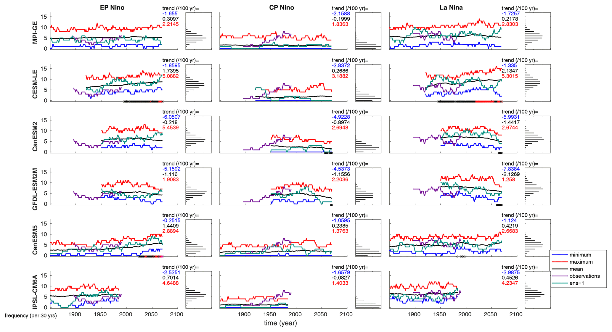
Figure 3ENSO frequency in each SMILE for EP and CP El Niño events and for La Niña events (left, middle, and right columns respectively). Black line shows the ensemble mean for each year, red line shows the ensemble maximum, blue line shows the ensemble minimum, purple line represents HadISST observations, and green line is the first ensemble member. Frequency is calculated as the number of events in a single ensemble member per 30 years, taken as a running calculation along the time series. PDFs show the distribution of ensemble members for the entire time series. Black dots on the x axis demonstrate when the signal (current ensemble mean minus the ensemble mean at the beginning of the time series) is greater than the noise (standard deviation taken across the ensemble). Red dots show when the signal is 1.645 times the noise, while magenta dots show the same when the signal is greater than 2 times the noise. These thresholds correspond to the likely, very likely, and extremely likely ranges. Maximum (red), mean (black), and minimum (blue) trends across the individual ensemble members are shown in text at the top right of each panel. We note that the trends are calculated over the entirety of the simulation length for each SMILE. This means that due to the different time periods covered, trends are not directly comparable between different SMILEs.
When assessing projected changes in frequency, we use a signal-to-noise ratio to identify changes. When the signal at any time point (ensemble mean at the time point minus the ensemble mean at the beginning of the time-series) is greater than the noise (standard deviation taken across the ensemble) we identify a likely projected change. When the signal is 1.645 or 2 times the noise these thresholds correspond to the very likely and extremely likely. CESM-LE and CanESM5 show very likely and extremely likely increases in EP El Niño frequency respectively (Fig. 3). CESM-LE projects a very likely increase in La Niña frequency with small likely decreases found at the end of the century for CanESM2 and GFDL-ESM2M. No model projects a significant change in CP frequency before the end of the century, where CanESM2 and GFDL-ESM2M project a likely decrease in frequency. We note that large changes could be observed due to the considerable internal variability of these frequencies alone as demonstrated by the maximum and minimum frequencies, range of maximum and minimum trends across ensemble members, and the multi-decadal changes seen in the individual ensemble members (e.g. green line in Fig. 3). These results are interesting in the context of a palaeoclimate study by Freund et al. (2019), who show that the current relative frequency of EP CP events is unprecedented in the palaeoclimate record. There are two possible reasons for the differences between this study and our results. First, model biases may mean that the models cannot capture this shift correctly. Second, a shift in frequencies may have already occurred, after which we do not project further future shifts. This could be investigated further in future studies by applying this classification method to the last millennium-long palaeoclimate model simulations.
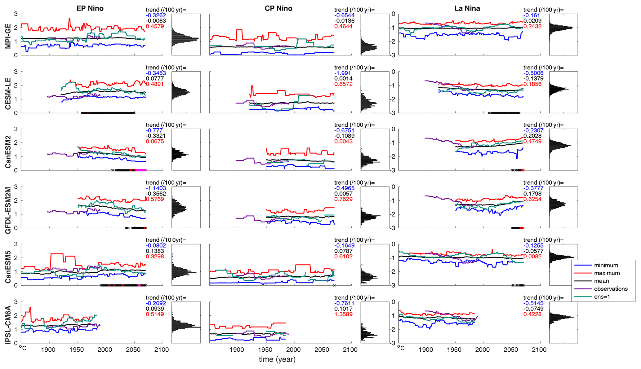
Figure 4ENSO amplitude in each SMILE for EP and CP El Niño events and for La Niña events (left, middle ,and right columns respectively). Black line shows the ensemble mean for each year, red line shows the ensemble maximum, blue line shows the ensemble minimum, purple line represents HadISST observations, and green line is the first ensemble member. Amplitude is calculated as the November, December, January mean for the region 160∘ E to 80∘ W between 5∘ N and 5∘ S after the ensemble mean has been removed for each event in a single ensemble member, taken as a running calculation along the time series for 30-year periods. PDFs show the distribution of ensemble members for the entire time series. Black dots on the x axis demonstrate when the signal (current ensemble mean minus the ensemble mean at the beginning of the time series) is greater than the noise (standard deviation taken across the ensemble). Red dots show when the signal is 1.645 times the noise, while magenta dots show the same when the signal is greater than 2 times the noise. These thresholds correspond to the likely, very likely, and extremely likely ranges. Maximum (red), mean (black), and minimum (blue) trends across the individual ensemble members are shown in text at the top right of each panel. We note that the trends are calculated over the entirety of the simulation length for each SMILE. This means that due to the different time periods covered, trends are not directly comparable between different SMILEs.
3.3 Do we project changes in the amplitude, SST, and precipitation patterns of each event type?
When considering ENSO amplitude (November, December, January mean for the region 160∘ E to 80∘ W between 5∘ N and 5∘ S after the ensemble mean has been removed for each event), similar to frequency we find that the range of amplitudes across each SMILE at any given time is quite large (0.5–1.5 ∘C) for each event type, with the difference between the maximum and minimum trends ranging from 0.1–2.5 ∘C per 100 years across models (Fig. 4). This agrees well with previous work that shows that ENSO amplitude is very variable in single realisations of climate models (e.g. Wittenberg, 2009; Maher et al., 2018; Ng et al., 2021; Dieppois et al., 2021). When projecting future changes, we find model disagreement on the forced change in EP El Niño and La Niña amplitude (Fig. 4). We find model agreement of no change in CP El Niño amplitude. We find a likely increase in the amplitude of EP events in CESM-LE and CanESM5, with likely and extremely likely decreases in GFDL-ESM2M and CanESM2 respectively. For La Niña events there is a likely decrease in CESM-LE and CanESM5, and very likely increases in CanESM2 and GFDL-ESM2M.
These results compare well to previous work, where El Niño amplitude was found to increase in CESM-LE, not change in MPI-GE, and decrease in GFDL-ESM2M (Zheng et al., 2017; Haszpra et al., 2020; Maher et al., 2018, 2021; Ng et al., 2021). When partitioning amplitude changes into EP and CP events using different criteria for classification, Ng et al. (2021) found an increase in both EP and CP amplitude in CESM-LE and no change in MPI-GE. This agrees well with our results, although we do not see the increase in CP amplitude in CESM-LE, possibly due to the different time periods used and the relatively small magnitude of the change. Recently Cai et al. (2018) and Cai et al. (2021) showed that for CMIP5 and CMIP6 models that represent some ENSO properties well, EP amplitude increases in most models. However, only two of the models they identified as able to represent ENSO well are included in our study (CESM-LE and GFDL-ESM2M) and they differ in sign (increasing amplitude in CESM-LE; decreasing amplitude in GFDL-ESM2M). This is in agreement with Cai et al. (2018), who also found decreasing amplitude in GFDL-ESM2M, which was an outlier in their study that used single ensemble members from CMIP5.
These model differences have been suggested to be related to changes in the zonal gradient of mean SST. Wang et al. (2019) suggest that an increase in the SST gradient results in an increase in the amplitude of strong basin-wide El Niño events, with a decrease leading to a decrease in amplitude. Kohyama et al. (2017), however, suggest that a La Niña-like warming pattern (i.e. the western Pacific warms more than the eastern Pacific, resulting in an increased zonal SST gradient) should result in a decrease in ENSO amplitude, as does Fredriksen et al. (2020). This result is in agreement with an observed decrease in tropical Pacific variability coupled with an increase in the trade winds and increase in thermocline tilt from 2000 to 2011 as compared to 1979–1999 (Hu et al., 2013). Beobide-Arsuaga et al. (2021) also find a weak negative correlation between the two quantities in CMIP5 and CMIP6 models. In our study, two of the five SMILEs additionally show a weak negative relationship between these quantities (MPI-GE and GFDL-ESM2M); however, three models (CESM-LE, CanESM2, and CanESM5) show no relationship (Fig. S2a in the Supplement). We find no relationship between CP amplitude and the projected change in the zonal mean SST gradient (Fig. S2b), consistent with Fredriksen et al. (2020).
We next plot the change in SST pattern for each event type for the period 2050–2099 as compared to 1950–1999 (Fig. 5). We use detrended data to look at the changes in ENSO itself, outside of mean state changes. We find similar pattern changes for EP and CP events, with the opposite change for La Niña events. The SST pattern change lacks agreement across the models. Potentially this is related to the mean state changes (Knutson et al., 1997; McPhaden et al., 2011; Hu et al., 2013; Kim et al., 2014; Kohyama et al., 2017; Wang et al., 2019; Beobide-Arsuaga et al., 2021); however, the SST pattern change is different for CESM-LE and CanESM2, which have similar mean state changes suggesting that the relationship is more complicated than one simple metric.

Figure 5Change in SST pattern in each SMILE in the period 2050–2099 as compared to 1950–1999 for EP and CP El Niño events and for La Niña events (left, centre left, and centre right columns respectively. The mean state change in SST is shown in the right column; shown for each individual SMILE (in order of appearance: MPI-GE, CESM-LE, CanESM2, GFDL-ESM2M, CanESM5) and the multi-ensemble mean (bottom row). The SST pattern is calculated as the November, December, January average and composited for each event type over each time period. The relative mean state change is calculated as the ensemble mean SST over each time period, with the earlier period subtracted from the latter relative to the total change in the region shown (0–360∘ E, 40∘ S–40∘ N). SMILE data have the forced response (ensemble mean) removed prior to calculation for the SST change, but not the mean state change.
Precipitation projections for each event type also show large differences between SMILEs (Fig. 6). These projected pattern differences are, however, found to be linked to the projected SST patterns, with contours of increasing SST found to closely correspond to wetting, and decreasing SST to drying. This clarifies that ENSO changes in SST and precipitation are linked and that it is not possible to truly understand one without the other.
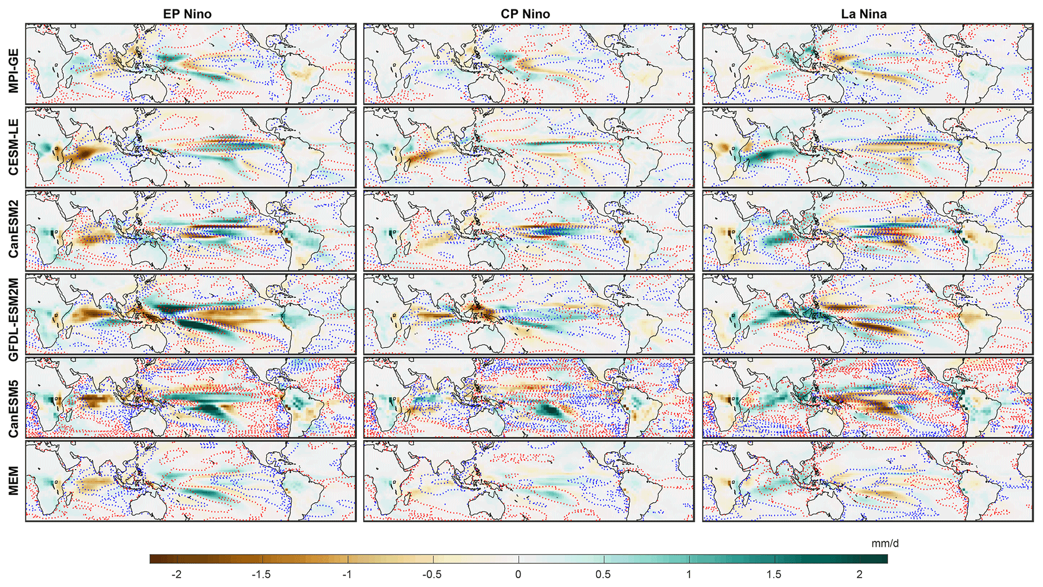
Figure 6Change in precipitation pattern in each SMILE in the period 2050–2099 as compared to 1950–1999 for EP and CP El Niño events and for La Niña events (left, middle, and right columns respectively). The SST change from Fig. 5 is shown as contours for reference (blue for cooling, red for warming); shown for each individual SMILE (in order of appearance: MPI-GE, CESM-LE, CanESM2, GFDL-ESM2M, CanESM5) and the multi-ensemble mean (bottom row). The precipitation pattern is calculated as the November, December, January average and composited for each event type over each time period. SMILE data have the forced response (ensemble mean) removed prior to calculation.
We compare the multi-ensemble mean patterns (Fig. 6) with previous work using CMIP models. Xu et al. (2017) find similar strong cooling in RCP8.5 in the eastern Pacific for EP events, and some similarities of cooling in the eastern Pacific for CP events as well. For precipitation projections, EP events look similar to Xu et al. (2017) and show a general increase in precipitation, particularly in the central Pacific; however, CP events look quite different. This is most likely due to the definitions used by Xu et al. (2017) where they define EP events as the first empirical orthogonal function (EOF1) in tropical Pacific, and CP as the second empirical orthogonal function (EOF2). Other studies have, however, suggested that it is the combination of EOF1 and EOF2 that should be used to identify EP and CP events (Takahashi et al., 2011). When comparing CMIP5 projections from Power et al. (2013), who also look at EOF1, some similarities are found for precipitation projections, but SST projections look quite different. These results probably differ both due to different definitions of event types as well as the different set of models used and differences between single model realisations and SMILEs. We note that we also consider extreme El Niño events, and discuss results for this event type in Sect. S4.
In this study we use supervised machine learning combined with observed SST products to develop a new classifier for ENSO events, which classifies events into La Niña, neutral, eastern Pacific (EP) El Niño, and central Pacific (CP) El Niño. This method uses differences in the pattern, amplitude, and evolution of events to make the classification. Using supervised machine learning has the advantage that it includes spatial and temporal information from 18 SST products to classify events without relying on pre-defined metrics, individual parameters, or manual identification. We then apply this classifier to seven SMILEs to identify ENSO events similar to those observed. By using SMILEs we examine forced changes in ENSO compared to the magnitude of internal variability. We find that
-
All SMILEs bar CSIRO capture the observed pattern, evolution, frequency, and pattern correlation of EP and CP events, although known biases in the spatial pattern (e.g. SST anomalies located too far west) are found.
-
The observed increase in the frequency of CP events is within the range of the SMILEs internal variability for the period 1950 onwards, but not for the entire observed record.
-
CP El Niño frequency and amplitude are not projected to change in the future. EP El Niño frequency is projected to either increase or not change.
-
The SMILEs do not agree on projections of EP El Niño amplitude and La Niña frequency and amplitude. EP event amplitude projections are found to be weakly linked to changes in the zonal-mean gradient across the Pacific in two out of five models.
-
Models show differences in projected patterns of ENSO SST and precipitation that do not seem to be simply linked to the tropical Pacific mean state changes. However, the precipitation and SST changes in individual models are linked.
In conclusion, supervised machine learning has been used to build a new ENSO classifier for climate models that takes into account SST evolution along the tropical Pacific, and can be used to identify events that behave similarly to those observed. Future work running all classification schemes on SMILEs and comparing this new supervised learning algorithm with other methods would be informative for comparisons of the use of different classification schemes. We find that the models do not project changes in CP El Niño frequency or amplitude, project either no change or an increase in EP El Niño frequency, and demonstrate disparity in future changes in other event types and in the projected spatial patterns of SST and precipitation. The large ensemble spread for frequency and amplitude highlights, similar to previous work, that SMILEs are needed to evaluate ENSO and make projections due to the large variability of ENSO characteristics on decadal and longer timescales.
The data that support the findings of this study are openly available at the following locations: MPI-GE, https://esgf-data.dkrz.de/projects/mpi-ge/ (Max-Planck-Institut für Meteorologie, 2022), all other CMIP5 large ensembles (CanESM2, CESM-LE, CSIRO-Mk3-6-0, GFDL-ESM2M); https://www.cesm.ucar.edu/projects/community-projects/MMLEA/ (NCAR/UCAR, 2022) and CMIP6, https://esgf-data.dkrz.de/projects/cmip6-dkrz/ (World Climate Research Programme, 2022). Source code for the machine learning classifier and the observed data which it is trained on can be found on github at: https://github.com/nicolamaher/classification (last access: 29 August 2022, https://doi.org/10.5281/zenodo.7032576, Maher, 2022a). Derived data and post-processing scripts supporting the findings of this study are available from https://pure.mpg.de/ (Maher, 2022b). References for the data used in this study can be found for observations and re-analysis products in Table S1 and SMILEs in Table S2. COBE, GODAS, KAPLAN, and OISST data were provided by the NOAA/OAR/ESRL PSL, Boulder, Colorado, USA, from their website at https://www.psl.noaa.gov/data/gridded/ (NOAA Physical Sciences Laboratory, 2022).
The supplement related to this article is available online at: https://doi.org/10.5194/esd-13-1289-2022-supplement.
NM and TPT jointly devised the study. TPT provided the machine learning expertise and NM provided the ENSO expertise. SM had the idea to use multiple SST products and re-analysis for data augmentation. NM completed the analysis and wrote the manuscript with critical input from TPT and SM.
The contact author has declared that none of the authors has any competing interests.
Publisher’s note: Copernicus Publications remains neutral with regard to jurisdictional claims in published maps and institutional affiliations.
We thank Jeff Exbrayat for his discussion on machine learning, Elizabeth Barnes for her comments on the project, including testing/training split, John O'Brien for his ideas on extreme ENSO section, and Malte Stuecker for his comments on the 2019/2020 state of the tropical Pacific. We additionally thank Goratz Beobide Arsuaga for his internal review of this manuscript and Antonietta Capotondi for her comments on the manuscript. Finally, we thank Jochem Marotzke for his mentorship and support of this project. We thank the US National Science Foundation, National Oceanic and Atmospheric Administration, National Aeronautics and Space Administration, and Department of Energy for sponsoring the activities of the US CLIVAR Working Group on Large Ensembles.
Nicola Maher was partially supported by the Max Planck Society for the Advancement of Science, in part by NSF AGS 1554659 and in part by the CIRES Visiting Fellows Program and the NOAA Cooperative Agreement with CIRES, NA17OAR4320101. Sebastian Milinski was also supported by the Max Planck Society for the Advancement of Science.
The article processing charges for this open-access publication were covered by the Max Planck Society.
This paper was edited by Yun Liu and reviewed by two anonymous referees.
An, S.-I. and Wang, B.: Interdecadal Change of the Structure of the ENSO Mode and Its Impact on the ENSO Frequency, J. Climate, 13, 2044–2055, https://doi.org/10.1175/1520-0442(2000)013<2044:ICOTSO>2.0.CO;2, 2000. a, b
Ashok, K., Behera, S. K., Rao, S. A., Weng, H., and Yamagata, T.: El Niño Modoki and its possible teleconnection, J. Geophys. Res.-Oceans, 112, C11007, https://doi.org/10.1029/2006JC003798, 2007. a
Barnes, E. A., Hurrell, J. W., Ebert-Uphoff, I., Anderson, C., and Anderson, D.: Viewing Forced Climate Patterns Through an AI Lens, Geophys. Res. Lett., 46, 13389–13398, https://doi.org/10.1029/2019GL084944, 2019. a
Barnes, E. A., Toms, B., Hurrell, J. W., Ebert-Uphoff, I., Anderson, C., and Anderson, D.: Indicator Patterns of Forced Change Learned by an Artificial Neural Network, J. Adv. Model. Earth Sy., 12, e2020MS002195, https://doi.org/10.1029/2020MS002195, 2020. a
Bellenger, H., Guilyardi, E., Leloup, J., Lengaigne, M., and Vialard, J.: ENSO representation in climate models: from CMIP3 to CMIP5, Clim. Dynam., 42, 1999–2018, https://doi.org/10.1007/s00382-013-1783-z, 2014. a
Beobide-Arsuaga, G., Bayr, T., Reintges, A., and Latif, M.: Uncertainty of ENSO-amplitude projections in CMIP5 and CMIP6 models, Clim. Dynam., 56, 3875–3888, https://doi.org/10.1007/s00382-021-05673-4, 2021. a, b
Cai, W., Borlace, S., Lengaigne, M., van Rensch, P., Collins, M., Vecchi, G., Timmermann, A., Santoso, A., McPhaden, M. J., Wu, L., England, M. H., Wang, G., Guilyardi, E., and Jin, F.-F.: Increasing frequency of extreme El Niño events due to greenhouse warming, Nat. Clim. Change, 4, 111–116, https://doi.org/10.1038/nclimate2100, 2014. a
Cai, W., Wang, G., Dewitte, B., Wu, L., Santoso, A., Takahashi, K., Yang, Y., Carréric, A., and McPhaden, M. J.: Increased variability of eastern Pacific El Niño under greenhouse warming, Nature, 564, 201–206, https://doi.org/10.1038/s41586-018-0776-9, 2018. a, b, c, d
Cai, W., Santoso, A., Collins, M., Dewitte, B., Karamperidou, C., Kug, J.-S., Lengaigne, M., McPhaden, M. J., Stuecker, M. F., Taschetto, A. S., Timmermann, A., Wu, L., Yeh, S.-W., Wang, G., Ng, B., Jia, F., Yang, Y., Ying, J., Zheng, X.-T., Bayr, T., Brown, J. R., Capotondi, A., Cobb, K. M., Gan, B., Geng, T., Ham, Y.-G., Jin, F.-F., Jo, H.-S., Li, X., Lin, X., McGregor, S., Park, J.-H., Stein, K., Yang, K., Zhang, L., and Zhong, W.: Changing El Niño-Southern Oscillation in a warming climate, Nature Reviews Earth & Environment, 2, 628–644, https://doi.org/10.1038/s43017-021-00199-z, 2021. a, b, c
Capotondi, A., Wittenberg, A. T., Newman, M., Lorenzo, E. D., Yu, J.-Y., Braconnot, P., Cole, J., Dewitte, B., Giese, B., Guilyardi, E., Jin, F.-F., Karnauskas, K., Kirtman, B., Lee, T., Schneider, N., Xue, Y., and Yeh, S.-W.: Understanding ENSO Diversity, B. Am. Meteorol. Soc., 96, 921–938, https://doi.org/10.1175/BAMS-D-13-00117.1, 2015. a, b
Capotondi, A., Wittenberg, A. T., Kug, J.-S., Takahashi, K., and McPhaden, M. J.: ENSO Diversity, in: El Niño Southern Oscillation in a Changing Climate, edited by: McPhaden, M. J., Santoso, A., and Cai, W., https://doi.org/10.1002/9781119548164.ch4, 2020. a, b, c, d
Chen, C., Cane, M. A., Wittenberg, A. T., and Chen, D.: ENSO in the CMIP5 Simulations: Life Cycles, Diversity, and Responses to Climate Change, J. Climate, 30, 775–801, https://doi.org/10.1175/JCLI-D-15-0901.1, 2017a. a
Chen, L., Li, T., Yu, Y., and Behera, S. K.: A possible explanation for the divergent projection of ENSO amplitude change under global warming, Clim. Dynam., 49, 3799–3811, https://doi.org/10.1007/s00382-017-3544-x, 2017b. a
Chung, C. T. Y., Power, S. B., Arblaster, J. M., Rashid, H. A., and Roff, G. L.: Nonlinear precipitation response to El Niño and global warming in the Indo-Pacific, Clim. Dynam., 42, 1837–1856, https://doi.org/10.1007/s00382-013-1892-8, 2014. a
Deser, C., Phillips, A. S., and Alexander, M. A.: Twentieth century tropical sea surface temperature trends revisited, Geophys. Res. Lett., 37, L10701, https://doi.org/10.1029/2010GL043321, 2010. a
Dieppois, B., Capotondi, A., Pohl, B., Chun, K. P., Monerie, P.-A., and Eden, J.: ENSO diversity shows robust decadal variations that must be captured for accurate future projections, Communications Earth & Environment, 2, 212, https://doi.org/10.1038/s43247-021-00285-6, 2021. a, b, c
Fang, S.-W. and Yu, J.-Y.: Contrasting Transition Complexity Between El Niño and La Niña: Observations and CMIP5/6 Models, Geophys. Res. Lett., 47, 2020GL088926, https://doi.org/10.1029/2020GL088926, 2020. a
Feng, J., Lian, T., Ying, J., Li, J., and Li, G.: Do CMIP5 Models Show El Niño Diversity?, J. Climate, 33, 1619–1641, https://doi.org/10.1175/JCLI-D-18-0854.1, 2020. a
Fredriksen, H.-B., Berner, J., Subramanian, A. C., and Capotondi, A.: How Does El Niño–Southern Oscillation Change Under Global Warming – A First Look at CMIP6, Geophys. Res. Lett., 47, e2020GL090640, https://doi.org/10.1029/2020GL090640, 2020. a, b
Freund, M. B., Henley, B. J., Karoly, D. J., McGregor, H. V., Abram, N. J., and Dommenget, D.: Higher frequency of Central Pacific El Niño events in recent decades relative to past centuries, Nat. Geosci., 12, 450–455, https://doi.org/10.1038/s41561-019-0353-3, 2019. a, b, c
Giese, B. S. and Ray, S.: El Niño variability in simple ocean data assimilation (SODA), 1871–2008, J. Geophys. Res.-Oceans, 116, C02024, https://doi.org/10.1029/2010JC006695, 2011. a
Gil, Y., Pierce, S. A., Babaie, H., Banerjee, A., Borne, K., Bust, G., Cheatham, M., Ebert-Uphoff, I., Gomes, C., Hill, M., Horel, J., Hsu, L., Kinter, J., Knoblock, C., Krum, D., Kumar, V., Lermusiaux, P., Liu, Y., North, C., Pankratius, V., Peters, S., Plale, B., Pope, A., Ravela, S., Restrepo, J., Ridley, A., Samet, H., Shekhar, S., Skinner, K., Smyth, P., Tikoff, B., Yarmey, L., and Zhang, J.: Intelligent Systems for Geosciences: An Essential Research Agenda, Commun. ACM, 62, 76–84, https://doi.org/10.1145/3192335, 2018. a
Guo, Y., Cao, X., Liu, B., and Peng, K.: El Niño Index Prediction Using Deep Learning with Ensemble Empirical Mode Decomposition, Symmetry, 12, 893, https://doi.org/10.3390/sym12060893, 2020. a
Ham, Y.-G., Jeong, Y., and Kug, J.-S.: Changes in Independency between Two Types of El Niño Events under a Greenhouse Warming Scenario in CMIP5 Models, J. Climate, 28, 7561–7575, https://doi.org/10.1175/JCLI-D-14-00721.1, 2015. a
Ham, Y.-G., Kim, J.-H., and Luo, J.-J.: Deep learning for multi-year ENSO forecasts, Nature, 573, 568–572, https://doi.org/10.1038/s41586-019-1559-7, 2019. a
Haszpra, T., Herein, M., and Bódai, T.: Investigating ENSO and its teleconnections under climate change in an ensemble view – a new perspective, Earth Syst. Dynam., 11, 267–280, https://doi.org/10.5194/esd-11-267-2020, 2020. a
Hendon, H. H., Lim, E., Wang, G., Alves, O., and Hudson, D.: Prospects for predicting two flavors of El Niño, Geophys. Res. Lett., 36, L19713, https://doi.org/10.1029/2009GL040100, 2009. a
Hu, Z.-Z., Kumar, A., Ren, H.-L., Wang, H., L’Heureux, M., and Jin, F.-F.: Weakened Interannual Variability in the Tropical Pacific Ocean since 2000, J. Climate, 26, 2601–2613, https://doi.org/10.1175/JCLI-D-12-00265.1, 2013. a, b
Huang, B., Angel, W., Boyer, T., Cheng, L., Chepurin, G., Freeman, E., Liu, C., and Zhang, H.-M.: Evaluating SST Analyses with Independent Ocean Profile Observations, J. Climate, 31, 5015–5030, https://doi.org/10.1175/JCLI-D-17-0824.1, 2018. a
Huang, P. and Xie, S.-P.: Mechanisms of change in ENSO-induced tropical Pacific rainfall variability in a warming climate, Nat. Geosci., 8, 922–926, https://doi.org/10.1038/ngeo2571, 2015. a
Johnson, N. C.: How Many ENSO Flavors Can We Distinguish?, J. Climate, 26, 4816–4827, https://doi.org/10.1175/JCLI-D-12-00649.1, 2013. a
Kao, H.-Y. and Yu, J.-Y.: Contrasting Eastern-Pacific and Central-Pacific Types of ENSO, J. Climate, 22, 615–632, https://doi.org/10.1175/2008JCLI2309.1, 2009. a, b, c
Karamperidou, C., Jin, F.-F., and Conroy, J. L.: The importance of ENSO nonlinearities in tropical pacific response to external forcing, Clim. Dynam., 49, 2695–2704, https://doi.org/10.1007/s00382-016-3475-y, 2017. a
Karpatne, A., Ebert-Uphoff, I., Ravela, S., Babaie, H. A., and Kumar, V.: Machine Learning for the Geosciences: Challenges and Opportunities, IEEE T. Knowl. Data En., 31, 1544–1554, https://doi.org/10.1109/TKDE.2018.2861006, 2019. a
Kim, H.-M., webster, J., and J.A., C.: Impact of Shifting Patterns of Pacific Ocean Warming on North Atlantic Tropical Cyclones, Science, 325, 77–80, https://doi.org/10.1126/science.1174062, 2009. a
Kim, S. T., Cai, W., Jin, F.-F., Santoso, A., Wu, L., Guilyardi, E., and An, S.-I.: Response of El Niño sea surface temperature variability to greenhouse warming, Nat. Clim. Change, 4, 786–790, https://doi.org/10.1038/nclimate2326, 2014. a
Knutson, T. R., Manabe, S., and Gu, D.: Simulated ENSO in a Global Coupled Ocean–Atmosphere Model: Multidecadal Amplitude Modulation and CO2 Sensitivity, J. Climate, 10, 138–161, https://doi.org/10.1175/1520-0442(1997)010<0138:SEIAGC>2.0.CO;2, 1997. a
Kohyama, T., Hartmann, D. L., and Battisti, D. S.: La Niña–like Mean-State Response to Global Warming and Potential Oceanic Roles, J. Climate, 30, 4207–4225, https://doi.org/10.1175/JCLI-D-16-0441.1, 2017. a, b, c
Kug, J.-S., Jin, F.-F., and An, S.-I.: Two Types of El Niño Events: Cold Tongue El Niño and Warm Pool El Niño, J. Climate, 22, 1499–1515, https://doi.org/10.1175/2008JCLI2624.1, 2009. a
Lemmon, D. E. and Karnauskas, K. B.: A metric for quantifying El Niño pattern diversity with implications for ENSO-mean state interaction, Clim. Dynam., 52, 7511–7523, https://doi.org/10.1007/s00382-018-4194-3, 2019. a
Liu, Y., Cobb, K. M., Song, H., Li, Q., Li, C.-Y., Nakatsuka, T., An, Z., Zhou, W., Cai, Q., Li, J., Leavitt, S. W., Sun, C., Mei, R., Shen, C.-C., Chan, M.-H., Sun, J., Yan, L., Lei, Y., Ma, Y., Li, X., Chen, D., and Linderholm, H. W.: Recent enhancement of central Pacific El Niño variability relative to last eight centuries, Nat. Commun., 8, 15386, https://doi.org/10.1038/ncomms15386, 2017. a
Maher, N.: nicolamaher/classification: ENSO ML Classification – Maher, Tabarin, Milinski 2022 (v1.1.0), Zenodo [code], https://doi.org/10.5281/zenodo.7032576, 2022a. a
Maher, N.: Combining machine learning and SMILEs to classify, better understand, and project changes in ENSO events, MPG [code], https://pure.mpg.de/, last access: 29 August 2022b. a
Maher, N., Matei, D., Milinski, S., and Marotzke, J.: ENSO Change in Climate Projections: Forced Response or Internal Variability?, Geophys. Res. Lett., 45, 11390–11398, https://doi.org/10.1029/2018GL079764, 2018. a, b, c, d, e, f
Maher, N., Power, S., and Marotzke, J.: More accurate quantification of model-to-model agreement in externally forced climatic responses over the coming century, Nat. Commun., 12, 788, https://doi.org/10.1038/s41467-020-20635-w, 2021. a
Max-Planck-Institut für Meteorologie: MPI Grand Ensemble, https://esgf-data.dkrz.de/projects/mpi-ge/, last access: 25 August 2022. a
McPhaden, M. J., Lee, T., and McClurg, D.: El Niño and its relationship to changing background conditions in the tropical Pacific Ocean, Geophys. Res. Lett., 38, L15709, https://doi.org/10.1029/2011GL048275, 2011. a, b
Milinski, S., Maher, N., and Olonscheck, D.: How large does a large ensemble need to be?, Earth Syst. Dynam., 11, 885–901, https://doi.org/10.5194/esd-11-885-2020, 2020. a, b
NCAR/UCAR: Multi-Model Large Ensemble Archive, https://www.cesm.ucar.edu/projects/community-projects/MMLEA/, last access: 25 August 2022. a
Newman, M., Shin, S.-I., and Alexander, M. A.: Natural variation in ENSO flavors, Geophys. Res. Lett., 38, L14705, https://doi.org/10.1029/2011GL047658, 2011. a
Ng, B., Cai, W., Cowan, T., and Bi, D.: Impacts of Low-Frequency Internal Climate Variability and Greenhouse Warming on El Niño–Southern Oscillation, J. Climate, 34, 2205–2218, https://doi.org/10.1175/JCLI-D-20-0232.1, 2021. a, b, c, d, e
NOAA Physical Sciences Laboratory: Gridded Climate Data, https://www.psl.noaa.gov/data/gridded/, last access: 25 August 2022. a
Pascolini-Campbell, M., Zanchettin, D., Bothe, O., Timmreck, C., Matei, D., Jungclaus, J. H., and Graf, H.-F.: Toward a record of Central Pacific El Niño events since 1880, Theor. Appl. Climatol., 119, 379–389, https://doi.org/10.1007/s00704-014-1114-2, 2015. a, b, c, d, e, f, g
Pedregosa, F., Varoquaux, G., Gramfort, A., Michel, V., Thirion, B., Grisel, O., Blondel, M., Prettenhofer, P., Weiss, R., Dubourg, V., Vanderplas, J., Passos, A., Cournapeau, D., Brucher, M., Perrot, M., and Duchesnay, E.: Scikit-learn: Machine Learning in Python, J. Mach. Learn. Res., 12, 2825–2830, 2011. a, b, c
Planton, Y. Y., Guilyardi, E., Wittenberg, A. T., Lee, J., Gleckler, P. J., Bayr, T., McGregor, S., McPhaden, M. J., Power, S., Roehrig, R., Vialard, J., and Voldoire, A.: Evaluating Climate Models with the CLIVAR 2020 ENSO Metrics Package, B. Am. Meteorol. Soc., 102, E193–E217, https://doi.org/10.1175/BAMS-D-19-0337.1, 2021. a
Power, S., Delage, F., Chung, C., Kociuba, G., and Keay, K.: Robust twenty-first-century projections of El Niño and related precipitation variability, Nature, 502, 541–545, https://doi.org/10.1038/nature12580, 2013. a, b
Rasmusson, E. M. and Carpenter, T. H.: Variations in Tropical Sea Surface Temperature and Surface Wind Fields Associated with the Southern Oscillation/El Niño, Mon. Weather Rev., 110, 354–384, https://doi.org/10.1175/1520-0493(1982)110<0354:VITSST>2.0.CO;2, 1982. a
Reichstein, M., Camps-Valls, G., Stevens, B., Jung, M., Denzler, J., Carvalhais, N., and Prabhat: Deep learning and process understanding for data-driven Earth system science, Nature, 566, 195–204, https://doi.org/10.1038/s41586-019-0912-1, 2019. a, b
Ren, H.-L. and Jin, F.-F.: Niño indices for two types of ENSO, Geophys. Res. Lett., 38, L04704, https://doi.org/10.1029/2010GL046031, 2011. a
Takahashi, K., Montecinos, A., Goubanova, K., and Dewitte, B.: ENSO regimes: Reinterpreting the canonical and Modoki El Niño, Geophys. Res. Lett., 38, L10704, https://doi.org/10.1029/2011GL047364, 2011. a, b
Timmermann, A., An, S.-I., Kug, J.-S., Jin, F.-F., Cai, W., Capotondi, A., Cobb, K. M., Lengaigne, M., McPhaden, M. J., Stuecker, M. F., Stein, K., Wittenberg, A. T., Yun, K.-S., Bayr, T., Chen, H.-C., Chikamoto, Y., Dewitte, B., Dommenget, D., Grothe, P., Guilyardi, E., Ham, Y.-G., Hayashi, M., Ineson, S., Kang, D., Kim, S., Kim, W., Lee, J.-Y., Li, T., Luo, J.-J., McGregor, S., Planton, Y., Power, S., Rashid, H., Ren, H.-L., Santoso, A., Takahashi, K., Todd, A., Wang, G., Wang, G., Xie, R., Yang, W.-H., Yeh, S.-W., Yoon, J., Zeller, E., and Zhang, X.: El Niño-Southern Oscillation complexity, Nature, 559, 535–545, https://doi.org/10.1038/s41586-018-0252-6, 2018. a
Toms, B. A., Barnes, E. A., and Ebert-Uphoff, I.: Physically Interpretable Neural Networks for the Geosciences: Applications to Earth System Variability, J. Adv. Model. Earth Sy., 12, e2019MS002002, https://doi.org/10.1029/2019MS002002, 2020. a
Tseng, Y.-h., Huang, J.-H., and Chen, H.-C.: Improving the Predictability of Two Types of ENSO by the Characteristics of Extratropical Precursors, Geophys. Res. Lett., 49, e2021GL097190, https://doi.org/10.1029/2021GL097190, 2022. a
Wang, B., Luo, X., Yang, Y.-M., Sun, W., Cane, M. A., Cai, W., Yeh, S.-W., and Liu, J.: Historical change of El Niño properties sheds light on future changes of extreme El Niño, P. Natl. Acad. Sci. USA, 116, 22512–22517, https://doi.org/10.1073/pnas.1911130116, 2019. a, b, c, d
Watanabe, M., Kamae, Y., and Kimoto, M.: Robust increase of the equatorial Pacific rainfall and its variability in a warmed climate, Geophys. Res. Lett., 41, 3227–3232, https://doi.org/10.1002/2014GL059692, 2014. a
Wittenberg, A. T.: Are historical records sufficient to constrain ENSO simulations?, Geophys. Res. Lett., 36, L12702, https://doi.org/10.1029/2009GL038710, 2009. a, b, c
World Climate Research ProgrammeWCRP Coupled Model Intercomparison Project (Phase 6), https://esgf-data.dkrz.de/projects/cmip6-dkrz/, last access: 25 August 2022. a
Xu, K., Tam, C.-Y., Zhu, C., Liu, B., and Wang, W.: CMIP5 Projections of Two Types of El Niño and Their Related Tropical Precipitation in the Twenty-First Century, J. Climate, 30, 849–864, https://doi.org/10.1175/JCLI-D-16-0413.1, 2017. a, b, c, d, e
Yeh, S.-W., Kug, J.-S., Dewitte, B., Kwon, M.-H., and Kirtman, B. P. Jin, F.-F.: El Niño in a changing climate, Nature, 461, 511–514, https://doi.org/10.1038/nature08316, 2009. a, b, c
Yeh, S.-W., Kirtman, B. P., Kug, J.-S., Park, W., and Latif, M.: Natural variability of the central Pacific El Niño event on multi-centennial timescales, Geophys. Res. Lett., 38, L02704, https://doi.org/10.1029/2010GL045886, 2011. a
Yeh, S.-W., Kug, J.-S., and S-I., A.: Recent progress on two types of El Niño: Observations, dynamics, and future changes, Asia-Pac. J. Atmos. Sci., 50, 69–81, https://doi.org/10.1007/s13143-014-0028-3, 2014. a
Yu, J.-Y. and Fang, S.-W.: The Distinct Contributions of the Seasonal Footprinting and Charged-Discharged Mechanisms to ENSO Complexity, Geophys. Res. Lett., 45, 6611–6618, https://doi.org/10.1029/2018GL077664, 2018. a
Yu, J.-Y. and Kim, S. T.: Identification of Central-Pacific and Eastern-Pacific types of ENSO in CMIP3 models, Geophys. Res. Lett., 37, L15705, https://doi.org/10.1029/2010GL044082, 2010. a
Yun, K.-S., Lee, J.-Y., Timmermann, A., Stein, K., Stuecker, M. F., Fyfe, J. C., and Chung, E.-S.: Increasing ENSO-rainfall variability due to changes in future tropical temperature-rainfall relationship, Communications Earth & Environment, 2, 43, https://doi.org/10.1038/s43247-021-00108-8, 2021. a
Zheng, X.-T., Hui, C., and Yeh, S.-W.: Response of ENSO amplitude to global warming in CESM large ensemble: uncertainty due to internal variability, Clim. Dynam., 50, 4019–4035, https://doi.org/10.1007/s00382-017-3859-7, 2017. a