the Creative Commons Attribution 4.0 License.
the Creative Commons Attribution 4.0 License.
 | 06 Jan 2021
Impact of precipitation and increasing temperatures on drought trends in eastern Africa
Sjoukje Y. Philip
Mathias Hauser
Mike Hobbins
Niko Wanders
Geert Jan van Oldenborgh
Karin van der Wiel
Ted I. E. Veldkamp
Joyce Kimutai
Chris Funk
Friederike E. L. Otto
In eastern Africa droughts can cause crop failure and lead to food insecurity. With increasing temperatures, there is an a priori assumption that droughts are becoming more severe. However, the link between droughts and climate change is not sufficiently understood. Here we investigate trends in long-term agricultural drought and the influence of increasing temperatures and precipitation deficits.
Using a combination of models and observational datasets, we studied trends, spanning the period from 1900 (to approximate pre-industrial conditions) to 2018, for six regions in eastern Africa in four drought-related annually averaged variables: soil moisture, precipitation, temperature, and evaporative demand (E0). In standardized soil moisture data, we found no discernible trends. The strongest influence on soil moisture variability was from precipitation, especially in the drier or water-limited study regions; temperature and E0 did not demonstrate strong relations to soil moisture. However, the error margins on precipitation trend estimates are large and no clear trend is evident, whereas significant positive trends were observed in local temperatures. The trends in E0 are predominantly positive, but we do not find strong relations between E0 and soil moisture trends. Nevertheless, the E0 trend results can still be of interest for irrigation purposes because it is E0 that determines the maximum evaporation rate.
We conclude that until now the impact of increasing local temperatures on agricultural drought in eastern Africa is limited and we recommend that any soil moisture analysis be supplemented by an analysis of precipitation deficit.
- Article
(1603 KB) - Full-text XML
-
Supplement
(563 KB) - BibTeX
- EndNote


In eastern Africa, drought has occurred throughout known history with significant impacts on the agricultural sector and the economy, particularly through threats to food security. It is therefore important to examine the role of anthropogenic climate change in drought, particularly in the face of the large-scale droughts of 2010/11, 2014, and 2015 in Ethiopia and the 2016/17 drought in Somalia, Kenya, and parts of Ethiopia and surrounding countries, which have raised the spectre of climate change as a risk multiplier in the region.
Droughts are triggered and maintained by a number of factors and their interactions, including meteorological forcings and variability, soil and vegetation feedbacks, and human factors such as agricultural practices and management choices, including irrigation and grazing density (van Loon et al., 2016). Accordingly, there are several definitions of drought in common use (Wilhite and Glantz, 1985): meteorological drought (precipitation deficit), hydrological drought (low streamflow), agricultural drought (low soil moisture) and socioeconomic drought (including water supply and demand). This complexity of droughts poses challenges for their attribution. It is not straightforward to disentangle these interacting factors, but over long periods it may be possible to detect a climate change signal.
Previous attribution studies for eastern Africa have mainly focussed on meteorological drought drivers (precipitation deficit), with recent studies finding little or no change in the risk of low-precipitation periods due to anthropogenic climate change (e.g., Philip et al., 2018a; Uhe et al., 2018). Some weather stations in eastern Africa have recorded a decrease in precipitation in recent years; however, climate models generally project an increase in mean precipitation but give conflicting results for the probability of very dry rainy seasons (e.g., Shongwe et al., 2011). The reasons for the recent observed decrease in precipitation thus remain unclear, but the trend is within the large observed natural variability in the region, at least for the historical and current climate.
However, precipitation only covers one aspect of drought – that of the supply side of the water balance. The demand side is represented by actual evapotranspiration (ET), which is a function of moisture availability and evaporative demand. With increasing temperatures, there is an a priori assumption that rising evaporative demand will increase the demand side of the water balance and, all else equal, droughts will become more severe. However, this assumption is not based on analyses, which motivates an objective study. In this study, we aim to understand if, despite no evident trend in precipitation, increasing temperatures could be exacerbating drought.
In the current study we wish to align our drought definition as closely as possible with the major human impact of drought – the threat to food security. Across eastern Africa, the quality and quantity of food production for domestic consumption is intimately linked to agricultural conditions. We therefore use the agricultural definition of drought – low soil moisture – because soil moisture is a better indicator of crop health than precipitation alone and it embodies the net effect of the supply and demand side of the water balance in regions without irrigation. Whilst short term single-season drought episodes can be severe, we choose to analyse changes in drought on annual rather than sub-annual timescales because the worst crises in food security in this region have occurred with multiple-season droughts (Funk et al., 2015). We will also investigate the influence of the main meteorological drivers of soil moisture trends, i.e., precipitation and temperature. Ideally, we would study the influence of temperature on soil moisture via ET, however observational records are very limited in time and space and, as the spatial decorrelation lengths of ET are short, their informational value is limited. We therefore analyse evaporative demand (E0; sometimes also referred to as “potential evapotranspiration”, or PET, although this is strictly only one metric of E0). E0 is the amount of evaporation that would occur under prevailing meteorological conditions if an unlimited supply of water were available; in that sense, E0 measures the thirst of the atmosphere. E0 is calculable as a function of temperature, humidity, solar radiation, and wind speed. We use a variety of common parameterizations of E0 that includes both potential evapotranspiration and reference evapotranspiration and that ranges in physical representation and complexity from simple estimates based solely on temperature (the Hamon equation), through estimates that also include solar radiation as a driver (the Priestley–Taylor equation), and ultimately to fully physical estimates that further include humidity and wind speed as drivers (the Penman–Monteith equation). All necessary drivers are available for both observations and model simulations. In this manner, we bracket the complexity in E0 parameterizations in a convergence-of-evidence approach familiar to the drought-monitoring community.
We investigate E0 as a means to study the influence of temperature on soil moisture; however, for regions that are irrigated or where irrigation is being considered, E0 itself can be regarded as more relevant than soil moisture as a measure of drought tendency.
Whilst attribution studies specific to the eastern African region have not previously used soil moisture or E0 to explore drought, E0 has been used in various attribution or trend studies outside this region to explore, for example, the influence of climate change on the hydrologic cycle in China (e.g., Yin et al., 2010; Li et al., 2014; Fan and Thomas, 2018), trends and variability at sites in western Africa (Obada et al., 2017), and compound events of low precipitation and high E0 in Europe (Manning et al., 2018).
Summarizing, the objectives of this study are first to consider the attribution question “do increasing global temperatures contribute to drier soils and thus exacerbate the risk of agricultural drought (low soil moisture) in eastern Africa?” and second to investigate if global-warming driven trends in precipitation or local temperature via E0 explain any emerging trend in agricultural drought. Our approach to attribution is comprised of the following steps: (1) definition of the study variables and explanation of the study regions; (2) description of observational data and detection of trends in observations; (3) model evaluation including description of the models; (4) attribution of trends in models; and (5) synthesis of the results. Assessments will be based on both observations and climate and hydrological model output on an annual timescale, between the years 1900 (to represent the pre-industrial era) and 2018. We will illustrate the method using examples of recent droughts in eastern Africa.
Section 2 of this paper presents the chosen study regions, followed by a description of the datasets used in the study. Section 3 describes the stepwise approach to attribution used, including assumptions and decisions made and illustrative examples. Section 4 synthesizes the results by region. Finally, Sects. 5 and 6 present the discussion and conclusions.
In this section, we present the chosen study variables and study regions in eastern Africa and the datasets used to provide the variables to be analysed. Brief descriptions of the projects from which the datasets originate are provided in the Supplement.
2.1 Study variables and region
We analyse four different variables: soil moisture, precipitation, temperature, and E0. We average these variables over six non-overlapping regions, as trend analyses of time series of regionally averaged quantities are more robust than the same analyses for point locations. This is especially true for precipitation, which shows small-scale spatial variability if the time period is not long enough to sufficiently sample the distribution from multiple precipitation events. It is however necessary to select homogeneous regions, so that the signals present are not averaged out.
The focus of the study is on eastern Africa – Ethiopia, Kenya, and Somalia (including the Somaliland region). We selected six regions based on precipitation zones in which the annual mean precipitation and seasonal cycle are homogeneous (Fig. 1a); livelihood zones (see Fig. 1b); and discussions with local experts from the Kenya Meteorological Department, the National Meteorological Agency (NMA) of Ethiopia, and the Famine Early Warning Systems Network (FEWS NET). The regions are shown in Fig. 1 and listed in Table 1. Data are annually and spatially averaged over the study regions.
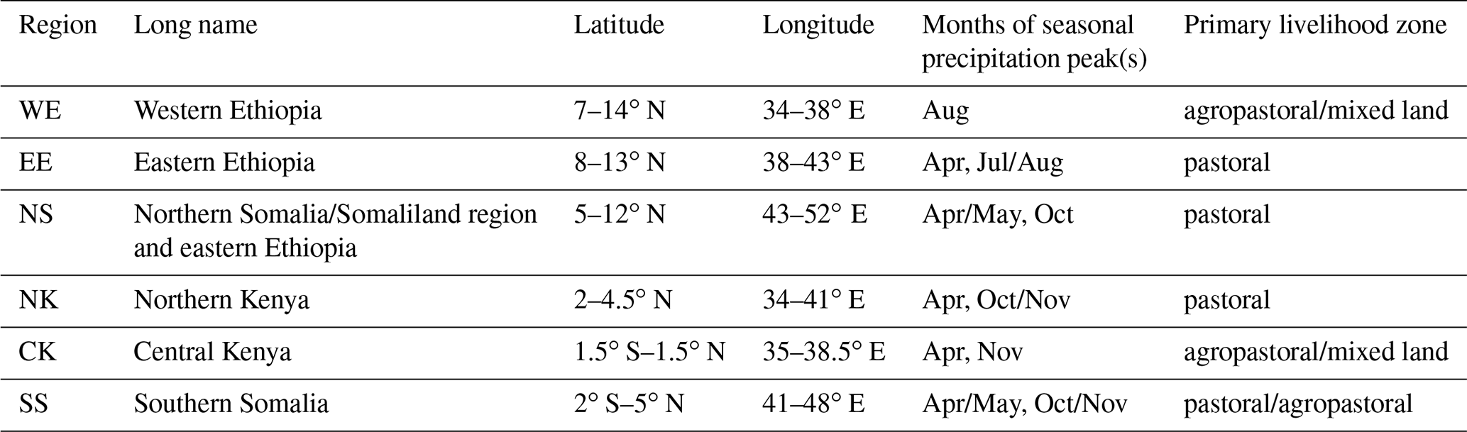
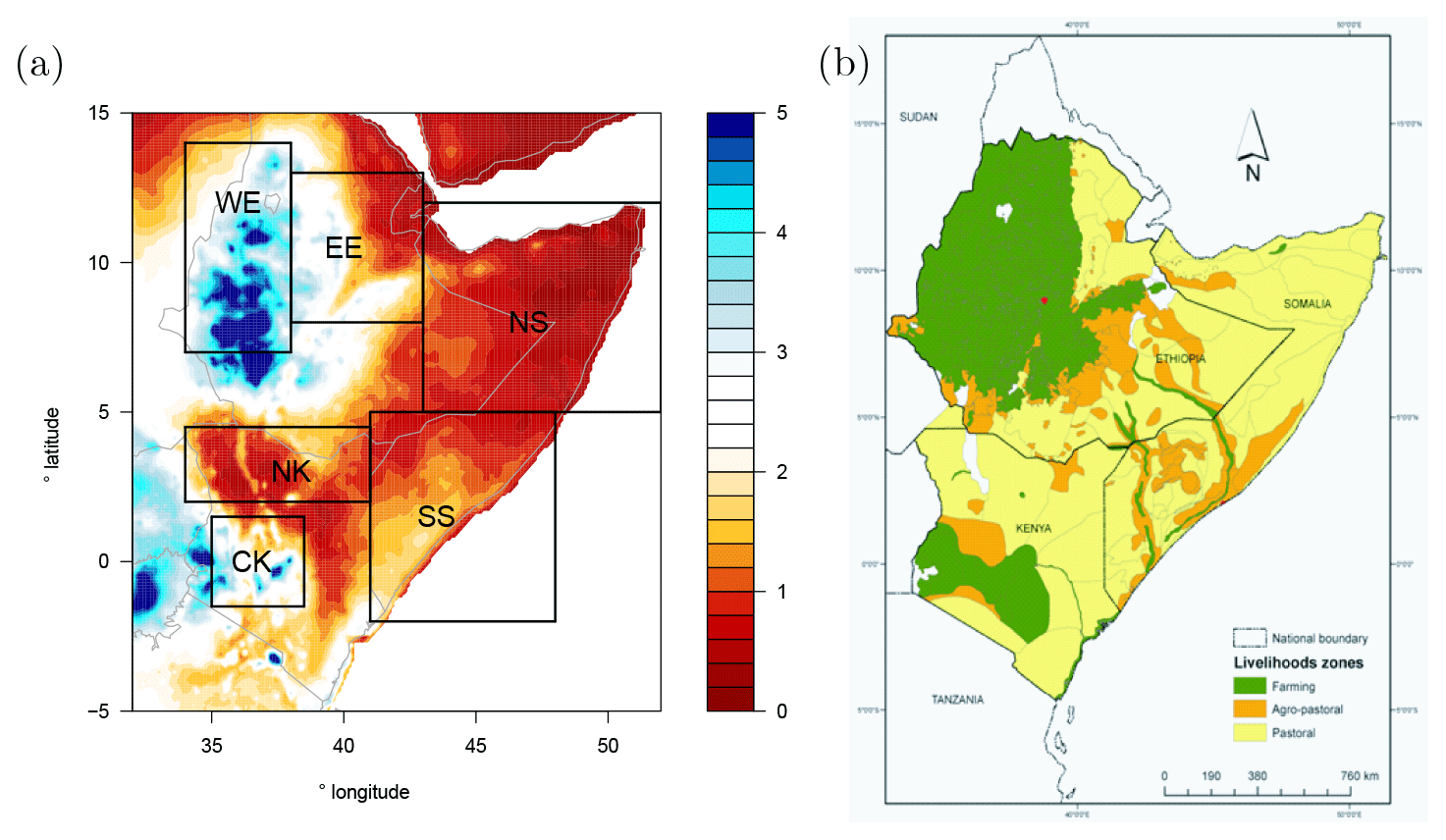
Figure 1(a) Annual mean precipitation [mm/d] and the six study regions. Note that only land values are used. (b) Livelihood zones, which were also used to define the study regions. Reprinted from Pricope et al. (2013) with permission from Elsevier.
2.2 Datasets
For the four study variables, we use all readily available datasets over the study area, provided that (i) the data are sufficiently complete over a period long enough to be used for trend calculations and (ii) the model data pass the validation tests (see Sect. 3). For this purpose, we use time series of at least 35 years. As the focus of this paper is on annual timescales, using monthly data is sufficient. The observational and model datasets used in this study are shown in Fig. 2 and listed in Tables 2 and 3 below (for brief descriptions of the projects from which these data originate, see the Supplement.) Note that we use the data as they are available without applying any additional bias correction, resampling or downscaling. Some of the data has undergone bias correction within their projects of origin, as described in the Supplement.
Funk et al. (2015)Harris et al. (2014)Rohde et al. (2013a, b)Dee et al. (2011)Bondeau et al. (2007); Rost et al. (2008); Schaphoff et al. (2013); Weedon et al. (2014)Sutanudjaja et al. (2018); Weedon et al. (2014)Oleson et al. (2010)Lawrence et al. (2011); Weedon et al. (2014)McNally et al. (2017)Hobbins et al. (2018)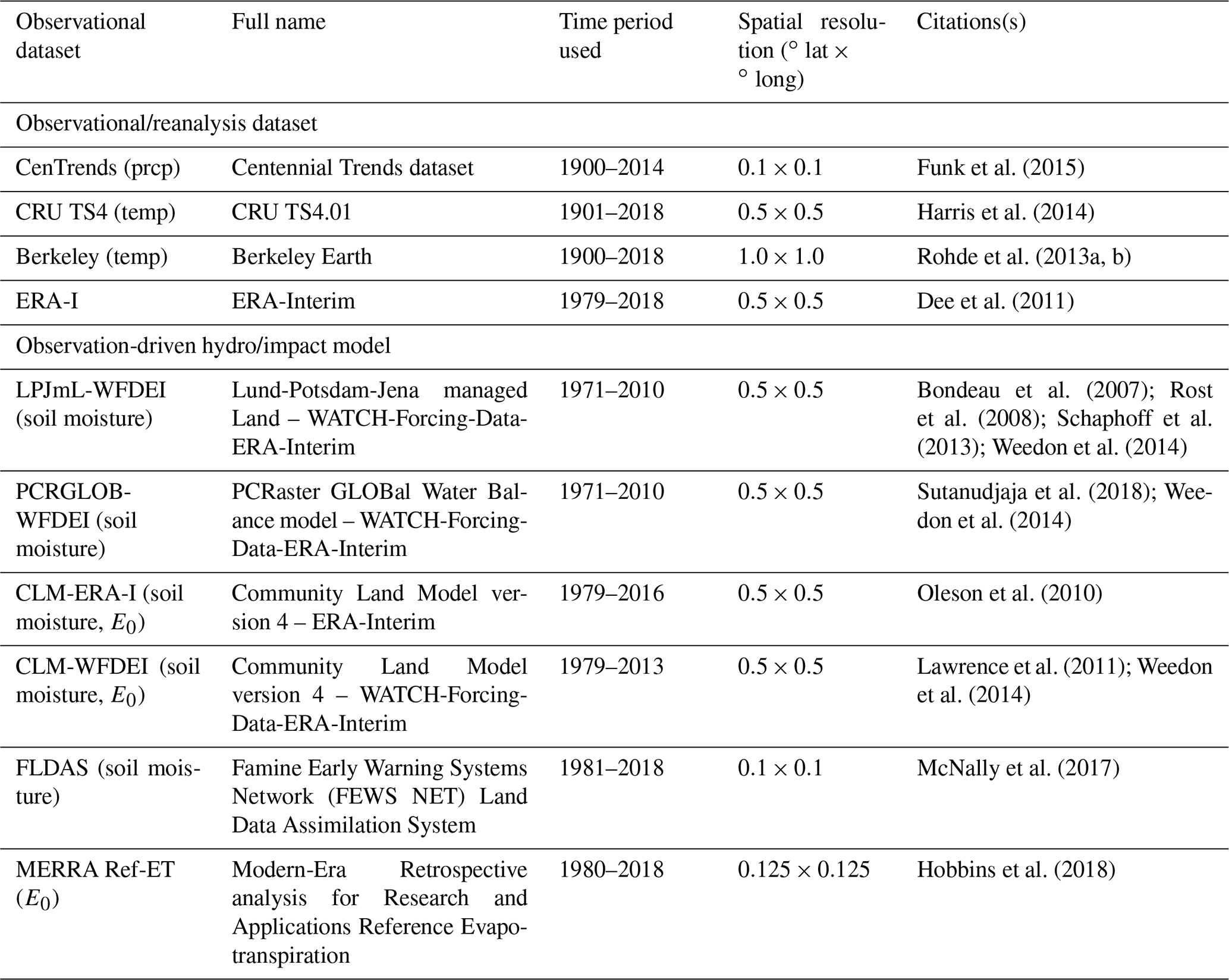
The following subsections address the observational datasets and modelling datasets in turn.
Observational datasets. For observations of precipitation and daily mean near-surface temperature, we use gridded observational datasets and reanalyses.
For soil moisture and E0, no direct observations meeting the above criteria exist. Instead, we use observational estimates of soil moisture and E0 resulting from various combinations of observational forcing data and models (see Fig. 2a).
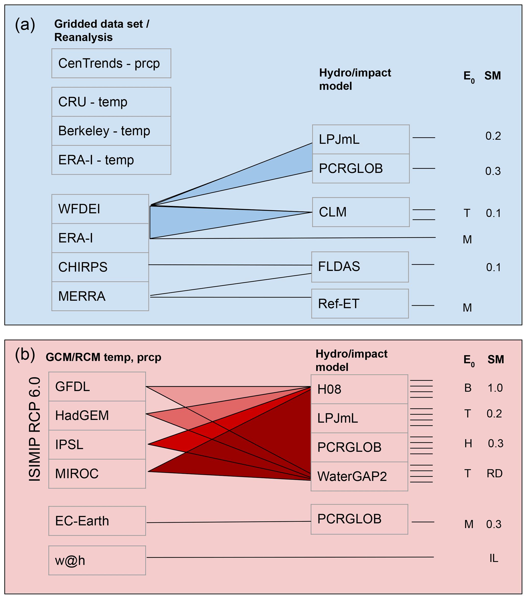
Figure 2Datasets used in this paper. (a) Observational precipitation (prcp) and near-surface temperature (temp) datasets and (b) models. Listed under E0 is the E0 scheme (T: Priestley–Taylor; M: Penman–Monteith; H: Hamon; B: bulk formula) and under SM is the depth of the top soil moisture layer available (RD: depends on rooting depth, 0.1–1.5 m for WaterGAP2; IL: integrated over all layers). Shading indicates an experiment with either multiple input datasets or multiple hydrological models. The number of resulting hydrological model simulations are indicated by horizontal lines on the right side of the figure.
Observational series of soil moisture are few, generally too short to use for trend analysis, and do not correlate well with reanalysis or model data over eastern Africa (McNally et al., 2016). It is therefore important to use multiple observationally forced model estimates to span the large uncertainties from inter-dataset differences. There being no a priori reason to favour one soil moisture dataset over another, we treat all resulting soil moisture datasets equally. For both observed and modelled soil moisture datasets, we use the topmost layer (see Fig. 2 for the depth of the topmost layer) provided by each dataset, except for the model weather@home where the available soil moisture variable is an integrated measure of all four layers of soil moisture, including the deep soil. Each time series is scaled to have a standard deviation of 1 in order to make comparisons in trends possible.
E0 is a function of temperature, humidity, solar radiation, and wind speed. Observational estimates of E0 used here originate from reanalysis datasets or reanalysis-driven impact models. For both observed and modelled E0, there are various parameterizations, ranging from simple temperature- or radiation-based schemes to sophisticated schemes based on all the aforementioned components. Whilst the Penman–Monteith scheme is often considered superior (e.g., Hobbins et al., 2016), one is often constrained from using a Penman–Monteith parameterization due either to the lack of accurate or reliable input data or because the choice of E0 parameterization within a given hydrological model setting is already prescribed, as in the ISIMIP ensemble. We thus chose to use a variety of E0 parameterizations (mostly the PET metric) and input datasets in order to cover the range of possible E0 values and trends in E0. The E0 scheme used by each dataset is noted in Fig. 2.
Modelled datasets. Most simulations stem from the ISIMIP project, which provides output of the variables under investigation for four different impact models driven by four different GCMs. These simulations are complemented by other readily available model runs (EC-Earth-PCRGLOB-WB and weather@home) with different (but compatible) framings.
Using these various observations and modelled datasets, we cover a wide range of different factors that influence E0 and soil moisture. The different factors include meteorological forcing, model choice, RCP scenario for the greenhouse gas concentration trajectory, E0 scheme, number of soil layers and depth of topsoil layer, dynamic vegetation modelling (LPJmL only), and transient versus time-slice runs (see Sect. 3).
Dunne et al. (2012, 2013)Collins et al. (2011); Jones et al. (2011)Dufresne et al. (2013)Watanabe et al. (2010)Hazeleger et al. (2012)Massey et al. (2015); Guillod et al. (2017)Hanasaki et al. (2008a, b)Bondeau et al. (2007); Rost et al. (2008); Schaphoff et al. (2013)Sutanudjaja et al. (2018)Müller Schmied et al. (2016)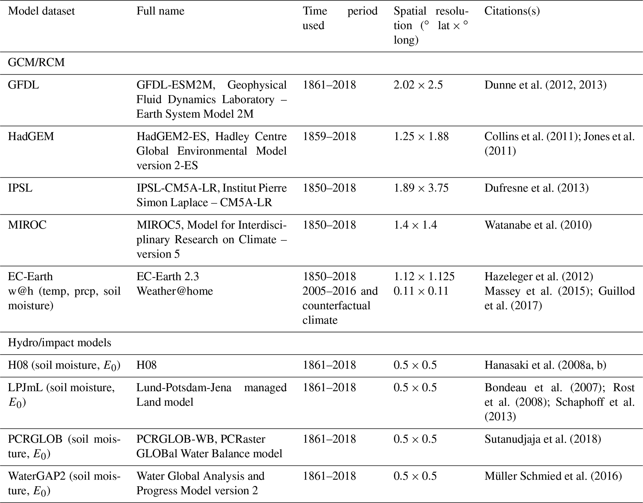
In this section, we first describe the method for detection and attribution of trends in the four variables, including model validation and the synthesis of observational and model results. Section 3.2 describes the assumptions and decisions that are made concerning the data and model setup, and Sect. 3.3 provides an example of how the method is applied to real data.
3.1 Detection and attribution of trends
In this section we detect trends in observations and analyse whether these trends, if present, can be attributed to human-induced climate change. In doing so, the approach taken to communicating uncertainty is as follows.
-
Perform a multi-model and multi-observation analysis that summarizes what we currently know using readily available data and methods.
-
Apply simple evaluation techniques to readily available data, treating datasets that satisfy evaluation criteria equally and rejecting the others.
-
Communicate uncertainties from synthesis. A simple “yes” or “no” is not appropriate if there is no significant trend. Instead, the uncertainties (confidence intervals) and their origin (e.g., natural variability or model spread) are given.
We use a multi-method, multi-model approach to address attribution. We use global mean surface temperature (GMST) as a measure for anthropogenic climate change for calculating trends. We calculate trends for all variables, regions and datasets and synthesize results into one overarching attribution statement for each of the four variables (soil moisture, precipitation, temperature, and E0) in each of the six regions. We use this method, following the approach applied in earlier studies on drought in eastern Africa (e.g., Philip et al., 2018a; Uhe et al., 2018) and other drought- and heat-attribution studies (e.g., Philip et al., 2018b; van Oldenborgh et al., 2018; Kew et al., 2019; Sippel et al., 2016), as it represents the current state of the art in extreme event attribution. The method is extensively explained in van Oldenborgh et al. (2021), Philip et al. (2020), van Oldenborgh et al. (2018), and van der Wiel et al. (2017).
In this study, for transient model runs and observational time series, we statistically model (i.e., fit) the dependency of annual means of the different variables on GMST (the model GMST for models and GISTEMP surface temperature GMST (Hansen et al., 2010) for observations and reanalyses) as follows.
After inspection of whether a Gaussian or a General Pareto Distribution fits the observational and reanalysis data best, we use the following distributions.
-
For soil moisture, a Gaussian distribution that scales with GMST, focussing on low values.
-
For precipitation, a General Pareto Distribution (GPD) that scales with GMST, analysing low extremes.
-
For temperature, a Gaussian distribution that shifts with GMST, focussing on high values.
-
For E0, a Gaussian distribution that scales with GMST, focussing on high values.
When the distribution is shifted, a linear trend α is fitted by making the location parameter μ dependent on GMST as
with α in [units of the study variable]/K. When the distribution is scaled,
which keeps the ratio of the location and scale parameter σ∕μ invariant. In each case, the fitted distribution is evaluated twice: once for the year 1900 and once for the year 2018. Confidence intervals (CI) are estimated using a non-parametric bootstrapping procedure. This allows us to calculate the return period of an event as if it had happened in the year 1900 or in the year 2018. To obtain a first-order approximation of the percentage change in the magnitude of the study variable between the 2 reference years, α is multiplied by 100 % times the change in GMST and divided by μ0 (for the shift fit this is exact). Note that for some variables – e.g., precipitation – it is appropriate to scale rather than shift the distribution with GMST (van Oldenborgh et al., 2021; Philip et al., 2020). For the very large weather@home ensemble simulations of actual and counterfactual climates, it is not necessary to use a fitting routine as the large amount of data permits a direct estimation of the trend. This also provides an opportunity to check the assumptions made in the fitting, notably that the values follow an extreme-value distribution and that the distribution shifts or scales with the smoothed GMST. We calculate trends for the time series of spatially and annually averaged data of all four variables and all six regions for all datasets by dividing the difference in the variable between the two ensembles by the difference in GMST.
Figures 3 and 4 present the methods applied to transient series and time slices, respectively. For reference and to aid interpretation of the return-period diagrams, the magnitude of a hypothetical event with a 20-year return period in the year 2018, i.e., in the current climate, is shown as a horizontal line or square. Reading the return period at which this line crosses the fit for the reference year 1900 shows how frequent an event with a 20-year return period in today's climate would have been at that time.
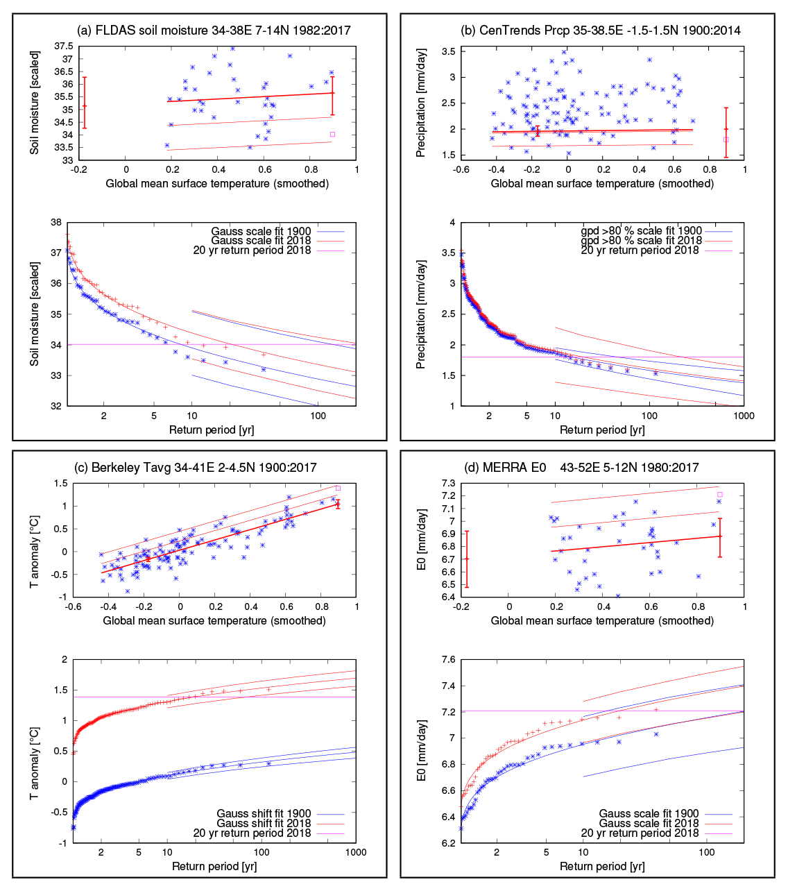
Figure 3Illustrative examples of the fitting method for each variable for selected study regions: (a) FLDAS soil moisture (Gaussian fit, low extremes, region WE); (b) CenTrends precipitation (GPD fit, low extremes, region CK); (c) Berkeley temperature anomaly (Gaussian fit, high extremes, region NK); (d) MERRA E0 (Gaussian fit, high extremes, region NS). At the top of each panel the following information is given: annually averaged data (stars) against GMST and fit lines – the location parameter μ (thick), μ±σ and μ±2σ (thin lines, Gaussian fits) and the 6- and 40-year return values (thin lines, GPD fit). Vertical bars indicate the 95 % confidence interval on the location parameter μ at the 2 reference years 2018 and 1900. The magenta square illustrates the magnitude of an event constructed to have a 20-year return period in 2018 (not included in the fit). At the bottom of each panel the following information is given: return period diagrams for the fitted distribution and 95 % confidence intervals, for the reference years 2018 (red lines) and 1900 (blue lines). The annually averaged data is plotted twice, being shifted or scaled with smoothed global mean temperature up to 2018 (red stars) and down to 1900 (blue stars). The magenta line illustrates the magnitude of a hypothetical event with a 20-year return period in 2018.
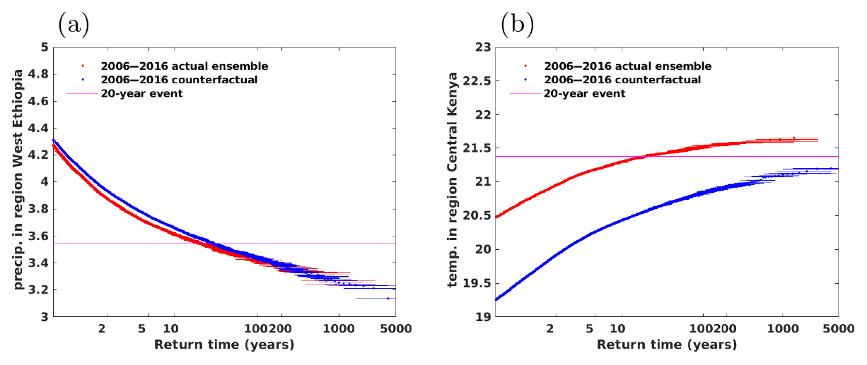
Figure 4Illustrative examples of the weather@home time slice model runs. (a) Annual mean precipitation [mm/d] in region WE. (b) Annual mean temperature [∘C] in region CK. The red markers are for the present-day climate and the blue markers are for the climate in pre-industrial times. The magenta line illustrates the magnitude of a hypothetical event with a 20-year return period in the present-day climate.
We only use results from model runs if they pass two different validation tests: a qualitative test on the seasonal cycle and a stronger test on variability. For soil moisture, due to the difficulties in obtaining reliable soil moisture measurements (e.g., Liu and Mishra, 2017) and the differences between the observational (reanalysis) datasets, we cannot assume that observational or reanalysis data are more accurate than model data. Therefore we simply use the soil moisture model data if the model input – precipitation and E0 – pass the validation tests.
We perform only a qualitative validation of the seasonal cycle. For each region, each variable, and each model we check that the seasonal cycle resembles that of at least one of the observational datasets, in terms of both the number and the timing of peaks. If the seasonal cycle is very different, we do not use the time series for that specific combination. This is the case for the original GCM precipitation in region NK for weather@home and in regions NK and CK for MIROC (the seasonal cycle is improved in the adjusted dataset, so we still use the time series in soil moisture) and for temperature in region SS for EC-Earth (we do not have adjusted data to check, so we do not use this model–region combination for soil moisture or E0).
The second validation test is on the model variability in precipitation and E0 (variability relative to the mean for variables that scale with GMST). If the model variability of a specific variable in a specific region is outside the range of variability calculated from observations or reanalyses, we do not use that specific dataset for that specific region and variable. For temperature, we relax the validation criteria on variability as it became clear during the analysis that the trend in soil moisture does not depend strongly on temperature and the trend in temperature agrees between models and observations. In two of the regions a strict validation resulted in only two driving GCMs. Trends from the resulting time series that passed the validation tests are shown in Sect. 4 and in the figures in the Supplement.
Using the large weather@home ensemble (which requires no fitting), we check the assumption that annual soil moisture and precipitation scale with GMST and temperature shifts with GMST. For E0, we assume that the distribution scales with GMST. In the weather@home ensemble, dry extremes show less change than intermediate dry extremes, which supports our assumption that scaling with GMST is appropriate (except for the higher return values, where the uncertainties are large). For soil moisture it is very difficult to distinguish between scaling and shifting from the weather@home ensemble because the trend is small. For temperature the weather@home ensembles indicate that the highest temperatures are increasing slower than the lower temperatures. This implies that the variability decreases with GMST; however, no consistent signal in the observations or other models is evident (we see a small increase in variability with time for Berkeley, a small decrease for CRU, and no consistency between the models). This does not significantly affect the trend, which is evaluated for the centre of the distribution.
Trends are presented as change in a variable per degree of GMST warming. We show trends rather than probability ratios, because we can derive finite ranges in confidence intervals for all variables. This is not the case for the probability ratio, where, for example, strong trends in temperature imply that mild extremes of the 2018 climate (e.g., a 1-in-20-year event) would have had a chance of almost zero around 1900, resulting in very large probability ratios and extensive extrapolation of the fit beyond the length of the dataset.
We synthesize the trends of all data that pass the validation tests in the following manner (see also Fig. 5). The observational (reanalysis) estimates are based on the same natural variability: the historical weather. They also cover similar time periods. The uncertainties due to natural variability (denoted as solid blue in the synthesis figures) are therefore highly correlated. We approximate these correlations by assuming the natural variability to be completely correlated and compute the mean and uncertainties as the average of the different observational estimates. The spread of the estimates is a measure of the representation uncertainty in the observational estimate and is added as an independent uncertainty to the natural variability (outlined black boxes). This results in a consolidated value for the observations (reanalyses) drawn in dark blue.
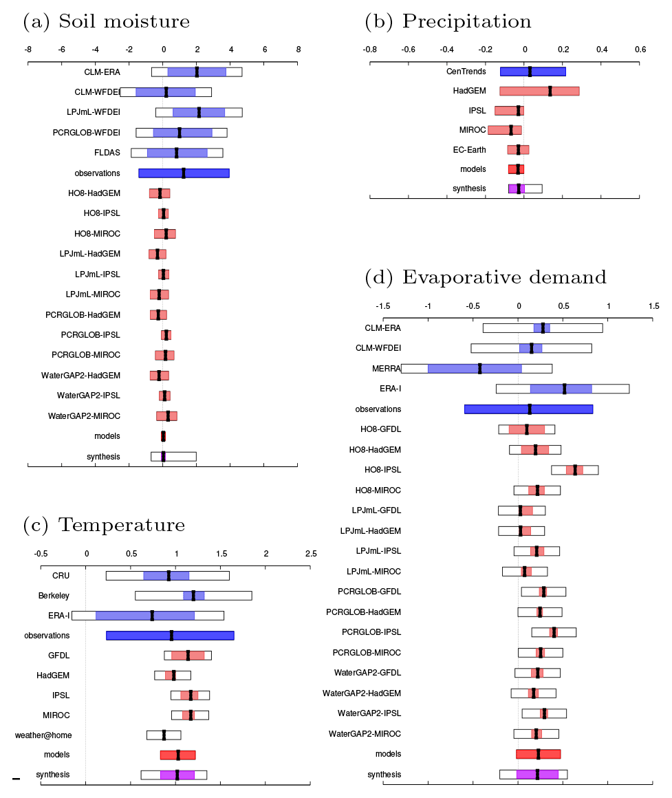
Figure 5Illustrative examples of the synthesized values of trends per 1 K GMST rise for soil moisture [/K] (a), precipitation [mm/d/K] (b), temperature [K/K] (c), and E0 [mm/d/K] (d) for region SS. Black bars are the average trends, coloured boxes denote the 95 % CI. Blue represents observations and reanalyses, red represents models, and magenta represents the weighted synthesis. Coloured bars denote natural variability, and white boxes also take representativity and model errors into account, if applicable (see Sect. 3). In the synthesis, the magenta bar denotes the weighted average of observations and models and the white box denotes the unweighted average. Soil moisture trends are based on standardized data; the other trends are absolute trends.
In contrast, model estimates have more uncorrelated natural variability: totally uncorrelated for coupled models and largely uncorrelated for SST-forced models (the predictability of annual mean precipitation given perfect SSTs is low in eastern Africa). We approximate these correlations by taking the natural variability to be uncorrelated. The spread of model results can be compared by the spread expected by the natural variability by computing the χ2∕dof statistic. If this is greater than one, there is a noticeable model spread, which is added in quadrature to the natural variability. This is denoted by the white boxes in Fig. 5. The bright red bar indicates the total uncertainty of the models, consisting of a weighted mean using the (uncorrelated) uncertainties due to natural variability plus an independent common model spread added to the uncertainty in the weighted mean.
Finally, observations and models are combined into a single result in two ways. Firstly, we compute the weighted average of the synthesized values for models and observations, neglecting model uncertainties beyond the model spread: this is indicated by the magenta bar. However, we know that models in general struggle to represent the climate of eastern Africa, so the model uncertainty is larger than the model spread. Therefore, we also use the more conservative estimate of an unweighted average of the synthesized values for observations and models, which gives more weight to the observations. This is indicated by the white box around the magenta bar. Whichever type of weighting is chosen, both the best estimate and uncertainty ranges are communicated.
3.2 Assumptions and decisions
We made the following assumptions and decisions about the data and model setup in addition to completing the model evaluation to attain data of sufficient quality.
-
The CenTrends precipitation dataset includes many different sources of precipitation data and more stations than most other datasets (Funk et al., 2015). We therefore assume it to be superior relative to other datasets over our study region; it is therefore our only source of observations of precipitation.
-
In general, we use the longest time series of data available. We make exceptions in the starting year based on visual inspection of abrupt changes due to data limitations toward the beginning of the time series.
- a.
We use Berkeley starting from 1900, except in region SS, where we start in 1920.
- b.
We use CRU starting from 1901, except in regions NK, CK, and SS, where we start in 1940.
- a.
-
Across our study region, no realistic soil moisture dataset exists covering a long-enough time period to calculate trends. Therefore we do not select simulations based on evaluation criteria other than selecting runs based on precipitation and E0 evaluation in the input variables.
-
As models do not share a consistent set of soil moisture levels, we take the top level of each model, assuming that this is the most comparable level across models. We checked for LPJmL – the only selected ISIMIP hydrological model that has more than one level available for soil moisture – that the variability does not change significantly when integrating over multiple levels instead of using level 1.
-
Within the ISIMIP project, variables required by the hydrological models, including precipitation and temperature, were bias-corrected and the adjusted data was used to calculate E0 and to drive the hydrological models to output soil moisture. In the synthesis, however, we present results for precipitation and temperature based on the unadjusted data, on the principle that this better spans the range of model uncertainty in these variables. The bias correction applied in ISIMIP aims to conserve the original trend (Hempel et al., 2013). Therefore, we find little change in trend for most time series.
-
In using our variety of E0 metrics, we do not convert reference evapotranspiration (such as that drawn from the MERRA-2 dataset (Hobbins et al., 2018) to PET, nor do we use crop coefficients to convert reference evapotranspiration to crop evapotranspiration because doing so would not be relevant to the research purposes. Our study is only interested in evaporative demand in its purest sense – i.e., as the atmospheric control driving upward moisture flux in the land–atmosphere system. In any case, crop coefficients we used would be (i) so inaccurate as to be meaningless at the large spatial scales of our analysis and (ii) different for each of the different metrics of E0 that we use. The ensemble of E0 values generated by our variety of E0 metrics will ensure that significant trends generated are robust.
-
We focus on the historical time frame. Therefore the trends in different RCP and socio-economic scenarios will be relatively similar to each other. The forcing data is the same for the years 1860–2005 and only differs for the most recent years from 2006 onwards. In general, however, using different scenarios can be seen as an advantage, as a greater range of scenario uncertainty will be spanned.
- a.
We use RCP6.0 in ISIMIP as this choice resulted in the largest number of simulations and RCP8.5 in EC-Earth as this was the only scenario available.
- b.
We selected the “historical” socio-economic scenario in ISIMIP model runs for 1860–2005 and “2005soc” for 2006–present; for H08, historical was unavailable for years 1860–2005, so we instead used 2005soc for those years and for years 2006–present. For the WFDEI experiments, 2005soc was unavailable, so we used historical before 2006 and “varsoc” for the years 2006–2018.
- a.
-
Trends are calculated or extrapolated using all data up to 2018 and between the pre-industrial era (1900) and the present (2018). Weather@home is an exception, where trends are calculated between two stationary climates of the present and the pre-industrial era. Differences in trends can arise due to different time periods and lengths of datasets, which are generally shorter for observational series and reanalyses than for model simulations. However, we consider the use of all available observational and reanalysis data and different model framings to lead to a more complete and robust attribution statement.
-
We analyse January–December annual means. Based on the seasonal cycles of precipitation and temperature, for all regions except for the region WE (which has a single rainy season) we could also have chosen to analyse July–June annual means instead. The influence of this choice on the trends is low (see also Sect. 3.3).
-
For consistency in the method, we fit the variability as a constant over time for all data. In both observed time series and simulations we see very little or no trend in variability up to 2018.
-
If for observational data a Gaussian fit is the best fit, we also fit model data to a Gaussian, even if a GPD is a better fit for that data. In doing this we avoid erroneous comparisons between the variable mean and variable extreme. We checked for model runs in which this disparity occurs but found that in most cases the trend calculated from fitting model data to a GPD was not very different from the trend calculated from fitting model data to a Gaussian.
3.3 Illustrative examples
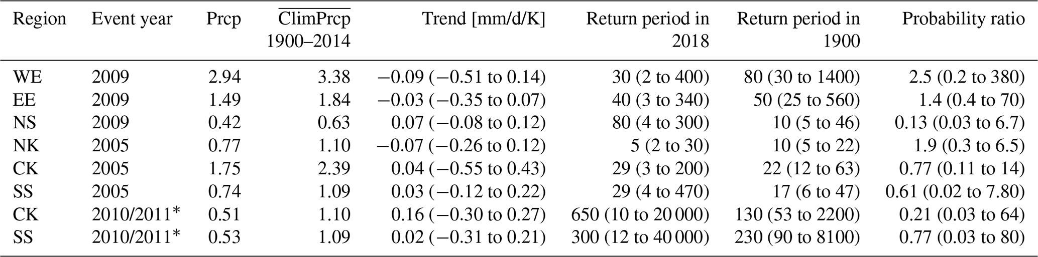
In this section we show an example to illustrate the method of detection of trends in precipitation data, as drought is often experienced as reduced or failed rainy seasons. For this purpose, we calculated return periods and risk ratios of recent droughts defined as low-precipitation events on an annual timescale (see Table 4). Note that the risk ratios are calculated from CenTrends alone and are not synthesized values based on a multi-model analysis. The synthesis of observations with models follows in the next section. We chose events based on the Emergency Events Database (EM-DAT) – an extensive global database of the occurrence of, and effects incurred from, extreme weather events – and the time series calculated from CenTrends (up to December 2014 only, which excludes the recent droughts of 2015 and 2016/2017). For the three northern study regions (WE, EE, and NS) we chose the year 2009, in which the first rainy season failed (in region WE, where there is only one peak in precipitation, the whole season had slightly lower precipitation amounts). For the southern three study regions (CK, NK, and NS) we choose the year 2005, in which the second rainy season failed. Additionally, we also investigated the well-known 2010/2011 drought for the regions NK and SS. As this drought occurred from late 2010 to early 2011 (the second part of 2011 was in fact very wet), we define the annual period of this specific 2010/2011 analysis to be July–June.
Taking region WE as an example, the results show that in CenTrends the trend in precipitation between 1900 and 2018 is −0.09 mm/d/K (95 % CI −0.51 to 0.14 mm/d/K). With a change in GMST of 1.07 K and a mean precipitation in 1900 of 3.2 mm/d, this is similar to a change of 3 %. Thus, if an event with the same precipitation amount as in the year 2009 had happened again in 2018 it would have been a 1-in-30-year event (95 % CI 2 to 400) in 2018, whereas in 1900 it would have been a 1-in-80-year event (95 % CI 30 to 1400), corresponding to a probability ratio of 2.5 (95 % CI 0.2 to 380). A return period that decreases in time indicates that such extreme droughts are becoming slightly more common; however, in this example we see large uncertainties consistent with no change. Note that the trend and probability ratio are not significantly different from zero at p < 0.05. The results for all regions are summarized in Table 4. (We note that the trends calculated for the January–December events and for the July–June events in regions NK and SS respectively are not significantly different. This supports the decision to analyse January–December annual extremes only.)
Table 4Trends, return periods, and probability ratios of equivalent events in the year 2018 and 1900 for three recent drought events registered in the EM-dat database (2005, 2009, and 2010/2011), based on annual average precipitation (mm/d) from the CenTrends dataset. The 95 % confidence intervals are given between brackets. For each study region impacted by the events, the annual precipitation for the event year (Prcp, used to define the event magnitude) and the 1900–2014 climatological precipitation average () is given. The asterisk * denotes that July–June is taken instead of January–December to define a year.
In this section, we illustrate the synthesis method. Intermediate synthesis figures, which show not only the overall synthesis but also the results for individual models, are presented for the region SS for each of the four variables; the intermediate synthesis figures of all six regions can be found in the Supplement. Table 5 and Fig. 6 summarize final synthesized findings for all regions. Using both the intermediate and final synthesis results, we first draw conclusions based on different GCMs and hydrological models and then turn to conclusions for each variable.
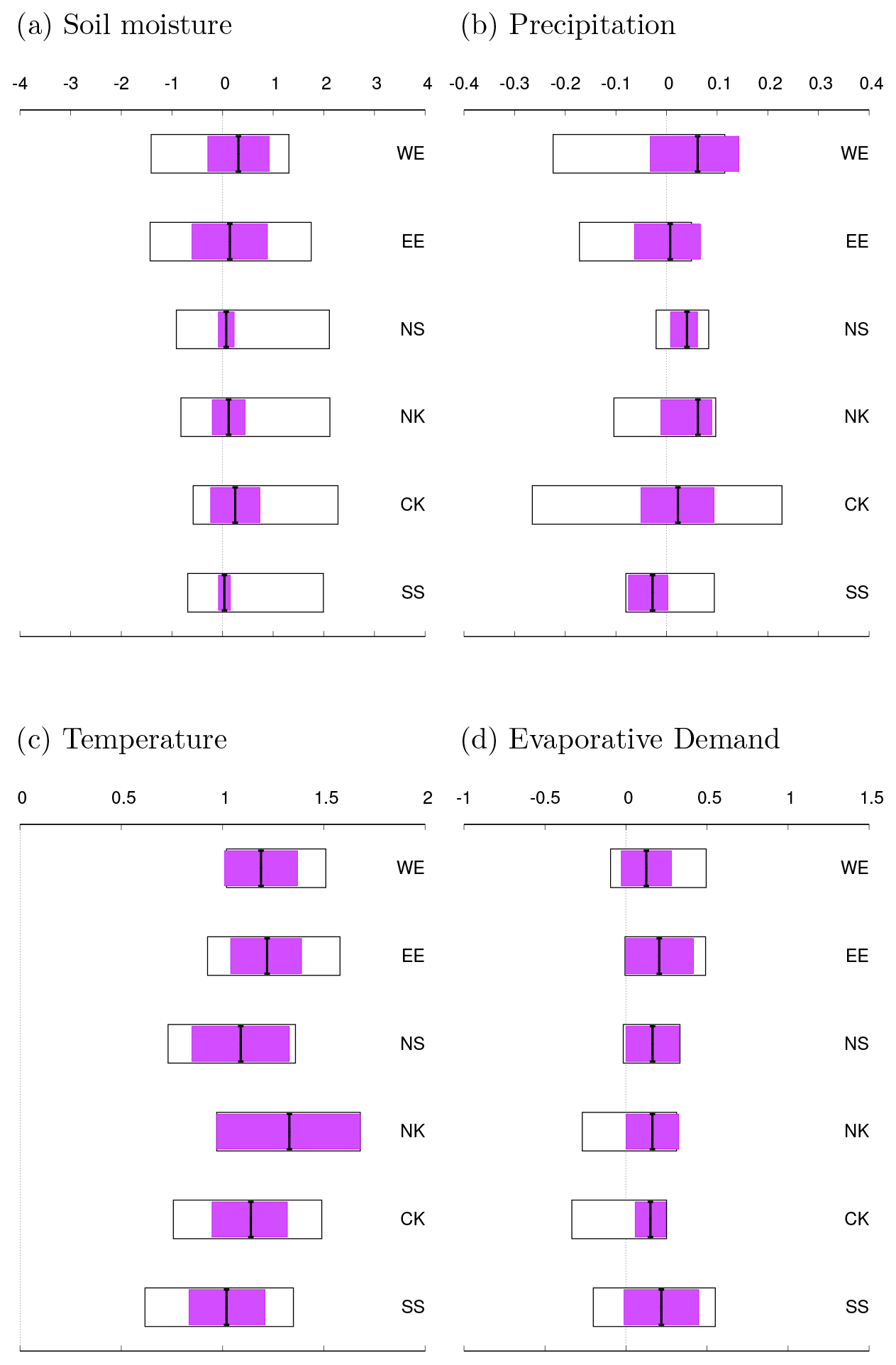
Figure 6Summary of the synthesized values for (a) soil moisture in [/K], (b) precipitation in [mm/d/K], (c) temperature in [K/K], and (d) E0 in [mm/d/K] in the six regions. The magenta bars denote the weighted averages of observations and models, and the white boxes denote the unweighted averages.
First, we look for consistent behaviour in the trends from individual GCMs across the four variables. We note that the results from low-resolution GCMs do not consistently stand out compared to higher-resolution models and also overlap with observational uncertainty. Some general conclusions about the different GCMs are as follows: (i) for GCM-driven model runs with stronger positive trends in temperature, there is a tendency for the positive trends in E0 also to be stronger and vice versa for weaker trends; (ii) the uncertainty in precipitation trends is high compared to the trend magnitudes, which partially explains why a clear relation with soil moisture trends is not evident; and (iii) no clear relation between local temperature trends and soil moisture trends is evident.
Looking at the different hydrological models, we conclude that the trend in PCR-GLOBWB E0, which uses the Hamon E0 scheme that depends only on temperature, is generally higher than the trend in EC-Earth E0, which uses the more complex Penman–Monteith E0 scheme that additionally depends on humidity, wind speed, and solar radiation. Using this more complex scheme can influence the trend in soil moisture, especially in wetter regions.
Table 5Summary of synthesis results for each region and study variable. Note that “0” means no significant change, a “+” sign indicates a positive trend, and a “−” sign indicates a negative trend. The uncertainties associated with each result are depicted in Fig. 6.
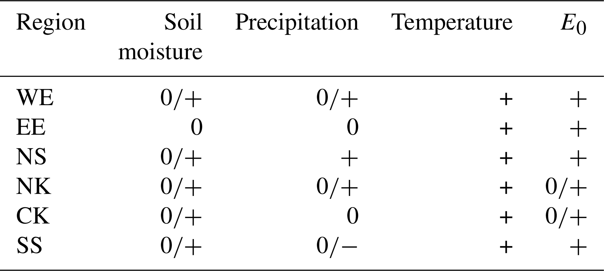
The analyses of the individual model runs, stratifying by GCM or hydrological model, do not lead to a clear conclusion on the relation between the trends in soil moisture, precipitation, temperature, and E0. We therefore turn to the analysis of the synthesized values (see Table 5 and Fig. 6 for a summary of the outcome and Figs. 5 and S1 to S6 in the Supplement for synthesis diagrams). Table 5 summarizes the interpretation of the synthesized results shown in Fig. 6. The more the magenta bar is centred in the white box, the better the models agree with observations and the more we trust our attribution statement.
For soil moisture we find no significant synthesized trends: there is practically no change in region EE and no trend to a small, positive but non-significant trend in regions WE, NS, NK, CK and SS.
For precipitation, regions WE and NK show a positive but non-significant trend, although in region WE models and observations only partially overlap. In region NS there is a small positive trend, regions EE and CK show no trend (for EE only with partial overlap of models and observations), and region SS shows a negative, non-significant trend.
As expected from global climate change, the local annually averaged temperatures all have a significant positive trend, with best estimates between 1.0 and 1.3∘ per degree of GMST increase. Related to this, trends in E0 are also positive in four of the six regions but lower than for temperature and generally have larger confidence intervals. The regions NK and CK are the exceptions. Although weighted averages show positive trends, models show tendencies opposite to the observations. This incompatibility renders the results uncertain.
We can identify the following relationships between different variables: (i) precipitation trends have a (small) influence on soil moisture trends in regions WE, NS, and NK; (ii) in regions WE, EE, NS, NK, and CK, temperature and E0 have no discernible influence on soil moisture trends; (iii) in region SS, the non-significant negative trend in precipitation does not lead to lower soil moisture and neither do the trends in temperature or E0. While it would be desirable to link the overall findings to differences in regional climate, the differences in the synthesized results between regions are too small relative to confidence intervals to be able to say anything meaningful. It was nevertheless necessary to divide the study area into homogeneous regions, so that extremes experienced within each region are representative for that region and inhomogeneity is not influencing the location of the occurrence of extremes.
In this section, we interpret our results in the light of how our choices and assumptions may have influenced the outcomes and we compare them to previous studies.
Whilst it may be preferable to use soil moisture as a drought indicator, observations and simulations of precipitation are more reliable in this region (Coughlan de Perez et al., 2019). Precipitation has a large influence on agricultural droughts and is therefore appropriate to use in attribution studies in eastern Africa, supplementing the analysis of soil moisture. The outcome of previous studies that have focussed on precipitation deficits only (e.g., Philip et al., 2018a; Uhe et al., 2018) are thus still relevant and compare well with our results, i.e., that no consistent significant trends in droughts are found. A comparison between seasonal cycles of the different variables (averaging the monthly means over recent decades) shows that the seasonal cycle of soil moisture is similar to that of precipitation in all six study regions. In contrast, the inverse seasonal cycle of temperature is not similar to that of soil moisture. Whether the E0 seasonal cycle reflects elements of the soil moisture cycle or not depends on the E0 scheme used: temperature- or radiation-based schemes show a seasonal cycle that is similar to that of temperature, whereas more advanced schemes reflect a mixture between the seasonal cycles of precipitation and temperature, as they also synthesize the seasonal cycle in humidity, which is strongly correlated to that of precipitation. We thus conclude that the influence of precipitation on soil moisture is higher than that of temperature or most E0 schemes. This is supported by the synthesized results that show negligible or no trends in soil moisture and precipitation, whereas the trends in temperature and E0 are strongly positive.
If temperature has an influence on trends in soil moisture (through E0), we expect to see that the positive trend in temperature is coupled to a drying soil moisture trend. As we average over the annual scale, we may miss parts of the season when this effect is strongest. Therefore, we selected a region and period outside the rainy season in which the seasonal peak in temperature corresponds to a dip in soil moisture (region CK, months February–March) to inspect sub-annual trends (not shown). Even then, we find that there is no negative trend in soil moisture accompanying the positive temperature trends.
We study drought trends on annual as opposed to sub-annual timescales, as long-term drought presents a greater risk for food security. On the annual timescale, we do not see strong explanatory relationships between the trends in the four studied variables (soil moisture, precipitation, temperature, and E0). To gain insight into the relationships between the variables, we additionally looked at correlations on a sub-annual timescale. Simple correlations between monthly soil moisture, precipitation, temperature, and E0 (not shown) support the conclusions of Manning et al. (2018) on the influence of precipitation and E0 on soil moisture at water limited sites in Europe. They found that at water-limited sites the influence of precipitation on soil moisture is much larger than that of temperature via E0. In our study, we find the same for the driest regions and the driest months in the wetter regions, and for the more temperature-based E0 schemes. This is presumably because temperature-based schemes (such as the Hamon approach) do not reflect land surface–atmosphere interactions as well as those that are also driven by humidity and wind speed (such as the Penman–Monteith approach) or, to a lesser degree, by radiation (such as the Priestley–Taylor approach).
Previous studies have shown that both the E0 scheme and their input data can have a large influence on E0 values (Trambauer et al., 2014; Wartenburger et al., 2018). We confirm this using the CLM-ERA-PT (Priestley–Taylor), CLM-WFDEI-PT, and CLM-ERA-PM (Penman-Monteith) datasets (not shown). In our study regions, E0 values are consistently higher when using PM than when using PT. The differences in trends in E0 using ERA or WFDEI input or using PT or PM input are sometimes significant. However, comparing study regions, there is no consistency in the difference; in four out of the six regions the PM data shows a higher trend than the PT data, and in four out of the six regions WFDEI data shows a higher trend than the ERA data.
A study by Rowell et al. (2015) discussed the possibility that climate model precipitation trends in East Africa are influenced by the inability of the models to reliably represent key physical processes. Rainy seasons in this region are governed by large-scale processes, such as El Niño-Southern Oscillation (ENSO) dynamics and the shifting of the Intertropical Convergence Zone (ITCZ). We view the tests we perform on seasonal cycle and frequency distributions, which provide some assurance that large-scale physical processes are reasonably well described, to be a minimum requirement for model validation. To improve the performance of models and to understand the discrepancies between models and observations, a much more thorough investigation into the models' representation of physical processes and feedbacks is required, such as demonstrated by James et al. (2018) and encouraged by the IMPALA (Improving Model Processes for African Climate) project (https://futureclimateafrica.org/project/impala/, last access: last access: 9 November 2018).
In the long term, a trend in E0 only has meaning for crop growth if there is water available for evapotranspiration. Much of eastern Africa is in a water-limited hydroclimate, requiring irrigation for crop growth. In irrigated areas within larger water-limited regions, the increased water availability shifts the local hydroclimate away from the surrounding water-limited regime towards a locally energy-limited regime. Positive trends in E0 seen in our analyses (especially if the variety of different schemes produces a robust E0 trend) could then signify a trend in actual ET and would therefore be accompanied by an increase in both irrigation water demand and, if that demand can be met, in crop growth. However, it should be noted that irrigation is not accounted for by the models or reanalysis datasets used here. Trends in E0 away from irrigated regions (i.e., in water-limited regions) will generally denote lower ET rates (through the complementary dynamics between E0 and ET that dominate in such regions), higher sensible heating of the atmosphere from a drier surface, and consequent greater drought exposure.
There are some factors influencing droughts and attribution results that are beyond the scope of this paper. For example, there is some evidence that warm spells are increasing in length, particularly in Ethiopia and the northern Somalia and Somaliland region (Gebrechorkos et al., 2019), as is the number of consecutive dry days in some parts of eastern Africa, which may have an impact on drought length and increase the rapidity of onset and the intensity of drought (Trenberth et al., 2014).
Furthermore, it is likely that increasing temperatures have a negative impact on food security during droughts through, e.g., decreased immunity of livestock, or increased water demand for cooling and water supply (Gebrechorkos et al., 2019, and references therein). In addition, in regions suffering from recent meteorological drought, non-meteorological factors such as increasing population and land-use changes also play a role in worsening the declining vegetation conditions, even after precipitation returns to normal (Pricope et al., 2013).
It is also still unknown how vegetation will respond to substantial increases in CO2 concentration. Two counteracting effects – physiological (restriction of stomatal openings leading to decreased evapotranspiration) and structural (increased leaf area leading to more stomata and increased evapotranspiration) responses – are expected, but their net effect is unknown (e.g., Wada et al., 2013). There are indications that “dynamic vegetation models” that include these CO2 effects show a weaker response of drought to climate change (Wada et al., 2013; Prudhomme et al., 2014). One of the hydrological models used in this study (LPJmL) uses dynamic vegetation modelling but there were no notable effects.
In this first multi-model, multi-method attribution study using several drought estimates in eastern Africa, we address the recurring question on whether increasing global temperatures exacerbate drought. Previous attribution studies for the eastern Africa region have examined drought from a meteorological perspective (precipitation deficit) and have found no clear trends above the noise of natural variability. In this study, we examined trends in eastern African drought from an agricultural perspective (soil moisture) as well as the meteorological perspective (precipitation, temperature, and E0 for six regions in eastern Africa. We also investigate whether global-warming-driven trends in these meteorological variables can be seen to contribute to trends towards drier soils. In this section, we draw conclusions for each variable in turn and make recommendations.
Of the four studied variables, soil moisture is most closely related to food security via crop health. In standardized soil moisture data, we found no discernible trends. The uncertainties in trends from model runs were found to be large, and there are no long observational runs available. This emphasizes that the use of an ensemble of models is imperative. Due to the large uncertainties in both soil moisture observations and simulations, we find no trend emerging from natural variability.
Precipitation was found to have a stronger influence than temperature or E0 on soil moisture variability, especially in the drier study regions (the significant positive trend in temperature is not reflected by a decrease in soil moisture). However, the confidence intervals on precipitation trend estimations are large and no clear trend is evident.
As expected from the increase in global temperatures, we find significant positive trends in local temperatures in all six regions. The synthesized trend is between 1.0 and 1.3 times the trend in GMST, which corresponds to a local temperature rise of 1.1 to 1.4∘ from pre-industrial times to 2018. However, the influence of this warming on annual soil moisture trends appears limited.
Soil moisture is more directly linked to E0 (via ET) than it is to temperature. Trends in E0 are predominantly positive, although in the regions NK and CK the uncertainty in this trend is large. This generally agrees with the positive trends in temperature. Similar to the results for temperature, we do not find strong relations between trends in E0 and soil moisture. Nevertheless, the results can still be of interest, both for irrigated regions where crop growth is limited only by meteorological conditions and for water-limited regions where the availability of water to evaporate greatly constrains forage growth. Due to large differences in results from different hydrological model runs, we recommend that E0 attribution analyses be carried out using an ensemble of hydrological models. These should use various (observational) input datasets and driving GCMs, although the decision to cover various E0 schemes is a trade-off between the desire to be representative of the uncertainty surrounding all approaches currently in use to not bias results towards a particular method (which is what we leant towards here by including, for example, the temperature-based Hamon approach) and the need to adhere to physical rigour in using the complete suite of drivers and an E0 parameterization that reflects all relevant dynamics (e.g., in the Penman–Monteith approach).
We conclude that although soil moisture is the preferred indicator of agricultural drought, we recommend that any soil moisture analysis be supplemented with precipitation analysis due to the superior reliability of precipitation measurements and the large influence of precipitation on drought in this region. Besides, soil moisture also has a physical lower limit: once the soil is dry it will remain dry. In water-limited regions an analysis of precipitation is thus a helpful addition.
Finally, communication of the uncertainties in the analyses of soil moisture, precipitation, temperature, and E0 (and any drought indicators) to policy makers, the media, and other stakeholders is crucial. Decision-makers need to properly weight and synthesize streams of potentially competing information from the variety of models, but without insight into the uncertainties in trends in the different drought indicators, they are missing this crucial information. They need to know how much the scientists trust their own conclusions, lest results be misinterpreted and conclusions become meaningless.
Almost all time series used in the analysis are available for download under https://climexp.knmi.nl/EastAfrica_timeseries.cgi (Kew and and Philip, 2019).
The supplement related to this article is available online at: https://doi.org/10.5194/esd-12-17-2021-supplement.
SFK and SYP designed and coordinated the study, analysed all data, and led the writing of the manuscript. MaH contributed the CLM datasets, including E0 calculations, and substantially contributed to writing. MiH produced the RefET dataset and substantially contributed to the writing. NW and KvdW collaborated to create the EC-Earth – PCR-GLOBWB data, including E0 calculations and bias correction. Niko Wanders additionally advised on the use and validation of E0 and soil moisture data for the analysis of drought. GJvO contributed analysis tools, monitored progress, and contributed to the writing. TIEV provided guidance on the use of ISIMIP data and contributed to discussions. JK and CF provided local information. FELO conceived the idea for the study, monitored development, provided weather@home results, and contributed to writing.
The authors declare that they have no conflict of interest.
For their roles in producing, coordinating, and making the ISI-MIP model output available, we acknowledge the modelling groups and the ISI-MIP coordination team. We would also like to thank the volunteers running the weather@home models and the technical team at OeRC for their support. MERRA-2 data were developed by the Global Modelling and Assimilation Office (GMAO) at the NASA Goddard Space Flight Center under funding from the NASA Modelling, Analysis, and Prediction (MAP) program; the data are disseminated through the Goddard Earth Science Data and Information Services Center (GES DISC), and preliminary data have been made available thanks to GMAO.
This research has been supported by the Children's Investment Fund Foundation (CIFF) (grant no. 1805-02753).
This paper was edited by Axel Kleidon and reviewed by two anonymous referees.
Bondeau, A., Smith, P., Zaehle, S., Schaphoff, S., Lucht, W., Cramer, W., Gerten, D., Lotze-Campen, H., Müller, C., Reichstein, M., and Smith, B.: Modelling the role of agriculture for the 20th century global terrestrial carbon balance, Glob. Change Biol., 13, 679–706, https://doi.org/10.1111/j.1365-2486.2006.01305.x, 2007. a, b
Collins, W. J., Bellouin, N., Doutriaux-Boucher, M., Gedney, N., Halloran, P., Hinton, T., Hughes, J., Jones, C. D., Joshi, M., Liddicoat, S., Martin, G., O'Connor, F., Rae, J., Senior, C., Sitch, S., Totterdell, I., Wiltshire, A., and Woodward, S.: Development and evaluation of an Earth-System model – HadGEM2, Geosci. Model Dev., 4, 1051–1075, https://doi.org/10.5194/gmd-4-1051-2011, 2011. a
Coughlan de Perez, E., van Aalst, M., Choularton, R., van den Hurk, B., Mason, S., Nissan, H., and Schwager, S.: From rain to famine: assessing the utility of rainfall observations and seasonal forecasts to anticipate food insecurity in East Africa, Food Secur., 11, 57–68, https://doi.org/10.1007/s12571-018-00885-9, 2019. a
Dee, D. P., Uppala, S. M., Simmons, A. J., Berrisford, P., Poli, P., Kobayashi, S., Andrae, U., Balmaseda, M. A., Balsamo, G., Bauer, P., Bechtold, P., Beljaars, A. C. M., van de Berg, L., Bidlot, J., Bormann, N., Delsol, C., Dragani, R., Fuentes, M., Geer, A. J., Haimberger, L., Healy, S. B., Hersbach, H., Hólm, E. V., Isaksen, L., Kållberg, P., Köhler, M., Matricardi, M., McNally, A. P., Monge-Sanz, B. M., Morcrette, J.-J., Park, B.-K., Peubey, C., de Rosnay, P., Tavolato, C., Thépaut, J.-N., and Vitart, F.: The ERA-Interim reanalysis: Configuration and performance of the data assimilation system, Q. J. Roy. Meteor. Soc., 137, 553–597, https://doi.org/10.1002/qj.828, 2011. a
Dufresne, J.-L., Foujols, M.-A., Denvil, S., Caubel, A., Marti, O., Aumont, O., Balkanski, Y., Bekki, S., Bellenger, H., Benshila, R., Bony, S., Bopp, L., Braconnot, P., Brockmann, P., Cadule, P., Cheruy, F., Codron, F., Cozic, A., Cugnet, D., de Noblet, N., Duvel, J.-P., Ethé, C., Fairhead, L., Fichefet, T., Flavoni, S., Friedlingstein, P., Grandpeix, J.-Y., Guez, L., Guilyardi, E., Hauglustaine, D., Hourdin, F., Idelkadi, A., Ghattas, J., Joussaume, S., Kageyama, M., Krinner, G., Labetoulle, S., Lahellec, A., Lefebvre, M.-P., Lefevre, F., Levy, C., Li, Z. X., Lloyd, J., Lott, F., Madec, G., Mancip, M., Marchand, M., Masson, S., Meurdesoif, Y., Mignot, J., Musat, I., Parouty, S., Polcher, J., Rio, C., Schulz, M., Swingedouw, D., Szopa, S., Talandier, C., Terray, P., Viovy, N., and Vuichard, N.: Climate change projections using the IPSL-CM5 Earth System Model: from CMIP3 to CMIP5, Clim. Dynam., 40, 2123–2165, https://doi.org/10.1007/s00382-012-1636-1, 2013. a
Dunne, J. P., John, J. G., Adcroft, A. J., Griffies, S. M., Hallberg, R. W., Shevliakova, E., Stouffer, R. J., Cooke, W., Dunne, K. A., Harrison, M. J., Krasting, J. P., Malyshev, S. L., Milly, P. C. D., Phillipps, P. J., Sentman, L. T., Samuels, B. L., Spelman, M. J., Winton, M., Wittenberg, A. T., and Zadeh, N.: GFDL's ESM2 Global Coupled Climate-Carbon Earth System Models. Part I: Physical Formulation and Baseline Simulation Characteristics, J. Climate, 25, 6646–6665, https://doi.org/10.1175/JCLI-D-11-00560.1, 2012. a
Dunne, J. P., John, J. G., Shevliakova, E., Stouffer, R. J., Krasting, J. P., Malyshev, S. L., Milly, P. C. D., Sentman, L. T., Adcroft, A. J., Cooke, W., Dunne, K. A., Griffies, S. M., Hallberg, R. W., Harrison, M. J., Levy, H., Wittenberg, A. T., Phillips, P. J., and Zadeh, N.: GFDL's ESM2 Global Coupled Climate-Carbon Earth System Models. Part II: Carbon System Formulation and Baseline Simulation Characteristics, J. Climate, 26, 2247–2267, https://doi.org/10.1175/JCLI-D-12-00150.1, 2013. a
Fan, Z.-X. and Thomas, A.: Decadal changes of reference crop evapotranspiration attribution: Spatial and temporal variability over China 1960–2011, J. Hydrol., 560, 461–470, https://doi.org/10.1016/j.jhydrol.2018.02.080, 2018. a
Funk, C., Nicholson, S. E., Landsfeld, M., Klotter, D., Peterson, P., and Harrison, L.: The centennial trends greater horn of Africa precipitation dataset, Scientific Data, 2, 150050, https://doi.org/10.1038/sdata.2015.50, 2015. a, b, c
Gebrechorkos, S. H., Hülsmann, S., and Bernhofer, C.: Changes in temperature and precipitation extremes in Ethiopia, Kenya, and Tanzania, Int. J. Climatol., 39, 18–30, https://doi.org/10.1002/joc.5777, 2019. a, b
Guillod, B. P., Jones, R. G., Bowery, A., Haustein, K., Massey, N. R., Mitchell, D. M., Otto, F. E. L., Sparrow, S. N., Uhe, P., Wallom, D. C. H., Wilson, S., and Allen, M. R.: weather@home 2: validation of an improved global–regional climate modelling system, Geosci. Model Dev., 10, 1849–1872, https://doi.org/10.5194/gmd-10-1849-2017, 2017. a
Hanasaki, N., Kanae, S., Oki, T., Masuda, K., Motoya, K., Shirakawa, N., Shen, Y., and Tanaka, K.: An integrated model for the assessment of global water resources – Part 1: Model description and input meteorological forcing, Hydrol. Earth Syst. Sci., 12, 1007–1025, https://doi.org/10.5194/hess-12-1007-2008, 2008a. a
Hanasaki, N., Kanae, S., Oki, T., Masuda, K., Motoya, K., Shirakawa, N., Shen, Y., and Tanaka, K.: An integrated model for the assessment of global water resources – Part 2: Applications and assessments, Hydrol. Earth Syst. Sci., 12, 1027–1037, https://doi.org/10.5194/hess-12-1027-2008, 2008b. a
Hansen, J., Ruedy, R., Sato, M., and Lo, K.: Global Surface Temperature Change, Rev. Geophys., 48, RG4004, https://doi.org/10.1029/2010RG000345, 2010. a
Harris, I., Jones, P., Osborn, T., and Lister, D.: Updated high-resolution grids of monthly climatic observations – the CRU TS3.10 Dataset, Int. J. Climatol., 34, 623–642, https://doi.org/10.1002/joc.3711, 2014. a
Hazeleger, W., Wang, X., Severijns, C., Ştefănescu, S., Bintanja, R., Sterl, A., Wyser, K., Semmler, T., Yang, S., Van den Hurk, B., van Noije, T., van der Linden, E., and van der Wiel, K.: EC-Earth V2.2: description and validation of a new seamless earth system prediction model, Clim. Dynam., 39, 2611–2629, 2012. a
Hempel, S., Frieler, K., Warszawski, L., Schewe, J., and Piontek, F.: A trend-preserving bias correction – the ISI-MIP approach, Earth Syst. Dynam., 4, 219–236, https://doi.org/10.5194/esd-4-219-2013, 2013. a
Hobbins, M. T., Shukla, S., McNally, A. L., McEvoy, D. J., Huntington, J. L., Husak, G. J., Funk, C. C., Senay, G. B., Verdin, J. P., Jansma, T., and Dewes, C. F.: What role does evaporative demand play in driving drought in Africa?, AGU Fall Meeting, San Francisco, CA, USA, 12–16 December 2016, GC43F-02, 2016. a
Hobbins, M. T., Dewes, C. F., McEvoy, D. J., Shukla, S., Harrison, L. S., Blakeley, S. L., McNally, A. L., and Verdin, J. P.: A new global reference evapotranspiration reanalysis forced by MERRA2: Opportunities for famine early warning, drought attribution, and improving drought monitoring, in: proceedings of the 98th annual meeting of the American Meteorological Society, Annual Meeting, Austin, TX, USA, 6–11 January 2018, p. 12, 2018. a, b
James, R., Washington, R., Abiodun, B., Kay, G., Mutemi, J., Pokam, W., Hart, N., Artan, G., and Senior, C.: Evaluating Climate Models with an African Lens, B. Am. Meteorol. Soc., 99, 313–336, https://doi.org/10.1175/BAMS-D-16-0090.1, 2018. a
Jones, C. D., Hughes, J. K., Bellouin, N., Hardiman, S. C., Jones, G. S., Knight, J., Liddicoat, S., O'Connor, F. M., Andres, R. J., Bell, C., Boo, K.-O., Bozzo, A., Butchart, N., Cadule, P., Corbin, K. D., Doutriaux-Boucher, M., Friedlingstein, P., Gornall, J., Gray, L., Halloran, P. R., Hurtt, G., Ingram, W. J., Lamarque, J.-F., Law, R. M., Meinshausen, M., Osprey, S., Palin, E. J., Parsons Chini, L., Raddatz, T., Sanderson, M. G., Sellar, A. A., Schurer, A., Valdes, P., Wood, N., Woodward, S., Yoshioka, M., and Zerroukat, M.: The HadGEM2-ES implementation of CMIP5 centennial simulations, Geosci. Model Dev., 4, 543–570, https://doi.org/10.5194/gmd-4-543-2011, 2011. a
Kew, S. F. and Philip, S. Y.: East African drought study, available at: https://climexp.knmi.nl/EastAfrica_timeseries.cgi, last access: 29 April 2019. a
Kew, S. F., Philip, S. Y., van Oldenborgh, G. J., van der Schrier, G., Otto, F. E., and Vautard, R.: The Exceptional Summer Heat Wave in Southern Europe 2017, B. Am. Meteorol. Soc., 100, 49–53, https://doi.org/10.1175/BAMS-D-18-0109.1, 2019. a
Lawrence, D. M., Oleson, K. W., Flanner, M. G., Thornton, P. E., Swenson, S. C., Lawrence, P. J., Zeng, X., Yang, Z.-L., Levis, S., Sakaguchi, K., Bonan, G. B., and Slater, A. G.: Parameterization improvements and functional and structural advances in Version 4 of the Community Land Model, J. Adv. Model. Earth Sy., 3, M03001, https://doi.org/10.1029/2011MS00045, 2011. a
Li, Z., Chen, Y., Yang, J., and Wang, Y.: Potential evapotranspiration and its attribution over the past 50 years in the arid region of Northwest China, Hydrol. Process., 28, 1025–1031, https://doi.org/10.1002/hyp.9643, 2014. a
Liu, D. and Mishra, A. K.: Performance of AMSR_E soil moisture data assimilation in CLM4.5 model for monitoring hydrologic fluxes at global scale, J. Hydrol., 547, 67–79, https://doi.org/10.1016/j.jhydrol.2017.01.036, 2017. a
Manning, C., Widmann, M., Bevacqua, E., van Loon, A. F., Maraun, D., and Vrac, M.: Soil Moisture Drought in Europe: A Compound Event of Precipitation and Potential Evapotranspiration on Multiple Time Scales, J. Hydrometeorol., 19, 1255–1271, https://doi.org/10.1175/JHM-D-18-0017.1, 2018. a, b
Massey, N., Jones, R., Otto, F. E. L., Aina, T., Wilson, S., Murphy, J. M., Hassell, D., Yamazaki, Y. H., and Allen, M. R.: weather@home – development and validation of a very large ensemble modelling system for probabilistic event attribution, Q. J. Roy. Meteor. Soc., 141, 1528–1545, https://doi.org/10.1002/qj.2455, 2015. a
McNally, A., Shukla, S., Arsenault, K. R., Wang, S., Peters-Lidard, C. D., and Verdin, J. P.: Evaluating ESA CCI soil moisture in East Africa, Int. J. Appl. Earth Obs., 48, 96–109, https://doi.org/10.1016/j.jag.2016.01.001, 2016. a
McNally, A., Arsenault, K., Kumar, S., Shukla, S., Peterson, P., Wang, S., Funk, C., Peters-Lidard, C. D., and Verdin, J. P.: A land data assimilation system for sub-Saharan Africa food and water security applications, Scientific Data, 4, 170012, https://doi.org/10.1038/sdata.2017.12, 2017. a
Müller Schmied, H., Adam, L., Eisner, S., Fink, G., Flörke, M., Kim, H., Oki, T., Portmann, F. T., Reinecke, R., Riedel, C., Song, Q., Zhang, J., and Döll, P.: Variations of global and continental water balance components as impacted by climate forcing uncertainty and human water use, Hydrol. Earth Syst. Sci., 20, 2877–2898, https://doi.org/10.5194/hess-20-2877-2016, 2016. a
Obada, E., Alamou, E. A., Chabi, A., Zandagba, J., and Afouda, A.: Trends and Changes in Recent and Future Penman-Monteith Potential Evapotranspiration in Benin (West Africa), Hydrology, 4, 38, https://doi.org/10.3390/hydrology4030038, 2017. a
Oleson, K. W., Lawrence, D. M., Bonan, G. B., Flanner, M. G., Kluzek, E., Lawrence, P. J., Levis, S., Swenson, S. C., Thornton, P. E., Dai, A., Decker, M., DIckinson, R., Feddema, J., Heald, C. L., Hoffman, F., Lamarque, J. F., Mahowald, N., Niu, G., Qian, T., Randerson, J., Running, S., Sakaguchi, K., Slater, A., Stockli, R., Wang, A., Yang, Z., Zeng, X., and Zeng, X.: Technical description of version 4.0 of the Community Land Model, NCAR Technical Note 257, National Center for Atmospheric Research, Boulder, CO, USA, https://doi.org/10.5065/D6FB50WZ, 2010. a
Philip, S., Kew, S. F., van Oldenborgh, G. J., Otto, F., O'Keefe, S., Haustein, K., King, A., Zegeye, A., Eshetu, Z., Hailemariam, K., Singh, R., Jjemba, E., Funk, C., and Cullen, H.: Attribution Analysis of the Ethiopian Drought of 2015, J. Climate, 31, 2465–2486, https://doi.org/10.1175/JCLI-D-17-0274.1, 2018a. a, b, c
Philip, S. Y., Kew, S. F., Hauser, M., Guillod, B. P., Teuling, A. J., Whan, K., Uhe, P., and van Oldenborgh, G. J.: Western US high June 2015 temperatures and their relation to global warming and soil moisture, Clim. Dynam., 50, 2587–2601, https://doi.org/10.1007/s00382-017-3759-x, 2018b. a
Philip, S., Kew, S., van Oldenborgh, G. J., Otto, F., Vautard, R., van der Wiel, K., King, A., Lott, F., Arrighi, J., Singh, R., and van Aalst, M.: A protocol for probabilistic extreme event attribution analyses, Adv. Stat. Clim. Meteorol. Oceanogr., 6, 177–203, https://doi.org/10.5194/ascmo-6-177-2020, 2020. a, b
Pricope, N. G., Husak, G., Lopez-Carr, D., Funk, C., and Michaelsen, J.: The climate-population nexus in the East African Horn: Emerging degradation trends in rangeland and pastoral livelihood zones, Global Environ. Change, 23, 1525–1541, https://doi.org/10.1016/j.gloenvcha.2013.10.002, 2013. a, b
Prudhomme, C., Giuntoli, I., Robinson, E. L., Clark, D. B., Arnell, N. W., Dankers, R., Fekete, B. M., Franssen, W., Gerten, D., Gosling, S. N., Hagemann, S., Hannah, D. M., Kim, H., Masaki, Y., Satoh, Y., Stacke, T., Wada, Y., and Wisser, D.: Hydrological droughts in the 21st century, hotspots and uncertainties from a global multimodel ensemble experiment, P. Natl. Acad. Sci. USA, 111, 3262–3267, https://doi.org/10.1073/pnas.1222473110, 2014. a
Rohde, R., Curry, J., Groom, D., Jacobsen, R., Muller, R. A., Perlmutter, S., Wickham, A. R. C., and Mosher, S.: Berkeley Earth Temperature Averaging Process, Geoinfor. Geostat.-An Overview, 1, 2, https://doi.org/10.4172/2327-4581.1000103, 2013a. a
Rohde, R., Muller, R., Jacobsen, R., Muller, E., and Perlmutter, S.: A New Estimate of the Average Earth Surface Land Temperature Spanning 1753 to 2011, Geoinfor. Geostat.-An Overview, 1, 1, https://doi.org/10.4172/2327-4581.1000101, 2013b. a
Rost, S., Gerten, D., Bondeau, A., Lucht, W., Rohwer, J., and Schaphoff, S.: Agricultural green and blue water consumption and its influence on the global water system, Water Resour. Res., 44, W09405, https://doi.org/10.1029/2007WR006331, 2008. a, b
Rowell, D. P., Booth, B. B. B., Nicholson, S. E., and Good, P.: Reconciling Past and Future Rainfall Trends over East Africa, J. Climate, 28, 9768–9788, https://doi.org/10.1175/JCLI-D-15-0140.1, 2015. a
Schaphoff, S., Heyder, U., Ostberg, S., Gerten, D., Heinke, J., and Lucht, W.: Contribution of permafrost soils to the global carbon budget, Environ. Res. Lett., 8, 014026, https://doi.org/10.1088/1748-9326/8/1/014026, 2013. a, b
Shongwe, M. E., van Oldenborgh, G. J., van den Hurk, B. J. J. M., and van Aalst, M. K.: Projected Changes in Mean and Extreme Precipitation in Africa under Global Warming. Part II: East Africa, J. Climate, 24, 3718–3733, https://doi.org/10.1175/2010JCLI2883.1, 2011. a
Sippel, S., Otto, F. E. L., Flach, M., and van Oldenborgh, G. J.: The Role of Anthropogenic Warming in 2015 Central European Heat Waves, B. Am. Meteorol. Soc., 97, 51–56, https://doi.org/10.1175/BAMS-D-16-0150.1, 2016. a
Sutanudjaja, E. H., van Beek, R., Wanders, N., Wada, Y., Bosmans, J. H. C., Drost, N., van der Ent, R. J., de Graaf, I. E. M., Hoch, J. M., de Jong, K., Karssenberg, D., López López, P., Peßenteiner, S., Schmitz, O., Straatsma, M. W., Vannametee, E., Wisser, D., and Bierkens, M. F. P.: PCR-GLOBWB 2: a 5 arcmin global hydrological and water resources model, Geosci. Model Dev., 11, 2429–2453, https://doi.org/10.5194/gmd-11-2429-2018, 2018. a, b
Trambauer, P., Dutra, E., Maskey, S., Werner, M., Pappenberger, F., van Beek, L. P. H., and Uhlenbrook, S.: Comparison of different evaporation estimates over the African continent, Hydrol. Earth Syst. Sci., 18, 193–212, https://doi.org/10.5194/hess-18-193-2014, 2014. a
Trenberth, K. E., Dai, A., Van Der Schrier, G., Jones, P. D., Barichivich, J., Briffa, K. R., and Sheffield, J.: Global warming and changes in drought, Nat. Clim. Change, 4, 17–22, https://doi.org/10.1038/nclimate2067, 2014. a
Uhe, P., Philip, S., Kew, S., Shah, K., Kimutai, J., Mwangi, E., van Oldenborgh, G. J., Singh, R., Arrighi, J., Jjemba, E., Cullen, H., and Otto, F.: Attributing drivers of the 2016 Kenyan drought, Int. J. Climatol., 38, 554–568, https://doi.org/10.1002/joc.5389, 2018. a, b, c
van der Wiel, K., Kapnick, S. B., van Oldenborgh, G. J., Whan, K., Philip, S., Vecchi, G. A., Singh, R. K., Arrighi, J., and Cullen, H.: Rapid attribution of the August 2016 flood-inducing extreme precipitation in south Louisiana to climate change, Hydrol. Earth Syst. Sci., 21, 897–921, https://doi.org/10.5194/hess-21-897-2017, 2017. a
van Loon, A., Gleeson, T., Clark, J., Van Dijk, A., Stahl, K., Hannaford, J., Di Baldassarre, G., Teuling, A., Tallaksen, L., Uijlenhoet, R., Hannah, D., Sheffield, J., Svoboda, M., Verbeiren, B., Wagener, T., Rangecroft, S., Wanders, N., and Van Lanen, H.: Drought in the Anthropocene, Nat. Geosci., 9, 89–91, https://doi.org/10.1038/ngeo2646, 2016. a
van Oldenborgh, G. J., Philip, S., Kew, S., van Weele, M., Uhe, P., Otto, F., Singh, R., Pai, I., Cullen, H., and AchutaRao, K.: Extreme heat in India and anthropogenic climate change, Nat. Hazards Earth Syst. Sci., 18, 365–381, https://doi.org/10.5194/nhess-18-365-2018, 2018. a, b
van Oldenborgh, G. J., Otto, F. E. L., Vautard, R., van der Wiel, K., Kew, S., Philip, S., King, A. L. F., Arrighi, J., Singh, R., and van Aalst, M.: Pathways and pitfalls in extreme event attribution, Climatic Change, in review, 2021. a, b
Wada, Y., Wisser, D., Eisner, S., Flörke, M., Gerten, D., Haddeland, I., Hanasaki, N., Masaki, Y., Portmann, F. T., Stacke, T., Tessler, Z., and Schewe, J.: Multimodel projections and uncertainties of irrigation water demand under climate change, Geophys. Res. Lett., 40, 4626–4632, 2013. a, b
Wartenburger, R., Seneviratne, S. I., Hirschi, M., Chang, J., Ciais, P., Deryng, D., Elliott, J., Folberth, C., Gosling, S. N., Gudmundsson, L., Henrot, A.-J., Hickler, T., Ito, A., Khabarov, N., Kim, H., Leng, G., Liu, J., Liu, X., Masaki, Y., Morfopoulos, C., Müller, C., Schmied, H. M., Nishina, K., Orth, R., Pokhrel, Y., Pugh, T. A. M., Satoh, Y., Schaphoff, S., Schmid, E., Sheffield, J., Stacke, T., Steinkamp, J., Tang, Q., Thiery, W., Wada, Y., Wang, X., Weedon, G. P., Yang, H., and Zhou, T.: Evapotranspiration simulations in ISIMIP2a – Evaluation of spatio-temporal characteristics with a comprehensive ensemble of independent datasets, Environ. Res. Lett., 13, 075001, https://doi.org/10.1088/1748-9326/aac4bb, 2018. a
Watanabe, M., Suzuki, T., O'ishi, R., Komuro, Y., Watanabe, S., Emori, S., Takemura, T., Chikira, M., Ogura, T., Sekiguchi, M., Takata, K., Yamazaki, D., Yokohata, T., Nozawa, T., Hasumi, H., Tatebe, H., and Kimoto, M.: Improved Climate Simulation by MIROC5: Mean States, Variability, and Climate Sensitivity, J. Climate, 23, 6312–6335, https://doi.org/10.1175/2010JCLI3679.1, 2010. a
Weedon, G. P., Balsamo, G., Bellouin, N., Gomes, S., Best, M. J., and Viterbo, P.: The WFDEI meteorological forcing data set: WATCH Forcing Data methodology applied to ERA-Interim reanalysis data, Water Resour. Res., 50, 7505–7514, https://doi.org/10.1002/2014WR015638, 2014. a, b, c
Wilhite, D. and Glantz, M.: Understanding the Drought Phenomenon: The Role of Definitions, Water Int., 10, 111–120, 1985. a
Yin, Y., Wu, S., Chen, G., and Dai, E.: Attribution analyses of potential evapotranspiration changes in China since the 1960s, Theor. Appl. Climatol., 101, 19–28, https://doi.org/10.1007/s00704-009-0197-7, 2010. a