Storylines of weather-induced crop failure events under climate change

Unfavourable weather is a common cause for crop failures all over the world. Whilst extreme weather conditions may cause extreme impacts, crop failure commonly is induced by the occurrence of multiple and combined anomalous meteorological drivers. For these cases, the explanation of conditions leading to crop failure is complex, as the links connecting weather and crop yield can be multiple and non-linear. Furthermore, climate change is likely to perturb the meteorological conditions, possibly altering the occurrences of crop failures or leading to unprecedented drivers of extreme impacts. The goal of this study is to identify important meteorological drivers that cause crop failures and to explore changes in crop failures due to global warming. For that, we focus on a historical failure event, the extreme low soybean production during the 2012 season in the midwestern US. We first train a random forest model to identify the most relevant meteorological drivers of historical crop failures and to predict crop failure probabilities. Second, we explore the influence of global warming on crop failures and on the structure of compound drivers. We use large ensembles from the EC-Earth global climate model, corresponding to present-day, pre-industrial +2 and 3 ^∘C warming, respectively, to isolate the global warming component. Finally, we explore the meteorological conditions inductive for the 2012 crop failure and construct analogues of these failure conditions in future climate settings. We find that crop failures in the midwestern US are linked to low precipitation levels, and high temperature and diurnal temperature range (DTR) levels during July and August. Results suggest soybean failures are likely to increase with climate change. With more frequent warm years due to global warming, the joint hot–dry conditions leading to crop failures become mostly dependent on precipitation levels, reducing the importance of the relative compound contribution. While event analogues of the 2012 season are rare and not expected to increase, impact analogues show a significant increase in occurrence frequency under global warming, but for different combinations of the meteorological drivers than experienced in 2012. This has implications for assessment of the drivers of extreme impact events.

1 Introduction

Soybeans are important for modern global society. They are used for human consumption, the main source of protein for animal feed worldwide and the second most consumed type of vegetable oil (Hartman et al., 2011). The vast majority of its production is concentrated in specific regions in Argentina, Brazil and United States of America, accounting for 80 % of the world production (Hartman et al., 2011; Maria et al., 2020). The difference in scale between local production and global consumption makes soybeans the most traded crop in value in the world (FAO, 2021). Such a broad and extensive trade network renders the soybean supply chain especially vulnerable to local perturbations at the growing regions. Local shocks on production sites can potentially have worldwide consequences, as evidenced by the 2012 season, when exceptional low yields in most of the midwestern United States drove global soybean prices to the highest values ever recorded (Zhang et al., 2018).

Weather and climate events have direct influence on agricultural production (IPCC, 2012). On a global level, interannual climate variability is responsible for approximately 30 % of the year-to-year variability in crop yields (Lobell and Field, 2007), but the influence of interannual climate variability reaches up to 60 % of the yield variability in certain regions (Ray et al., 2015; Frieler et al., 2017). Extreme weather events are also linked to crop failures (Vogel et al., 2019). In addition, unprecedented weather conditions due to anthropogenic global warming may alter crop failure frequency and the climatic drivers behind failures. Recent warming trends are already impacting crops worldwide in multiple ways and further warm conditions are expected to exacerbate these impacts (Schauberger et al., 2017; Moore and Lobell, 2015; Ray et al., 2019; Zhao et al., 2017; Wolski et al., 2020; Iizumi and Ramankutty, 2016; Zhu and Troy, 2018).

While extreme weather events, such as abnormally low levels of precipitation or excessive heat, can alone cause disruptions of crop development (Deryng et al., 2014), the majority of climate-driven societal or natural shocks are the result of compound events (Zscheischler et al., 2017; Zampieri et al., 2017). Compound events are combinations of multiple climate drivers that lead to an extreme impact, without necessarily being extreme themselves (Leonard et al., 2014; Zscheischler et al., 2018). Compound events should ideally be assessed from an impact perspective or the analysis should at least account for the complexity of weather-impact relations, rather than relying exclusively on extreme weather states (Zscheischler and Fischer, 2020; van der Wiel et al., 2020). Dealing with this complexity requires the use of explicit models (van den Hurk et al., 2015; van der Wiel et al., 2020), and a common alternative is to use statistical models to represent compound events. From linear models (Ben-Ari et al., 2018; Vogel et al., 2021) to deep neural networks (Crane-Droesch, 2018), statistical models in climate studies have been successful in linking extreme impacts to weather and in explaining specific unusual events.

Explaining individual events is part of the event attribution domain. It aims to determine both the influence of random weather and the footprint of climate change in individual cases (Trenberth et al., 2015; van Oldenborgh et al., 2021). Storylines of climatic events that lead to high impacts may be used to explore complex events, related drivers and interactions, improving risk awareness and strengthening decision making (Shepherd et al., 2018). Storylines start from a given impact, be it historical or physically plausible, and create a physically sound chain of events from the impact to the driving components (Shepherd et al., 2018). The advantages of this approach are to quantify and understand the driving components and the influence of climate change and also the possibility of perturbing the driving components for the creation of analogues. Analogues are alternative realisations of a reference event that are perturbed by hypothetical conditions. Storylines can naturally embed the complexity of compound events and offer a framework to explore future analogues under different global warming scenarios (Shepherd, 2019). Since crop failures are usually the result of compound meteorological drivers, storylines can be built from a historical crop season of interest in order to disentangle the driving components and to generate analogues of the historical season under influence of climate change.

There are many recent studies that explore the interactions between crop and climate (Gawȩda et al., 2020; Zipper et al., 2016; Heino et al., 2018; Iizumi et al., 2014; Zampieri et al., 2017; Ogutu et al., 2018). Some have included the possible impacts of global warming under different scenarios (Rosenzweig et al., 2014; Lobell and Tebaldi, 2014; Feng et al., 2019; Xie et al., 2018). Others aimed to represent the compound nature of crop failures (Ben-Ari et al., 2018; van der Wiel et al., 2020; Vogel et al., 2021; Hamed et al., 2021; Zhu et al., 2021). van der Wiel et al. (2020) show the complexity between climate and crops by explicitly modelling the full distribution of climate impacts on crops with a physical crop model and large ensembles of climatic data. They demonstrate that links between extreme weather and extreme impacts are non-linear and the need for modelling impacts. Vogel et al. (2021) apply a statistical linear model to automatically identify the most relevant meteorological variables for simulated extreme impact events in large ensemble crop data. They conclude that compounding effects are ubiquitous across time and meteorological drivers for crop failures. Hamed et al. (2021) use a statistical linear model to identify dominant within season climatic drivers that influence soybean yield variability in the US and highlight the synergistic effects between summer heat and moisture conditions modulating the final impact on yields. They find that, in spite of beneficial summer wetting and cooling in the Midwest region largely attributed to agricultural intensification, the frequency of damaging joint hot and dry conditions remains largely unchanged. Ben-Ari et al. (2018) also apply a statistical linear model to successfully link climatic conditions with crop failures, including the identification of an extreme season that was not detected by the existing forecast models. Moreover, they individually analyse the trends for each of the selected meteorological variables for different levels of global warming. Building on these works, we expand the studies of global warming impacts on agriculture to include multivariate analysis by explicitly modelling the compound nature of meteorological variables and their interactions.

The aim of this work is to understand how global warming affects the meteorological conditions leading to crop failures. More specifically, we explain historical soybean failures, explore possible future analogues and assess changes in the compound drivers due to rising temperatures. The work is divided into three parts (Fig. 1): first, we develop a statistical model that links soybean failures generated by a crop model to local meteorological conditions. We use a non-linear and non-parametric statistical model (random forest) that accounts for compound drivers and that allows interpretation of the driving conditions (Fig. 1a). Second, we apply the model to 6000 years of climate data under different scenarios of global warming for failure analysis (Fig. 1b). Third, we evaluate analogues of the 2012 season in the global warming scenarios using two different approaches (Fig. 1c). Details on features selection, model training and the setup for the future analogues, along with the data used for this work, are presented in Sect. 2. The selected features are shown in Sect. 3.1, while the performance of the model and the explanation of the driving components are demonstrated in Sect. 3.2. The use of large ensembles for global warming scenarios and the role of compound events for crop failures are found in Sect. 3.3, while the exploration of analogues of the 2012 season is shown in Sect. 3.4. The findings are put into context and debated in Sect. 4, and a summary of the work with its main messages is presented in Sect. 5.

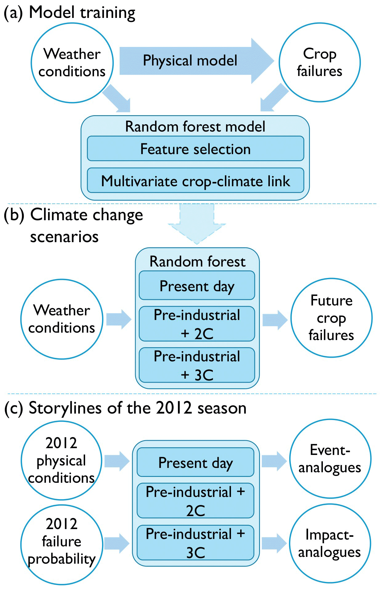
Figure 1 Experimental outline for this work. (a) Model training: the process of training a random forest model to link multiple local meteorological variables to crop failures. (b) Climate change scenarios: the extension of the trained random forest model for global warming scenarios to predict future soybean failure ratios. (c) Storylines of the 2012 season: construction of analogues to the 2012 season using two different approaches: the event analogues and the impact analogues.

2 Data and methods

2.1 Weather and crop data

We constructed a random forest (RF) model that identifies relationships between crop development and meteorological variables during the growing season. For crop data, we adopted yearly soybean yields (t/ha of dry matter) generated by the global gridded crop model (GGCM) EPIC-IIASA (Balkovič et al., 2014), which is based on the Environmental Policy Integrated Climate (EPIC; Williams et al., 1995) field-scale crop model. This GGCM simulates complex relations between weather conditions and crops at planetary scales by reproducing biophysical processes in the soil–plant–atmosphere system and providing crop-related outputs based on climate-related inputs. Simulation outputs used in this study were performed for phase 3a of the Intersectoral Impact Model Intercomparison Project (ISIMIP; see https://isimip.org, last access: 20 June 2021, for details and protocols) and the Global Gridded Crop Model Intercomparison (GGCMI) initiative. It used as climatic input in the GSWP3-W5E5 dataset, which is a merger of the GSWP3 (Global Soil Wetness Project phase 3) dataset (Dirmeyer et al., 2006) and the W5E5 dataset (Lange, 2019). It captures the period from 1901 to 2016 at a $\mathrm{0.5}{}^{\circ }\times \mathrm{0.5}{}^{\circ }$ resolution. The reasons for using yields from crop models are the longer time series that allow for more years to be included in the training of the statistical model and uniformity of data quality for regions where there is low quality of observational data. Another advantage of using simulated crop models is that management and technology trends are static, whereas they are intrinsically embedded in the observed yield datasets. Other works have also adopted simulated yields for climate–crop analysis (Vogel et al., 2021; Zhu et al., 2021). Details of the EPIC-IIASA model's performance can be seen in Folberth et al. (2016), Müller et al. (2019). We used 100 years of data (1916 to 2016) to train the model and we limited the analysis to grid cells from the top 10 US soybean producer states, which are (ordered by production volume): Illinois, Iowa, Minnesota, Indiana, Nebraska, Ohio, South Dakota, North Dakota, Missouri and Arkansas. Together, they represent over 70 % of the US national soybean production and approximately 20 % of the global soybean production (FAO, 2021). In addition, to ensure only rainfed soybeans were considered, we selected only grid cells that contained at least 90 % of the grid as rainfed, which corresponded to 84 % of the region studied (MIRCA2000; Portmann et al., 2010). For validation of the crop model, we compared the EPIC-IIASA simulated yields with the observed yields from the US Department of Agriculture (USDA, https://www.nass.usda.gov/Quick_Stats/, last access: 15 August 2021) for the region considered. EPIC-IIASA has higher mean and standard deviations values than the observed because the simulated yields are potential (Folberth et al., 2016). To evaluate the interannual variability, we obtained a coefficient of determination, R², of 0.674. We also observed a good correlation between the two standardised datasets (Fig. C1). We consider EPIC capable of replicating the interannual variability of the observed data.

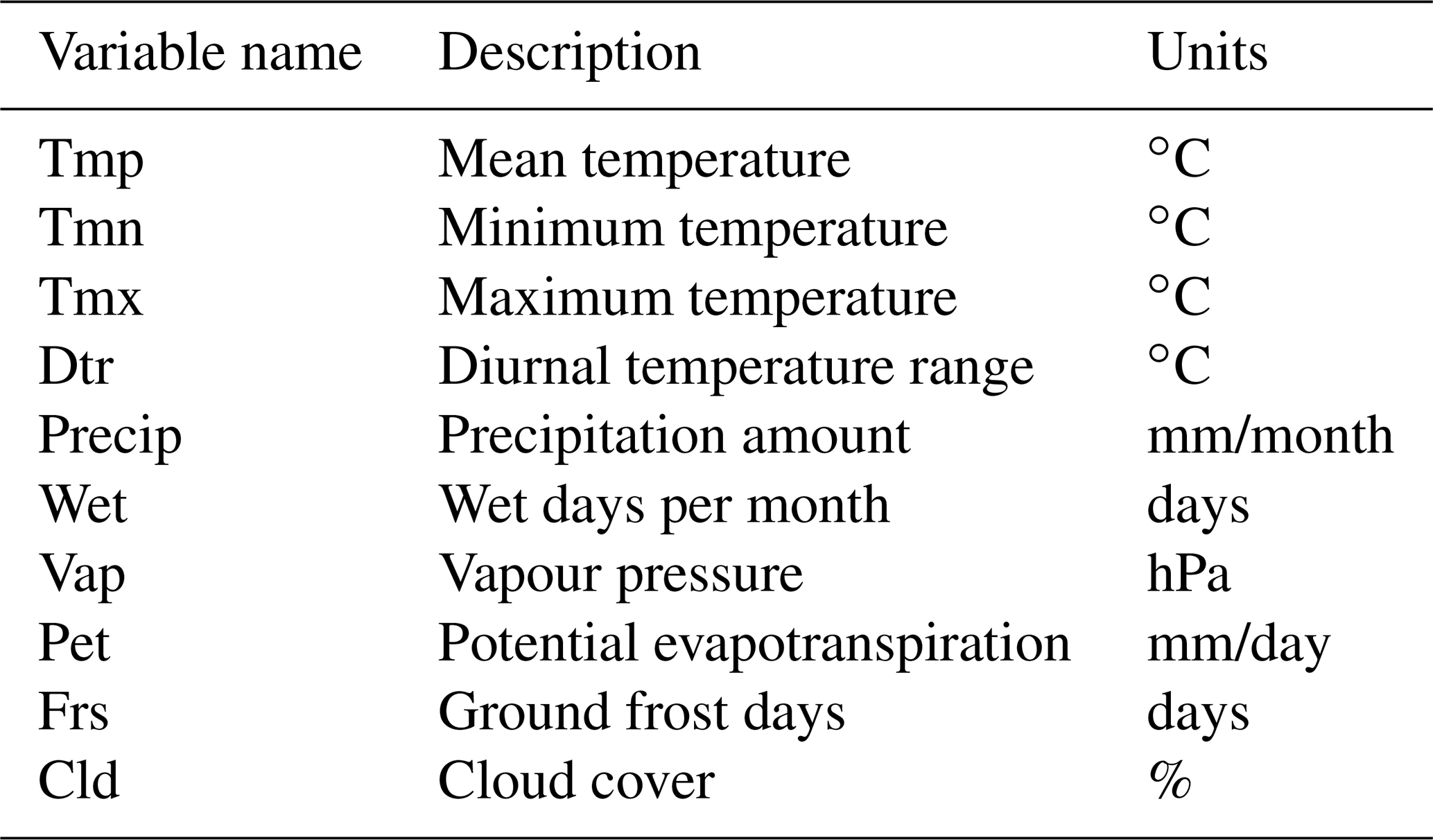
For weather data, we used observed data obtained from the Climate Research Unit (CRU) TS4.04 dataset (Harris et al., 2020). They have global coverage at a resolution of $\mathrm{0.5}{}^{\circ }\times \mathrm{0.5}{}^{\circ }$, cover the period from 1901 to 2019 at a monthly scale and are based on weather station observations. The CRU dataset has a comprehensive range of climatic variables at monthly resolution (Table 1), which makes the dataset suitable for agricultural studies, as shown in Kent et al. (2017), Zhu and Troy (2018), Vogel et al. (2019) and Hamed et al. (2021).

Table 1 Meteorological variables and their descriptions.

Because the analysis involves also the exploration of future scenarios of global warming (GW), we included large ensembles of synthetic weather data produced by the global climate model (GCM) EC-Earth V2.3 (Hazeleger et al., 2012). As a global coupled climate model, it combines atmospheric, ocean, land surface and sea ice models at a resolution of $\mathrm{1.125}{}^{\circ }\times \mathrm{1.125}{}^{\circ }$. We used large ensembles of short-time periods to represent the full range of possible realisations at different levels of global warming (Van der Wiel et al., 2019). Three scenarios are considered: a benchmark representing the present-day climate of 2011–2015 (referred to as PD), a 5-year period representing an average global mean temperature 2 ^∘C above the pre-industrial levels (referred to as 2C) and another 5-year period corresponding to an average of 3 ^∘C above pre-industrial levels (referred to as 3C). To create the large ensembles for each GW scenario, we combined the 5-year periods with 16 different initial conditions and 25 different realisations based on stochastic physics. Together, they culminate in 2000 years of different simulations for each warming level scenario (Fig. C2; see Van der Wiel et al., 2019, for more information on the ensemble setup). Finally, we resampled the large ensembles in 20 members of 100 years to be consistent with the length of the historical dataset (referred to as grouped ensembles hereinafter).

2.2 Data aggregation and detrending

To facilitate the comparison of observed and modelled data, we first upscaled the CRU and crop model data to the same resolution of the EC-Earth data with the first-order conservative remapping method (Jones, 1999). We spatially averaged all data for the region studied (Fig. 2) to focus on the regional scale of weather events and their crop yield impacts, as these have larger influence on global markets. Aggregating data spatially might lead to loss of information, especially on local extreme conditions, but the RF model performance is comparable when running on aggregated data and on all grid points (Table C1).

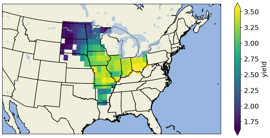
Figure 2 Selected grid points for the main producer states and the mean yields (t/ha) per grid cell as simulated by the EPIC-IIASA model.

The setup of this work relies on comparing large uniform samples at different levels of global warming. Therefore, long-term trends in the data needed to be removed. The yield data from the EPIC-IIASA model have a significant long-term trend, which is a result of the inclusion of atmospheric CO₂ concentration levels in the biomass growth calculation, a process called CO₂ fertilisation (Deryng et al., 2016; Toreti et al., 2020). We regressed the yield data against the global CO₂ concentration levels to remove the long-term trend (Fig. C3). Here, we explore the probability of soybean failure, which is defined by means of a threshold, similarly to Ben-Ari et al. (2018), Vogel et al. (2021), Zhu et al. (2021). Every season with a yield of 1 standard deviation below the mean was considered a failure. The meteorological variables from the CRU dataset were also detrended linearly to remove global warming influence. This way, we isolated the interannual variability component from long-term trends in both meteorological variables and crop yield time series.

2.3 Training and validation of the random forest model

We chose a random forest model to detect failures in soybean yields because of its high performance, flexibility and interpretability. Random forest (Breiman, 2001) is a non-linear and non-parametric statistical model for classification and regression. The model consists of an ensemble of independent decision trees. The decision trees are each trained on random subsamples of the data to provide different predictions, and the final estimate of the model takes into consideration all predictions together, accounting for internal variability. Random forest has become widely popular and is applied in different fields of science. It presents high accuracy while providing low overfitting levels (Breiman, 2001) and is ranked among the best classifiers for real-world problems (Fernández-Delgado et al., 2014).

The first step in designing the random forest model was the feature selection. Among the multiple meteorological variables considered (Table 1), some variables are more relevant than others in predicting crop failures for the region studied. There is also a temporal factor, where the importance of a meteorological variable shows a seasonal cycle. By removing non-relevant variables and months, the data fed to the random forest model are simplified and the model performance possibly increased. We considered multiple feature selection methods because there is no universal method, providing robustness to the selection. The methods are analysis of variance (ANOVA) (Anderson, 2001), mutual information selection (Kraskov et al., 2004), the χ² test and the internal feature selection of the random forest model (Breiman, 2001). At the end of the feature selection step, we obtained the most important meteorological variables to soybean failures.

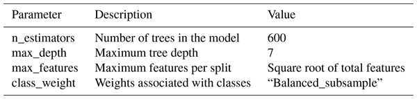
Random forest models require the tuning of internal parameters for an optimal performance. We tuned the random forest's parameters following a resampling technique called cross-validation. It consisted of dividing the data in 10 different splits, where nine splits are used to train the model and the remaining one is used for validation. The process is run 10 times so that every split is used once for testing. In addition, this process was repeated five times with different random divisions, leading to 50 runs in total. The final configuration of the RF parameters can be seen in Table C4. Because the crop yield dataset has less failure seasons than non-failure seasons, the dataset is imbalanced, affecting the model's capacity in identifying the minority class. To address this issue and improve the model performance, we assigned weights to the predictions of each class with values inversely proportional to their frequency. This increases the penalties for underrepresentation of the minority class, balancing the model.

With the RF setup complete, we trained and validated the RF model on the historical data following a $\mathrm{80}/\mathrm{20}$ split, where 80 % of the data were used to train the model and the remaining 20 % were used to validate the model's performance on unseen data. Whilst non-parametric and non-linear models like random forests tend to achieve higher performance than simpler linear models, their complexity renders it more difficult to interpret the outcomes. We included partial dependence plots in the analysis. Partial dependence plots illustrate how model outputs vary according to alterations in one or more inputs, while preserving other inputs values (Friedman, 2001). These plots make the random forest model more interpretable and demonstrate the interactions between meteorological variables and crop yields.

In order to evaluate the random forest performance, we used the Matthews correlation coefficient (MCC) metric on the validation data. It is considered more informative and truthful for the evaluation of binary classification models than other metrics (Chicco and Jurman, 2020). The MCC assesses the performance of the model by quantifying the number of true positives (TPs), the number of true negatives (TNs), the number of false positives (FPs) and the number of false negatives (FNs), as illustrated in Eq. (1). It ranges from −1 to 1, and a score of 0 is equivalent to a random prediction. The model requires both positive data and negative data to be correctly predicted to have a high score, which makes it particularly useful for imbalanced datasets (Chicco and Jurman, 2020). For a comprehensive overview of the model performance, we included additional performance metrics, which are accuracy, precision, recall and F1 score. They can be seen in Appendix A.

$$\begin{array}{}\text{(1)}& \mathrm{MCC}={\displaystyle \frac{\mathrm{TP}\cdot \mathrm{TN}-\mathrm{FP}\cdot \mathrm{FN}}{\sqrt{(\mathrm{TP}+\mathrm{FP})(\mathrm{TP}+\mathrm{FN})(\mathrm{TN}+\mathrm{FP})(\mathrm{TN}+\mathrm{FN})}}}\end{array}$$

We compare the random forest's performance to threshold-conditioned methods, which are frequently used for multivariate risk assessment (Serinaldi, 2016; Salvadori et al., 2016; Zscheischler and Seneviratne, 2017). Two cases are adopted here: the “AND” and the “OR” cases. The “AND” case requires all variables to be equal to or above hazard limits simultaneously for the failure definition. The “OR” case considers at least one of the conditions surpassing the limit to classify as failure (Salvadori et al., 2016). The threshold values for this work were defined as the average conditions of failure seasons in the observed data for each variable minus the corresponding standard deviation of that variables across the sample of failure seasons.

2.4 Exploration of global warming scenarios

To explore soybean failures at different levels of global warming, we used large ensembles of meteorological data from the EC-Earth model. The large ensembles have the advantage of explicitly simulating extreme events that would not be found in smaller datasets due to their rare nature (Van der Wiel et al., 2019). Because the RF model relies on thresholds that may be exceeded more or less frequently in biased climate model data, bias corrections were applied for the analysed regions. We estimated adjustment factors between the detrended CRU dataset between 1916 and 2016 and the PD scenario. Bias adjustment factors were calculated with Detrended Quantile Mapping (Cannon et al., 2015), considering 25 degrees of freedom. The adjustment factors were then applied to the scenarios 2C and 3C, assuming a constant bias (see Fig. C4 for bias correction results for each scenario and Fig. C5 for spatial variability of corrected bias).

To assess the importance of the correlation of the conditions leading to failures, we created permuted versions of each large ensemble by randomly reshuffling the meteorological variables (van den Hurk et al., 2015; Santos et al., 2021), so that the correlation structure between them was removed (referred to as shuffled versions). We also defined a metric called the relative compound contribution. Relative compound contribution measures the importance of the correlation structure between the meteorological variables leading to crop failures. It is a statistical interpretation comparing crop failures under different correlation structures. Relative compound contribution is calculated as the ratio of the failure ratio obtained with the original data to the failure ratio obtained with the shuffled data, $\mathrm{Relative}\mathrm{compound}\mathrm{contribution}=\frac{\mathrm{Failure}{\mathrm{ratio}}_{\mathrm{original}}}{\mathrm{Failure}{\mathrm{ratio}}_{\mathrm{shuffled}}}$. The closer to 1 the relative compound contribution gets, the less important the correlation structure between the variables is. For scenario exploration in this study, we use six scenarios: PD, PD shuffled, 2C, 2C shuffled, 3C and 3C shuffled, each of which was fed into the RF model to obtain the soybean failure probabilities. We assessed the impact of climate change by comparing the failure probabilities for different return periods (calculated as the inverse of the exceedance probability of the specific event to occur) for the PD, 2C and 3C scenarios. Then, we quantified the relative compound contribution by comparing each level of global warming with their shuffled variants. Finally, we compared the RF model with the threshold-conditioned methods to account for differences in the approaches to predict changes with global warming and to quantify the relative compound contribution.

Machine learning algorithms do not extrapolate well for data outside the training range (Hengl et al., 2018). Given the random forest model in this work is trained on historical conditions but applied to GW scenarios, we tested the influence of data outside the training range in the analysis following a three-step test: (1) identify the number of cases outside the training range for each meteorological variable; (2) restrict the values outside the training range to be within the training range; (3) quantify possible differences and inconsistencies in the results between the data before and after the conversion of values outside the training data range (see Appendix B for more information).

2.5 Development of storylines

Storylines were here used to identify the driving components of a historical extreme event and to generate future analogues based on the same event. The 2012 soybean season is our case study, which presented extremely low yields across the main producing regions of the United States. We first verified whether the trained RF model was able to correctly predict 2012 as a failure event and the failure probability assigned to it. To explore the possible analogues of the 2012 season in warmer scenarios, we took two approaches based on the event definition: (1) the first approach was based on the physical conditions that led to the 2012 extreme event, defined here as “event analogues”. We quantified the joint occurrences of meteorological conditions exceeding the 2012 season conditions in the global warming (GW) scenarios; (2) the second approach was based on the impact metric of the event, its yield failure probability estimated by the random forest model, and we defined this approach as “impact analogues” (as, e.g. in Van der Wiel et al., 2019). Using this approach, we quantified the number of seasons in the GW scenarios with equal or higher failure probability predicted by the random forest model. Last, we compared the 2012 season meteorological conditions with the mean meteorological conditions of impact analogues to account for possible changes in the physical aspects of the future analogues.

3 Results

3.1 Feature evaluation and selection

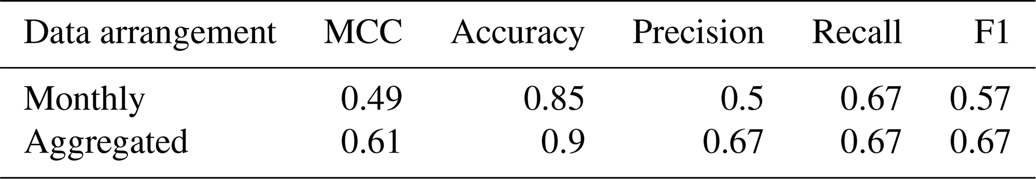
Following the methods section, the first step to build a random forest model is the feature selection. The four feature selection methods (Table C2) show potential evapotranspiration, diurnal temperature range, monthly maximum temperature and precipitation as the most important features. The considered soybean season in the US ranges from May to October, and we see that the months with the highest sensitivity to meteorological conditions are July and August (Fig. C6). The two months correspond to the reproductive phase of soybeans in the region studied (Bastidas et al., 2008; Hatfield et al., 2018), which is a vulnerable crop stage to weather stress (Hatfield et al., 2011; Siebers et al., 2015; Hatfield and Prueger, 2015; Hamed et al., 2021). Based on this, we test an alternative version of the meteorological variables limited to July and August and aggregated along the two months. Results show the aggregated data outperform the monthly data (Table C3). We therefore adopt for this study the aggregated version of the meteorological variables along July and August and compare them to their climatology to identify general features (Fig. 3). Failure years are warmer, have lower levels of precipitation and fewer wet days, larger daily temperature range, higher levels of potential evapotranspiration and lower fractions of cloud cover when compared to the climatology. Vapour pressure and ground frost frequency do not show significant differences between normal and failure seasons, so they are removed from the model training.

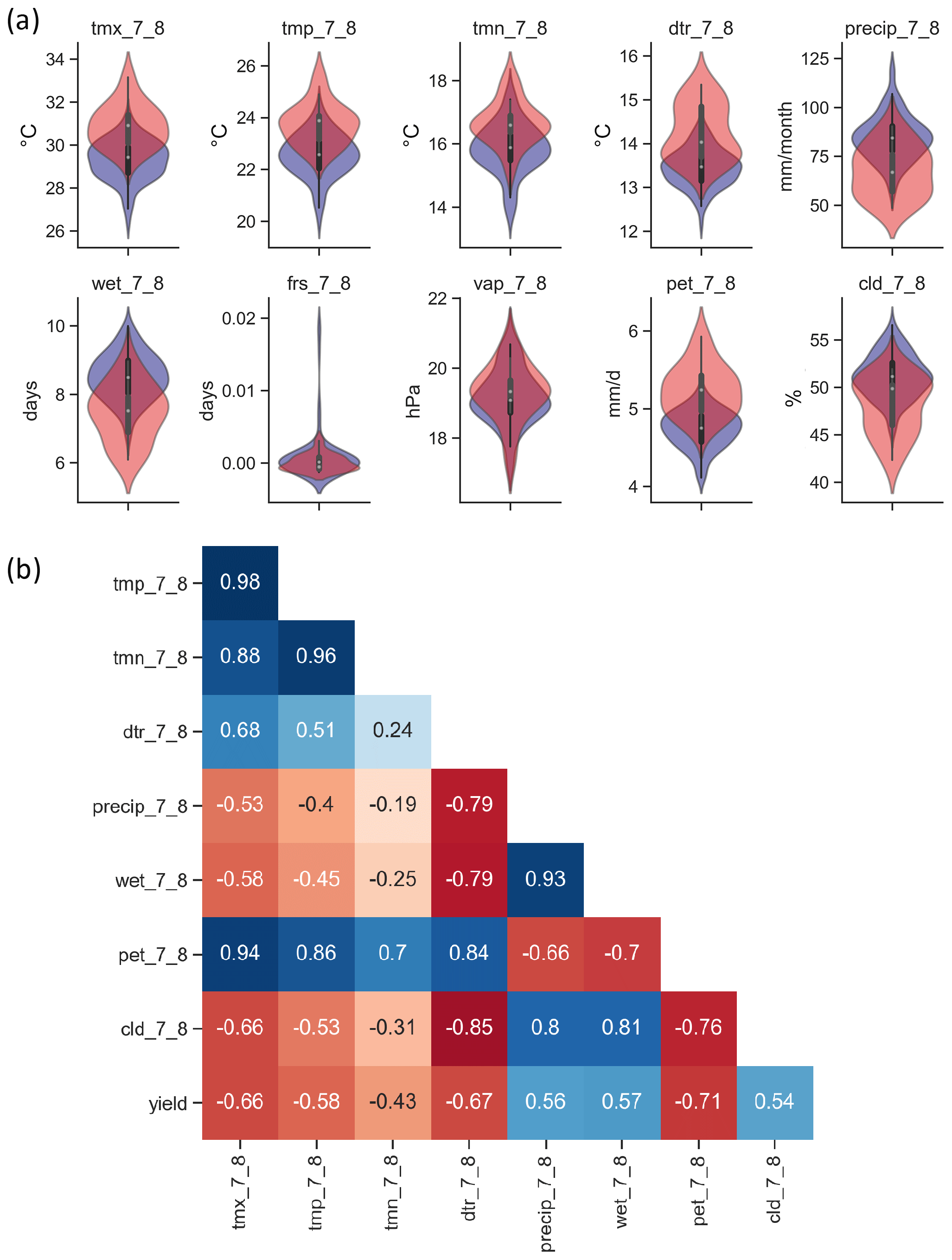
Figure 3 (a) Probability distribution function of monthly values for meteorological conditions of soybean seasons with (red) and without (blue) failures for maximum monthly temperature (tmx), precipitation (precip), diurnal temperature range (dtr), vapour pressure (vap), potential evapotranspiration (pet) and cloud cover (cld). Numbers 7 and 8 indicate the months of July and August, respectively. (b) Pearson's correlation matrix indicating the correlation levels for meteorological variables aggregated along July and August, and crop yields.

The remaining meteorological variables have high correlation levels between themselves, as seen in Fig. 3b. To separate which correlations have statistical redundancy and which have not, we examine each meteorological variable individually. Among the monthly temperature variables, mean (tmp), minimum (tmn) and maximum (tmx) temperature variables are highly interconnected. Tmx shows the best performance among the three variables, so we select tmx as the representative of temperature variables. Monthly precipitation and wet days per month are also highly interconnected, but their performance is similar. As precipitation is a precursor of wet days per month in the CRU dataset (Harris et al., 2020), monthly precipitation is selected. Potential evapotranspiration exhibits high correlation values to all other variables because potential evapotranspiration is derived from temperature, vapour pressure and cloud cover (Harris et al., 2020). Therefore, we consider potential evapotranspiration redundant for this specific experiment. Finally, the three variables selected are maximum monthly temperature, precipitation and diurnal temperature range. They still have considerable levels of correlation, but these have a physical meaning, highlighting the compound nature of meteorological variables leading to crop failures in the region.

3.2 Random forest model evaluation

To evaluate the performance of the random forest (RF) model to link meteorological variables to crop yield failures, we use the Matthews correlation coefficient (MCC) metric (Eq. 1) and compare the results with the “AND” and “OR” threshold-conditioned approaches for reference. The RF model has the highest MCC score at 0.61, while the “AND” approach has 0.54 and the “OR” method only 0.34. The random forest model also performs better than the other methods in the additional metrics as seen in Fig. C7. Therefore, the RF model is successful to link inputs with outputs and outperforms the threshold-conditioned methods.

Partial dependence plots (Fig. 4) explore which variables contribute to successfully distinguish between failure and non-failure conditions. They show the relationships between the meteorological variables' perturbations and crop failure probability. For the selected time period, crop failures are proportional to diurnal temperature range and maximum temperature. Precipitation shows a general inverse proportion to crop failure probability, suggesting low values of precipitation to increase failure probability, as indicated by Fig. 4. Soybean failures in the region studied are thus associated with high levels of monthly maximum temperature, high levels of diurnal temperature range and low levels of precipitation. Furthermore, we observe that the links between crop failures and the meteorological variables are non-linear.

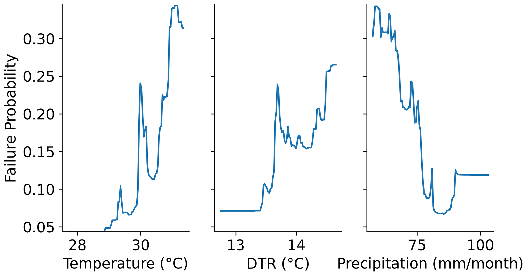
Figure 4 Partial dependence plots showing the failure probability (0 to 1.0) given the variation of the meteorological variables, monthly maximum temperature (temperature), diurnal temperature range and monthly precipitation (precipitation) along the months of July and August.

The random forest model manages to successfully link weather conditions with crop failures, to capture the complexity of the failure, including non-linear relationships, and to outperform the approaches “AND” and “OR”. The success in reproducing crop failure impacts from combinations of weather features for the historical datasets makes the model suitable to explore different climate scenarios.

3.3 Scenario exploration

The trained and validated random forest model is applied to the grouped ensembles to estimate crop failure probabilities for different global warming scenarios. First, we determine if the crop failure probabilities obtained for the present-day (PD) scenario is consistent with the historical data from EPIC-IIASA (Fig. 5a). The width of the grouped ensemble (shading) indicates the many possible manifestations due to natural variability. The observed data are just a single realisation over that period, and we see the observed data are within the range of the ensemble. For the estimation of global warming influence on crop failure probabilities, we quantify the return periods of failure probabilities for the PD, 2C and 3C scenarios (Fig. 5b). The 2C scenario shows increased failure probabilities for any given return period with respect to the PD scenario, while the 3C scenario shows slightly higher failure probabilities than the 2C scenario. Global warming is therefore likely to increase the occurrence of soybean failures, but the difference between 2C and 3C is not significant.

Figure 5 (a) Random forest model failure probabilities for different return periods, comparing observed data (black) to the PD scenario (blue). (b) Return periods for PD (blue), 2C (orange) and 3C (pink). Dots show the 20-member mean; shading shows the range across the 20 members. The dashed line represents the failure probability of the 2012 season predicted by the RF model (Sect. 3.4).

The relative compound contribution is quantified by considering two versions of data arrangement: original (ordered) and shuffled (unordered, no correlation between variables). Figure 6 presents the crop failure probabilities for different return periods. In all scenarios, the return periods for the 0.5 failure probability threshold are shorter for the original data than for the shuffled data. Thus, the combination of the meteorological variables is relevant for the failure likelihood of soybeans (e.g. low precipitation concurs with above average temperatures), which highlights the compound nature of the crop failure drivers. For the 2000 years of data in each scenario, the RF model predicts 276 failure seasons for the PD original data, whereas the shuffled version has 63 failure seasons predicted. The failure seasons for the 2C original and shuffled data are, respectively, 616 and 241 seasons, and for the 3C scenario, 621 and 353 seasons. Thus, while the number of failure seasons increases with global warming for the original data, the increase in the number of failure seasons for the shuffled data is larger. A reduction in the relative compound contribution for the 2C and 3C scenarios suggests the correlation structure between meteorological variables becomes less relevant for our definition of crop failure.

Figure 6 Random forest model failure probabilities for different return periods, based on original data (variable correlations as normal, blue) and shuffled data (variable correlation removed, orange) for three climatic periods: (a) present-day, (b) pre-industrial +2C warming and (c) pre-industrial +3C warming. Dots show the 20-member mean; shading shows the envelope of variability for the grouped ensemble.

We demonstrate the changes in the physical conditions for failure and non-failure seasons at each scenario (Fig. 7 for 3C and Fig. C8 for 2C). Median temperature values along July and August of failure years increase by 1.1 ^∘C for 2C and 2.6 ^∘C for 3C. Median precipitation values of failure years show little change, slightly increasing by 2.4 mm/month for 2C and 0.18 mm/month for the 3C compared to PD. Median diurnal temperature range values of failure years show a slight decrease of 0.33 and 0.36 ^∘C for 2C and 3C scenarios, respectively. Despite median values of precipitation not changing significantly, we see an increase in the failure rate at the low end of the rainfall distribution for 2C and 3C (Fig. 7a top). Together with temperature extremes, the results suggest more frequent and intense joint warm and dry conditions in the future (Fig. 7a). However, we see also an increase in the failure distribution at higher (and thus less critical) precipitation levels for both 2C and 3C than for PD. A similar pattern is observed for the diurnal temperature range values, where less critical levels of DTR still incur failures (Fig. 7b). Extreme temperature values dominate the failure probability at warmer levels, which reduces the need for other variables to be extreme as well to generate failures. Therefore, the univariate increase in the temperature values due to global warming is associated with the increase of soybean failure ratios and with the decrease of the relative compound contribution.

Figure 7 Kernel density estimate plots for seasons with and without failures at different GW scenarios: (a) for maximum monthly temperature and precipitation and (b) temperature and diurnal temperature range.

We compare the RF model with the “AND” and “OR” approaches to account for differences in the approaches in quantifying the relative compound contribution and the predicted changes with global warming. The “AND” approach shows the lowest ratio of failure for both original and shuffled data (Fig. 8a) but also the highest levels of relative compound contribution (the difference between ordered and permuted datasets, Fig. 8b). The “OR” approach only requires one critical variable for failure definition, which implies the highest failure ratios (Fig. 8a). Moreover, breaking the correlation structure and shuffling the meteorological variables for this approach means increasing the number of failure seasons, which implies relative compound contribution has a decreasing role. Finally, the random forest model predicts an intermediate number of failure seasons. The RF model suggests relative compound contribution as an enhancing factor for crop failures (in contrast to the “OR” method) but not as much as suggested by the “AND” model (Fig. 8a). Because the RF model presented the highest performance scores previously, we consider it to be the most reliable in quantifying relative compound contribution, while the others either underestimate or overestimate the importance of compound structure for crop failures. Nevertheless, all three methods agree that relative compound contribution loses importance under warmer scenarios, trending towards a level of 1.0 (no relative compound contribution, Fig. 8b).

Figure 8 (a) The failure ratios for ordered and shuffled PD data for the three approaches: AND, OR and RF with respect to the failure ratio of observed data; (b) relative compound contribution level (original failure ratio divided by shuffled failure ratio) of each approach for the GW scenarios.

The extrapolation test indicates all three meteorological variables in the climate projections have values outside the training range, with temperature extremes exceeding the historical range as the most frequent case of extrapolation. However, the conversion of values outside the training range into values within the training range does not change the results obtained. This is because the model is a binary classifier, and the failure is defined within the historical data. Unprecedented extreme values do not change the failure definition, as it follows the assumption that values outside the training range are similar to the extremes in the training range (see Appendix B for further information). With the extrapolation test demonstrating that values outside the training range do not affect the results, the impacts of different levels of climate change on soybean failure probability in the region are validated. Next, we investigate if these general conclusions also hold for specific cases like the extreme 2012 season using a storyline approach.

3.4 Storyline analysis: the 2012 season and future analogues

The year 2012 had an extreme loss in US soybean production, with exceptionally low yields in the majority of the producing region (Fig. 9a). We test the random forest model for the 2012 season to identify the meteorological variables associated with the failure event. The season stood out as all three selected meteorological variables presented extreme values (Fig. 9b), with precipitation approximately at −2 SD (standard deviations), temperature above 2 SD and DTR scoring the highest recorded value exceeding 3 SD. When used to predict the probability of crop failure due to the meteorological conditions described above, the RF model indicates a 0.96 likelihood of the 2012 season to be a failure.

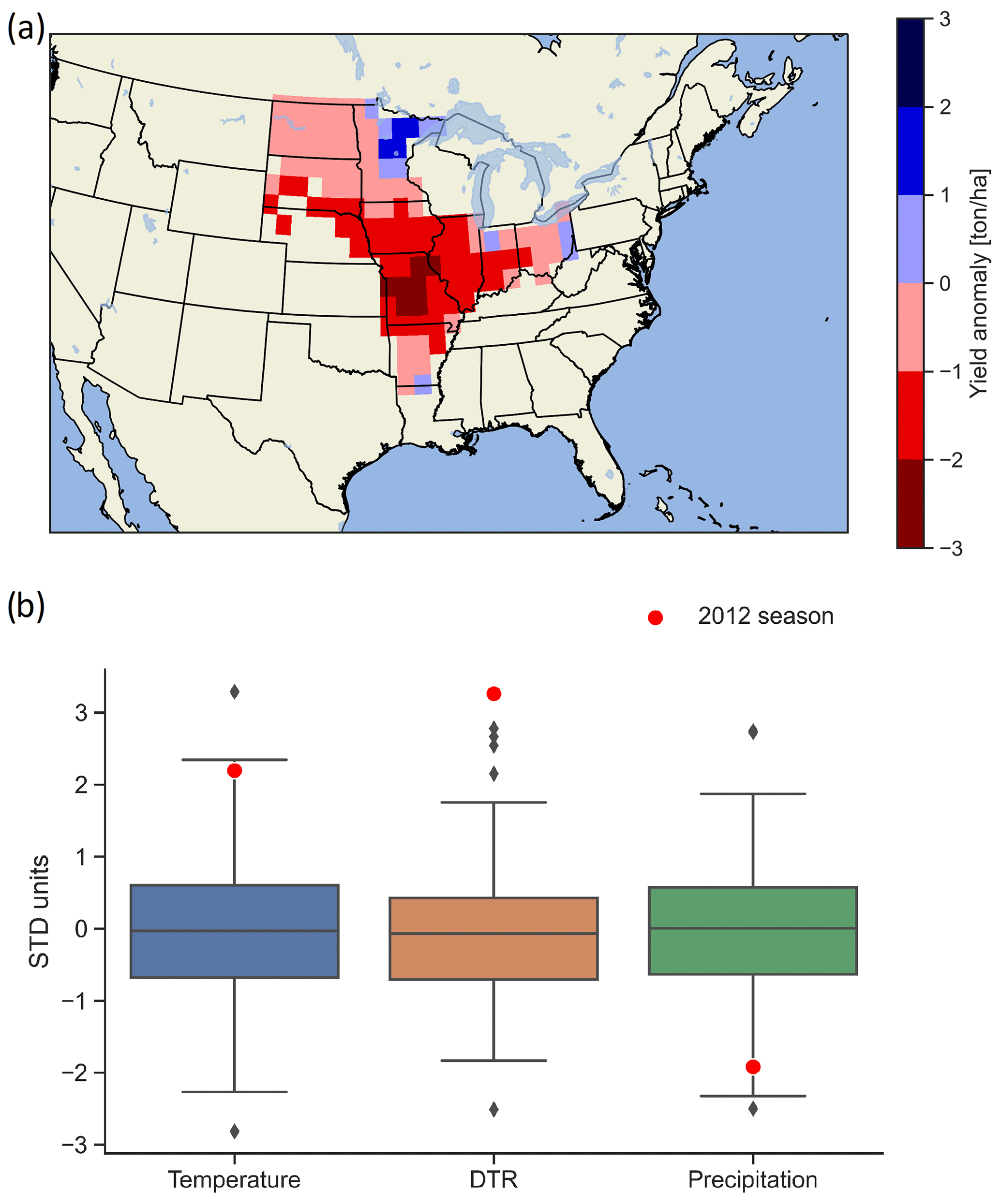
Figure 9 (a) Map of the yield anomaly for the 2012 season compared to the averaged historical yield data from EPIC-IIASA. (b) Normalised meteorological variables for the observed dataset and the corresponding 2012 season climatic conditions.

We create 2012 season analogues using both impact and event perspectives. Event analogues are defined as the joint occurrences of the 2012 climatic conditions (as in Fig. 9b), while impact analogues are defined as the number of seasons with failure probability assigned by the random forest model as equal or higher than the probability of the 2012 season (i.e. probability >=0.96). The event analogues have a occurrence ratio of 0.0015 (three events in 2000 years, 666-year return period) for both PD and 2C scenarios, but it is not seen in the 3C scenario (Fig. C9), suggesting a highly rare event that does not increase with global warming. However, we find a higher ratio of 2012 impact analogues for the PD scenario, 0.022 (44-year return period), 14 times the PD event analogues. Impact analogues also increase in frequency at warmer scenarios, 0.038 (26-year return period) for 2C and 0.042 (24-year return period) for 3C. The difference in results between the two types of analogues is mainly due to the DTR values, illustrated by Fig. 10a–c, which show the ratio of exceedance (the frequency of seasons exceeding a given threshold) of the 2012 meteorological conditions for each variable individually. Event analogues require all variables to exceed the corresponding 2012 conditions. While we observe an increase in the number of seasons with temperature and precipitation exceeding the 2012 conditions in global warming scenarios, DTR does not increase with GW. Therefore, DTR becomes a bottleneck in the generation of event analogues. Impact analogues, on the other hand, are predicted to increase with global warming because they are defined based on the impact metric (failure probability) and bypass the DTR limitation. In addition, by relying on the impact metric, the meteorological conditions of the analogues can be analysed for changes due to global warming (Fig. 10d–f and C10). The impact analogues of the year 2012 show warmer temperatures during summer with respect to the original event. For precipitation, the analogues are significantly drier than those in the year 2012 during July and August, the months in which the RF model takes into account. Finally, the analogues present lower DTR values during most of the year.

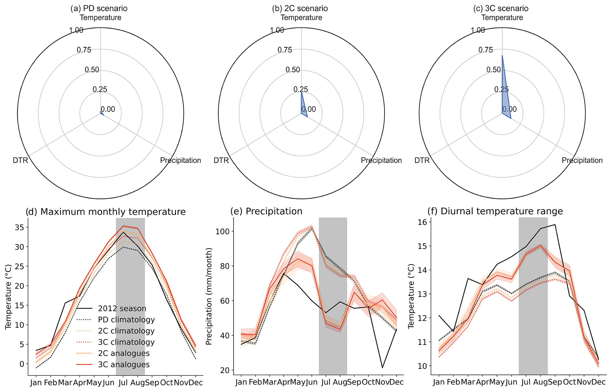
Figure 10 Radar graphs showing the number of seasons exceeding the 2012 values for each meteorological variable for present-day (a), 2 ^∘C global warming scenario (b) and 3 ^∘C global warming scenario (c) scenarios. Annual cycle of the historical years, the 2012 season, the impact analogues and their corresponding climatology for maximum monthly temperature (d), precipitation (e) and diurnal temperature range (f). Coloured shadings represent the 95 % confidence interval for each scenario. The vertical grey bar represents the months considered in the training of the RF model.

4 Discussion

A large portion of crop failures is attributed to combinations of meteorological drivers (Zampieri et al., 2017; Zscheischler et al., 2017) and the interactions between weather and crops are known to be non-linear (Schlenker and Roberts, 2009; Zscheischler et al., 2017). It is a challenge, therefore, to identify the variety of combinations of weather conditions that can lead to crop failures. We argue that a model explicitly designed based on the impact, here crop failure, allows the conversion of a multivariate problem into a univariate variable, which simplifies the analysis, and improves the quality of results (van der Wiel et al., 2020). The random forest model here developed is successful at predicting soybean failure seasons and shows an overall better performance than benchmark methods. It adds to the list of works that demonstrate the usefulness of impact-inspired approaches (Ben-Ari et al., 2018; Vogel et al., 2021; van der Wiel et al., 2020; Hamed et al., 2021; Zhu et al., 2021). The feature selection process used here combines machine learning with findings from the literature to identify compound drivers of soybean failures in the US. Temperature, precipitation and diurnal temperature range along July and August are deemed key climatic drivers in the region studied. The meteorological variables identified in this work are in agreement with the work of Vogel et al. (2021), which also shows temperature, precipitation and DTR to be important meteorological variables for crop development, and with the work of Hamed et al. (2021), which highlights the harmful combination of hot and dry conditions along summer for soybeans in the same region. This work considers only meteorological variables during the growing season of rainfed soybeans, so management practices, irrigation and subsurface conditions are not considered. The meteorological variables are at a monthly scale, which has been used in past studies as well (Ben-Ari et al., 2018; Vogel et al., 2019; Hamed et al., 2021). However, adopting shorter timescales could lead to additional information on how weather interacts with crops. We spatially aggregate the climate and crop data over the region analysed to focus on crop failures and meteorological conditions at the regional scale. While this approach allows us to analyse the main dynamics of the region, information on local extreme conditions is not attained. Another caveat is that we do not account for CO₂ concentrations, due to our focus on year to year variability. Yet, CO₂ fertilisation is an important factor when considering crop–climate interactions and when looking at the effects of future climate change (Schlenker and Roberts, 2009; Deryng et al., 2016; Toreti et al., 2020).

Even though extrapolation with statistical models carries risks (Hengl et al., 2018), there are works that train statistical models on historical data and apply them on global warming scenarios (Schlenker and Roberts, 2009; Roberts et al., 2017; Crane-Droesch, 2018; Zhu et al., 2021). The random forest model used here is a classifier trained to detect a class of failure events determined by the historical dataset. The decision trees within the random forest are threshold based, so values outside the training range are categorised together with historical extremes. Furthermore, the purpose of the work is to measure the frequency of historical failures and analogues under future conditions, instead of quantifying the magnitude of failures under unprecedented extreme conditions. Finally, we run a extrapolation test and results show no influence of values outside the training data range in the results (Appendix B). Together, these factors validate the application of the random forest model for global warming scenarios under these assumptions.

We use three large ensembles with different levels of global mean surface temperature to investigate the influence of climate change on crop failure probabilities. Soybean failures increase in frequency for both 2 and 3 ^∘C warmer worlds. When compared to the literature, some works support future global warming negatively affecting soybeans in the Unites States (Schlenker and Roberts, 2009; Deryng et al., 2014; Schauberger et al., 2017; Zhao et al., 2017), while others indicate that soybeans in the same region could actually benefit from climate change due to an intensification of local rainfall (Lesk et al., 2020). In the EC-Earth runs, we see a drying trend for extreme years in the midwestern United States (Fig. 10d), which explains the different results. Dynamical aspects of global warming have large uncertainties due to high internal variability (Fischer et al., 2014), and the ensemble of CMIP6 models does not show significant changes for the months of July and August in the region studied (Almazroui et al., 2021). The adoption of different global climate models and the evaluation of climate change impacts conditioned on storylines of different levels of precipitation are alternatives that could explain the discrepancies seen above and should be further explored in the future. Furthermore, we do not consider potential adaptation measures by farmers such as the expansion of irrigation systems to counteract any possible drying trends.

Our results show climate change is expected to impact both univariate and multivariate components of crop failure. From a univariate perspective, temperature is expected to increase significantly, contributing to more frequent failures. In a warmer world, the same levels of precipitation lead to higher rates of crop failures than under the current climate conditions. The DTR projections indicate a descending trend, which in itself reduces crop failure probability according to our model. DTR is highly relevant for crop development, with previous studies showing the multiple impacts it can have on crops (Lobell, 2007; Zhang et al., 2013; Chen et al., 2015; Verón et al., 2015; Hernandez-Barrera et al., 2017; Rahman et al., 2017; van Etten et al., 2019). High values of DTR suggest peaks in high daytime temperature, which can disrupt the photosynthetic activity of crops (Allakhverdiev et al., 2008). High values of DTR can also indicate low nighttime temperatures or night frosts, with capacity to damage crops during all stages of crop growth (Barlow et al., 2015). A study based on EPIC to simulate maize yields in the US has demonstrated that higher DTR values lead to greater evapotranspiration losses, reducing the yield outputs (Dhakhwa and Campbell, 1998). On the other hand, low values of DTR could indicate low solar radiation or high cloud coverage, both harmful for crops (van Etten et al., 2019; Vogel et al., 2019; Lobell, 2007). The decrease in DTR values due to global warming is mainly associated with a higher increase of minimum nighttime temperature than daytime temperature (Qu et al., 2014; Sun et al., 2019). From a multivariate perspective, the correlation structure of the variables contributes to the occurrence of compound events, as previously shown by (van den Hurk et al., 2015) and (Santos et al., 2021). Yet, we observe a decrease in its importance under global warming conditions for the failure yield threshold adopted here (Fig. 6). A higher frequency of years with critical temperature during summer makes crop failures mostly dependent on precipitation values. Therefore, while still physically a compound event, the soybean failures under global warming become statistically similar to a univariate event based mostly on precipitation.

The random forest model defines the year 2012 as a highly likely failure season. That year, the climatic conditions during the reproductive phase of the crop were dry and hot, and had a particularly high diurnal temperature range. When considering the event analogues, i.e. looking at the event given its meteorological specifics, results show the 2012 season to be particularly rare and unlikely to increase in frequency due to climate change in the projections considered herein. Yet, when assessing the impact analogues, defined as the likelihood of events with a similar failure probability using the random forest model, more events are identified in the PD scenario compared to the event analogues. Furthermore, we find that significant increases are predicted for warmer scenarios. The differences between event analogues and impact analogues reflect the concept behind each approach. Event analogues are based on the physical conditions of the event and obtained by quantifying the joint occurrence of these conditions in the ensembles. Impact analogues, on the other hand, are based on the impact metric, accounting for all combinations of weather that lead to the same failure probability of the 2012 season. This difference between an event-based and impact-based approach was also highlighted by (van der Wiel et al., 2020). In spite of the exceptionally high DTR value for the 2012 season, the GW scenarios show decreasing DTR values with respect to the mean temperature increase. This evidence is supported by the literature, suggesting DTR is inversely proportional to global warming (Qu et al., 2014; Sun et al., 2019). Lower DTR values therefore constrain the increase of 2012 event analogues, even though the other two meteorological variables show a significant increase. Since the random forest is able to explicitly account for the impact of the 2012 season, it detects other possible combinations of meteorological variables leading to 2012 impact analogues. Furthermore, impact analogues of the 2012 season in the future display a change in their physical properties: they are hotter and drier but with lower values of diurnal temperature range. Results highlight the importance of the inclusion of impact analogues in storylines creation. Storylines have been commonly used to generate counterfactuals by reproducing similar physical events to historical ones, adopting an event-inspired perspective (Shepherd, 2019; Sillmann et al., 2020). However, storyline counterfactuals (Shepherd et al., 2018) could profit from also explicitly considering the impact perspective, as we have shown with the impact analogues created with the random forest model to directly model crop failures. The inclusion of the impact perspective into storylines allows for a more comprehensive view of future realisations when compared to considering only the occurrence of similar physical events. Note that for society it is the impacts that matter, rather than the meteorological condition. Furthermore, using impact analogues allows for the estimation of possible changes in the physical characteristics of analogues due to global warming, increasing the robustness of climate risk assessment for future scenarios.

5 Conclusions

This work presents an evaluation of the impacts of global warming on weather-induced soybean failure events. Its novelty lies in combining a statistical model capable of simulating non-linear and compound interactions, the random forest model, with large ensembles of future global warming scenarios. The steps to create the model are the selection of the most important meteorological variables during the growing phase of the crop and the training of the model on historical data. We explore the influence of global warming on soybean crop failure with the use of large ensembles at different levels of global warming. The model is successful at identifying failure seasons in the historical data and selecting the most relevant meteorological variables for crop failures. When compared to two benchmark methods, the model presents an overall better performance.

The main findings of the paper suggest soybean failures in the midwestern United States are likely to increase with global warming mainly due to warmer atmospheric conditions during summer. With more frequent warmer years, the joint hot–dry conditions leading to crop failures become more common. Conversely, the increase in frequency of warmer years renders the occurrence of joint hot–dry extremes more dependent on summer precipitation anomalies, reducing the importance of the relative compound contribution. With global warming, the crop failures approximate statistically to a more univariate behaviour, despite still being physically the results of compound events. Estimations of future analogues of the 2012 season diverge according to the approach used. If considering the event-inspired threshold-conditioned method, event analogues are deemed extremely rare and do not increase in likelihood with global warming. However, when using the impact-inspired model here developed, we show that impact analogues are actually more common than what was originally predicted by the threshold-conditioned method, and the number of analogues is expected to significantly increase with warmer climates. Moreover, we observe changes in the physical properties of the impact analogues under global warming, becoming warmer and drier, but with lower diurnal temperature range levels. Impact analogues complement event analogues, improving the risk estimation of storylines.

Appendix A: Additional performance metrics

To provide robustness to the performance analysis, additional performance metrics were used to evaluate the model. Accuracy quantifies the amount of TPs and TNs out of the total data (that is, the true data plus FPs and FNs (Eq. A1). Precision defines the fraction of TP cases out of the total predicted positive cases by the model (Eq. A2). Recall measures the correct fraction of positive cases out of the true positive cases (Eq. A3). The F1 score is a metric used to address false positives and negatives (Eq. A4).

$$\begin{array}{}\text{(A1)}& {\displaystyle }\mathrm{Accuracy}={\displaystyle \frac{\mathrm{TP}+\mathrm{TN}}{\mathrm{TP}+\mathrm{TN}+\mathrm{FP}+\mathrm{FN}}}\text{(A2)}& {\displaystyle }\mathrm{Precision}={\displaystyle \frac{\mathrm{TP}}{\mathrm{TP}+\mathrm{FP}}}\text{(A3)}& {\displaystyle }\mathrm{Recall}={\displaystyle \frac{\mathrm{TP}}{\mathrm{TP}+\mathrm{FN}}}\text{(A4)}& {\displaystyle }\mathrm{F}\mathrm{1}={\displaystyle \frac{\mathrm{2}\mathrm{TP}}{\mathrm{2}\mathrm{TP}+\mathrm{FP}+\mathrm{FN}}}\end{array}$$

Appendix B: Extrapolation test

Machine learning algorithms have the drawback of not extrapolating well for data outside the training range. However, there are works that use the extrapolation technique to predict crop impacts under global warming scenarios with statistical models (Schlenker and Roberts, 2009). Yet, the setup of the experiment is to quantify the number of failure events in global warming scenarios based on failures already identified in the historical data. The presence of values outside the training data range might not affect the random forest model, because the same failure probabilities are assigned to these values as to the closest values in the training range (corresponding maximum and minimum values). This is due to the decision trees that compose the random forest. The decision trees divide the input space using thresholds, which group similar input values together. Values outside the training data are grouped together with the corresponding extreme values within the training data, because they are within the same input space according to the decision tree (lower or higher than a threshold value). We verify the validity of the experiment with an extrapolation test based on three steps: (1) identify the number of cases outside the training range for each meteorological variable; (2) convert the values outside the training range into the closest values within the training range; (3) quantify differences and inconsistencies in the results between the GW scenarios before and after the conversion.

Table B1 Number of years with values above the historical maximum (“above”) and below the historical minimum (“below”) for each of the GW scenarios (PD, 2C and 3C). Each scenario has 2000 years in total.

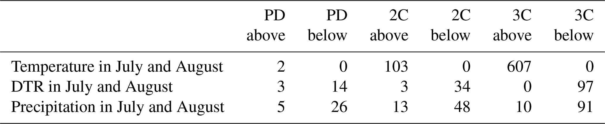
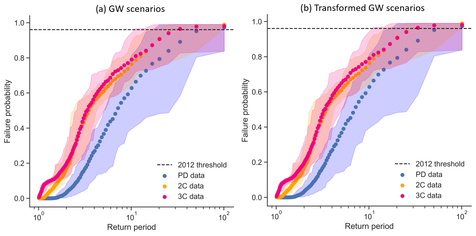
Figure B1 (a) Random forest model failure probabilities for PD (blue), 2C (orange) and 3C (pink); panel (b) is the same as (a) but for values adjusted to the training data limits. Dots show the 20-member mean; shading shows the range across the 20 members. The dashed line represents the failure probability of the 2012 season predicted by the RF.

The number of events in each GW scenario that is outside the training range is shown in Table B1. After the conversion of values outside the training data range into values within the training data range, the results stayed the same for all scenarios (Fig. B1). We assume the presence of values outside the training range does not influence the results obtained with the random forest model.

Appendix C: Additional figures

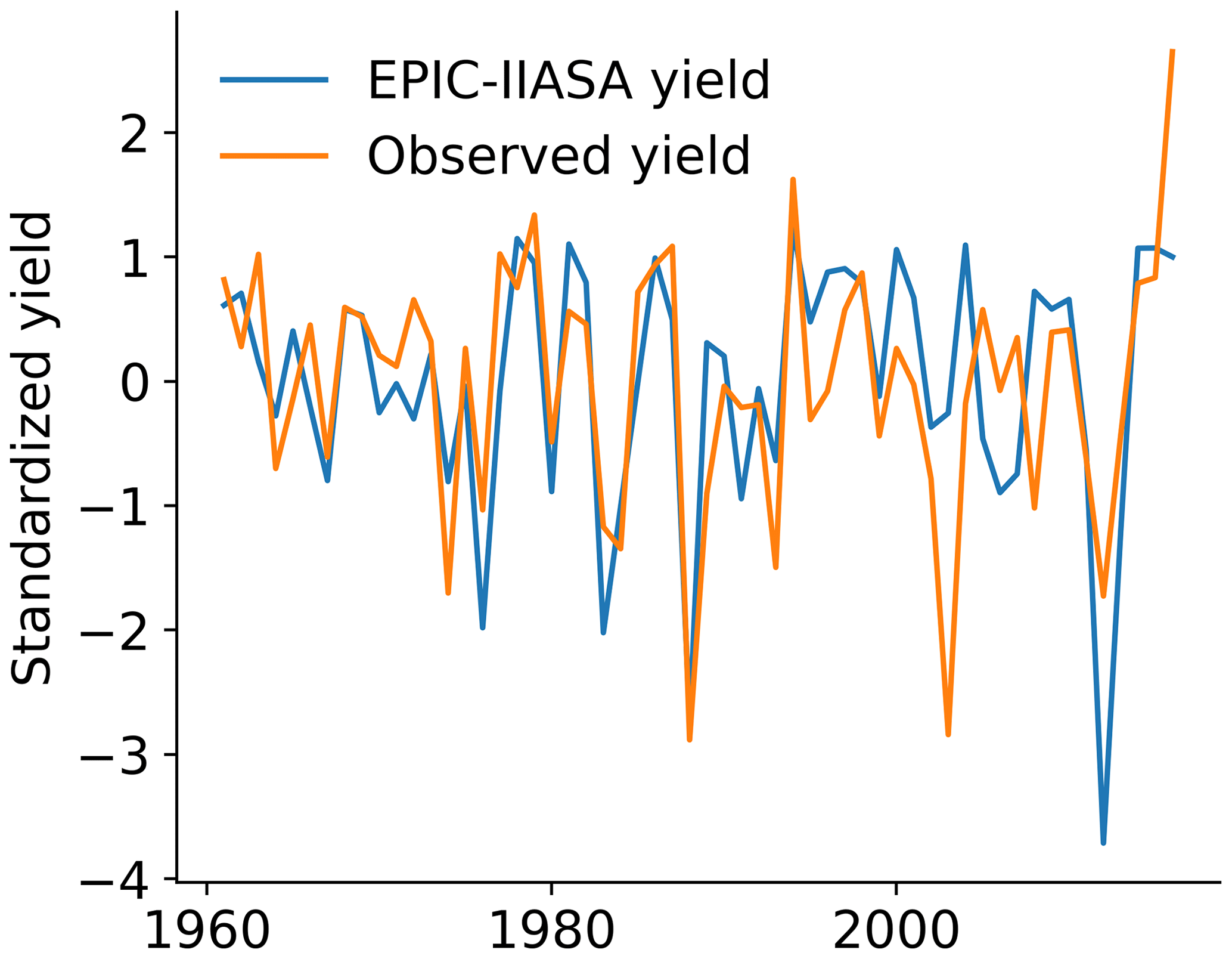
Figure C1 Standardised comparison between the EPIC-IIASA simulated yields and the observed yield dataset of the USDA (United States Department of Agriculture) for the region considered in this work.

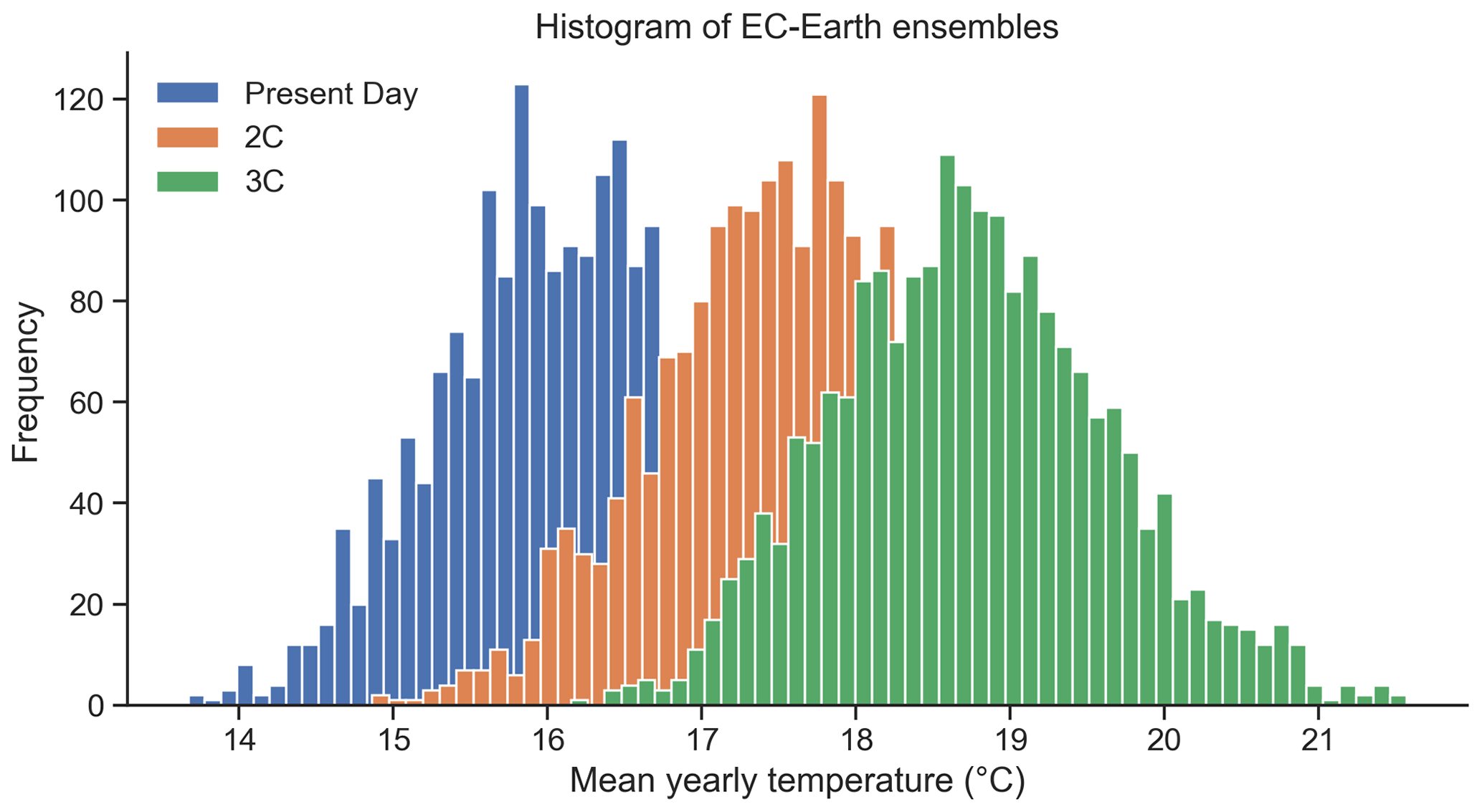
Figure C2 The distribution of mean yearly temperatures in the midwestern United States of EC-Earth ensembles for the present-day scenario (blue), 2 ^∘C global warming scenario (2C, orange) and 3 ^∘C global warming scenario (3C, green) scenarios.

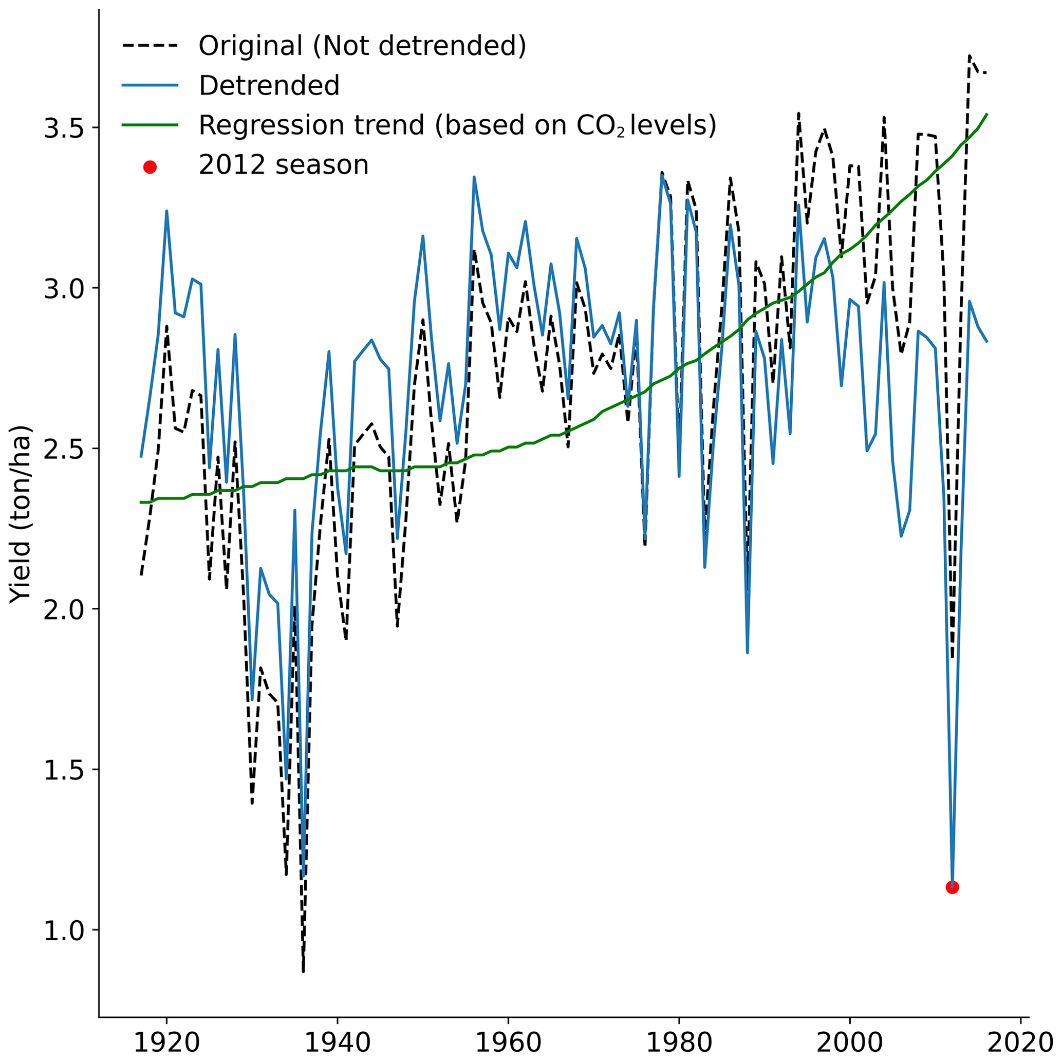
Figure C3 Time series of averaged US soybean yields for the selected area (dotted black line) and its detrended counterpart (blue). The 2012 season is highlighted in red. The regression trend based on the global CO₂ levels that is used to detrend the soybean yields is shown in green.

Figure C4 Mean annual cycle for the selected variables: temperature (a, b, c), DTR (d, e, f) and precipitation (g, h, i). Panels (a), (d), (g) presents the observed data (black), the original EC-Earth PD data (blue) and the EC-Earth after bias correction (dashed red). In panels (b), (e), (h) and (c), (f), (i) the bias-corrected EC-Earth data for the present-day scenario (PD, dashed red) is then compared with the bias-corrected versions of the 2 ^∘C (2C, b, e, h, orange) and 3 ^∘C (3C, c, f, i, green) scenarios.

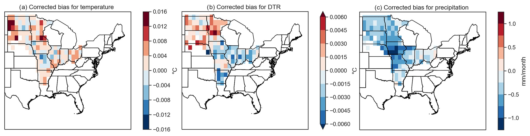
Figure C5 Spatial variability of bias-corrected values between observed data and EC-Earth PD scenario for (a) monthly temperature values, (b) DTR and (c) precipitation.

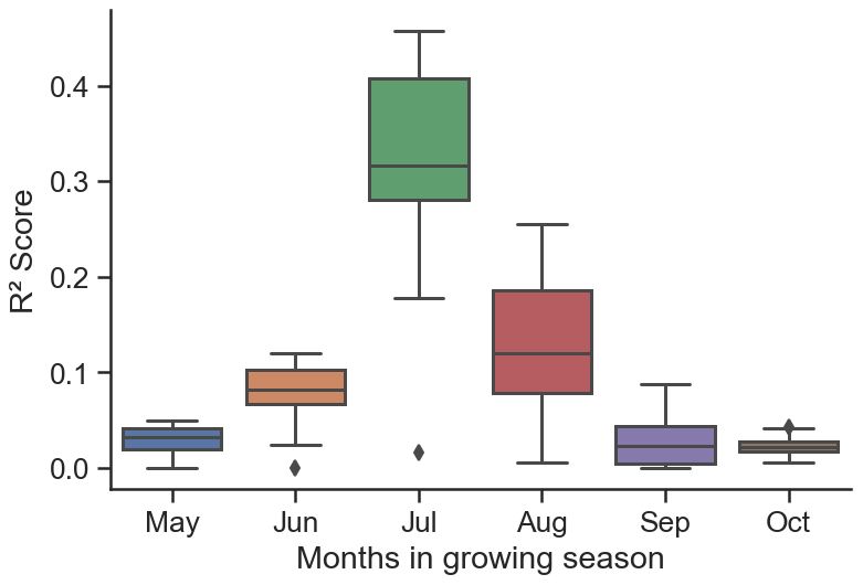
Figure C6 Coefficient of determination between soybean yields and all meteorological variables considered in this study grouped by month of the growing season.

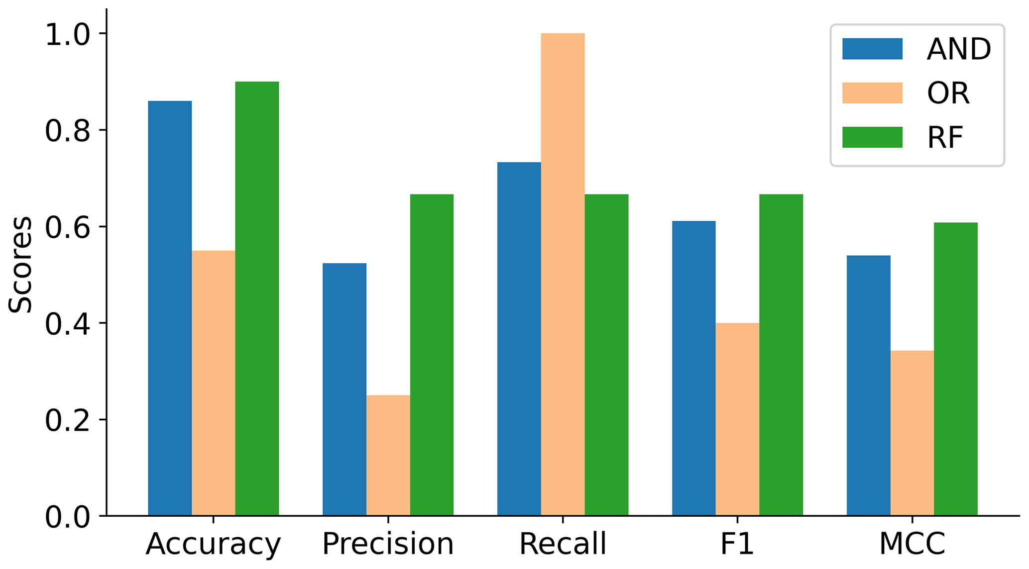
Figure C7 Evaluation of each approach in identifying crop failures for the observed data under different performance categories: accuracy, precision, recall, F1 and MCC. The approaches are AND (blue), OR (orange) and RF (green).

Figure C8 Same as Fig. 7 but for the 2C scenario.

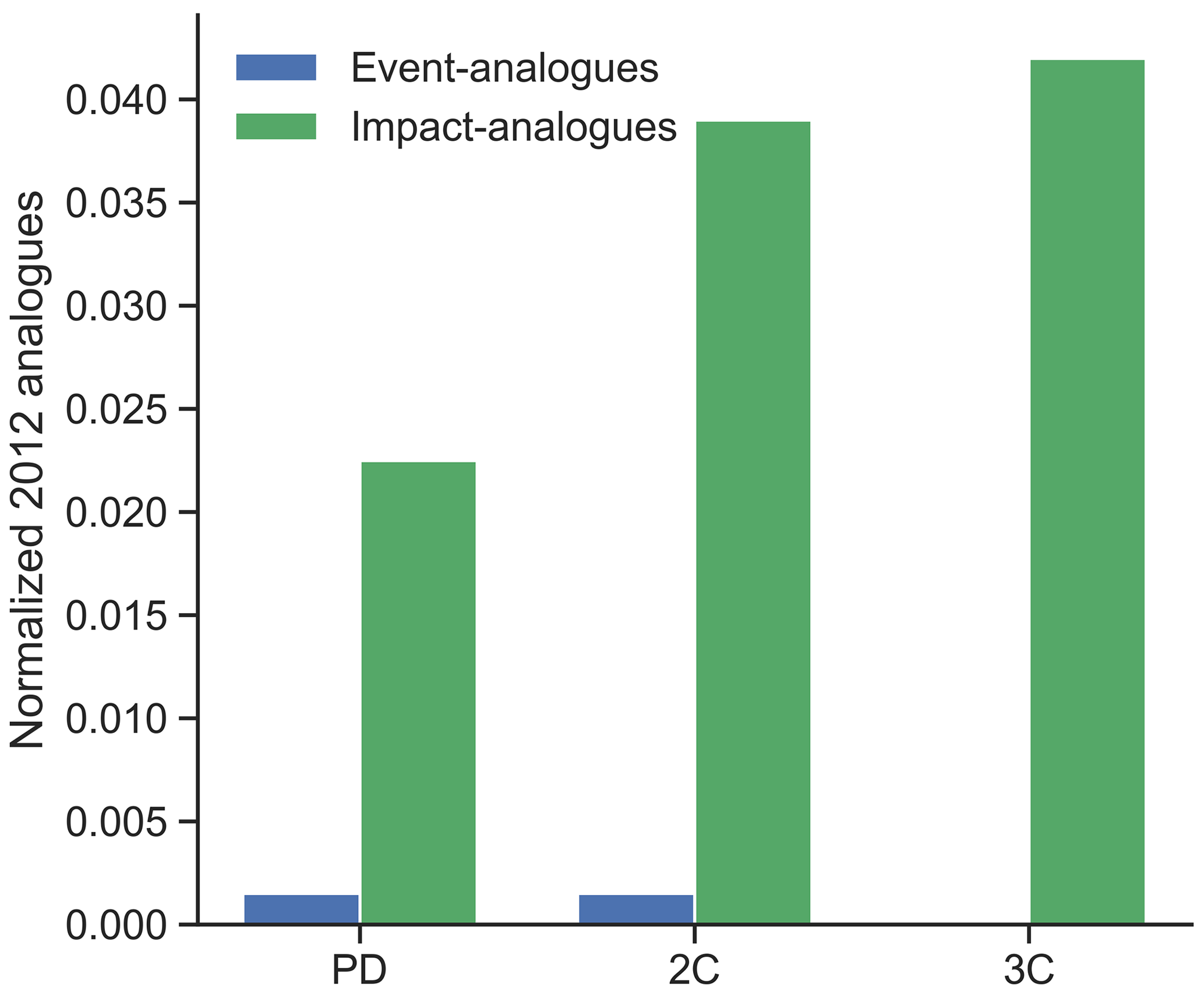
Figure C9 Event analogues (blue) and impact analogues (green) of the 2012 season for each GW scenario: present-day (PD), 2 ^∘C (2C) and 3 ^∘C (3C) scenarios.

Figure C10 Same as Fig. 7 but for the 2012 impact analogues.

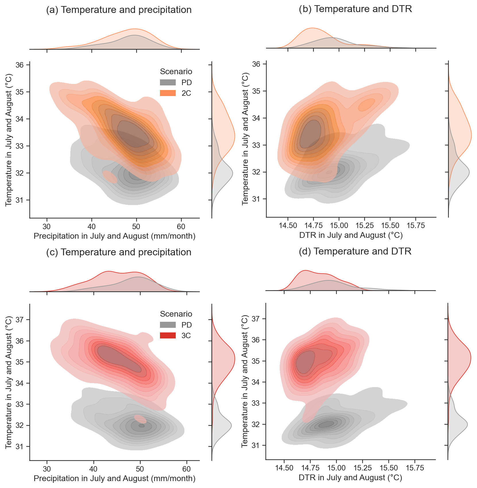
Table C1 Comparison of the random forest model performance between spatially aggregated data over the region studied and the gridded spatial format, considering all grid points.

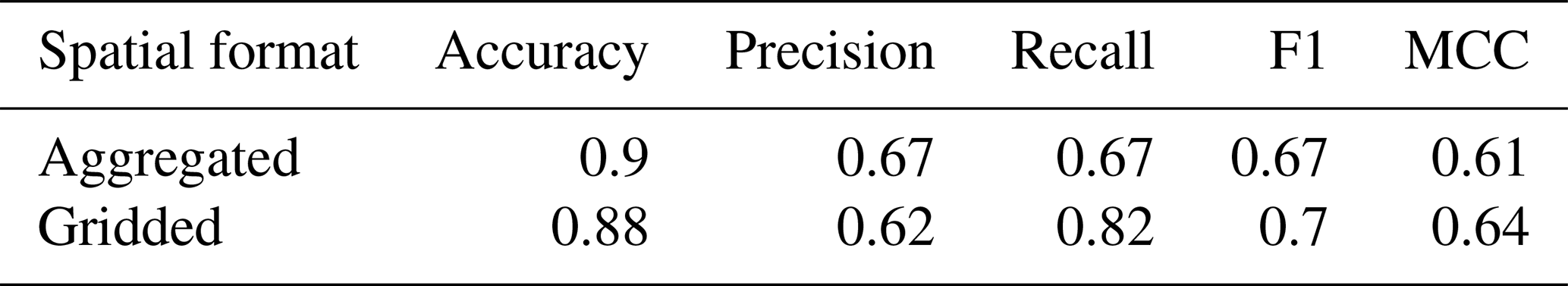
Table C2 Rank of the most important features for different feature selection methods along the entire soybean growing season: ANOVA, mutual information selection, random forest classifier and χ². Variables considered are maximum monthly temperature (tmx), precipitation (precip), diurnal temperature range (dtr), vapour pressure (vap), potential evapotranspiration (pet) and cloud cover (cld). Numbers 7 and 8 indicate the months of July and August, respectively.

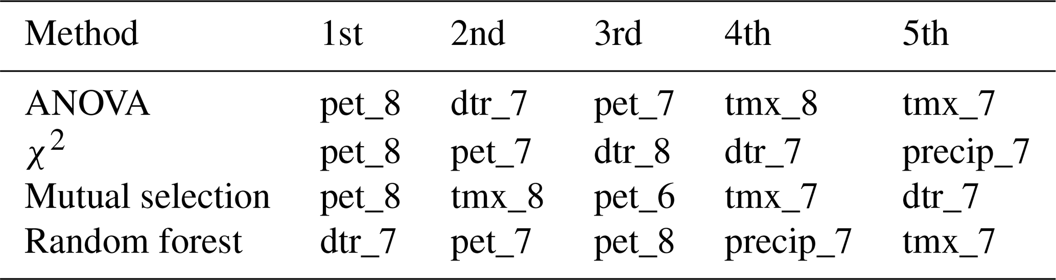
Table C3 Comparison of the random forest model performance between monthly data and aggregated data along reproductive phase of soybean growing season.

Table C4 Random forest model configuration of hyperparameters.