the Creative Commons Attribution 4.0 License.
the Creative Commons Attribution 4.0 License.
 | 26 Nov 2021
Reduced-complexity model for the impact of anthropogenic CO2 emissions on future glacial cycles
Andrey Ganopolski
We propose a reduced-complexity process-based model for the long-term evolution of the global ice volume, atmospheric CO2 concentration, and global mean temperature. The model's only external forcings are the orbital forcing and anthropogenic CO2 cumulative emissions. The model consists of a system of three coupled non-linear differential equations representing physical mechanisms relevant for the evolution of the climate–ice sheet–carbon cycle system on timescales longer than thousands of years. Model parameters are calibrated using paleoclimate reconstructions and the results of two Earth system models of intermediate complexity. For a range of parameters values, the model is successful in reproducing the glacial–interglacial cycles of the last 800 kyr, with the best correlation between modelled and global paleo-ice volume of 0.86. Using different model realisations, we produce an assessment of possible trajectories for the next 1 million years under natural and several fossil-fuel CO2 release scenarios. In the natural scenario, the model assigns high probability of occurrence of long interglacials in the periods between the present and 120 kyr after present and between 400 and 500 kyr after present. The next glacial inception is most likely to occur ∼50 kyr after present with full glacial conditions developing ∼90 kyr after present. The model shows that even already achieved cumulative CO2 anthropogenic emissions (500 Pg C) are capable of affecting the climate evolution for up to half a million years, indicating that the beginning of the next glaciation is highly unlikely in the next 120 kyr. High cumulative anthropogenic CO2 emissions (3000 Pg C or higher), which could potentially be achieved in the next 2 to 3 centuries if humanity does not curb the usage of fossil fuels, will most likely provoke Northern Hemisphere landmass ice-free conditions throughout the next half a million years, postponing the natural occurrence of the next glacial inception to 600 kyr after present or later.
- Article
(7323 KB) - Full-text XML
- BibTeX
- EndNote


The long-term evolution of the Earth system is not only of theoretical interest but a matter of utter practical relevance at present when its assessment is required in the decision-making process for guaranteeing the safe permanent storage of radioactive waste. The safe disposal of such materials constitutes one of the urgent environmental and societal challenges that mankind faces in the 21st century. Disposal in deep geologically stable rock formations is the only currently viable option to ensure long-term safety (International Atomic Energy Agency, 2007; Kim et al., 2011). While low- and intermediate-level nuclear waste requires at least 100 kyr years of safe storage, for high-level nuclear waste and spent nuclear fuel safety for 1 Myr should be envisaged. The evaluation of geological disposal systems in response to future environmental changes, driven by a combination of natural and anthropogenic forcings, is therefore mandatory.
Numerous paleoclimate records show that during the last 2.7 Myr the natural evolution of the Earth system has been characterised by persistent alternations of glacial and interglacial episodes. The last 800 kyr were dominated by strongly asymmetric glacial cycles with average periodicity of about 100 kyr, a rather slow glacial build-up, and much more rapid deglaciations (Hays et al., 1976; Lisiecki and Raymo, 2005). Antarctic ice core records show that the atmospheric carbon dioxide (CO2) concentration fluctuated nearly synchronously with the global ice volume and that the CO2 concentration during glacial times was up to 100 ppm lower than during preindustrial times (Petit et al., 1999; Lüthi et al., 2008). The astronomical theory of glacial cycles (Milankovitch, 1941) postulates that growth and shrinkage of ice sheets are primarily controlled by changes in Earth's orbital parameters (eccentricity, obliquity, and precession) through their effect on the amount of solar radiation received at high latitudes of the Northern Hemisphere (NH) during boreal summer. Different aspects of Milankovitch theory have been tested and supported with climate and Earth system models of different degrees of complexity (e.g. Pollard, 1983; Berger et al., 1999; Ganopolski and Calov, 2011; Abe-Ouchi et al., 2013; Tabor and Poulsen, 2016; Willeit et al., 2019).
For the future million years, however, not only natural processes are of relevance. It has been shown that anthropogenic CO2 emissions can affect future climate variability at very long timescales (Archer et al., 1997; Lenton and Britton, 2006; Ridgwell and Hargreaves, 2007). Even already achieved cumulative anthropogenic emissions of the order of 500 Pg C, when assuming no negative carbon emission in the future, can postpone the onset of the next glaciation by at least 50 kyr, while an emission of 5000 Pg C could completely change climate variability over the next 0.5 Myr (Archer and Ganopolski, 2005; Ganopolski et al., 2016).
The modelling of the climate evolution at 1 Myr timescales is not “accessible” for complex Earth system models and remains problematic even for most of the intermediate-complexity models due to prohibitive computational cost. Moreover, while Earth orbital parameters are accurately known for the next millions of years (Laskar et al., 2004), large uncertainties associated with the total amount of future fossil-fuel combustion require a computationally efficient modelling approach which permits the performance of numerous long-term simulations to assess impact of these uncertainties.
Most simple (conceptual) models of glacial cycles (e.g. Imbrie and Imbrie, 1980; Paillard, 1998; Tziperman et al., 2006; Crucifix, 2012) simulate only the response of global ice volume to orbital forcing and are thus not suitable for an assessment of long-term consequences of anthropogenic CO2 emission. Some simple models also describe CO2 concentration (for example, Saltzman, 1987; Saltzman and Verbitsky, 1993), but these models are designed only for description of the natural evolution of the carbon cycle. Thus, to our knowledge, there is no computationally inexpensive modelling tool which can simulate the future evolution of the global ice volume and CO2 concentration in response to anthropogenic perturbation.
To provide a set of possible scenarios of the future coupled climate–ice sheet–carbon cycle evolution we develop a reduced-complexity model based on paleoclimate data and results of physically based Earth system models. This approach constitutes a significant further development of the method proposed in Archer and Ganopolski (2005) and Lord et al. (2019). In the former, Paillard's conceptual model of glacial cycles was combined with the results of future CO2 simulations performed with a simple marine carbon cycle. In the latter, Palliard's model was combined with simulations of the future evolution of the anthropogenic CO2 anomaly modelled as in Lord et al. (2016) based on results of the Earth system model of intermediate complexity cGENIE (Lenton et al., 2007).
In this paper, a more advanced semi-empirical model is calibrated using paleoclimate records from the last 800 kyr and the results of the CLIMBER-2 Earth system model of intermediate complexity (EMIC) (Petoukhov et al., 2000; Ganopolski et al., 2001), while the future evolution of the anthropogenic CO2 anomaly is modelled following Lord et al. (2019, 2016).
We organise the paper as follows. In Sect. 2 we introduce the model and datasets. In Sect. 3 we present the model calibration. In Sect. 4 we present the results of the simulations for the next 1 Myr, considering scenarios with and without anthropogenic influence. In Sect. 5 we analyse the sensitivity of the results to several aspects of the model design and parameter selection strategy. Finally, in Sect. 6 we summarise the results and present the conclusions.
2.1 Modelling approach
We develop a process-based model for the coupled evolution of global ice volume (v), atmospheric CO2 concentration (CO2), and global mean surface air temperature (T). For the past, the model's only external forcing is orbital forcing. For the future, we additionally account for the impact of cumulative anthropogenic CO2 emissions on the atmospheric CO2 concentration. The model consists of a system of three coupled non-linear differential equations describing Earth system evolution at timescales from thousands to millions of years. While the model is designed for simulations of future glacial cycles, global temperature is a useful diagnostic which can become necessary in other potential applications.
It has been shown (Crucifix, 2012) that very different conceptual models of glacial cycles, based on completely different assumptions, can simulate past glacial cycles with similar and sufficiently high skill. Thus, paleodata alone are not sufficient to select the “right” model. Our approach to the construction of such a model is principally different from previous studies because the model is designed based on the results of physically based Earth system climate models. In particular, based on the CLIMBER-2 model simulations, (1) we define orbital forcing as the maximum summer insolation at 65∘ N; (2) for any orbital forcing at least one stable equilibrium is required and for a certain range of orbital forcings two equilibria (Calov and Ganopolski, 2005); (3) the transition from an interglacial to glacial state occurs when the insolation drops below a certain threshold value, which linearly depends on the logarithm of CO2 concentration (Ganopolski et al., 2016). We only selected model realisations which have this relationship consistent with the analysis presented in Ganopolski et al. (2016) (see discussion below).
For model calibration, we use a hybrid approach based on a combination of paleodata and CLIMBER-2 model simulations. We use paleoclimate reconstructions of the late Quaternary (last 800 kyr; see below). This period was selected for two reasons: (1) so far this is the only period of time for which accurate reconstructions of the atmospheric CO2 concentration are available, and (2) this period is dominated by long glacial cycles which are expected to continue in the future, at least for some time in the absence of significant anthropogenic influence (see discussion below). However, during that period the CO2 atmospheric concentration was lower than preindustrial levels most of time and always below the present one. Therefore, those records alone are insufficient to derive a model suitable for modelling future climate evolution under anthropogenic influence. Given the lack of accurate CO2 reconstructions from periods with a CO2 atmospheric concentration higher than the preindustrial level, we calibrate the model behaviour in such a greenhouse world using results of the physically based CLIMBER-2 model. The selected model realisations are used to simulate the next million years under natural and several anthropogenic scenarios. Future CO2 concentration scenarios were computed using results of the studies performed with the cGENIE EMIC. Since there are no available simulations of CO2 concentration under the combined effect of anthropogenic CO2 emissions and future ice sheet growth (growth that can only happen after the CO2 anomalies decrease considerably) we assume that natural and anthropogenic CO2 anomalies can be simply added up.
2.2 Equation for global ice volume
The first model equation describes the temporal evolution of global ice volume v expressed in non-dimensional units (with a value of 1 corresponding to the reconstructed Last Glacial Maximum – LGM, 21 kyr before present – ice volume). Since it is set that at present v=0, this variable in fact represents the anomaly of global ice volume relative to the preindustrial state. As the principal natural forcing for global ice volume is summer NH insolation this equation is only valid for NH ice volume. To account for the contribution of the Southern Hemisphere (SH), we use the same approach as in Ganopolski and Calov (2011) and assume that the ice volume anomaly in the SH closely follows the NH anomaly and makes up a constant, relatively small faction of the global ice volume anomaly. This approach, obviously, is not applicable for possible future Antarctic and Greenland ice sheet melting under high CO2 concentrations. This is why we do not consider future sea level rise above the preindustrial level, and it is required that v≥0 at any time (see below).
Although the constraint of v≥0 for the future is a strong one, we expect the approach not to be a problem even under the most pessimistic anthropogenic scenario we consider in this paper (cumulative emissions of 3000 Pg C). On one hand, a scenario leading to the complete melting of the Greenland ice sheet would change the global ice volume by a small value compared to the glacial–interglacial variability and could thus be neglected. On the other hand, a complete Antarctic deglaciation would definitely affect the global climate carbon cycle and could not be ignored. However, according to Garbe et al. (2020), significant Antarctic mass loss occurs only if the global temperature anomaly stays above 8 ∘C for a very long time, and, as a consequence, even under the 3000 Pg C emission scenario the contribution of the Antarctic ice sheet to changes in global ice volume could be neglected, at least to a first approximation (see below for the estimated temperature change under different anthropogenic scenarios).
The mass-conservation equation states that
“Accumulation” here represents the global ice accumulation (in mass per time units) and “ablation” represents all mass losses from ice sheets including surface and basal melt, as well as iceberg calving. We assume that the total accumulation is proportional to the total ice sheet area (Ganopolski et al., 2010). In turn, ice sheet area is closely related to the ice volume. It is often assumed that A=vγ, where γ is about 0.8. Here for simplicity we assume γ=1, and thus
where b is the proportionality constant.
On the other hand, ablation is controlled by several processes of which the energy balance at the surface of the ice sheets is the most important one. Total ablation depends on the size of the ice sheets (and in the NH, especially on the position of their southern margin), summer insolation (orbital forcing), and CO2 atmospheric concentration (CH4 and N2O also play a role but we assume their radiative forcing to be proportional to the radiative forcing of CO2 as in Willeit et al., 2019). The effect of CO2 on the mass balance of an ice sheet is introduced via the logarithm of its concentration because radiative forcing of CO2 is proportional to the logarithm of concentration. As the metric for orbital forcing we use the maximum summer insolation at 65∘ N computed using Laskar et al. (2004). To reproduce a rapid deglaciation process we introduce an additional term proportional to . To ensure existence of at least one equilibrium solution (solution with ) for any combination of orbital and CO2 forcing (Calov and Ganopolski, 2005; Abe-Ouchi et al., 2013) a negative term proportional to the ice volume in power large than 1 is required. Here to this end we use the term since it gives a better model performance. Thus, the total ablation is represented as
where b01 to b5 are constants, is the average orbital forcing, and Mv is a memory term that reflects the history of the ice volume during the last τ years as long as is negative. At any time t, Mv(t) is defined as
Finally, the mass balance (Eq. 1) is rewritten as
where and b6 are additional model parameters.
2.3 Equation for atmospheric CO2 concentration
It is generally recognised that CO2 (together with other well-mixed greenhouse gases such as CH4 and N2O) represents an important amplifier of glacial cycles and that the anthropogenic CO2 emissions will affect the climate during long periods of time (Archer and Brovkin, 2008), in particular the timing and magnitude of future glacial cycles (Archer and Ganopolski, 2005). Although the mechanisms of glacial–interglacial atmospheric CO2 variability are still not fully understood, significant progress in modelling the global carbon cycle operation during glacial cycles has been achieved in recent times (Brovkin et al., 2012; Menviel et al., 2012; Willeit et al., 2019). Since CO2 and ice volume are highly correlated (during the past 800 kyr the coefficient of correlation between atmospheric CO2 concentration and ice volume is −0.71), it is not surprising that simple conceptual models of glacial cycles can describe the ice volume evolution without an explicit treatment of CO2 (e.g. Paillard, 1998; Crucifix, 2013). However, this close relationship between CO2 and global ice volume is not valid for the Anthropocene, and thus modelling the future climate evolution requires an explicit treatment of the atmospheric CO2 concentration, which is the second equation of our model. The response of the global carbon cycle to external perturbations involves a broad range of timescales: from very short (annual) to geological. For the purpose of this study we treat natural and anthropogenic anomalies of CO2 separately but consider them additive. Namely, we assume that on the relevant timescales (103–105 years), the natural component of the CO2 concentration is in equilibrium with external conditions and is expressed through a linear combination of global temperature and global ice volume.
The most direct effect of temperature on CO2 is through changes in the CO2 solubility in ocean water (Zeebe and Wolf-Gladrow, 2001). Temperature, directly and through sea ice, also affects ocean circulation (Watson et al., 2015), ventilation rate of the deep water (Kobayashi et al., 2015), changes in relative volume of different water masses (Brovkin et al., 2007), and metabolic rates of living organisms (Eppley, 1972; Laws et al., 2000).
The direct effect of ice volume on CO2 changes is less straightforward (note that the strong effect of ice sheets on atmospheric temperature is already accounted for in the temperature term). An increase in ice volume leads to a decrease in the ocean volume and, as a consequence, increased ocean salinity. As CO2 solubility in the ocean decreases with salinity this would provoke an increase in the atmospheric CO2 concentration, counteracting the temperature effect (Zeebe and Wolf-Gladrow, 2001). Higher global ice volume would also mean a smaller area of the globe is covered by forests and therefore diminished carbon storage in the terrestrial reservoir, driving an increase in atmospheric CO2 (Prentice et al., 2011). Increased glacial supply of iron-rich dust may help suppress the iron limitation in some areas (in particular in the South Atlantic Ocean), leading to increased biological productivity and thus lower atmospheric CO2 levels (Martin, 1990; Watson et al., 2000).
In addition, based on results of Ganopolski and Brovkin (2017) we parameterised CO2 “overshoots” during glacial terminations by an additional term proportional to . Note that this additional term is only applied when . The justification for such parameterisation is the results seen in many models (Gottschalk et al., 2019) that a shutdown of the Atlantic Meridional Overturning Circulation (AMOC) causes an atmospheric CO2 rise of about 10–20 ppm. A shutdown of the AMOC is caused by a large meltwater flux, which is in turn controlled by changes in ice volume (i.e. ).
To describe the anthropogenic component of CO2, we assume that anthropogenic CO2 emission is a relatively short (of the order of 102 years) pulse followed by zero emissions. In this case, the temporal dynamics of the anthropogenic component of the CO2 anomaly depend only on the cumulative carbon emissions. To describe the long anthropogenic tail of CO2 (Anth term in the Eq. (7) below) we use the analytical parameterisation defined in Lord et al. (2016) based on the results of experiments with the Earth system model of intermediate complexity cGENIE (Lenton et al., 2007). In addition, we assume that natural and anthropogenic CO2 anomalies can be simply summed up and that in preindustrial times the global carbon cycle was in equilibrium. This is, obviously, a very strong assumption since even a rather small imbalance in the global carbon cycle, which is impossible to detect at millennial timescales, can result in a very large “drift” of the Earth system from its preindustrial state at the million-year timescale. However, due to the absence of any practical alternative, we proceeded with this assumption.
After these considerations, the equation that governs the CO2 evolution has the following shape:
where c1 to c4 are adjustable model parameters. The first three terms on the right-hand side of Eq. (7) represent the already discussed effects of global temperature (T), ice volume, and AMOC weakening or shutdown. The fourth term (c4) is simply a constant, and the last term represents the effect of anthropogenic CO2 emissions. Refer to Sect. 4.1 for a detailed explanation on the assumptions and shape of the function Anth.
2.4 Equation for global mean surface temperature
The last equation in our model describes the global mean surface air temperature anomaly (relative to preindustrial values) as a linear combination of two terms: first, the direct effect of global ice volume (the larger the ice volume, the higher the planetary albedo and the lower the global temperature) and, second, a term representing the radiative forcing of CO2, which is proportional to the logarithm of CO2 concentration:
where d1 and d2 are adjustable model parameters.
2.5 Model constraints
The model of past and future glacial cycles is represented by the system of three equations (Eqs. 6, 7, 8) which contains three variables (v, CO2, and T), orbital forcing f(t), anthropogenic CO2 anomaly Anth, and 12 parameters (bi i=1–6; cj j=1–4, dk k=1–2). The orbital forcing f(t) is determined by astronomical parameters (eccentricity, precession, and obliquity), which are accurately known for the entire period of interest (Laskar et al., 2004). The function Anth is assumed to be null until t=0 kyr; afterwards the function depends only on time and cumulative CO2 emissions as detailed in Sect. 4.1.
Model parameters are calibrated to yield solutions that are in good agreement with both the paleoclimatic information over the last 800 kyr (see Sect. 2.6 for details on the paleoclimate reconstructions used) and CLIMBER-2 results.
We impose on the model a series of constraints based on paleorecords from the last 800 kyr: (1) reproduction of present-day interglacial state, (2) reproduction of LGM conditions, (3) mid-Brunhes transition (MBT), and (4) compliance with CO2 minimum level.
For the first constraint, based on the observational fact that the present state is an interglacial one, we require that
This condition fixes the value for c4 at 278.
As the confidence in empirical data for glacial conditions is higher at LGM than at any other glacial episode, the accurate reproduction of LGM conditions is important. At LGM, the empirical ice volume in non-dimensional units was 1, CO2 concentration 194 ppm, and global cooling around 5 ∘C (Schneider et al., 2006; Annan and Hargreaves, 2013; Tierney et al., 2020). We then require from the model that
It is known that glacial cycles prior to the MBT about 400 kyr ago differ in some respects from those after the MBT. In particular, pre-MBT interglacials were characterised by lower CO2 and higher benthic δ18O values than the post-MBT episodes. The latter implies a large interglacial, probably due to remaining continental ice sheets in the NH. The mechanisms accounting for these differences are still not understood (Tzedakis et al., 2009), but they are unlikely related to differences in orbital forcing before and after MBT. This is why it is not expected that a simple model forced by orbital variations alone can simulate such behaviour. Thus, we prescribe that before the MBT the minimum ice volume must be 0.05 in normalised units.
The last condition based on empirical data prevents CO2 from dropping to levels significantly lower than the minimum atmospheric CO2 concentration registered in the last 800 kyr by paleorecords (172 ppm) at any given moment in time.
We also impose a condition related to the current estimates for the equilibrium climatic sensitivity (ECS), i.e. global temperature response to a doubling in atmospheric CO2 concentration from preindustrial levels. We select equilibrium climate sensitivity (ECS) equal to 3.9 ∘C, which coincides with the multi-model mean in the Coupled Model Intercomparison Project 6 (CMIP6; Zelinka et al., 2020):
Equations (10) and (14) determine the values for the coefficients d1 and d2 at −3 and 5.56, respectively.
Recent studies (e.g. Nijsse et al., 2020) suggest that some CMIP6 models have unrealistically high ECS, and the IPCC AR6 report proposed a best estimate for ECS of 3 ∘C. However, on the long timescales considered in this paper, the classical ECS, which accounts only for fast climate feedback but not for the feedbacks related to vegetation, ice sheets, and atmospheric composition (apart from CO2), likely underestimates the Earth system response to radiative perturbation. Nonetheless, to assess uncertainties in future climate simulations associated with uncertainties in ECS, we performed an additional set of simulations with ECS = 3 ∘C (see Sect. 5).
In addition, we account for several modelling studies (Berger and Loutre, 2002; Cochelin et al., 2006; Ganopolski et al., 2016) indicating that the conditions for the new glacial inception will not be met in the near future even in the absence of anthropogenic influence on climate. To ensure that our model satisfies this requirement, we require for all valid model versions the average global ice volume not to exceed 0.025 (in normalised units) in the time period between 0 and 20 kyr:
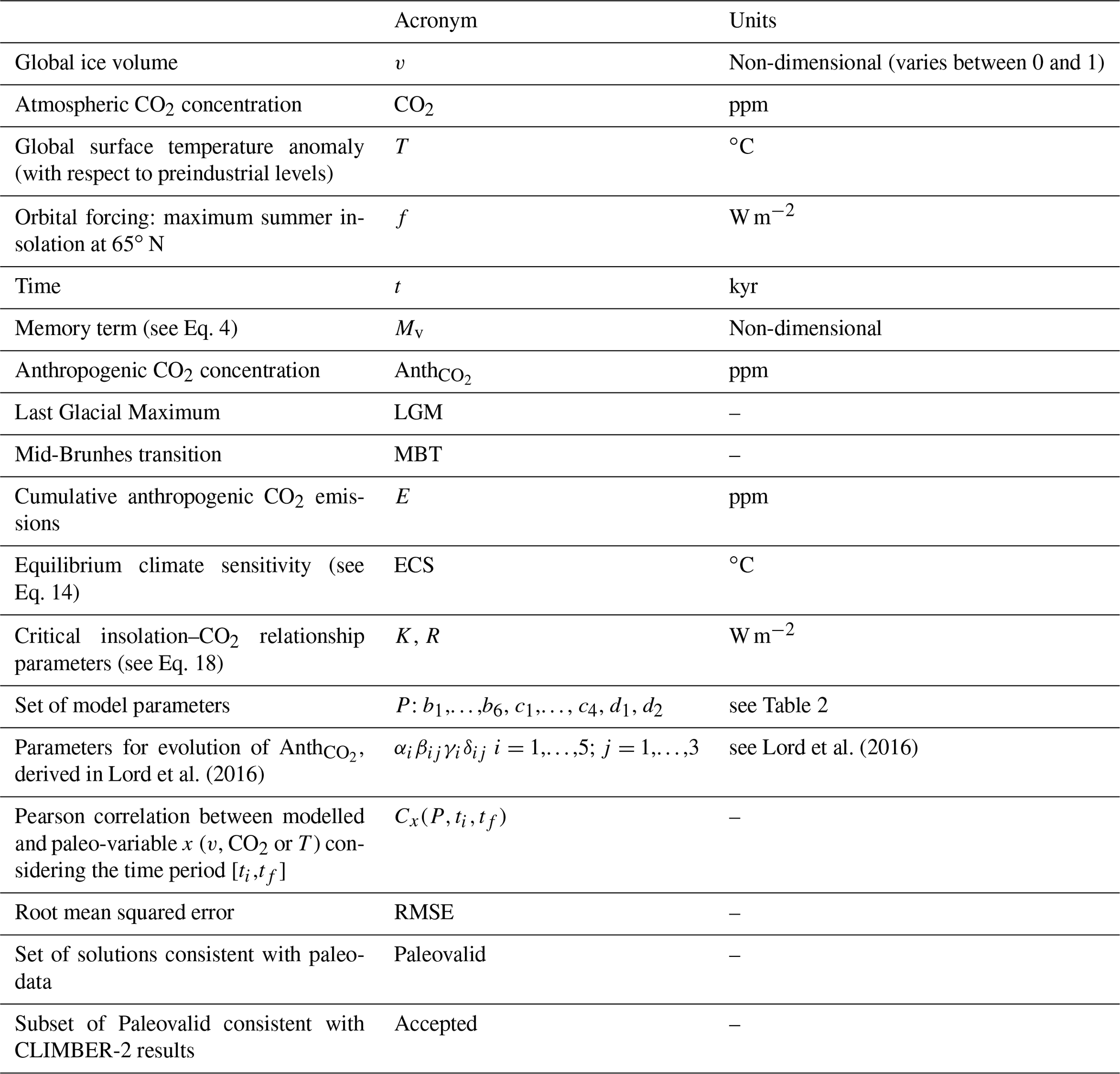
For the Base experimental setting (other settings will be discussed in Sect. 5), the model is defined by Eqs. (6)–(8) together with the conditions expressed in Eqs. (9)–(15). A table of acronyms (Table 1) is provided as a quick reference.
In this section we describe the choice of model parameters using paleoclimate data and CLIMBER-2 modelling results. First, we select a range of model parameters which enable us to simulate the past evolution of global ice volume, CO2, and global temperature with reasonable accuracy (see Sect. 3.2). We call this set of model realisations Paleovalid. We then apply an additional constraint based on the critical insolation–CO2 relationship for glacial inceptions, which is of fundamental importance for the prediction of future glacial cycles in the response to anthropogenic CO2 emissions. Since we find that paleodata do not provide additional constraints on this relationship (see Sect. 3.3), we consider the estimation of the critical insolation–CO2 curve derived from CLIMBER-2 in Ganopolski et al. (2016) and take forward only those solutions in line with it. All model realisations which satisfy this criterion are named Accepted, and we use them for future scenarios simulations.
3.1 Empirical datasets
Paleo-reconstructions covering the period [−800, 0 kyr] are used as part of the learning and/or validation sets for the model. Reconstructed global ice volume is derived from sea level stack (Spratt and Lisiecki, 2016). Past CO2 atmospheric concentration levels are derived from ice cores records (Lüthi et al., 2008). For global mean surface temperature anomalies (with respect to preindustrial conditions) we use two reconstructions: (1) Friedrich et al. (2016), which covers the period [−784, −10 kyr], and (2) Snyder (2016), covering [−800, −1 kyr]. All datasets are transformed into time series with a 1 kyr time step.
Obviously, the paleoclimate reconstructions are not perfect and have associated uncertainties. While information for global ice volume and CO2 atmospheric concentration is based directly on paleoclimate records and considered quite accurate, global temperature reconstructions are based on a limited number of local temperature records, mostly from ocean sites, and have large uncertainties (as easily noticeable in the two paleorecords in Fig. 1c).
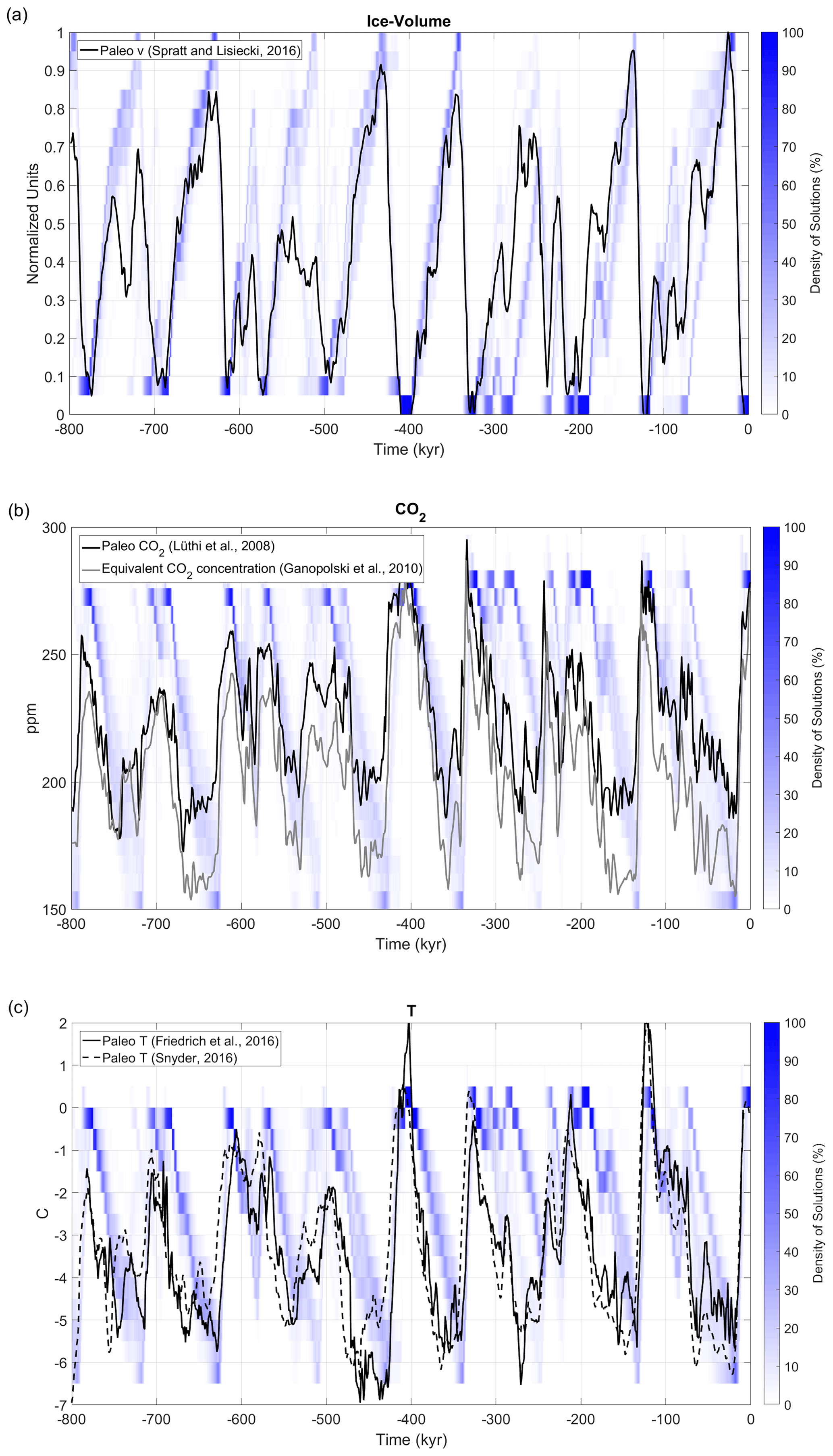
Figure 1Paleovalid solutions and paleoclimatic records in the period [−800, 0 kyr]: (a) global landmass ice volume (normalised to unity); reconstruction (black line) from Spratt and Lisiecki (2016). (b) Atmospheric CO2 concentration (ppm), paleorecord (black line) from Lüthi et al. (2008), and equivalent CO2 concentration from Ganopolski et al. (2010) (grey line). (c) Global mean surface temperature anomaly (C); paleorecords from Friedrich et al. (2016) (solid black) and Snyder (2016) (dashed). Blue shaded areas represent the density of Paleovalid solutions per unit of phase space (units are 1 kyr for time, 0.05 for ice, 7 ppm for CO2, and 0.5 ∘C for temperature).
3.2 Calibration using paleoclimate reconstructions
For each set of parameters P, we calculate v, CO2, and T using the system of Eqs. (6)–(8) and denote them as vmodel(P), CO2model(P), and dTmodel(P).
We approach the task of the selection of a set of parameters P as a non-linear optimisation problem with constraints. We wish to find P to maximise the optimisation target function Cv:
where vmodel(P) (ti,tf) denotes the modelled ice volume time series in the period [ti,tf], vPaleo(ti,tf) denotes the paleo-ice volume time series in the period [ti,tf], and corr(x,y) denotes the linear Pearson correlation between x and y. The time interval for the optimisation is set to . See Appendix A for a discussion of the dependence of model performance on the choice of this time interval. To select parameters that will optimise correlation at the same time as providing magnitudes in accordance with empirical estimations, an equality constraint is enforced: the maximum ice volume must be equal to 1 within a tolerance of 0.15 (in non-dimensional units). Equation (14) is enforced as an inequality constraint.
The time step for the calculation of the time series is 1 kyr. We use the interior-point optimisation algorithm under the MATLAB environment. Approximately 1000 optimisation routines were performed, each starting from a different combination of the set of nine adjustable parameters (optimisation seeds).
Finally, the ensemble of valid solutions, Paleovalid, is defined as
The correlation level of 0.7, although arbitrary, guarantees a good fit to the paleoclimatic ice volume record. For the selection of solutions, no conditions are imposed on the goodness of fit between modelled and paleo-CO2 or temperature.
Naturally, there are many possible choices for model calibration procedures. In particular, it is possible to select a different optimisation target function. We chose to optimise the correlation between modelled and paleo-ice volume because our main objective is to simulate future glacials, and thus the reproduction of these cycles is extremely relevant. Livadiotis and McComas (2013) present the maximisation of the correlation fitting method. Those authors show that the method is mathematically well defined under certain conditions and that it should be preferred over the classical least squares fitting in situations in which the datasets exhibit variations that need to be described, such as is the case for glacial cycles. The sensitivity of our results to a different optimisation target is evaluated in Sect. 5. While we opt for a frequentist perspective (estimates of unknown parameters are obtained without assigning them probabilities) parameter estimation can also be approached through a Bayesian point of view (e.g. Crucifix and Rougier, 2009).
Figure 1 displays the ensemble probabilistic distribution of solutions in Paleovalid for v, CO2, and T as well as the corresponding paleoclimatic data for the period [−800, 0 kyr]. The ranges of the different model parameters across the Paleovalid set are displayed in Table 2.
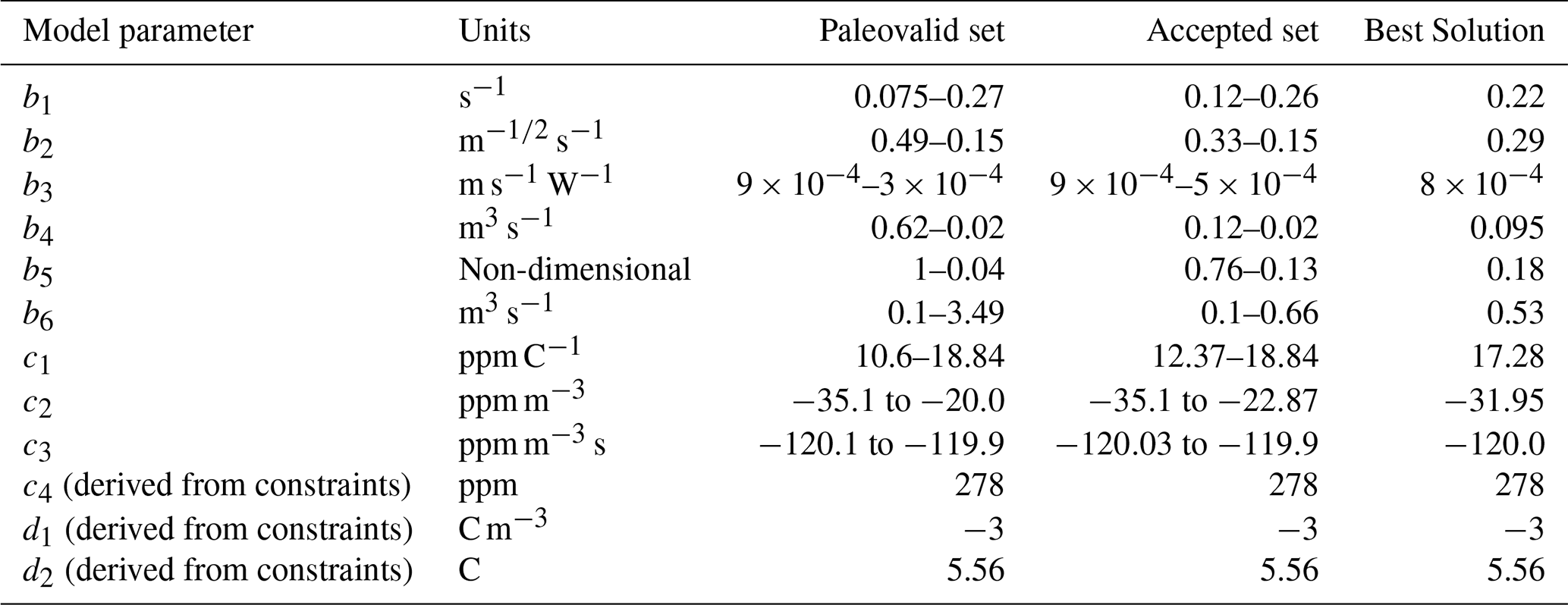
Table 2Parameter ranges across solutions in the Paleovalid and Accepted sets as well as for the Best Solution.
By definition, all the solutions derived from the Paleovalid ensemble closely follow the paleo-ice volume curve (Fig. 1a), with the ensemble mean correlation between modelled and paleo-ice volume in [−800, 0 kyr] equal to 0.76. While most of the solutions derived from Paleovalid succeed in capturing the timing and magnitude of the major glaciations, there is a tendency for them to overestimate the ice volume in MIS 18 and MIS 14 (−560 and −520 kyr, respectively). As model parameters were chosen to maximise ice volume correlation only, it is expected that the performance in terms of CO2 and global temperature will be inferior to that for global ice volume. The ensemble mean correlation between modelled and paleo-CO2 is 0.5, and approximately 50 % of the solutions display an amplitude range significantly larger than the observed one, reaching the imposed lower limit of 150 ppm (Fig. 1b). Note, however, the better magnitude agreement when comparing simulated CO2 with the equivalent CO2 concentration (as computed in Ganopolski et al., 2010) and which accounts for the additional radiative effect of N2O and CH4. The imperfect CO2 simulations, however, represent no major pitfall for a skilful ice volume reproduction, as shown by the 0.76 ensemble mean correlation with paleodata. Interestingly, when using accurately known CO2 time series from ice cores, this ensemble mean correlation for global ice volume is only slightly increased to 0.85. For global mean surface temperature (Fig. 1c), the ensemble mean correlation between modelled and paleorecords is 0.56, and the solutions' amplitude ranges within the paleo-estimation limits.
While the model demonstrates a good performance when tested against the same data used for its training, its ability to produce predictions (situation in which previously unseen data are used as model input) can only be evaluated by the use of independent training and validation samples. A robust estimation of the model's predictive skill, using disjoint training and validation sets, is found in Appendix A. In general, we conclude that the model also has a satisfactory ability when used in predictive mode, and thus we confidently venture to utilise it as a tool for the assessment of possible future scenarios.
3.3 Glacial inception: critical insolation–CO2 relationship
Using an ensemble of CLIMBER-2 model realisations consistent with paleoclimatic constraints, Ganopolski et al. (2016) found that the critical threshold for summer insolation at 65∘ N to trigger glacial inception is described by the following curve:
where W m−2 and R=466 W m−2.
The parameter K is a measure of the sensitivity of the critical orbital forcing to the atmospheric CO2 concentration. The higher K is, the more important CO2 is; i.e. for the same CO2 emission scenario, the effect of anthropogenic perturbation on glacial cycles will last longer.

Figure 2Histogram for K (see Eq. 17) across the different members of the Paleovalid ensemble of solutions. Red bars correspond to the Accepted solutions.
Following the Ganopolski et al. (2016) approach, we calculate the corresponding coefficient K for each of the ensemble members in the Paleovalid set (Fig. 2). For the estimation of K we refer to Eq. (6); assuming equilibrium and interglacial conditions (i.e. , v=0, Mv=0) the critical insolation threshold is derived as
It follows then that K is estimated as .
Table 3Summary of Paleovalid and Accepted ensemble characteristics.

Our results indicate that with the model derived in this study the possible values of the coefficient K range between −1279 and −31 W m−2, with a median of −393 W m−2. This highlights the fact that, even though all the solutions derived from the Paleovalid set have a high level of agreement with the paleoclimatic records along last 800 kyr, the relationship between fcritial and log(CO2) is not constrained by paleoclimate data; i.e. model realisations with completely different values of K can produce similarly good agreement with the paleoclimate reconstructions. However, for the future simulations different K values lead to very different impacts of anthropogenic CO2 emissions on the Earth system evolution. This is why for performing future simulations we select only Paleovalid solutions which are consistent with CLIMBER-2 simulations. However, since Ganopolski et al. (2016) present only single values for the K parameter and did not perform any uncertainty analysis of K, we applied a rather “soft” constraint on its value; namely, it should satisfy the condition W m−2. Even such soft constraints lead to a dramatic reduction of the remaining model realisations, which we call “Accepted” and which consists of only 29 members. A summary of the characteristics of the Paleovalid and Accepted ensembles is found in Table 3. The probabilistic distribution of solutions for v, CO2, and T derived from Accepted is displayed in Fig. 4, and the ranges of the different model parameters across Accepted are found in Table 2.
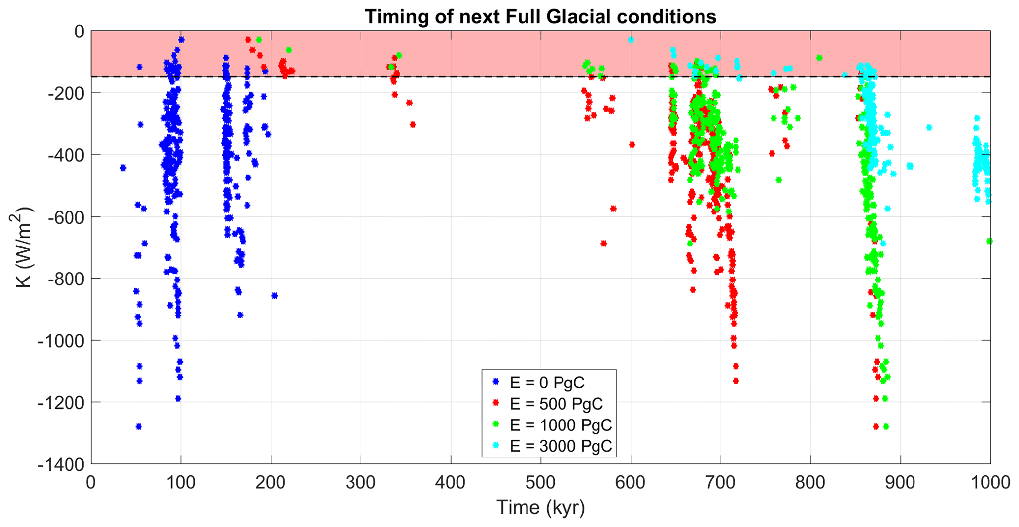
Figure 3Dependence of the timing of the next full glacial conditions (v=0.5) on the parameter K for all solutions in Paleovalid and under the different emission scenarios considered. The red shaded area indicates the solutions in the Accepted set.
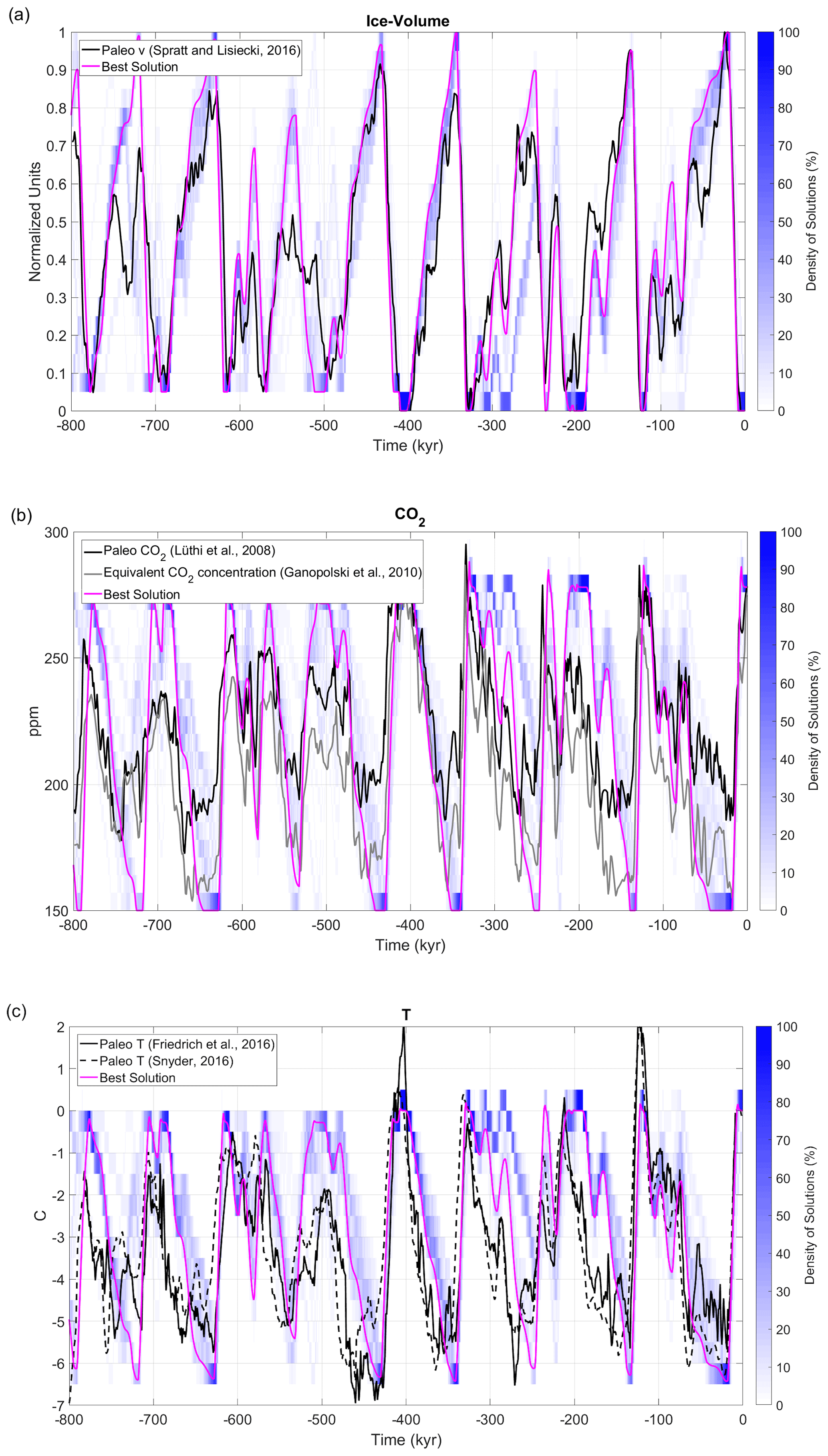
Figure 4Same as Fig. 1 but for solutions in the Accepted ensemble. In addition, magenta lines show the evolution of the Best Solution.
In the next section we present results of future simulations and use only Accepted model versions. However, to demonstrate the importance of additional constraints on the value of K, we also perform future simulations with all Paleovalid versions. Figure 3 illustrates these results through the timing of the first (after the present) full glacial conditions as a function of K. Not surprisingly, for the natural scenario, there is no clear dependence on K and the first full glacial conditions are predicted 100 or 200 kyr from the present. The situation is very different for the scenarios with anthropogenic emissions. For example, for low (500 Pg C) emissions, the model versions with a K value satisfying the criteria for the Accepted model version predict the next full glacial conditions around 200 kyr from the present. However, most of the model versions with higher K predict the next full glacial conditions 700 kyr and even 900 kyr from the present. The situation is similar for other anthropogenic scenarios. This analysis clearly shows the importance of applying a tight constraint on the K value to produce realistic future scenarios.
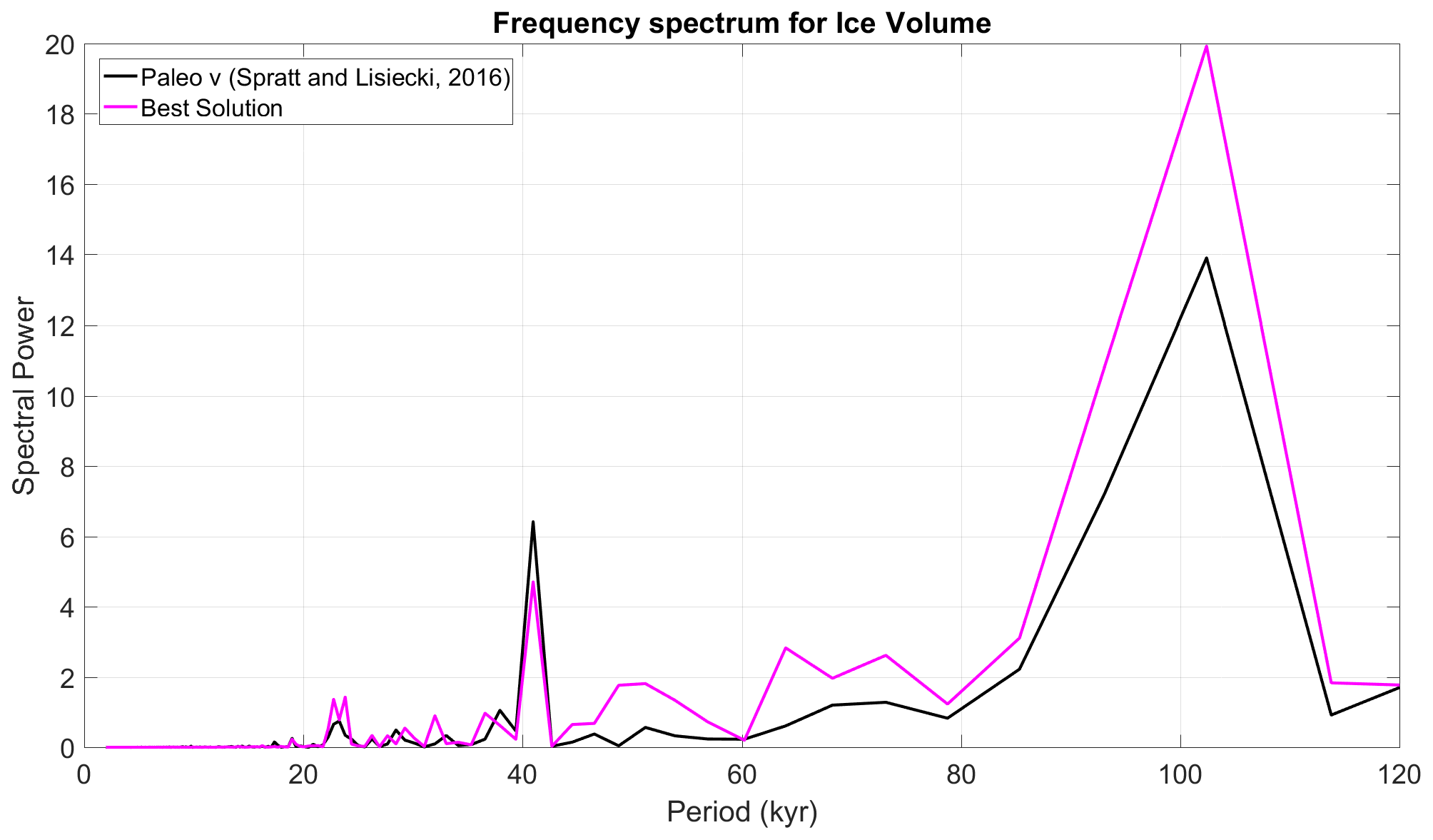
Figure 5Frequency spectrum for simulated (Best Solution, magenta) and reconstructed ice volume (Spratt and Lisiecki, 2016; black).
In addition, we define the Best Solution PBest as
PBest values are shown in Table 2. The time series for , , and are shown in Fig. 4. The model version named Best Solution is rather successful in reproducing the observed climatic variability in the three considered variables for the whole [−800, 0 kyr] period. The model skill in reproducing both the temporal variability and amplitudes of the time series fluctuations is remarkable. In particular, the performance for ice volume is excellent, with a correlation between the model and paleodata of 0.86 (Fig. 4a). The model is able to correctly capture the timing of all the glaciations, with the LGM being the highest-volume event. The ice volume model and paleorecord discrepancy is largest for MIS 18 ([−750, −710 kyr]). The frequency spectra of and the empirical estimation are also in good agreement (Fig. 5): there is a clear dominant peak at 100 kyr, with additional power at 41 and 23 kyr. For the atmospheric CO2 concentration, the correlation between modelled and recorded series is 0.62 (Fig. 4b). While the model succeeds in reproducing glacial–interglacial variability, it overestimates its magnitude at around 130 ppm instead of 80 ppm. It is, in particular, evident that during interglacials the CO2 restores to its equilibrium value of 278 ppm, which according to the paleorecords is not accurate before the MBT. Finally, the correlation between modelled and global paleo-mean surface temperature anomalies is 0.54 (Fig. 4c). The model slightly underestimates the variability of this variable, ranging between 0 and −5 ∘C, while the observational information suggests a larger range between 2 and −7 ∘C. The high positive temperature anomalies during some previous interglacials, however, are questionable.
In this section we present results of simulations of the evolution of the Earth system in the next 1 Myr under natural and several anthropogenic emissions scenarios using the Accepted model ensemble.
4.1 CO2 emission scenarios
Future scenarios are generated considering different temporal evolution paths for the excess atmospheric CO2 concentration, which we assume depends only on the cumulative amount of fossil-fuel combustion, Anth (see Eq. 7). For the natural scenario, Anth is set to zero at all times, and, as a consequence, the climate system follows its natural evolution forced only by changes in orbital forcing.
For the fossil-fuel emission scenarios, we consider instantaneous releases of CO2 at t=0 of different magnitudes. If the duration of the emission pulse release is rather short (centuries) and is followed by zero CO2 emissions, the future long-term evolution of CO2 depends primarily on the cumulative emission magnitude, while the rate of release is only of secondary relevance (Eby et al., 2009). For the period 1750–2017, estimations place the fossil-fuel cumulative emissions in carbon equivalent at 660±95 Pg C (Le Quéré et al., 2018). Projections for future cumulative emissions range between ∼700 and ∼3000 Pg C, with the former being an estimate of fossil-fuel reserves exploitable with today's technical and economic constraints and the latter an estimation considering reserves that might become exploitable in the future (McGlade and Ekins, 2015). Taking into account the already achieved and future cumulative emissions estimations, we generate three different scenarios: low, intermediate, and high emissions, corresponding to instantaneous pulse releases of magnitude 500, 1000, or 3000 Pg C, respectively. In each scenario, after the pulse release, Anth follows a multi-exponential decay function as proposed by Lord et al. (2016).
Here, E (Pg C) represents the cumulative fossil-fuel emission magnitude, the constant 0.469 transforms units (Pg C to ppm) of CO2, and Anth is expressed in units of parts per million (ppm).
Parameter values (αiβijγiδij i=1,…, 5; j=1,…, 3) are derived in Lord et al. (2016) in order to produce a good fit to a series of 1 Myr pulse-type experiments performed with the cGENIE EMIC (Lenton et al., 2007). Lord et al. (2016) consider total anthropogenic CO2 emissions ranging between 0 and 20.000 Pg C; the latter value is justified assuming future techno-economic advances could make additional non-conventional resources such as methane clathrates available for extraction. The use of results from long-term simulations with the cGENIE model represents a substantial improvement compared to Archer and Ganopolski (2005), who used CO2 scenarios obtained with a simple marine carbon cycle model which did not explicitly account for a climate–weathering feedback.
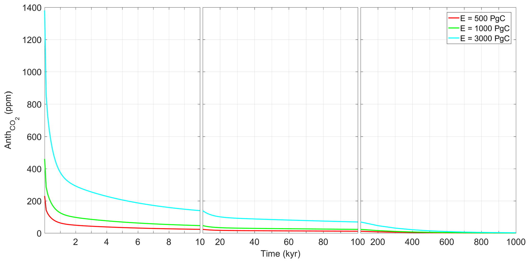
Figure 6Anth expressed in parts per million (ppm) following Lord et al. (2016) for the three different emission scenarios considered.
The function Anth from the present until 1 million years into the future under the low-, intermediate-, and high-emissions scenarios is shown in Fig. 6. Approximately 100 kyr after the (low, intermediate, or high) emissions pulse release ∼5 % of the initial CO2 anomaly is still present in the atmosphere. For the low-emissions scenario, only 500 kyr after the pulse emission do the remaining anthropogenic CO2 concentration anomalies drop below 1 % of the original perturbation, marking the return of the system to its natural state. For the medium- and high-emission scenarios, the return to natural conditions takes even longer.

Figure 7Simulated ice volume for different future scenarios: (a) natural scenario, (b) low-emissions scenario (E=500 Pg C), (c) intermediate-emissions scenario (E=1000 Pg C), and (d) high-emissions scenario (E=3000 Pg C). The magenta line depicts the behaviour of the Best Solution, and the blue shades represent the density of Accepted solutions per unit of phase space (units are 1 kyr for time and 0.05 for ice).
4.2 Possible future natural Earth system trajectories
Figure 7a displays future global ice volume evolution for the Best Solution and the probabilities of the trajectories of individual model realisations. It shows both periods of high agreement and periods of high discrepancy between solutions, highlighting the co-existence of more certain (deterministic) and less certain aspects of the Earth system response to orbital forcing. Most of the solutions agree that the planet will remain in a long interglacial state for the next 50 kyr, during which no large ice growth is expected (however, there is one solution in which glacial inception starts at 20 kyr and full glacial conditions are reached by 36 kyr). This behaviour is predefined by one of the model constraints, namely that v should be equal to zero at present and by a weak orbital forcing during the next 20 kyr. With a high level of confidence, a second long interglacial is expected to occur between 450 and 500 kyr, which is another prolonged period of weak orbital forcing related to the 400 kyr periodicity of eccentricity. Also with high certainty, short (∼10 kyr) interglacials are expected to occur 110, 230, 250, 270, 370, 620, 820, and 900 kyr from the present.
In the conceptual model we define full glacial conditions to occur when the ice volume (v) reaches 0.5 in normalised units. If full glacial conditions are reached at a time T, then the corresponding glacial inception is defined as the first time before T in which v>0:
Following those definitions, regarding the timing of the next full glacial conditions the solutions tend to cluster into two different possibilities: predicted to occur in ∼90 kyr or in ∼150 kyr (see also Fig. 3). For those cases, the glacial inception occurs at ∼50 or ∼110 kyr, respectively. There is also some level of certainty in the timing of occurrence of major glaciations (defined here as periods with ice volume higher than 0.8 in normalised units): ∼100, ∼210, ∼410, ∼450, ∼680, ∼790, ∼870, and 950 kyr from the present. The possible future scenario indicates that only two of these major glaciations (the ones ∼210 and ∼870 kyr after the present) have a high probability of reaching LGM magnitudes (∼1 in normalised units).

Figure 8Ice volume time series for each solution in Accepted for the intermediate-emissions scenario (E=1000 Pg C). Each solution is coloured according to its corresponding K value.
If we consider the possible future scenario produced by the trajectory of the Best Solution (Fig. 8) as the most likely path, under natural circumstances (1) the next glacial inception is expected to occur ∼50 kyr after present (with full glacial conditions reached ∼90 kyr after present); (2) in the next 1 Myr two long interglacials should take place, and (3) nine major glaciations are expected, all of them with maximum magnitudes around 10 %–15 % lower than LGM level. The natural glacial cycles of the future are strongly dominated by 100 kyr cyclicity as were the past ones.
4.3 Possible future trajectories under different anthropogenic CO2 emissions scenarios
The evolution of the ice volume even in the low-emissions anthropogenic scenario (E=500 Pg C, which is lower than already emitted) is significantly different from the natural one in the next 200 kyr, indicating a long-lasting impact of fossil-fuel CO2 releases (Fig. 7b). The uncertainty levels for the next 150 kyr and from 400 to 500 kyr are greatly reduced, with most of the solutions agreeing on ice-free NH conditions. Under this scenario, only after half a million years is the Earth system able to return to an evolution similar to the one expected under natural conditions. Under this setting, the next full glacial conditions are not expected to be able to occur before 180 kyr from the present, implying a delay of at least 90 kyr from the natural expected evolution, which is consistent with Archer and Ganopolski (2005) and Ganopolski et al. (2016). In particular, the ice volume evolution of the Best Solution under this scenario differs significantly from the natural one during two periods: [0, 200 kyr] and [400, 500 kyr]. In both time spans glaciations fail to be triggered for this scenario (Figs. 7b and 8a). In [200, 350 kyr] the low-emissions Best Solution trajectory is similar to the natural one, except for a lag of ∼10 kyr. CO2 and global mean surface temperature anomaly (Fig. 8b and c) pathways are also restored to natural conditions only after 500 kyr from the present.
For the intermediate case (E=1000 Pg C) the effect of anthropogenic CO2 emissions on the Earth system is even more long-lasting. The ensemble of possible future scenario indicates significantly different conditions from the natural ones in the next half a million years, with a very low probability of considerable ice growth during the totality of this time span (Fig. 7c). In most of the solutions full glacial conditions occur for the first time either in ∼550 kyr or between 600 and 700 kyr from the present (Fig. 3). In particular, the Best Solution is part of the latter group, with the next full glacial condition taking place only ∼670 kyr after the present. Additional insight into the relevance of the parameter K for future behaviour under anthropogenic influence is presented in Fig. 8: the larger the magnitude of K, the larger the delay in the next glacial inception.
Finally, with a cumulative emission of 3000 Pg C, the Earth system is expected, with high confidence, to experience almost ice-free conditions for the next 600 kyr (Fig. 7d). Under this scenario, the next full glacial conditions are not expected to occur before 670 kyr from the present, implying a lag of almost 600 kyr from the natural scenario. For example, in the Best Solution, only two major glaciations are predicted, peaking in 880 kyr with a magnitude 20 % lower than LGM (Figs. 7d and 9a). In the 3000 Pg C scenario, half a million years into the future, CO2 is expected to be 300 ppm (22 ppm higher than preindustrial levels) and the global mean surface temperature still 0.5 ∘C higher than the preindustrial level (Fig. 9b and c).

Figure 9Best Solution under different emission scenarios: (a) ice volume (normalised to unity), (b) CO2 (ppm), (c) global mean surface temperature anomalies (C).
Table 4Summary of settings for sensitivity experiments.
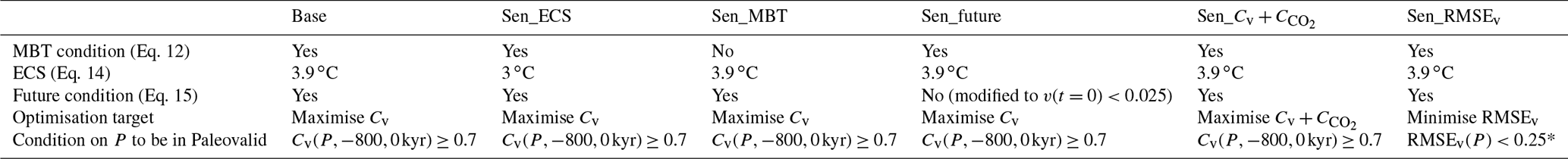
* 0.25 corresponds to the RMSE of forecasting the average ice volume in the period [−800, 0 kyr].
In order to assess the robustness of the results to the model or parameter selection strategy, we performed a series of sensitivity experiments. Table 4 summarises the settings for the Base experimental setup and five different sensitivity experiments. For each experiment, the optimisation process is carried out, and Paleovalid and Accepted sets of solutions are created (the definition of the Paleovalid might change from the standard one in Eq. 17 in some of the experiments; see Table 4). As a summary of results, Fig. 10 depicts the range of timings of the next full glacial conditions for each experiment and anthropogenic emissions scenario.
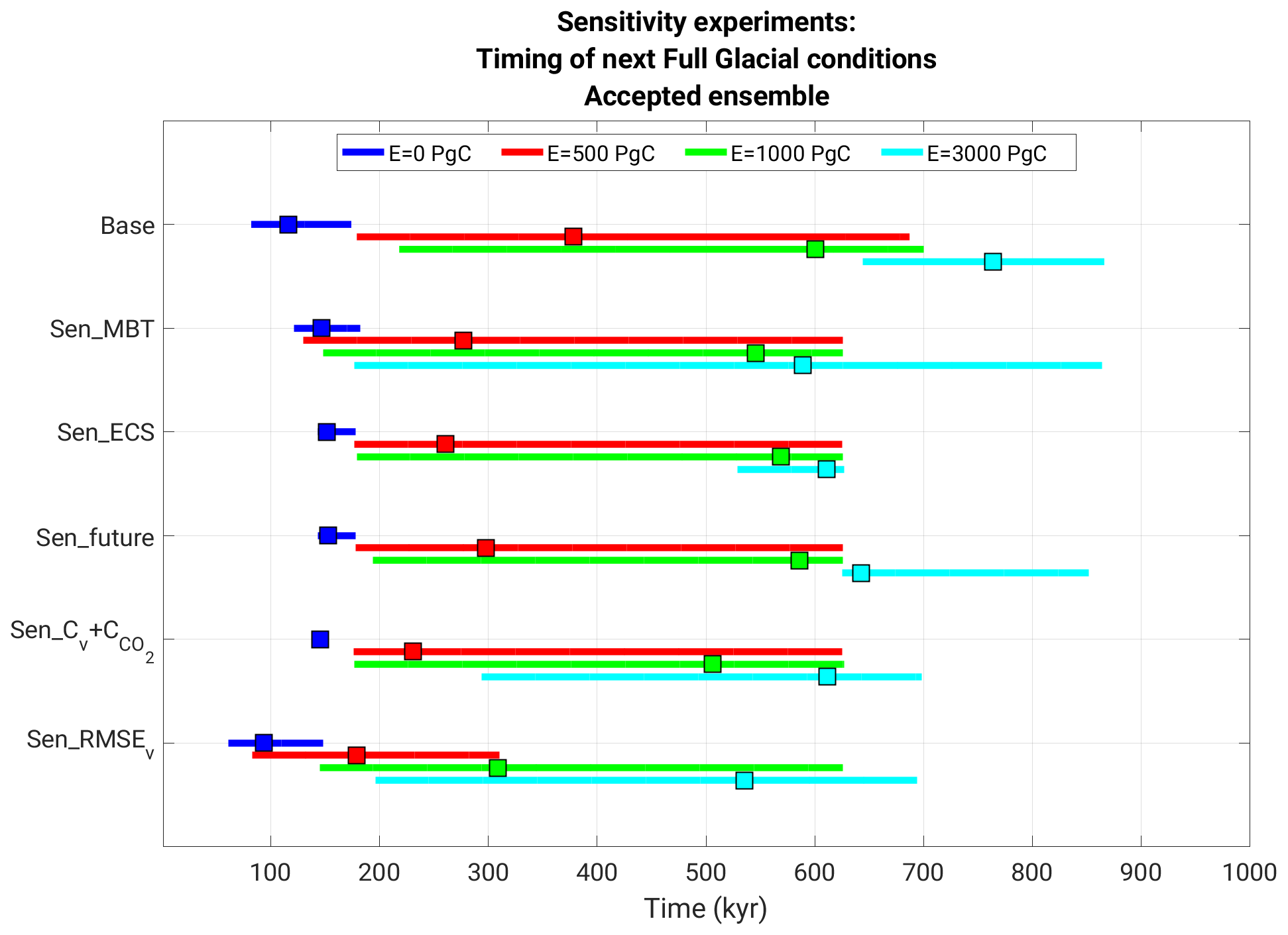
Figure 10Timing of next full glacial conditions (first time after present when v=0.5) for different model configurations and emission scenarios, considering the Accepted solutions. For a certain configuration and emission scenario, line segments indicate the 5 %–95 % percentiles of the timings, while squares indicate the ensemble mean.
In the first sensitivity experiment (Sen_MBT) the ad hoc imposition related to MBT (Eq. 12) is lifted. Naturally, the correlation between modelled and paleo-ice volume in Sen_MBT is slightly lower than in the base model formulation (the ensemble mean across Accepted drops from 0.79 to 0.72). The ensemble mean timing of the next full glacial conditions under the natural, low-, and intermediate-emissions scenarios for this setting does not substantially differ for the one in the Base experimental configuration. For the high-emissions scenario, though, the timing for next full glacial conditions spans the full 200–860 kyr period, with the ensemble mean being around 600 kyr in the future (∼150 kyr earlier than in Base).
Second, we test the sensitivity of the results to the choice of ECS of the model. We report on the results ensuring an ECS of 3 ∘C (instead of 3.9 ∘C in Eq. 14). The results of this experiment (Sen_ECS) indicate that the main conclusions are not overly sensitive to the change in the selected ECS for the natural, low-, and intermediate-emissions scenarios. However, for the high-emissions scenario the timing of the next full glacial conditions is confined to 520–620 kyr, which is somewhat earlier than expected using the Base configuration.
In the third experiment, Sen_future, we modify Eq. (15) so that it does not include any conditions on the future. Without this constraint, the new Paleovalid ensemble contains three solutions (out of 400 ensemble members) for which glacial inception occurs at some point between the present and 20 kyr into the future. However, those solutions do not fulfil the requirements for being included in Accepted. The main results remain largely unchanged with respect to the Base experiment.
Fourth and fifth, we test the sensitivity of the results to the selected optimisation metric. In the fourth experiment (Sen_Cv_) we select parameters in order to jointly maximise correlations between modelled and paleo-ice volume and CO2. For that purpose we maximise .
We find that for the Sen_Cv_ (Base) experiment the Accepted ensemble mean correlation between modelled and paleo-ice volume is 0.71 (0.79) and between modelled and paleo-CO2 is 0.55 (0.5), therefore showing similar performance in terms of correlations. The most notorious difference between this and the Base setting occurs in the natural scenario, for which the majority of the solutions agree that the next full glacial conditions will develop 130 kyr from the present.
In the fifth experiment, instead of optimising correlations, we select parameters to minimise the root mean squared error (RMSE) between modelled and paleo-ice volume. Using an RMSE instead of a correlation optimisation strategy leads to the strongest changes in the timing of the next full glacial conditions for the low- and intermediate-emissions scenarios: the ensemble mean occurs ∼200 and ∼300 kyr earlier than in the Base configuration, respectively. While these differences in the ensemble mean behaviour are substantial, the spread of possible timings within the Accepted set is still comparable.
We propose a reduced-complexity process-based model of the evolution of global ice volume, atmospheric CO2 concentration, and global mean temperature at multi-millennial and orbital timescales. The model's only external forcings are the orbital forcing and (for the future) anthropogenic CO2 cumulative emissions. The model consists of a system of three coupled non-linear differential equations representing physical mechanisms relevant for the evolution of the climate–ice sheet–carbon cycle system. Model parameters are selected to achieve the best possible agreement with reconstructed ice volume variations during the past 800 kyr and consistency with CLIMBER-2 model results. Global temperature anomaly at the Last Glacial Maximum and the current best estimate for the equilibrium climate sensitivity have been used as additional constraints on model parameters. Furthermore, the solutions are bounded to account for the difference between pre- and post- mid-Brunhes transition interglacial conditions, and a minimum for the CO2 concentration is set to avoid unrealistic solutions.
The model is successful in reproducing the natural glacial–interglacial cycles of the last 800 kyr, in agreement with paleorecords, replicating both the timing and amplitude of the major fluctuations, with a correlation between modelled and reconstructed global ice volume of up to 0.86. The model also shows a promising performance when evaluated against data not used for training, indicating a certain skill in predictive mode.
Using different model realisations we generate an ensemble of possible future trajectories for the evolution of the Earth system over the next 1 million years under natural and three different anthropogenic CO2 emission scenarios.
In the natural scenario, in which anthropogenic CO2 emissions are assumed to be zero at all times, the model assigns high probability of occurrence of (1) long interglacials in two periods: from 0 to ca. 50 kyr after the present and between 400 kyr and 500 kyr after the present. The next glacial inception will most likely occur ∼50 kyr after the present with the development of full glacial conditions ∼90 kyr after present. It is also clear, however, that even though there is a high level of agreement in the trajectories during the past 800 kyr, their paths tend to diverge for the future, indicating that the past does not perfectly constrain the future evolution of the climate–ice sheet–carbon cycle system.
The selected model versions exhibit a large sensitivity to fossil-fuel CO2 releases, with even already achieved emissions (500 Pg C) causing a behaviour significantly different from the natural one over extremely long periods of time. The model predicts that a fossil-fuel CO2 release of 500 Pg C will make the beginning of the next Ice Age highly unlikely in the next 120 kyr, and a delay of half a million years is a possibility that cannot be ruled out. Cumulative fossil-fuel CO2 emissions of the order of 3000 Pg C (which could be achieved in the next 2 to 3 centuries if humanity does not cease fossil-fuel usage; Meinshausen et al., 2011) will most likely lead to ice-free conditions over the NH continents throughout the next half a million years. Under this scenario, the probability for the next glacial inception to occur before 600 kyr is extremely low. Thus, our study demonstrates that, in spite of large uncertainties in model parameters, there is a qualitative difference in the long-term Earth system trajectories (Steffen et al., 2018) between cumulative emissions of 500 and 3000 Pg C.
However, it is clear that large uncertainties pose serious challenges to our ability to model the deep future. First, the present study reveals that the results are very sensitive to the relationship between the critical insolation threshold for glacial inception and CO2 levels. In turn, this relationship is poorly constrained by the paleoclimatic data because during previous interglacials CO2 was similar to or lower than the preindustrial CO2 level. So far, this relationship has been analysed only with the CLIMBER-2 model (Calov and Ganopolski, 2005; Ganopolski et al., 2016). This is why in this work, we assumed the uncertainty in this relationship to be 100 %. Performing experiments similar to those described in Ganopolski et al. (2016) but with more advanced Earth system models can help to reduce uncertainties in future projections. Second, knowledge of the long-term (105–106 years) carbon cycle dynamics remains poor, primarily because of the lack of accurate empirical data. In particular, the results from Lord et al. (2016) used in this paper to simulate the decay of excess CO2 in the atmosphere are largely theoretical and based on the assumption that the long-term carbon cycle is regulated solely through silicate weathering, omitting the role of other possible processes (i.e. organic carbon burial in marine sediments, kerogen weathering).
We consider our approach potentially useful in providing projections of the possible future Earth system evolution. However, it has a number of limitations. In particular, one key assumption of our procedure is that ice volume is equal to or higher than the preindustrial level at all times. While a possible future melting of Greenland will not substantially affect this hypothesis, a possible future melting of Antarctica definitely will. Therefore, we must emphasise that the methodology presented here is not applicable for anthropogenic scenarios in which a substantial melting of the Antarctic ice sheet could be expected (cumulative emissions higher than 3000 Pg C).
When a model is developed with a predictive goal (like in this study), it is important to have an assessment of its predictive skill. The best possible estimations of this skill are obtained by evaluating how well the model performs when presented with previously unseen data.
To follow the cross-validation assessment criterion (Stone, 1974), we divide the period [−800, 0 kyr] into halves: P1 = [−800, −400 kyr] and P2 = [−400, 0 kyr]. First, P1 is labelled the training set and P2 the validation set. Second, the model is trained using the information in P1: we run the optimisation scheme to maximise the correlation between modelled and paleo-ice volume during P1; we then accept all the models (parameter combinations) yielding correlations higher than 0.7. Third, all the accepted models are validated using the information in P2. We select three different performance metrics: the correlation between modelled and paleo-ice volume, between modelled and paleo-CO2, and between modelled and global mean surface temperature anomaly calculated during P2. Finally, we repeat the previous three steps but labelling P1 as the validation set and P2 as the training set. For each metric, the average that the models achieve on the two possible validation sets considered is the estimate of the model's predictive skill.
Table A1Estimation of model predictive skill. Only solutions leading to a correlation between modelled and paleo-estimation of ice volume higher than 0.7, calculated over the training period, are considered. See text for more details on the training and validation periods used.
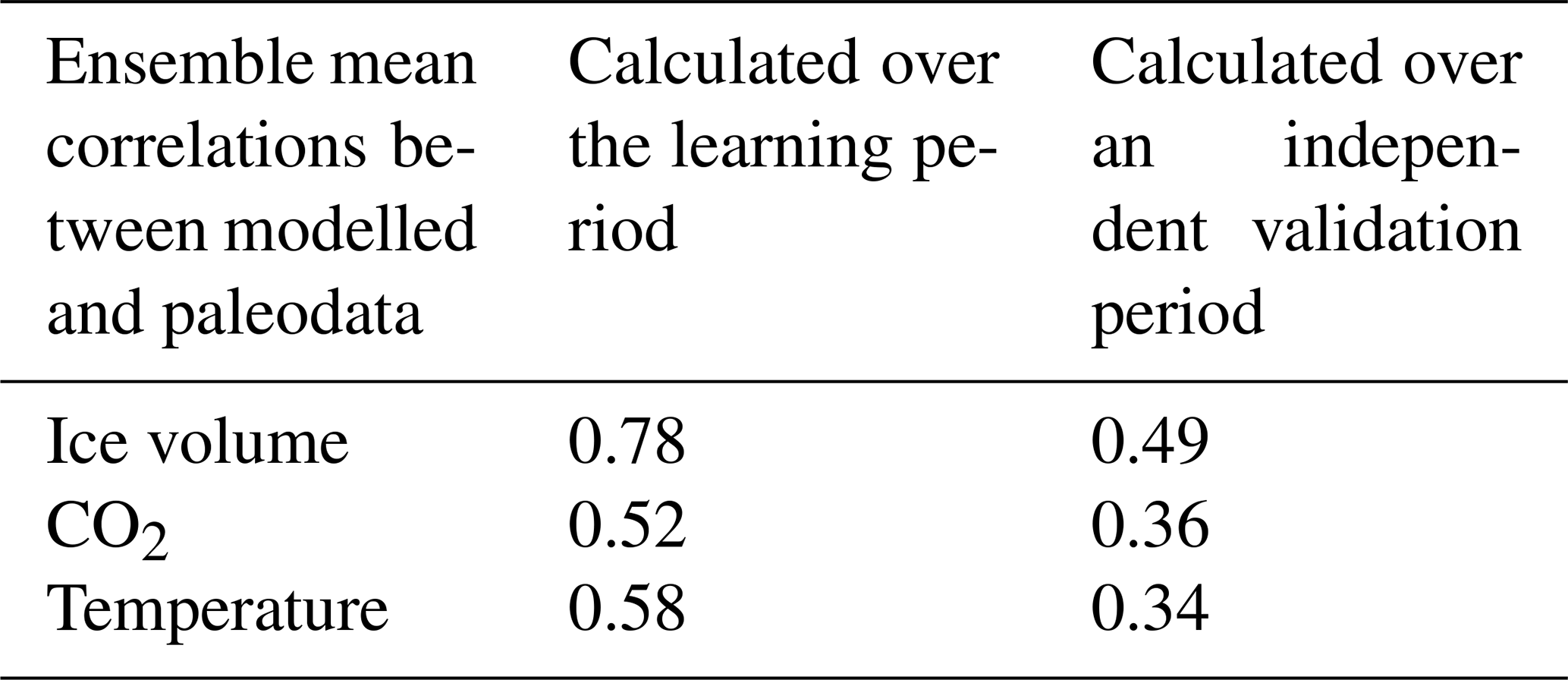
In Table A1 we summarise the results of this cross-validation assessment, showing the results for the three performance metrics. For reference, Table A1 also displays the values of the metrics when calculated over the training period (instead of over the validation period). Results are the average of two possible cases: P1 as the training set and P2 as the validation set or P2 as the training set and P1 as the validation set. As expected, when the same period is used for both model training and evaluation, the results are in better agreement with paleoclimate data: the ice volume metric is 0.78, the CO2 metric 0.52, and the temperature metric 0.58. These values drop to 0.49, 0.36, and 0.34 respectively, when the independent validation set is used to calculate the metrics. Even though the drop in performance is not negligible, the model skill is still substantial, in particular for predicting ice volume.
Code and data used in this study can be obtained from https://doi.org/10.17605/OSF.IO/KB76G (Talento, 2021).
AG conceived the original idea. ST performed all the calculations and produced figures. Both authors contributed to the analysis of results and writing of the paper.
The authors declare that they have no conflict of interest.
Publisher's note: Copernicus Publications remains neutral with regard to jurisdictional claims in published maps and institutional affiliations.
We thank three anonymous referees, Mikhail Verbitsky, Alan Kennedy-Asser, and Jens Becker, for valuable comments that helped improve the quality of the paper.
Financial support for this study was provided by the Swiss National Cooperative for the Disposal of Radioactive Waste (NAGRA).
This paper was edited by Gabriele Messori and reviewed by three anonymous referees.
Abe-Ouchi, A., Saito, F., Kawamura, K., Raymo, M. E., Okuno, J., Takahashi, K., and Blatter, H.: Insolation-driven 100,000-year glacial cycles and hysteresis of ice-sheet volume, Nature, 500, 190–193, https://doi.org/10.1038/nature12374, 2013.
Annan, J. D. and Hargreaves, J. C.: A new global reconstruction of temperature changes at the Last Glacial Maximum, Clim. Past, 9, 367–376, https://doi.org/10.5194/cp-9-367-2013, 2013.
Archer, D. and Brovkin, V.: The millennial atmospheric lifetime of anthropogenic CO2, Clim. Change, 90, 283–297, https://doi.org/10.1007/s10584-008-9413-1, 2008.
Archer, D. and Ganopolski, A.: A movable trigger: Fossil fuel CO2 and the onset of the next glaciation: Next Glaciation, Geochem. Geophys. Geosyst., 6, Q05003, https://doi.org/10.1029/2004GC000891, 2005.
Archer, D., Kheshgi, H., and Maier-Reimer, E.: Multiple timescales for neutralization of fossil fuel CO2, Geophys. Res. Lett., 24, 405–408, https://doi.org/10.1029/97GL00168, 1997.
Berger, A. and Loutre, M. F.: An exceptionally long interglacial ahead?, Science, 297, 1287–1288, 2002.
Berger, A., Li, X. S., and Loutre, M. F.: Modelling northern hemisphere ice volume over the last 3Ma, Quaternary Sci. Rev., 18, 1–11, https://doi.org/10.1016/S0277-3791(98)00033-X, 1999.
Brovkin, V., Ganopolski, A., Archer, D., and Rahmstorf, S.: Lowering of glacial atmospheric CO 2 in response to changes in oceanic circulation and marine biogeochemistry: Mechanisms of lowering glacial pCO2, Paleoceanography, 22, PA4202, https://doi.org/10.1029/2006PA001380, 2007.
Brovkin, V., Ganopolski, A., Archer, D., and Munhoven, G.: Glacial CO2 cycle as a succession of key physical and biogeochemical processes, Clim. Past, 8, 251–264, https://doi.org/10.5194/cp-8-251-2012, 2012.
Calov, R. and Ganopolski, A.: Multistability and hysteresis in the climate-cryosphere system under orbital forcing, Geophys. Res. Lett., 32, L21717, https://doi.org/10.1029/2005GL024518, 2005.
Cochelin, A.-S. B., Mysak, L. A., and Wang, Z.: Simulation of long-term future climate changes with the green McGill paleoclimate model: the next glacial inception, Clim. Change, 79, 381–401, https://doi.org/10.1007/s10584-006-9099-1, 2006.
Crucifix, M.: Oscillators and relaxation phenomena in Pleistocene climate theory, Phil. Trans. R. Soc. A., 370, 1140–1165, https://doi.org/10.1098/rsta.2011.0315, 2012.
Crucifix, M.: Why could ice ages be unpredictable?, Clim. Past, 9, 2253–2267, https://doi.org/10.5194/cp-9-2253-2013, 2013.
Crucifix, M. and Rougier, J.: On the use of simple dynamical systems for climate predictions, The European Physical Journal Special Topics, 174, 11–31, https://doi.org/10.1140/epjst/e2009-01087-5 ,2009.
Eby, M., Zickfeld, K., Montenegro, A., Archer, D., Meissner, K. J., and Weaver, A. J.: Lifetime of Anthropogenic Climate Change: Millennial Time Scales of Potential CO2 and Surface Temperature Perturbations, J. Climate, 22, 2501–2511, https://doi.org/10.1175/2008JCLI2554.1, 2009.
Eppley, R. W.: Temperature and phytoplankton growth in the sea, Fish. Bull., 70, 1063–1085, 1972.
Friedrich, T., Timmermann, A., Tigchelaar, M., Elison Timm, O., and Ganopolski, A.: Nonlinear climate sensitivity and its implications for future greenhouse warming, Sci. Adv., 2, e1501923, https://doi.org/10.1126/sciadv.1501923, 2016.
Ganopolski, A. and Brovkin, V.: Simulation of climate, ice sheets and CO2 evolution during the last four glacial cycles with an Earth system model of intermediate complexity, Clim. Past, 13, 1695–1716, https://doi.org/10.5194/cp-13-1695-2017, 2017.
Ganopolski, A. and Calov, R.: The role of orbital forcing, carbon dioxide and regolith in 100 kyr glacial cycles, Clim. Past, 7, 1415–1425, https://doi.org/10.5194/cp-7-1415-2011, 2011.
Ganopolski, A., Petoukhov, V., Rahmstorf, S., Brovkin, V., Claussen, M., Eliseev, A., and Kubatzki, C.: CLIMBER-2: a climate system model of intermediate complexity. Part II: Model sensitivity, Clim. Dynam., 17, 735–751, 2001.
Ganopolski, A., Calov, R., and Claussen, M.: Simulation of the last glacial cycle with a coupled climate ice-sheet model of intermediate complexity, Clim. Past, 6, 229–244, https://doi.org/10.5194/cp-6-229-2010, 2010.
Ganopolski, A., Winkelmann, R., and Schellnhuber, H. J.: Critical insolation–CO2 relation for diagnosing past and future glacial inception, Nature, 529, 200–203, https://doi.org/10.1038/nature16494, 2016.
Garbe, J., Albrecht, T., Levermann, A., Donges, J. F., and Winkelmann, R.: The hysteresis of the Antarctic ice sheet, Nature, 585, 538–544, https://doi.org/10.1038/s41586-020-2727-5, 2020.
Gottschalk, J., Battaglia, G., Fischer, H., Frölicher, T. L., Jaccard, S. L., Jeltsch-Thömmes, A., Joos, F., Köhler, P., Meissner, K. J., Menviel, L., Nehrbass-Ahles, C., Schmitt, J., Schmittner, A., Skinner, L. C., and Stocker, T. F.: Mechanisms of millennial-scale atmospheric CO2 change in numerical model simulations, Quaternary Sci. Rev., 220, 30–74, https://doi.org/10.1016/j.quascirev.2019.05.013, 2019.
Hays, J. D., Imbrie, J., and Shackleton, N. J.: Variations in the Earth's Orbit: Pacemaker of the Ice Ages, Science, 194, 1121–1132, https://doi.org/10.1126/science.194.4270.1121, 1976.
Imbrie, J., and Imbrie, J.: Modeling the climatic response to orbital variations, Science, 207, https://doi.org/10.1126/science.207.4434.943, 1980.
International Atomic Energy Agency, Spent Fuel and High Level Waste: Chemical Durability and Performance under Simulated Repository Conditions, TECDOC Series, Vienna (Austria), ISBN 978-92-0-106007-5, ISSN 1011-4289, 2007.
Kim, J.-S., Kwon, S.-K., Sanchez, M., and Cho, G.-C.: Geological storage of high level nuclear waste, KSCE J. Civ. Eng., 15, 721–737, https://doi.org/10.1007/s12205-011-0012-8, 2011.
Kobayashi, H., Abe-Ouchi, A., and Oka, A.: Role of Southern Ocean stratification in glacial atmospheric CO2 reduction evaluated by a three-dimensional ocean general circulation model: CO2 Response to Glacial Stratification, Paleoceanography, 30, 1202–1216, https://doi.org/10.1002/2015PA002786, 2015.
Laskar, J., Robutel, P., Joutel, F., Gastineau, M., Correia, A. C. M., and Levrard, B.: A long-term numerical solution for the insolation quantities of the Earth, A&A, 428, 261–285, https://doi.org/10.1051/0004-6361:20041335, 2004.
Laws, E. A., Falkowski, P. G., Smith, W. O., Ducklow, H., and McCarthy, J. J.: Temperature effects on export production in the open ocean, Global Biogeochem. Cycles, 14, 1231–1246, https://doi.org/10.1029/1999GB001229, 2000.
Lenton, T. M. and Britton, C.: Enhanced carbonate and silicate weathering accelerates recovery from fossil fuel CO 2 perturbations: Weathering accelerates removal of fossil fuel CO2, Global Biogeochem. Cycles, 20, GB3009, https://doi.org/10.1029/2005GB002678, 2006.
Lenton, T. M., Marsh, R., Price, A. R., Lunt, D. J., Aksenov, Y., Annan, J. D., Cooper-Chadwick, T., Cox, S. J., Edwards, N. R., Goswami, S., Hargreaves, J. C., Harris, P. P., Jiao, Z., Livina, V. N., Payne, A. J., Rutt, I. C., Shepherd, J. G., Valdes, P. J., Williams, G., Williamson, M. S., and Yool, A.: Effects of atmospheric dynamics and ocean resolution on bi-stability of the thermohaline circulation examined using the Grid ENabled Integrated Earth system modelling (GENIE) framework, Clim. Dynam., 29, 591–613, https://doi.org/10.1007/s00382-007-0254-9, 2007.
Le Quéré, C., Andrew, R. M., Friedlingstein, P., Sitch, S., Hauck, J., Pongratz, J., Pickers, P. A., Korsbakken, J. I., Peters, G. P., Canadell, J. G., Arneth, A., Arora, V. K., Barbero, L., Bastos, A., Bopp, L., Chevallier, F., Chini, L. P., Ciais, P., Doney, S. C., Gkritzalis, T., Goll, D. S., Harris, I., Haverd, V., Hoffman, F. M., Hoppema, M., Houghton, R. A., Hurtt, G., Ilyina, T., Jain, A. K., Johannessen, T., Jones, C. D., Kato, E., Keeling, R. F., Goldewijk, K. K., Landschützer, P., Lefèvre, N., Lienert, S., Liu, Z., Lombardozzi, D., Metzl, N., Munro, D. R., Nabel, J. E. M. S., Nakaoka, S., Neill, C., Olsen, A., Ono, T., Patra, P., Peregon, A., Peters, W., Peylin, P., Pfeil, B., Pierrot, D., Poulter, B., Rehder, G., Resplandy, L., Robertson, E., Rocher, M., Rödenbeck, C., Schuster, U., Schwinger, J., Séférian, R., Skjelvan, I., Steinhoff, T., Sutton, A., Tans, P. P., Tian, H., Tilbrook, B., Tubiello, F. N., van der Laan-Luijkx, I. T., van der Werf, G. R., Viovy, N., Walker, A. P., Wiltshire, A. J., Wright, R., Zaehle, S., and Zheng, B.: Global Carbon Budget 2018, Earth Syst. Sci. Data, 10, 2141–2194, https://doi.org/10.5194/essd-10-2141-2018, 2018.
Lisiecki, L. E. and Raymo, M. E.: A Pliocene-Pleistocene stack of 57 globally distributed benthic δ18O records: Pliocene-Pleistocene Benthic Stack, Paleoceanography, 20, PA1003, https://doi.org/10.1029/2004PA001071, 2005.
Livadiotis, G. and McComas, D. J.: Fitting method based on correlation maximization: Applications in space physics, J. Geophys. Res.-Space Phys., 118, 2863–2875, https://doi.org/10.1002/jgra.50304, 2013.
Lord, N. S., Ridgwell, A., Thorne, M. C., and Lunt, D. J.: An impulse response function for the “long tail” of excess atmospheric CO2 in an Earth system model, Global Biogeochem. Cycles, 30, 2–17, https://doi.org/10.1002/2014GB005074, 2016.
Lord, N. S., Lunt, D., and Thorne, M.: Modelling changes in climate over the next 1 million years, Svensk Kärnbränslehantering AB/Swedish Nuclear Fuel and Waste Management Company, ISSN 1404-0344, 2019.
Lüthi, D., Le Floch, M., Bereiter, B., Blunier, T., Barnola, J.-M., Siegenthaler, U., Raynaud, D., Jouzel, J., Fischer, H., Kawamura, K., and Stocker, T. F.: High-resolution carbon dioxide concentration record 650 000–800 000 years before present, Nature, 453, 379–382, https://doi.org/10.1038/nature06949, 2008.
Martin, J. H.: Glacial-interglacial CO2 change: The Iron Hypothesis, Paleoceanography, 5, 1–13, https://doi.org/10.1029/PA005i001p00001, 1990.
McGlade, C. and Ekins, P.: The geographical distribution of fossil fuels unused when limiting global warming to 2 ∘C, Nature, 517, 187–190, https://doi.org/10.1038/nature14016, 2015.
Meinshausen, M., Smith, S. J., Calvin, K., Daniel, J. S., Kainuma, M. L. T., Lamarque, J.-F., Matsumoto, K., Montzka, S. A., Raper, S. C. B., Riahi, K., Thomson, A., Velders, G. J. M., and van Vuuren, D. P. P.: The RCP greenhouse gas concentrations and their extensions from 1765 to 2300, Clim. Change, 109, 213–241, https://doi.org/10.1007/s10584-011-0156-z, 2011.
Menviel, L., Joos, F., and Ritz, S. P.: Simulating atmospheric CO2, 13C and the marine carbon cycle during the Last Glacial–Interglacial cycle: possible role for a deepening of the mean remineralization depth and an increase in the oceanic nutrient inventory, Quaternary Sci. Rev., 56, 46–68, https://doi.org/10.1016/j.quascirev.2012.09.012, 2012.
Milankovitch, M.: Kanon der Erdbestrahlung und Seine Andwendung auf das Eiszeitenproblem, R. Serbian Acad. Spec. Publ. 132, 33, 633 pp., Belgrade, 1941.
Nijsse, F. J. M. M., Cox, P. M., and Williamson, M. S.: Emergent constraints on transient climate response (TCR) and equilibrium climate sensitivity (ECS) from historical warming in CMIP5 and CMIP6 models, Earth Syst. Dynam., 11, 737–750, https://doi.org/10.5194/esd-11-737-2020, 2020.
Paillard, D.: The timing of Pleistocene glaciations from a simple multiple-state climate model, Nature, 391, 378–381, https://doi.org/10.1038/34891, 1998.
Petit, J. R., Jouzel, J., Raynaud, D., Barkov, N. I., Barnola, J.-M., Basile, I., Bender, M., Chappellaz, J., Davis, M., Delaygue, G., Delmotte, M., Kotlyakov, V. M., Legrand, M., Lipenkov, V. Y., Lorius, C., Pépin, L., Ritz, C., Saltzman, E., and Stievenard, M.: Climate and atmospheric history of the past 420,000 years from the Vostok ice core, Antarctica, Nature, 399, 429–436, https://doi.org/10.1038/20859, 1999.
Petoukhov V., Ganopolski, A., Brovkin, V., Claussen, M., Eliseev, A., Kubatzki, C., and Rahmstorf, S.: CLIMBER-2: a climate system model of intermediate complexity. Part I: model description and performance for present climate, Clim. Dynam., 16, 1–17, 2000.
Pollard, D.: A coupled climate-ice sheet model applied to the Quaternary Ice Ages, J. Geophys. Res., 88, 7705, https://doi.org/10.1029/JC088iC12p07705, 1983.
Prentice, I. C., Meng, T., Wang, H., Harrison, S. P., Ni, J., and Wang, G.: Evidence of a universal scaling relationship for leaf CO2 drawdown along an aridity gradient, New Phytologist, 190, 169–180, https://doi.org/10.1111/j.1469-8137.2010.03579.x, 2011.
Ridgwell, A. and Hargreaves, J. C.: Regulation of atmospheric CO2 by deep-sea sediments in an Earth system model: Regulation of CO2 by deep-sea sediments, Global Biogeochem. Cycles, 21, GB2008, https://doi.org/10.1029/2006GB002764, 2007.
Saltzman, B.: carbon dioxide and the δ18O record of late-Quaternary climatic change: a global model, Clim. Dynam., 1, 77–85, 1987.
Saltzman, B. and Verbitsky, M. Y.: Multiple instabilities and modes of glacial rhythmicity in the plio-Pleistocene: a general theory of late Cenozoic climatic change, Clim. Dynam., 9, 1–15, https://doi.org/10.1007/BF00208010, 1993.
Schneider von Deimling, T., Ganopolski, A., Held, H., and Rahmstorf, S.: How cold was the last glacial maximum?, Geophys. Res. Lett., 33, L14709, https://doi.org/10.1029/2006GL026484, 2006.
Snyder, C. W.: Evolution of global temperature over the past two million years, Nature, 538, 226–228, https://doi.org/10.1038/nature19798, 2016.
Spratt, R. M. and Lisiecki, L. E.: A Late Pleistocene sea level stack, Clim. Past, 12, 1079–1092, https://doi.org/10.5194/cp-12-1079-2016, 2016.
Steffen, W., Rockström, J., Richardson, K., Lenton, T. M., Folke, C., Liverman, D., Summerhayes, C. P., Barnosky, A. D., Cornell, S. E., Crucifix, M., Donges, J. F., Fetzer, I., Lade, S. J., Scheffer, M., Winkelmann, R., and Schellnhuber, H. J.: Trajectories of the Earth System in the Anthropocene, P. Natl. Acad. Sci. USA, 115, 8252–8259, https://doi.org/10.1073/pnas.1810141115, 2018.
Stone, M.: Cross-Validatory Choice and Assessment of Statistical Predictions, J. Roy. Stat. Soc. B, 36, 111–133, https://doi.org/10.1111/j.2517-6161.1974.tb00994.x, 1974.
Tabor, C. R. and Poulsen, C. J.: Simulating the mid-Pleistocene transition through regolith removal, Earth Planet. Sc. Lett., 434, 231–240, https://doi.org/10.1016/j.epsl.2015.11.034, 2016.
Talento, S.: Data: Reduced-complexity model for the impact of anthropogenic CO2 emissions on future glacial cycles, OSFHome [data set and code], https://doi.org/10.17605/OSF.IO/KB76G, 2021.
Tierney, J. E., Zhu, J., King, J., Malevich, S. B., Hakim, G. J., and Poulsen, C. J.: Glacial cooling and climate sensitivity revisited, Nature, 584, 569–573, https://doi.org/10.1038/s41586-020-2617-x, 2020.
Tzedakis, P. C., Raynaud, D., McManus, J. F., Berger, A., Brovkin, V., and Kiefer, T.: Interglacial diversity, Nat. Geosci., 2, 751–755, https://doi.org/10.1038/ngeo660, 2009.
Tziperman, E., Raymo, M. E., Huybers, P., and Wunsch, C.: Consequences of pacing the Pleistocene 100 kyr ice ages by nonlinear phase locking to Milankovitch forcing: HOW TO PACE AN ICE AGE, Paleoceanography, 21, PA4206, https://doi.org/10.1029/2005PA001241, 2006.
Watson, A. J., Bakker, D. C. E., Ridgwell, A. J., Boyd, P. W., and Law, C. S.: Effect of iron supply on Southern Ocean CO2 uptake and implications for glacial atmospheric CO2, Nature, 407, 730–733, https://doi.org/10.1038/35037561, 2000.
Watson, A. J., Vallis, G. K., and Nikurashin, M.: Southern Ocean buoyancy forcing of ocean ventilation and glacial atmospheric CO2, Nat. Geosci., 8, 861–864, https://doi.org/10.1038/ngeo2538, 2015.
Willeit, M., Ganopolski, A., Calov, R., and Brovkin, V.: Mid-Pleistocene transition in glacial cycles explained by declining CO 2 and regolith removal, Sci. Adv., 5, eaav7337, https://doi.org/10.1126/sciadv.aav7337, 2019.
Zeebe, R. E. and Wolf-Gladrow, D.: CO2 in seawater: equilibrium, kinetics, isotopes, Elsevier Oceanography Book Series (No. 65), Amsterdam, 2001.
Zelinka, M. D., Myers, T. A., McCoy, D. T., Po-Chedley, S., Caldwell, P. M., Ceppi, P., Klein, S. A., and Taylor, K. E.: Causes of Higher Climate Sensitivity in CMIP6 Models, Geophys. Res. Lett., 47, e2019GL085782, https://doi.org/10.1029/2019GL085782, 2020.
- Abstract
- Introduction
- Model and datasets
- Model calibration
- Simulations for the next 1 Myr
- Sensitivity of model results to the choice of constraints and parameters
- Summary and conclusions
- Appendix A: Estimation of predictive skill
- Code and data availability
- Author contributions
- Competing interests
- Disclaimer
- Acknowledgements
- Financial support
- Review statement
- References