The role of prior assumptions in carbon budget calculations

Cumulative emissions budgets and net-zero emission target dates are often used to frame climate negotiations (Frame et al., 2014; Millar et al., 2016; Van Vuuren et al., 2016; Rogelj et al., 2015b; Matthews et al., 2012). However, their utility for near-term policy decisions is confounded by uncertainties in future negative emissions capacity (Fuss et al., 2014; Smith et al., 2016; Larkin et al., 2018; Anderson and Peters, 2016), in the role of non-CO₂ forcers (MacDougall et al., 2015) and in the long-term Earth system response to forcing (Rugenstein et al., 2019; Knutti et al., 2017; Armour, 2017). Such uncertainties may impact the utility of an absolute carbon budget if peak temperatures occur significantly after net-zero emissions are achieved, the likelihood of which is shown here to be conditional on prior assumptions about the long-term dynamics of the Earth system. In the context of these uncertainties, we show that the necessity and scope for negative emissions deployment later in the century can be conditioned on near-term emissions, providing support for a scenario framework which focuses on emissions reductions rather than absolute budgets (Rogelj et al., 2019b).

1 Introduction

The climate policy discussion has adopted some convenient frameworks which act as proxies for the drivers and consequences of climate change. For example, it is broadly assumed that climate risks scale with global mean temperature (O'Neill et al., 2017). International climate agreements have thus been framed in this context (United Nations, 2015), necessitating Earth system parameters which relate future emissions trajectories to temperatures. This relationship is often framed through the transient climate response to cumulative carbon emissions (TCREs – the ratio of the globally averaged transient CO₂-induced surface temperature change per unit carbon dioxide emitted; Rogelj et al., 2019a; Allen et al., 2009; Millar et al., 2016; Matthews et al., 2009; Gillett et al., 2013).

This near-linear relationship between cumulative emissions and surface temperatures is seen in many climate simulations on decadal to century timescales, providing a basis for cumulative carbon budgets corresponding to temperature targets (England et al., 2009; Gillett et al., 2013), although its application to real-world carbon budgets is complicated by the effect of non-CO₂ forcers. The “effective TCRE” (Matthews et al., 2017a) is thus the warming rate per unit carbon dioxide emitted in a scenario where forcers other than CO₂ are acting on the system (such as aerosols and other greenhouse gases), which adds some uncertainty to the estimation of carbon budgets (Mengis et al., 2018; Rogelj et al., 2015a).

Understanding of how the Earth system reaches equilibrium in response to climate forcing has advanced in recent years; a number of studies have highlighted that existing 150-year simulations are insufficiently long to assess the equilibrium climate sensitivity (ECS, the equilibrium response of surface temperatures to a doubling of carbon dioxide concentrations) of general circulation models, and assuming a single feedback parameter associated with effective climate sensitivity (Gregory et al., 2004) can lead to a significant underestimation of long-term response (Gregory and Andrews, 2016; Geoffroy et al., 2013; Senior and Mitchell, 2000; Winton et al., 2010; Armour et al., 2013; Li et al., 2013; Rose et al., 2014; Andrews et al., 2018).

What is less clear at present is whether these findings have any relevance for the use of TCRE in emissions policy decisions. The TCRE framework is robust in transient scenarios in which emissions remain mostly positive (Zickfeld et al., 2012; Krasting et al., 2014; Herrington and Zickfeld, 2014; Goodwin et al., 2015), and its value can be to some degree constrained by emissions and observed temperatures to date – even in the context of observational uncertainties (Millar and Friedlingstein, 2018). This path independence has been explained by the fact that both heat and carbon are absorbed into the ocean on similar timescales, the former acting to realize warming in response to forcing, while the latter reduces the forcing itself (Williams et al., 2016).

However, the robustness of temperature-cumulative emissions scaling in Earth system models under large negative emissions on longer timescales is less well understood (Boucher et al., 2012; Vichi et al., 2013; Cao and Caldeira, 2010). Although an experimental design to test the long-term robustness of TCRE under zero or negative emissions (Jones et al., 2019) has been proposed and would be highly valuable, only a small selection of Earth system models have performed this type of experiment to date, finding large uncertainties in land and ocean carbon sinks (Jones et al., 2016) and in the long-term dynamics of equilibrium response to forcing (Rugenstein et al., 2019).

Earth system models of intermediate complexity (EMICs) allow a more computationally tractable integration of long-timescale changes and in these cases, cumulative emissions–temperature proportionality has been found to be relatively insensitive to emissions pathway (Zickfeld and Herrington, 2015; Tokarska and Zickfeld, 2015; Tokarska et al., 2019a; Zickfeld et al., 2016; Herrington and Zickfeld, 2014; Tokarska et al., 2019b; MacDougall et al., 2015). However, many of these results are conditional on the structural assumptions of a single EMIC: the U.Vic Model (Weaver et al., 2001). Within this structure, parametric sensitivities for TCRE itself have been comprehensively tested (MacDougall et al., 2017) and reversibility in the U.Vic model has been tested to a degree (Ehlert and Zickfeld, 2018), but uncertainties remain in these results due to structural assumptions and parametric choices in the U.Vic model.

Simple climate models allow for very fast simulations which are capable of wide-scale parameter searches, but in many cases results are still subject to structural assumptions. For example, some models contain a fixed climate feedback parameter (Ricke and Caldeira, 2014; MacDougall and Friedlingstein, 2015) or a prior constraint on the fraction of equilibrium warming which has already been realized to date (Millar et al., 2017c). These assumptions have been called into question by recent advances in the understanding of Earth system response timescales (Rugenstein et al., 2019). Other models are less structurally constrained but assume prior information on the equilibrium climate sensitivity of the real world (Goodwin et al., 2018b). The effect of this set of assumptions on the TCRE framework has not been assessed.

A number of studies have considered the “zero emission warming commitment” (ZEC), or the warming expected after emissions cease. This quantity can potentially be positive or negative in different models (MacDougall et al., 2020; Ehlert and Zickfeld, 2017; Jones et al., 2019; Frölicher and Paynter, 2015; Williams et al., 2017) and modifications to the cumulative emissions/ carbon budgeting framework have been proposed (Rogelj et al., 2019a; Frölicher and Paynter, 2015) to allow continued post-zero emissions temperature evolution and unforeseen earth-system feedbacks or “tipping points” which change biosphere or climate feedbacks (Brook et al., 2013). A complementary framework proposes a policy framework focused on net-zero emissions and associated peak warming (Rogelj et al., 2019b). However, these frameworks are most useful if the zero emissions commitment is a small and finite correction to the net carbon budget, which is only true if peak warming occurs within a small number of decades of net-zero emissions.

Aside from physical modeling uncertainties in the long-term stability of the TCRE assumption, indefinite carbon budgeting in policy making requires the combination of the effects of near-term emissions reductions (Knutti et al., 2016; Rogelj et al., 2016a; Eom et al., 2015) and long-term carbon removal technology which is subject to large socioeconomic, technological and physical uncertainties (Fuss et al., 2014; Smith et al., 2016; Larkin et al., 2018).

Similarly, the framing of climate policy in terms of a net-zero emissions target also combines decarbonization of infrastructure (of which some sectors are highly difficult; Bataille et al., 2018) and mid-century negative emissions capacity. These two components are conceptually different; the former is at least partly a function of structural choices which are currently available, while the latter is conditional on deeply uncertain biophysical (Smith et al., 2016), technological (Lomax et al., 2015) and social (Anderson and Peters, 2016) factors.

Here, we consider long-term emissions scenarios in a simple model informed by recent advances in understanding in the thermal response of the Earth system to climate forcing on a range of timescales (Armour et al., 2013; Geoffroy et al., 2013; Winton et al., 2010; Held et al., 2010; Proistosescu and Huybers, 2017; Rugenstein et al., 2016) and how prior assumptions on model parameters have an impact on the long-term robustness of a cumulative carbon emissions budget and the possible commitment to long-term negative emissions to maintain a stable climate. We discuss the plausibility of hysteresis in global mean temperature as a function of cumulative emissions and of peak warming occurring significantly after net-zero emissions have been achieved.

Finally, we propose that a policy approach which relies primarily on indefinite carbon budgets is not useful in the light of large geophysical and socioeconomic uncertainties, and that more robust decisions can be made if near-term mitigation priorities are decided independently of absolute commitments on long-term negative emissions capacity, which can be revised later (Rogelj et al., 2019b). Furthermore, we show that global temperature evolution on the timescale of the mid-21st century would enable a better constraint on future negative emissions requirements for temperature stabilization.

2 Methods

2.1 Model description

We first consider to what degree historical observations can constrain the long-term coupled carbon–climate evolution of the Earth system. In order to produce a posterior parameter distribution conditioned on observations (and thus uncertainties in system response), there are various strategies (Emerick and Reynolds, 2012).

Our approach here is to employ Bayesian calibration: a Markov chain Monte Carlo (MCMC) optimization (Goodman and Weare, 2010) in which a posterior parameter distribution is iteratively calculated such that the sample density is representative of an underlying likelihood function. This approach is generally regarded as an accurate approach, but the number of model iterations required is often too computationally demanding to be practical (Oliver and Chen, 2011).

Computationally efficient alternatives include “history matching” approaches which rule out members of a random sample which are not consistent with observations (Goodwin et al., 2018b; Williamson et al., 2013), an approach which can approximate the posterior in a computationally efficient manner subject to careful treatment of stochastic errors and prior assumptions (Liu and Oliver, 2003). However, in the present study, the use of MCMC is made feasible through the use of a fast two-timescale thermal response model (comparable to those used in Proistosescu and Huybers, 2017; Geoffroy et al., 2013; Smith et al., 2018; Millar et al., 2017c).

The thermal model in FAIR represents temperatures as a combination of two components with fast and slow inherent timescales:

$$\begin{array}{}\text{(1)}& {\displaystyle \frac{\mathrm{d}{T}_n}{\mathrm{d}t}}={\displaystyle \frac{q_{n}F-T_n}{d_n}};T=\sum _n{T}_n;n=\mathrm{1},\mathrm{2},\end{array}$$

where T_n is global mean temperature for each timescale n. T_n is the component of warming associated with that timescale, q_n is the feedback parameter and d_n is the response timescale. We consider the heat flux into the shallow and deep ocean to be functions of the same timescale:

$$\begin{array}{}\text{(2)}& R_n=r_n(F-T_n/q_n);R=\sum _n{R}_n;\sum _n{r}_n=\mathrm{1};n=\mathrm{1},\mathrm{2},\end{array}$$

where r_n is an efficacy factor for heat absorbed by the deep (n=1) or shallow (n=2) ocean, which sum to unity given the boundary condition that $R\left(\mathrm{0}\right)=F\left(\mathrm{0}\right)=F_{\mathrm{4}\times {\mathrm{CO}}_{\mathrm{2}}}$ at t=0 (allowing just 1 degree of freedom r₁ – the fraction of heat which is allocated to deep-ocean storage).

The thermal model is made sufficiently fast for MCMC calibration using the particular solution to the step change in forcing, which can be convoluted with a generic forcing time series to provide a general solution (Ruelle, 1998; Ragone et al., 2016; Lucarini et al., 2017). The particular solutions for temperature and radiation response to a step change in forcing $F_{\mathrm{4}\times {\mathrm{CO}}_{\mathrm{2}}}$ at time t=0 can be expressed as a sum of exponential decay functions:

$$\begin{array}{}\text{(3)}& {\displaystyle }{T}_p\left(t\right)=F_{\mathrm{4}\times {\mathrm{CO}}_{\mathrm{2}}}\sum _{n=\mathrm{1}}^{\mathrm{2}}{q}_n(\mathrm{1}-exp(-t/d_n\left)\right),\text{(4)}& {\displaystyle }{R}_p\left(t\right)=F_{\mathrm{4}\times {\mathrm{CO}}_{\mathrm{2}}}\sum _{n=\mathrm{1}}^{\mathrm{2}}{r}_n\left(exp\right(-t/d_n\left)\right),\end{array}$$

where T_P(t) is the annual global mean temperature and R_p(t) is the net top-of-atmosphere radiative imbalance at time t, and $F_{\mathrm{4}\times {\mathrm{CO}}_{\mathrm{2}}}$ is the instantaneous global mean radiative forcing associated with a quadrupling of CO₂, taken here to be 3.7 Wm⁻² (Myhre et al., 2013).

The thermal model is coupled to an emissions-driven pulse model (in which each unit of emitted carbon dioxide is allocated to one of four pools with its own representative decay time). The carbon scheme has four atmospheric carbon pools R_i (where i=0.3, following Myhre et al., 2013) with dissipation timescales τ_i as detailed in Table 1. Each unit pulse of emissions is allocated to each of the four pools with a fraction a_i:

$$\begin{array}{}\text{(5)}& {\displaystyle \frac{\mathrm{d}{R}_i}{\mathrm{d}t}}=a_{i}E\left(t\right)-{\displaystyle \frac{R_i}{{\mathit{\tau }}_i}},\end{array}$$

for which the solution for a unit emissions pulse δ(t) can be written

$$\begin{array}{}\text{(6)}& R_i\left(t\right)=a_i(\mathrm{1}-e^{-t/{\mathit{\tau }}_i}).\end{array}$$

A generic emissions time series E(t) can then be expressed as a sum of discrete pulses, allowing the corresponding carbon pools C_i(t) to be expressed as a sum of pulse responses R_i(t):

$$\begin{array}{}\text{(7)}& C_i\left(t\right)=\underset{\mathrm{0}}{\overset{t}{\int }}{\displaystyle \frac{\mathrm{d}E\left(t^{\prime }\right)}{\mathrm{d}t}}{R}_i(t-t^{\prime })\mathrm{d}{t}^{\prime }.\end{array}$$

Atmospheric CO₂ concentrations C are calculated as the sum of the four pools $C\left(t\right)=C_{\mathrm{0}}+{\sum }_i{C}_i\left(t\right)$ and are converted into a radiative forcing estimate assuming the standard logarithmic relationship:

$$\begin{array}{}\text{(8)}& {\displaystyle }F\left(t\right)={\displaystyle \frac{F_{\mathrm{4}\times {\mathrm{CO}}_{\mathrm{2}}}}{\ln \left(\mathrm{4}\right)}}\ln \left({\displaystyle \frac{C\left(t\right)}{C_{\mathrm{0}}}}\right)+f_{\mathrm{r}}{F}_{\mathrm{aer}}+F_{\mathrm{other}},\end{array}$$

where f_r is a free parameter to allow the scaling of aerosol forcing (conceptually allowing for forcing uncertainty in the historical time series) and F_otherAnt is all other anthropogenic and natural forcers (summed from Meinshausen et al., 2011b). The thermal response is calculated by expressing the numerical time derivative of the forcing time series F(t) where the change in forcing in a given time step in a given year ΔF(t^′) is $\left[F\right(t^{\prime })-F(t^{\prime }-\mathrm{1}\left)\right]$. The forcing time series can thus be expressed a series of step functions, and T_p from Eq. (3) can be used to calculate the integrated thermal response.

$$\begin{array}{}\text{(9)}& T\left(t\right)=\sum _{t^{\prime }=\mathrm{0}}^t\mathrm{\Delta }F\left(t^{\prime }\right)\sum _{n=\mathrm{1}}^{\mathrm{2}}{q}_n\left(\mathrm{1}-\exp \left({\displaystyle \frac{-(t-t^{\prime })}{d_n}}\right)\right)\end{array}$$

Heat fluxes into the deep (D(t)) and shallow (H(t)) ocean components are represented by numerical integration of the slow (n=1) and fast (n=2) pulse response components of R_p(t) in Eq. (4):

$$\begin{array}{}\text{(10)}& {\displaystyle }D\left(t\right)=r_{\mathrm{1}}\sum _{t^{\prime }=\mathrm{0}}^t\mathrm{\Delta }F\left(t^{\prime }\right)\exp \left({\displaystyle \frac{-(t-t^{\prime })}{d_{\mathrm{1}}}}\right),\text{(11)}& {\displaystyle }H\left(t\right)=(\mathrm{1}-r_{\mathrm{1}})\sum _{t^{\prime }=\mathrm{0}}^t\mathrm{\Delta }F\left(t^{\prime }\right)\exp \left({\displaystyle \frac{-(t-t^{\prime })}{d_{\mathrm{2}}}}\right).\end{array}$$

This is again performed in a computationally efficient manner using MATLAB's “filter” function.

2.1.1 Model optimization

We then assess the degree to which the physical parameters of this simple model (detailed in Table 1) can be constrained by historical transient information. The Earth system configuration of the pulse model has time series input emissions of CO₂, along with radiative estimates from Meinshausen et al. (2011b) of non-CO₂ forcing agents. We optimize the thermal model parameters for two timescales, the carbon dissipation parameters for four pools and the non-CO₂ forcing factor f_r.

Table 1 A table showing default model parameter values and minimum and maximum values used in model optimization. ^a a₃ is calculated as the $\mathrm{1}-{\sum }_{i=\mathrm{1}:\mathrm{3}}\left(a_i\right)$. ^b Following Millar et al. (2017c), deep-ocean carbon uptake timescale is not included in the optimization (the timescale is effectively infinite: sufficiently longer than the scenarios considered here for the a₃ pool to not absorb significant carbon). NA: not available.

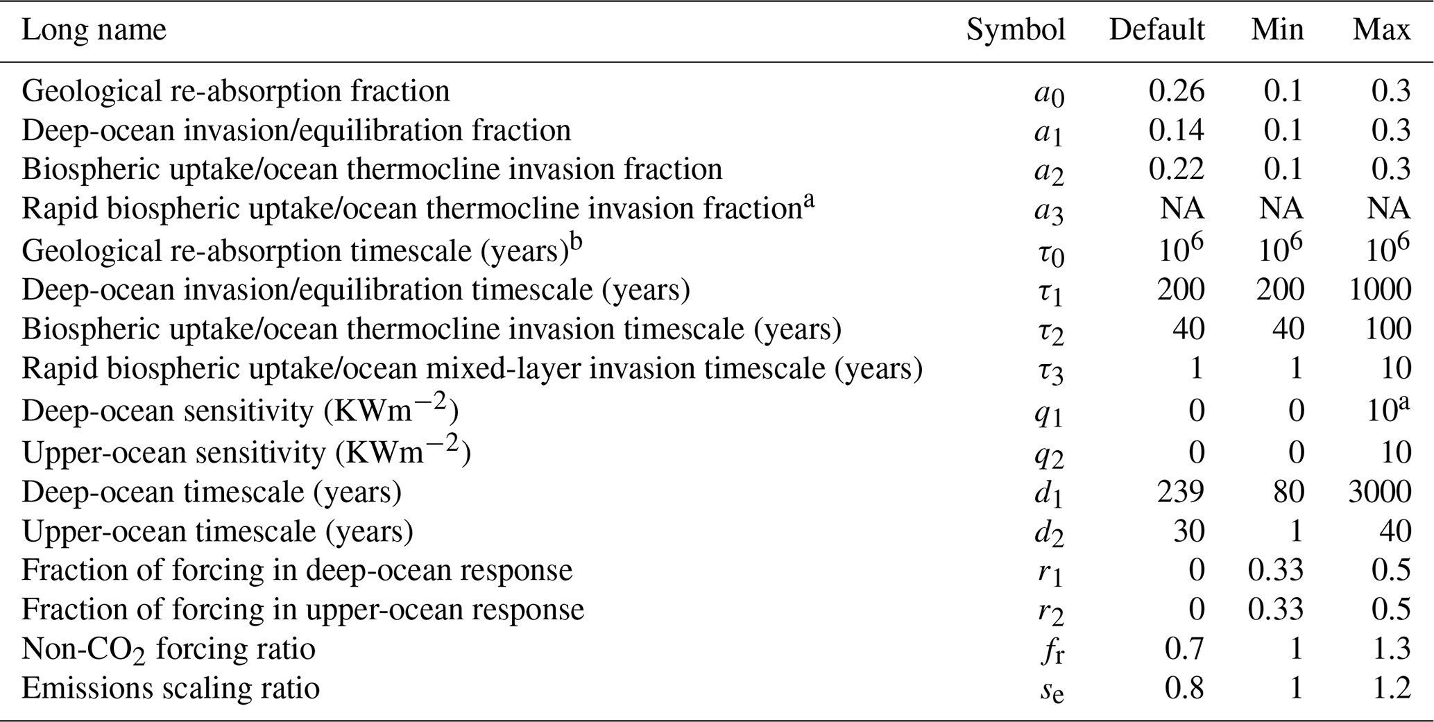
Optimization is conducted with the Goodman and Weare (2010) MCMC implementation, using flat initial parameter distributions as shown in Table 1, 200 walkers and 50 000 iterations for each optimization. Cost functions are computed for global mean temperature (T), global CO₂ concentrations (C), shallow-ocean heat content (H) and deep-ocean heat content (D):

$$\begin{array}{}\text{(12)}& {\displaystyle }\begin{array}{rl}{E}_T& =\sum _t{\left({\displaystyle \frac{\left(T\left(t\right)-T_{\mathrm{GCM}}\left(t\right)\right)}{\sqrt{\mathrm{2}}{\mathit{\sigma }}_T}}\right)}^{\mathrm{2}}{E}_C,\\ & =\sum _t{\left({\displaystyle \frac{\left(C\left(t\right)-C_{\mathrm{GCM}}\left(t\right)\right)}{\sqrt{\mathrm{2}}{\mathit{\sigma }}_C}}\right)}^{\mathrm{2}}{E}_H,\\ & =\sum _t{\left({\displaystyle \frac{\left(H\left(t\right)-H_{\mathrm{GCM}}\left(t\right)\right)}{\sqrt{\mathrm{2}}{\mathit{\sigma }}_H}}\right)}^{\mathrm{2}}{E}_D,\\ & =\sum _t{\left({\displaystyle \frac{\left(D\left(t\right)-D_{\mathrm{GCM}}\left(t\right)\right)}{\sqrt{\mathrm{2}}{\mathit{\sigma }}_D}}\right)}^{\mathrm{2}},\end{array}\end{array}$$

where σ_T represents the confidence in observed temperature values. To estimate this value, we use 2000–2019 annual global mean temperature anomalies from 1850 to 1900 in the HadCRUT-CW 100 member observational ensemble, where σ_T is the standard deviation of 2000 point (20 years, and 100 ensemble members), which represents uncertainty due to both natural variability and observational processing uncertainties (Cowtan and Way, 2013; Cowtan et al., 2015).

For σ_C, we lack an unforced standard deviation estimate, so a normalization constant of σ_C=0.3 ppm was chosen empirically to produce a ±1 ppmv range in 2016 observed concentrations in the posterior distribution (though uncertainties in emissions are much larger, and represented with the emissions scaling parameter s_e).

Shallow- and deep-ocean heat uptake (in cases where they are used) is taken as the 0–300 and 300 m+ heat content respectively in Zanna et al. (2019), with σ_H and σ_D taken as 1850–1950 standard deviations from the same dataset. Confidence estimates in these time series are not available, so σ_H and σ_D nominally represents uncertainty due to natural variability; so “C, T, heat” results should be considered to be an idealized estimate of how ocean heat information could constrain models if we were confident in that information.

In the “C, T constraint” case, optimization is conducted using −E_T and −E_C as log likelihoods in the MCMC optimizer, with parameter boundaries as listed in Table 1. The “C, T, heat constraint” case uses the sum of −E_T, −E_C, E_D and −E_H cost functions. The “C, T, paleo” case is implemented using the likely value and upper bound on Earth system sensitivity from Goodman and Weare (2010) as the median and 90th percentile of a gamma distribution for equilibrium climate sensitivity. The “C, T, RWF” constraint is implemented using a log-normal prior on transient climate response with 5–95 percentiles of 1.0–2.5 K as in Millar et al. (2017c) and a Gaussian prior on RWF (realized warming fraction, the ratio between ECS and TCR, transient climate response) with a mean of 0.6 and 5th and 9th percentiles of 0.45 and 0.75. The emissions scaling parameter is subject to Gaussian prior, which was adjusted such that uncertainty in 5 %–95 % cumulative CO₂ emissions in 2016 reflects observational uncertainties. It was found empirically that a Gaussian prior with a mean scaling parameter of 1, and standard deviations of 0.1 well represented published uncertainties, largely attributable to uncertain land use emissions (Le Quéré et al., 2018; Millar and Friedlingstein, 2018) (see Supplement Fig. S3).

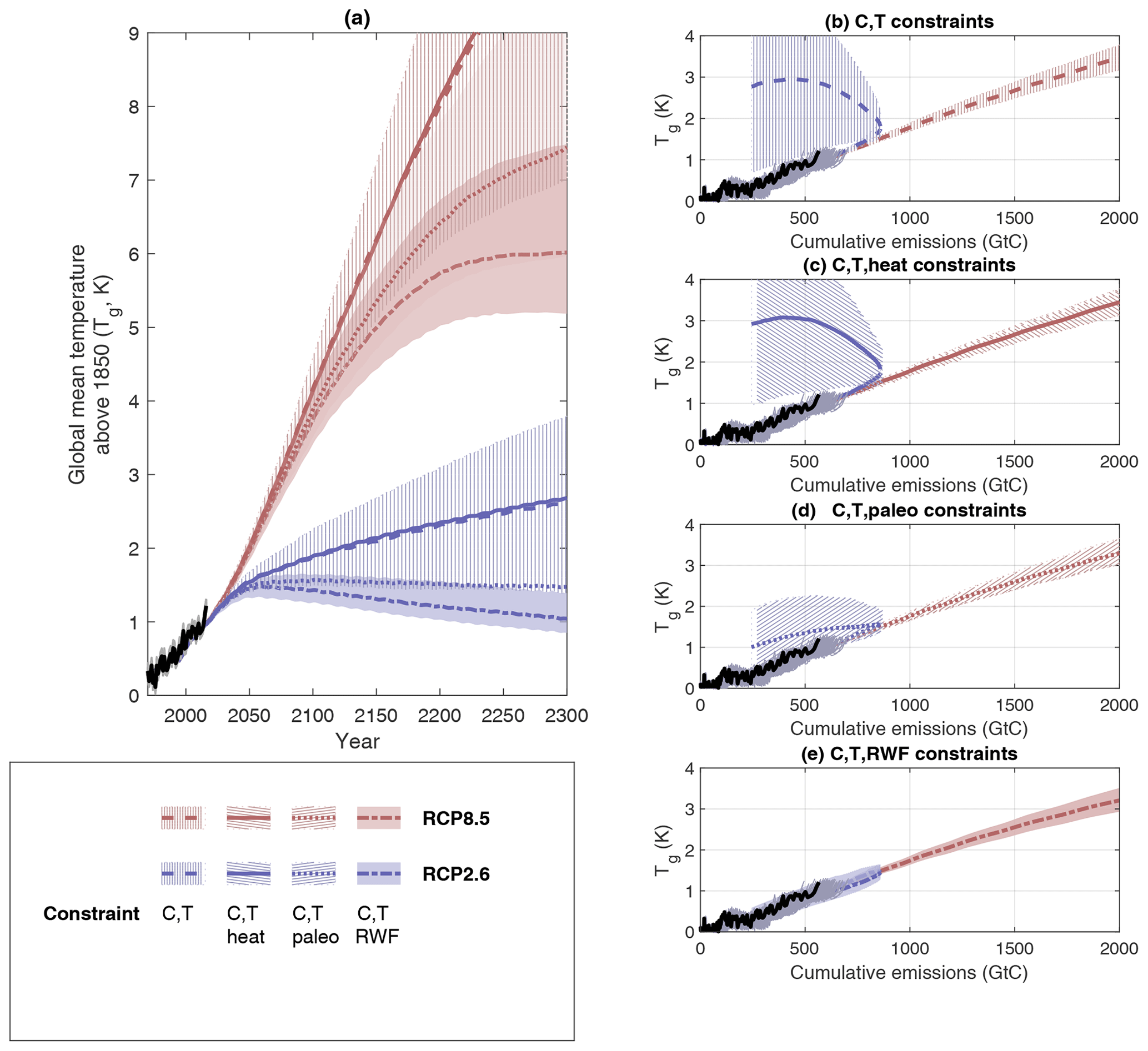
Figure 1 Posterior distributions of future global mean temperature projections constrained by 1850–2016 historical temperatures in a range of scenarios, priors and structural choices as a function of (a) time and (b–e) cumulative emissions of carbon (with 1000 years of climate evolution plotted from 1851 to 2850). Colored lines represent RCP8.5 (red) and RCP2.6 (blue). Panel (b) and dashed lines in (a) show two-timescale model posterior constrained using emissions (C) and temperature (T) only; (c) and solid lines in (a) are constrained using C, T and ocean heat content (H); (d) and dot–dash lines in (a) use C, T and RWF. Panel (e) and dotted lines use constraints on C, T and a paleoclimate prior on ECS. Shaded regions indicate the 10–90th percentile range. Solid black lines show observed global mean temperature median estimate (Cowtan and Way, 2013) and most likely estimates of combined land use and fossil fuel emissions (Le Quéré et al., 2018). Grey lines show uncertainties in observed temperature–cumulative-emissions following Millar and Friedlingstein (2018).

3 Results

3.1 The impact of prior assumptions on carbon dynamics

We consider a number of different constraint assumptions on model parameters and how they influence the range of future projections under different scenarios (Fig. 1). If the model parameters are conditioned only on historical emissions and temperature (Fig. 1a, b), transient warming under continued positive emissions is well constrained, such that temperatures follow the TCRE relationship under high-emission scenario (RCP8.5, Riahi et al., 2011) emissions. However, the relationship is not robust under long-term negative emissions in a decarbonization scenario (RCP2.6, Van Vuuren et al., 2011) where some model variants in the posterior parameter distribution allow hysteresis in which temperatures continue to rise over the following centuries under a regime of net-negative emissions.

Adding information on historical deep- and shallow-ocean heat content (Zanna et al., 2019) does not significantly constrain the system (Fig. 1a, c). However, information about long-term equilibrium climate sensitivity from paleo-climate data (Royer et al., 2011; Goodwin et al., 2018b) does provide a constraint on the degree of possible hysteresis (Fig. 1d) as does the assumption of a known RWF (the fraction of present-day warming relative to equilibrium warming associated with current forcing), which is a very strong constraint on TCRE-like behavior. This prior, used in Millar et al. (2017b), produces a model configuration in which a proportional relationship between cumulative emissions–temperature is robust during both positive and negative phases of the emissions scenario (Fig. 1e).

This raises the question of the degree to which we are confident in our knowledge of the values of ECS and RWF. In Millar et al. (2017b), the RWF prior is derived from the observation that the TCR (the warming at the time of CO₂ doubling in a transient simulation where CO₂ increases by 1 % yr⁻¹) and effective climate sensitivity (EffCS) are correlated in the CMIP5 ensemble (Millar et al., 2015) (where EffCS is the estimation of equilibrium response through the linear extrapolation of temperature change as a function of net top-of-atmosphere radiative imbalance in an instantaneous CO₂ quadrupling experiment; Gregory et al., 2004).

However, the ECS, realized over a multi-century to millennial timescale, is often significantly greater than the effective climate sensitivity (Rugenstein et al., 2016; Knutti et al., 2017), and its value may not be well constrained by observed warming (Proistosescu and Huybers, 2017; Andrews et al., 2018). As such, it is not apparent that the long-term ECS in a model like Myhre et al. (2013) can be constrained by TCR (with large implications for millennial-scale temperature evolution, as seen in Fig. S16).

These prior assumptions strongly impact the range of possible behavior under strong negative emissions in RCP2.6. However, under RCP8.5, the ensembles constrained by historical temperatures show a near-linear relationship between cumulative emissions and temperature, irrespective of prior assumptions and constraints used (Fig. 1b–e, red lines); this can be broadly understood by considering that in RCP8.5, radiative forcing continues to increase at current rates and thus long-term warming is broadly a function of TCR, which is itself constrained by historical temperature evolution.

The scenarios considered here are multi-gas, with both CO₂ emissions and non-CO₂ forcers. As expected (Mengis et al., 2018), non-CO₂ forcing assumptions can alter the effective TCRE seen in transient RCP8.5 simulations and RCP2.6 projections on shorter timescales of less than a century (see Fig. S4); however, the potential for hysteresis on longer timescales is similar in multi-gas and CO₂ only experiments.

3.2 Implications for meeting Paris temperature targets

If we consider a “high-risk” world where ECS (and its relationship to TCR) is not independently constrained, corresponding to Fig. 1b, the cumulative emissions framework is not guaranteed to hold under negative emissions, and the concept of an indefinite cumulative carbon budget associated with a temperature target may not be helpful for near-term carbon mitigation planning (results for other prior assumptions are shown in the Supplement).

We illustrate this in some idealized cases, using adaptive scenarios in which emissions are adjusted in order to achieve 1.5 and 2 ^∘C climates post-2100 (similar to those considered in Sanderson et al., 2016, 2017; Goodwin et al., 2018a). The Sanderson et al. (2016) approach allows iteration of scenarios such that targets can be met in almost all cases, but the optimization is “forward looking” (in contrast to Goodwin et al., 2018a, which simulates decisions made in response to observed warming to date without perfect knowledge of the future). Here, we follow a similar strategy to Sanderson et al. (2016), where scenarios are designed using a small number of parameters which are then optimized to meet a stabilization target post-2100.

Scenarios are conducted in three phases: before 2020 is the “historical” period, where emissions follow RCP2.6 (which is broadly consistent with observations before 2020). Between 2020 and 2040, the “uninformed” period, CO₂ emissions follow one of a range of linear mitigation pathways such that 2040 CO₂ emissions are chosen at random for each scenario, ranging from 0 to 10 GtC yr⁻¹ (our focus here is on low-emission futures, and we do not consider here futures where emissions increase post-2020).

Each ensemble member uses a single parameter set drawn from the posterior distribution of models calculated during the MCMC constraint of model parameter space in Sect. 2.1.1. Emissions follow RCP2.6 from 1850 until 2020, after which CO₂ emissions are by a “pchip” spline which is fixed at a number of points, the first of which are 2010 and 2020 RCP2.6 emissions – ensuring a smooth transition from the RCP time series to the post-2020 time series. An uninformed emissions trajectory takes place from 2020 to 2040, where emissions evolve from RCP2.6 2020 levels (10.26 GtC yr⁻¹) to a 2040 emissions level drawn randomly from a uniform distribution with bounds at 0 and 10 GtC yr⁻¹.

Post-2040, in the “adaptive” period, an emission scenario is calculated iteratively to achieve temperature stabilization at a defined target post-2100, allowing for a temperature overshoot before 2100 with a large but finite lower limit on net-negative emissions capacity in line with the largest negative emissions values seen in the integrated assessment literature for 1.5^∘ temperature stabilization targets (−20 GtC yr⁻¹, IPCC, 2018). Non-CO₂ gas emissions follow RCP2.6 throughout the simulation in all cases (clearly, these scenarios should not be treated as socioeconomically plausible scenarios but rather as idealized illustrations of Earth system response to a range of forcing pathways).

Parametric control of the adaptive phase is achieved by specifying three time points (the first, tp₁, in the range 2060–2100; the second, tp₂, in the range 2101–2300; and the third, tp₃, fixed at the end of the simulation in 2764). Each time point is associated with an emissions rate which is each weakly constrained to lie in the range −40 to +10 GtC yr⁻¹. Optimization uses MATLAB's fmincon algorithm to find optimal values of tp_1,2 and Ep${}_{\mathrm{1},\mathrm{2},\mathrm{3}}$, where the model is run iteratively for a given physical parameter set to find a solution which minimizes the RMSE from the desired annual mean global mean temperature time series target (1.5 or 2.0 ^∘C, in this case) over the date range 2100–2500.

Figure 2 Plots showing idealized pathways to 1.5 or 2.0 ^∘C temperature stabilization for an ensemble of coupled carbon–climate model configurations. Panel (a) shows the global mean temperature as a function of time for 1.5 and 2.0 ^∘C stabilization ensembles; (b) shows emissions in the historical, uniformed and adaptive stages of the simulation; (c) shows the global mean temperatures above 2006–2016 (left/right axis) levels as a function of post-2010 cumulative CO₂ emissions, while (d) shows the cumulative carbon emissions total for ensemble members as a function of time. Shaded regions in (a, b, d) indicate 10th–90th percentile range of the ensemble distribution, while dotted lines shown the 50th percentile. Gray/blue/black areas refer to uninformed/adaptive for 2.0 ^∘C/adaptive for 1.5 ^∘C respectively. Box–whisker plots in (c) show the long-term cumulative carbon budget assessed in 2100 for 1.5 and 2.0 ^∘C stabilization from 1850 to 2500. Box–whisker plots in (d) show the TCRE estimate of carbon budget with (median shown by “+”) and without (median shown by “x”) non-CO₂ gas correction. Red circle shows ensemble mean warming and post-2010 cumulative emissions in 2020.

The temperature trajectories are illustrated in Fig. 2a. Each member of the posterior distribution of possible simple climate models in Fig. 1a, b is then paired with a random 2020–2050 emissions reduction pathway, and then a post-2050 emissions pathway is calculated to optimize for stabilization at 1.5 or 2^∘ post-2100. This framework allows us to consider what would be required for long-term stabilization in a model configuration where the cumulative emissions–temperature relationship does not necessarily hold.

The resulting scenarios are idealized, some requiring a very rapid switch to large net-negative values after 2040 in order to stabilize temperatures at 1.5 ^∘C (Fig. 2b), and such rapid decarbonization may not be achievable in reality (Sanderson et al., 2016), but we can learn some useful properties of the system response by studying the relationships between near-term and long-term emissions commitments. Non-CO₂ emissions remain at RCP2.6 levels in all cases (though the non-CO₂ forcing varies as a function of the f_r parameter).

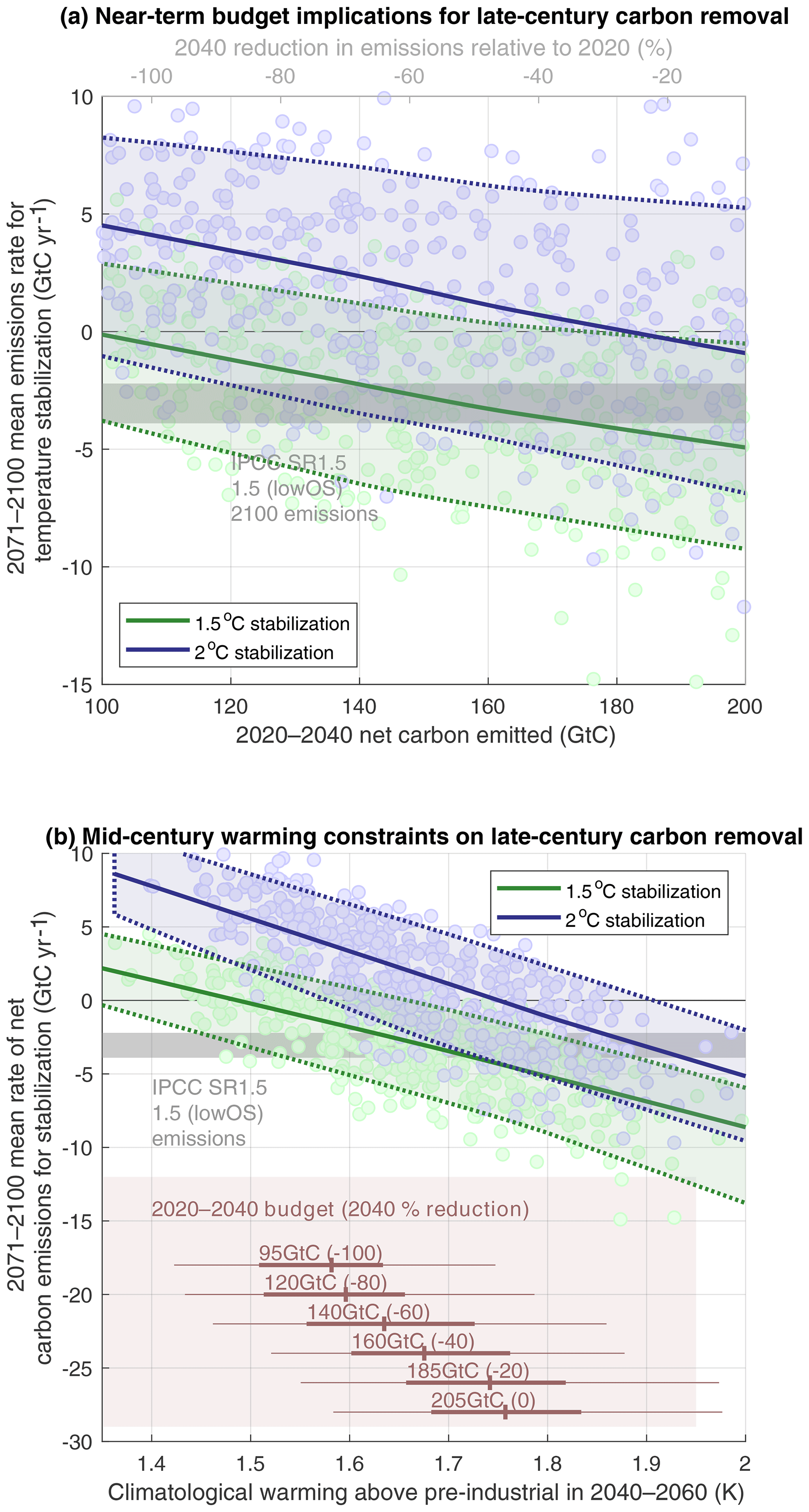
Figure 3 Plots showing (a) the relationship between mid-century cumulative carbon budgets and (b) mid-century warming and associated likelihoods of long-term carbon removal requirements for temperature stabilization. Panel (a) shows the ensemble relationship between the net carbon emitted between 2020 and 2040 (uninformed period in Fig. 1) and the associated range of possible carbon removal required later in the century in the adaptive phase for 1.5 ^∘C (green) and 2.0 ^∘C (blue) stabilization. Filled circles represent an individual ensemble member, while shaded blue/green areas represent a moving estimate of the 10–90th percentile range of the 2.0 ^∘C/1.5 ^∘C distribution (solid blue/green lines are 2.0 ^∘C/1.5 ^∘C median). Panel (b) shows 2050–2100 allowable carbon budget as a function of 2050 warming above pre-industrial levels. Dots and shading show ensemble distribution as in (a). Horizontal box–whisker plots show 10th, 25th, 50th, 75th and 90th percentiles of 2050 warming consistent with labeled 2020–2040 carbon budgets and the associated percentage reduction in 2040 emissions relative to 2020. Gray bar shows the range of reference 2100 net carbon budgets considered for end-of-century 1.5^∘ overshoot scenarios in the IPCC spacial report on 1.5^∘ (IPCC, 2018).

The range of long-term emission trajectories for temperature stabilization is diverse (Fig. 2c), in some cases requiring large negative emissions in the latter half of the 21st century to achieve temperature stabilization after 2100 (Fig. 2a). The cumulative carbon budget plume allows for a 1.5 ^∘C (2.0 ^∘C) post-2010 budget of −300 to 400 GtC (0 to 900 GtC) by 2100, a budget which continues to grow more uncertain over the centuries which follow (Fig. 2c, d). Most of the 1.5 ^∘C simulations overshoot the target in the latter half of the 21st century (Fig. 2a), and the post-2010 budget for initial exceedance of 1.5 ^∘C is more tightly constrained at 250–400 GtC (most 2 ^∘C simulations do not significantly overshoot).

This large uncertainty in the face of long-term stabilization scenarios draws into question the utility of an indefinite carbon budget (in the case where we have no prior information on equilibrium response). We can consider to what degree we can constrain future response using a definite budget with a 2020–2050 timeframe (Fig. 3). Firstly, even in the face of possible hysteresis of temperature as a function of cumulative carbon emissions, there is a linear relationship between 2020 and 2040 budgets and associated late-century carbon removal rates required for stabilization (Fig. 3a).

For example, if a late-century net carbon emission of −2.9 GtC yr⁻¹ is assumed for the late century (corresponding to the central estimate of 1.5^∘, low-overshoot stabilization from the IPCC Special Report on 1.5 ^∘C warming; IPCC, 2018), a 50 % chance of 1.5^∘ requires a 2020–2040 budget of 150 GtC, which would require a 60 % cut in emissions from present-day levels by 2040. A 75 % chance of meeting the target would require a 2020–2040 budget of 100 GtC, requiring just over 100 % cut in carbon emissions by 2040.

Here again, the choice of prior constraint on model parameters has an important effect. If the paleoclimate or RWF is used, a 75 % chance of 1.5^∘ given an assumed −2.9 GtC yr⁻¹ late-century removal rate would allow a 160 GtC (or 220 GtC) budget from 2020 to 2040 (see Fig. S14c, d). Similarly, estimated carbon budgets become more consistent with TCRE-derived estimates if an RWF prior is used, with 2100 budgets of 120–430 GtC (500–900GtC) for 1.5 ^∘C (2.0 ^∘C). This can be compared with the IPCC SR1.5 assessment of 115–230 GtC (320–550 GtC) respectively, which includes uncertainties in non-CO₂ emissions and forcings and long-timescale carbon cycle feedbacks.

These findings support the framing of emissions policy in terms of near-term emissions reductions rather than indefinite carbon budgets (Rogelj et al., 2019b). By the mid-21st century, observed warming will provide a good indication of the degree of negative emissions required for stabilization – as the average realized warming in 2040–2060 provides quite a strong constraint on budgets for the latter half of the century (Fig. 3b). The degree of possible mid-century warming can be reduced by minimizing the 2020–2040 carbon budget, but there still exists uncertainty due to the degree of thermal inertia in the system as greenhouse gas concentrations stabilize.

The strong relationship between mid-century warming and late-century carbon removal requirements for 1.5 or 2.0 ^∘C stabilization occurs because 2040–2060 warming can be potentially decreased either by fortuity (with a small value of real-world equilibrium climate sensitivity) or by action (by minimizing near-term emissions), both of which reduce late-century net carbon removal requirements. Conversely, high climate sensitivity or slow decarbonization would both result in greater mid-century warming and greater necessity for negative emissions deployment.

4 Discussion

Recent climate policy discussions have been framed in the context of a carbon budget, an allowable net total of cumulative emissions which are consistent with a desired limit on planetary warming (Allen et al., 2009; Millar et al., 2016). Nuances in the estimation of this budget have been noted relating to bias correction of existing models (Millar et al., 2017a), the compensation for the effects of non-CO₂ anthropogenic emissions (Rogelj et al., 2015a; MacDougall et al., 2015; Mengis et al., 2018) and the need for additional carbon fluxes for temperature stabilization after net-zero emissions have been achieved (Rogelj et al., 2016b; Jones et al., 2019; Mengis et al., 2018). These factors are deemed to be corrections to the TCRE-computed carbon budgets (Rogelj et al., 2019a), and values of TCRE informed by a combination of model response historical records of global surface temperatures (Gillett et al., 2013; Steinacher and Joos, 2016) form the basis for published model estimates on carbon budgets for temperature stabilization (Matthews et al., 2017a, a).

It has been noted before that at any given time, the TCRE can be expressed as a product of three components: the dependence of surface warming on radiative forcing, the fractional dependence of radiative forcing on atmospheric CO₂ and the dependence of atmospheric CO₂ on carbon emissions (Goodwin et al., 2015) – but each of these elements can potentially evolve in time as feedbacks are realized on different timescales (Rogelj et al., 2019a; Goodwin et al., 2018a). This has been addressed by introducing “threshold avoidance budgets” and “threshold exceedance budgets” (Rogelj et al., 2016b), which differ due to the lag of peak temperatures after net-zero emissions have been achieved as slower timescale components of the system equilibrate or due the effects of non-CO₂ forcers. But the scale of these effects is generally assumed to be small – on the order of 1–2 decades (Ricke and Caldeira, 2014; Zickfeld and Herrington, 2015). Idealized experiments to assess zero-emission warming commitment (MacDougall et al., 2020) in both EMICs and ESMs suggest the ZEC is small on a 50-year timescale but uncertain on a century timescale, with a large diversity of magnitude, sign and rate of warming post-cessation of emissions.

It has also been demonstrated that effective climate sensitivity likely evolves in time (Goodwin, 2018; Rohling et al., 2018), which will influence TCRE (Goodwin et al., 2015) and thus carbon budgets for a given temperature target (Goodwin et al., 2018b); thus attempts to quantify fixed real-world estimates for TCRE or effective climate sensitivity must be qualified for long timescales (Rugenstein et al., 2019) or extended net-negative emissions (Ehlert and Zickfeld, 2018). In this study, the pulse response formulation allows for the idealized separation of process response both in the evolution of atmospheric CO₂ in response to emissions and in the thermal response of the system to forcing, allowing an illustration of how prior assumptions impact feedbacks on different timescales. Future work should consider further how these fixed parameters of the carbon–climate system can be further independently constrained and integrated with the existing understanding of time-evolving net climate feedbacks.

We find that the pulse response model is not constrained to follow TCRE-like behavior without prior knowledge of equilibrium climate sensitivity. Considering other simple models, such priors are often used (either explicitly or implicitly). The parameters of the FAIR (Millar et al., 2017c; Smith et al., 2018) simple climate model, for example, are constrained using a prior on RWF (whereas projected uncertainty ranges using other models such as Goodwin et al., 2018b use no such prior). The constraint in FAIR is justified with an observed relationship between effective climate sensitivity and TCR in CMIP (Coupled Model Intercomparison Project) models and is thus likely overly constraining on possible model behavior consistent with state-of-the-art general circulation models (GCMs; see Supplement Sect. S1).

Other models do not explicitly constrain RWF but do constrain equilibrium climate sensitivity. The WASP model (Goodwin et al., 2015; Goodwin, 2016) considers multiple timescales of response and a geological prior on equilibrium warming response to emissions, which acts to preclude the possibility of strong hysteresis in the temperature response to cumulative emissions. Another simple model, HECTOR (Hartin et al., 2015), has a thermal component with a fixed climate feedback (an explicitly defined parameter in the model). Thus, irrespective of how the parameters are constrained, the model has a strong structural constraint which prevents the separation of the slow and fast response of the Earth system, which in practice would constrain the model's ZEC to small values and limit the potential for hysteresis.

In another common simple model, MAGICC (Meinshausen et al., 2011a), non-stationary feedbacks are represented in two ways – using an allowance for an oceanic surface and land surface feedback strengths, as well as having forcing-dependent feedback strengths. However, ECS values calculated using MAGICC when calibrated as an emulator of CMIP GCM simulations remain very close to the effective climate sensitivities of the target model (Meinshausen et al., 2011a), even though in some cases we know that the true ECS realized in millennial time frames is significantly greater than the EffCS value (Rugenstein et al., 2019). This requires further research but is possibly explained by the consensus that multiple feedback timescales arise from warming patterns associated with shallow- and deep-ocean warming (Li et al., 2013; Geoffroy et al., 2013). Representing feedbacks as a function of the warming of the ocean surface warming is therefore a strong structural assumption which may not capture this effect.

Recent work has made clear that the long-timescale response of the Earth system is not well constrained by past observations (Proistosescu and Huybers, 2017; Andrews et al., 2018), drawing into question whether recent transient warming is able to constrain equilibrium climate sensitivity (Otto et al., 2013) or the realized warming fraction (Millar et al., 2015). In the absence of these constraints, we cannot rule out without additional data that the slow timescale response of the Earth system associated with deep-ocean warming may lead to a world which exhibits a (relatively) low TCR but a high ECS realized over centuries or millennia (Rugenstein et al., 2019) which, as we show here, may complicate the use of an indefinite carbon budget for temperature targets.

Here, we find that these factors result in large uncertainties on remaining carbon budgets until 2100, with the possibility of hysteresis unless prior information is assumed on the value of ECS or RWF (Fig. S10). Using an RWF prior, carbon budgets for 1.5 and 2 ^∘C are broadly consistent with TCRE-derived estimates in Rogelj et al. (2018), but removing this prior reduces the lower bound of the budget from positive 120 GtC with a RWF prior (as assessed in 2100 for 1.5 ^∘C stabilization) to negative 300 GtC if the prior is removed. These factors are in addition to existing uncertainties arising from non-CO₂ forcing and scenario assumptions (approximately ±200 GtC in long-term budgets) and uncertainties in pre-industrial temperatures (approximately ±100 GtC in long-term budgets) (Rogelj et al., 2018).

Other sources of information exist which may yet resolve the uncertainty. Independent information to constrain ECS from paleoclimate (Royer et al., 2011) or process understanding (Sherwood et al., 2014; Zhai et al., 2015; Tian, 2015; Tan et al., 2016; Cox et al., 2018) may help constrain the potential for temperature hysteresis. But many constraints to date have considered only effective climate sensitivity (Gregory et al., 2004), whereas it is increasingly clear that both the timescale and amplitude of climate feedbacks need to be constrained in order to understand the Earth system response to future forcing pathways (Armour et al., 2013). Such avenues could and should be explored further.

The pulse response model of the type used here is also a simplification of global response, albeit a commonly used one (Joos et al., 2013), which resolves the degrees of freedom in the range of responses exhibited in physical Earth system models. The anthropogenically forced warming in 2040–2060 would be subject to internal variability of the order of 0.1 ^∘C (Dai et al., 2015; Rogelj et al., 2017; Kay et al., 2015) which could potentially be improved with detection approaches (Haustein et al., 2017). As such, observed mid-century warming would be of some value in constraining negative emissions requirements later in the century, which spans nearly 0.6 ^∘C over the ensemble range (Fig. 3b).

Clearly, the models used here are idealizations. Emission rates and rates of change are not constrained by technological or societal limitations, and only CO₂ pathways are modified from the RCP2.6 scenario, and so results are only illustrative of how the Earth system might respond to different hypothetical pathways. Finding pathways for technology and a policy which can actually achieve these pathways is a question for integrated assessment models. However, the present standard approach of producing scenarios through forward-looking solvers (O'Neill et al., 2016) is unable to capture the risk highlighted here associated with actors who act today with imperfect knowledge about future technology (Fuss et al., 2014; Anderson and Peters, 2016) and Earth system response. This has led to a call to frame policy in terms of near-term emissions which are compatible with projected peak levels of warming (Rogelj et al., 2019b).

The results of this study support this logic. Even in the presence of large uncertainty on long-term response to emissions, near-term climate policy can be well posed through the use of a time-limited net carbon budget or, equivalently, a near-term commitment for a percentage reduction in emissions by a certain date (Sachs et al., 2016; Oshiro et al., 2018). Observed warming over the coming decades will provide additional information on our commitments to implement negative emissions infrastructure for temperature stabilization – commitments which may or may not prove feasible to realize. But a near-term budget would provide decision makers with the tools to assess the risk of failure to meet temperature targets as a function of clearly defined targets for near-term decarbonization.