Emulating Earth system model temperatures with MESMER: from global mean temperature trajectories to grid-point-level realizations on land

Earth system models (ESMs) are invaluable tools to study the climate system's response to specific greenhouse gas emission pathways. Large single-model initial-condition and multi-model ensembles are used to investigate the range of possible responses and serve as input to climate impact and integrated assessment models. Thereby, climate signal uncertainty is propagated along the uncertainty chain and its effect on interactions between humans and the Earth system can be quantified. However, generating both single-model initial-condition and multi-model ensembles is computationally expensive. In this study, we assess the feasibility of geographically explicit climate model emulation, i.e., of statistically producing large ensembles of land temperature field time series that closely resemble ESM runs at a negligible computational cost. For this purpose, we develop a modular emulation framework which consists of (i) a global mean temperature module, (ii) a local temperature response module, and (iii) a local residual temperature variability module. Based on this framework, MESMER, a Modular Earth System Model Emulator with spatially Resolved output, is built. We first show that to successfully mimic single-model initial-condition ensembles of yearly temperature from 1870 to 2100 on grid-point to regional scales with MESMER, it is sufficient to train on a single ESM run, but separate emulators need to be calibrated for individual ESMs given fundamental inter-model differences. We then emulate 40 climate models of the Coupled Model Intercomparison Project Phase 5 (CMIP5) to create a “superensemble”, i.e., a large ensemble which closely resembles a multi-model initial-condition ensemble. The thereby emerging ESM-specific emulator parameters provide essential insights on inter-model differences across a broad range of scales and characterize core properties of each ESM. Our results highlight that, for temperature at the spatiotemporal scales considered here, it is likely more advantageous to invest computational resources into generating multi-model ensembles rather than large single-model initial-condition ensembles. Such multi-model ensembles can be extended to superensembles with emulators like the one presented here.

1 Introduction

The range of simulated climate responses to external radiative forcing is affected by both internal variability and inter-model differences (Hawkins and Sutton, 2009; Deser et al., 2012; Taylor et al., 2012). While inter-model uncertainty is typically accounted for by considering simulations from several climate models (Meehl et al., 2007; Taylor et al., 2012; Eyring et al., 2016), uncertainty due to internal climate variability is often quantified by running the same climate model a number of times with slightly different initial conditions (Deser et al., 2012; Fischer et al., 2013; Kay et al., 2015; Leduc et al., 2019).

As climate model ensembles are inherently expensive to run, there is an interest in approximating Earth system model (ESM) output with computationally cheap emulators. In the field of climate science, the term emulator is used for a variety of statistical models which learn from existing runs of complex climate models to infer properties of runs which have not been generated yet. This makes it possible to explore the phase space at a lower computational cost. ESM emulators target different aspects of the climate system. For example, some emulators focus on the impacts of sub-grid-scale parameterizations (Rougier et al., 2009; Williamson et al., 2013). Others target the effect of greenhouse gas emission scenarios on global mean temperature (Meinshausen et al., 2011; Goodwin, 2016) or on regional mean climate fields (Santer et al., 1990; Tebaldi and Arblaster, 2014; Tebaldi and Knutti, 2018). There are also emulators for regional-scale internal climate variability (Castruccio and Genton, 2016; Alexeeff et al., 2018; Link et al., 2019). Recently, the first attempts have been made to emulate the full dynamics of simple general circulation models (Scher, 2018; Scher and Messori, 2019).

In this study, the term emulator is used to refer to a computationally cheap statistical tool which generates additional realizations of land temperature field time series for a specific greenhouse gas emission pathway at a yearly resolution. The presented emulator thus produces realizations which closely resemble initial-condition ensemble members of the considered ESMs. In the context of large multi-model ensembles, our computationally cheap emulator can be used to produce look-alikes of large initial-condition ensembles for every model within the multi-model ensemble, resulting in a “superensemble”, i.e., a large ensemble which closely resembles a multi-model initial-condition ensemble.

To build this statistical temperature emulator, an overarching modular framework is proposed and put into the context of previous work in Sect. 2. The employed data and terminology are described in Sect. 3, and the specific implementation of the framework is introduced in Sect. 4. To visualize the characteristics and capabilities of the emulator, detailed results are shown for four example ESMs in Sect. 5, before applying the emulator to the large CMIP5 (Coupled Model Intercomparison Project Phase 5; Taylor et al., 2012) multi-model ensemble containing 40 climate models in Sect. 6. In Sect. 7, the results are discussed, and finally, in Sect. 8, the conclusions and an outlook are provided.

2 A framework for end-to-end climate model emulation

We propose an additive framework for temperature emulation at the yearly scale for a specific greenhouse gas emission pathway, which can be summarized as

$$\begin{array}{}\text{(1)}& T_{s,t}=f\left(T_t^{\mathrm{glob}}\right)+{\mathit{\eta }}_{s,t},\end{array}$$

where the local temperature T_s,t at grid point s and time t is defined as a response to the global mean temperature $T_t^{\mathrm{glob}}$, indicated by the function f(), and a stochastic local residual temperature variability term η_s,t. Contributions from physical feedbacks other than the ones captured within the global mean temperature signal are thus neglected. The assumption of an underlying additivity is in line with frequently employed approaches in uncertainty analysis in climate science (Hawkins and Sutton, 2009) and in climate change detection and attribution studies (Allen and Stott, 2003).

Our framework requires three modules: a global mean temperature module, a module for the grid-point-level temperature response to the global mean temperature, and a local residual temperature variability module. In the following, we place existing literature within these modules before discussing the connections to our emulator. As this study is primarily concerned with temperature, we focus solely on this variable in our literature review. However, several of the referenced studies also treat additional variables such as precipitation (e.g., Tebaldi and Arblaster, 2014; Seneviratne et al., 2016; Wartenburger et al., 2017) or cloud cover (e.g., Osborn et al., 2016).

2.1 Global mean temperature module

Global mean temperature is often an output of computationally efficient simple energy balance climate models (Meinshausen et al., 2011; Goodwin, 2016). While such models provide an estimate of the global mean temperature trend, they do not produce interannual global mean temperature variability. To obtain an ensemble of global mean temperature variability, statistical models which account for temporal autocorrelation can be used (Brown et al., 2015).

2.2 Local temperature response module

Pattern scaling is a frequently employed approach to relate local temperature to global mean temperature and is also used to emulate warming patterns across emission scenarios (Santer et al., 1990; Mitchell, 2003; Tebaldi and Arblaster, 2014). It was originally introduced by Santer et al. (1990), and different implementations exist (Mitchell, 2003). Most often, temperature fields are averaged over a late 21st century multi-decadal time period and the associated average global mean temperature is obtained (Tebaldi and Arblaster, 2014). This pattern is then linearly interpolated to a desired global mean temperature. An alternative is to extract the pattern from a transient simulation at the time when the simulation reaches the desired global mean temperature (Herger et al., 2015; Seneviratne et al., 2016; King et al., 2017). Other approaches include carrying out a linear regression (Lynch et al., 2017) or fitting a linear mixed-effect model (Alexeeff et al., 2018) to global mean temperature at each grid point individually. The most important assumption underlying pattern scaling is that local mean temperatures are linearly related to global mean temperature and that this relationship is consistent across forcing scenarios. For surface temperature on land this assumption is satisfactorily met (Mitchell, 2003; Tebaldi and Arblaster, 2014; Seneviratne et al., 2016; Wartenburger et al., 2017; Osborn et al., 2018). However, for strong mitigation scenarios and under strong aerosol forcing, pattern scaling is less accurate (May, 2012; Levy et al., 2013). Additionally, it is assumed that external forcing and internal variability are independent, which may not always be true (Lopez et al., 2014).

More complex local response emulation methods are rare and often directly conditioned on CO₂ concentration profiles instead of global mean temperature (Castruccio et al., 2014; Holden and Edwards, 2010). For instance, it has been proposed to employ past trajectories of atmospheric CO₂ to model regional temperatures with an infinite distributed lag model to capture nonlinear behavior in spatial patterns for regional-scale emulation (Castruccio et al., 2014) and within global space–time models (Castruccio and Stein, 2013). Other authors use singular value decomposition to emulate decadal temperature fields across scenarios while accounting for complex spatiotemporal feedbacks (Holden and Edwards, 2010; Holden et al., 2014).

While the focus is usually on emulating the pattern associated with the global mean temperature trend, patterns associated with physical modes of variability such as the El Niño–Southern Oscillation and the Pacific Decadal Oscillation can additionally be derived (McKinnon and Deser, 2018).

2.3 Local residual temperature variability module

Several approaches exist to emulate local residual temperature variability based on observations and climate model simulations (Castruccio and Stein, 2013; Osborn et al., 2016; McKinnon et al., 2017; Alexeeff et al., 2018; Link et al., 2019). Observations can be employed to avoid climate model biases but are limited by rather short observational records when deriving the local temperature variability properties (Osborn et al., 2016; McKinnon et al., 2017; McKinnon and Deser, 2018). The simplest approach is to detrend observed temperature time series and obtain additional realizations by shifting the starting date of the time series (Osborn et al., 2016). More realizations have been generated by resampling the spatial fields of detrended observed local temperature variability in blocks of 2 years (McKinnon et al., 2017). The approach was later refined to explicitly account for physical modes of variability to further reduce temporal autocorrelation in the resampled fields (McKinnon and Deser, 2018).

When employing ESMs instead, longer time series and multiple realizations are available to derive the statistical properties of the local residual temperature variability. Several authors fit autoregressive (AR) models to a set of climate model runs to account for temporal autocorrelation when emulating local residual temperature variability (Castruccio and Stein, 2013; Castruccio et al., 2014; Castruccio and Genton, 2016; Bao et al., 2016). Thereby, the spatial dependence in the innovation terms of the AR models can be considered by parameterizing their covariance structure with a Matérn covariance function (Castruccio and Stein, 2013; Castruccio and Genton, 2016; Bao et al., 2016). Alternatively, detrended ESM runs can be decomposed into their principal components, and their phases can be randomly perturbed to generate additional realizations of local residual temperature variability (Link et al., 2019).

All approaches listed so far rely on the assumption that local residual temperature variability is stationary in time, which is known not to be fulfilled everywhere. Olonscheck and Notz (2017) and references therein provide a comprehensive overview of possible changes in temperature variability in the historical time period and the business-as-usual greenhouse gas emission scenario for the large CMIP5 multi-model ensemble. They find that the strongest and most likely changes will occur over oceans but also point out land regions where variability is projected to change in the future. During the historical time period, they identify only weak changes in the variability. To account for such temporal nonstationarities, it has been proposed to resample the detrended temperature fields of large single-model initial-condition ensembles within a certain window size around a global mean temperature level (Alexeeff et al., 2018). To enlarge the number of fields to sample from, a method has additionally been developed to stochastically emulate spatially nonstationary Gaussian fields with a LatticeKrig model (Nychka et al., 2018).

2.4 This study

While most studies focus on one or two of the modules required to mimic an initial-condition ensemble, this study proposes a framework which incorporates all three components. Since only 12 out of 40 CMIP5 models provide several initial-condition members, it is essential to test to what extent an emulator trained on a single run is able to approximate both its training run and additional independent initial-condition members. We thus emulate the full CMIP5 multi-model ensemble based on single training runs and create a superensemble which accounts for inter-model uncertainty across all 40 climate models. To the best of our knowledge, this study is the first to implement an emulator which mimics an initial-condition ensemble based on a single training run and applies it to such a large multi-model ensemble.

3 Data and terminology

3.1 Data sources and terminology

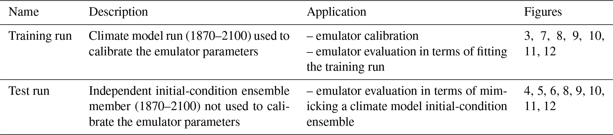
Runs from 40 CMIP5 climate models (Taylor et al., 2012) covering the historical time period (1870–2005) and the business-as-usual greenhouse gas emission scenario RCP8.5 (2006–2100; Riahi et al., 2011) are employed. To calibrate the emulator, a single run per climate model is used. This run is referred to as the training run (Table 1). For 12 out of 40 CMIP5 climate models more than one initial-condition member is available. These additional independent initial-condition ensemble members are referred to as test runs (Table 1). A special focus is on four ESMs with differing model genealogies (Knutti et al., 2013), namely CanESM2, CESM1(CAM5), HadGEM2-ES, and MPI-ESM-LR. All climate models, the associated modeling groups, and the number of initial-condition members employed here are listed in Table A1.

Table 1 Terms used to refer to different climate model runs throughout this study.

Additionally, stratospheric aerosol optical depth is used as a proxy for volcanic activity during the historical time period. This aerosol dataset was originally described by Sato et al. (1993) and later updated to cover the considered time period.

3.2 Data processing

Here, we focus on surface temperature anomaly at a yearly resolution. Temperature fields were bilinearly interpolated onto a $\mathrm{2.5}{}^{\circ }\times \mathrm{2.5}{}^{\circ }$ grid, resulting in 3043 land grid points for each climate model. Yearly mean temperatures were computed at each grid point, and the average over the reference period of 1870–1899 in the training run at the respective grid points was subtracted. In the text, for simplicity reasons, we use the term “temperature” when referring to “yearly surface temperature anomaly”. For the stratospheric aerosol optical depth, the globally averaged yearly time series is employed.

Whenever regional averages are shown, area-weighted means are referred to. The regions employed in this study are 26 land regions defined in the Special Report on Managing the Risks of Extreme Events (SREX) (Seneviratne et al., 2012) as well as global mean and global land mean (Fig. 1). While global mean refers to the average across all grid points, global land mean refers to the average across all land grid points excluding Antarctica.

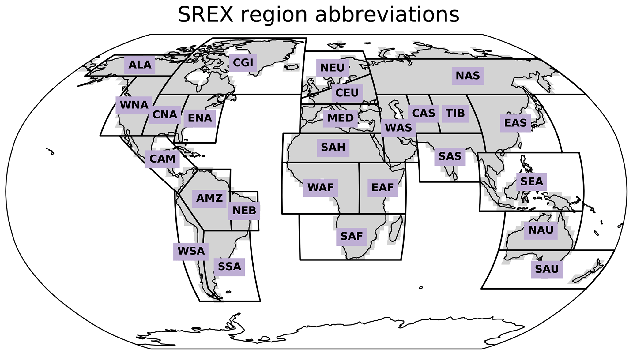
Figure 1 Map of the SREX regions and their abbreviations. The considered land grid points are shown in gray.

4 Methods

4.1 Framework implementation

4.1.1 General approach

We follow the framework introduced in Sect. 2 to emulate temperature fields at the yearly scale for a specific greenhouse gas emission pathway. The chosen implementation is called MESMER, which stands for Modular Earth System Model Emulator with spatially Resolved output, and is shown in Fig. 2. Detailed information for each individual module is provided in the following sections. In short, the global mean temperature $T_t^{\mathrm{glob}}$ is split into a trend and a variability term, both of which contribute linearly to the local temperature T_s,t. The residual local temperature variability η_s,t is modeled as an AR(1) process with spatially correlated innovations.

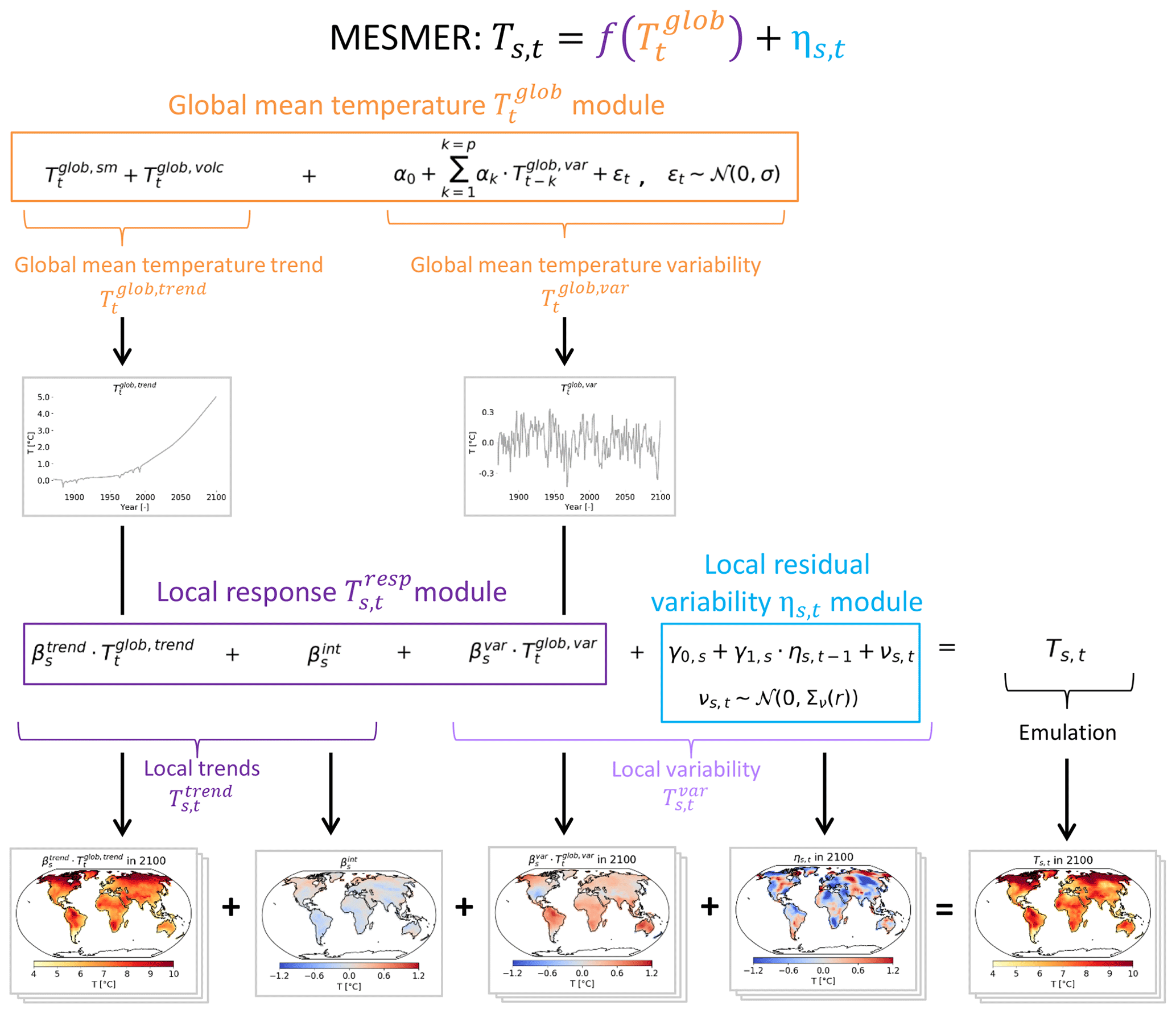
Figure 2 Illustration of the emulation framework with the MESMER implementation.

To calibrate the emulator, a single run spanning 231 years (1870–2100) per model is used. For the calibration, the global mean temperature trajectory and the associated land temperature fields are required.

4.1.2 Global mean temperature module

In the global mean temperature module, additional realizations of global mean temperature time series $T_t^{\mathrm{glob}}$ are generated. For this purpose, $T_t^{\mathrm{glob}}$ is separated into a trend $T_t^{\mathrm{glob},\mathrm{trend}}$ shared by all emulations and a variability term $T_t^{\mathrm{glob},\mathrm{var}}$ which varies between individual emulations:

$$\begin{array}{}\text{(2)}& T_t^{\mathrm{glob}}=T_t^{\mathrm{glob},\mathrm{trend}}+T_t^{\mathrm{glob},\mathrm{var}}.\end{array}$$

In $T_t^{\mathrm{glob},\mathrm{trend}}$, smooth forcing $T_t^{\mathrm{glob},\mathrm{sm}}$ and abrupt changes induced by volcanic eruptions $T_t^{\mathrm{glob},\mathrm{volc}}$ are accounted for in an additive way:

$$\begin{array}{}\text{(3)}& T_t^{\mathrm{glob},\mathrm{trend}}=T_t^{\mathrm{glob},\mathrm{sm}}+T_t^{\mathrm{glob},\mathrm{volc}}.\end{array}$$

First, $T_t^{\mathrm{glob},\mathrm{sm}}$ is derived by locally weighted scatterplot smoothing (LOWESS) of $T_t^{\mathrm{glob}}$.

In a next step, $T_t^{\mathrm{glob},\mathrm{volc}}$ is approximated as the linear response of the residuals of the smooth trend, i.e., $T_t^{\mathrm{glob}}-T_t^{\mathrm{glob},\mathrm{sm}}$, to stratospheric aerosol optical depth AOD_t with regression coefficients λ₀ and λ₁:

$$\begin{array}{}\text{(4)}& T_t^{\mathrm{glob},\mathrm{volc}}={\mathit{\lambda }}_{\mathrm{0}}+{\mathit{\lambda }}_{\mathrm{1}}\cdot {\mathit{\text{AOD}}}_t.\end{array}$$

The time series of global mean temperature variability $T_t^{\mathrm{glob},\mathrm{var}}=T_t^{\mathrm{glob}}-T_t^{\mathrm{glob},\mathrm{trend}}$ is modeled as an AR process of order p with coefficients ${\mathit{\alpha }}_{\mathrm{0}},\mathrm{\dots },{\mathit{\alpha }}_p$ such that

$$\begin{array}{}\text{(5)}& \begin{array}{rl}& T_t^{\mathrm{glob},\mathrm{var}}={\mathit{\alpha }}_{\mathrm{0}}+\sum _{k=\mathrm{1}}^{k=p}{\mathit{\alpha }}_k\cdot T_{t-k}^{\mathrm{glob},\mathrm{var}}+{\mathit{ϵ}}_t\\ & \mathrm{with}{\mathit{ϵ}}_t\sim \mathcal{N}(\mathrm{0},\mathit{\sigma }),\end{array}\end{array}$$

whereby ϵ_t is a white noise innovation term drawn from a Gaussian distribution with mean zero and standard deviation σ.

In this study, the LOWESS smoothing window length is 50 years with weights decaying with increasing distance according to a tricube weight function. The regression coefficients for the forced response to volcanic eruptions are obtained with the ordinary least squares (OLS) algorithm. The coefficients of the AR process are fit by means of maximum likelihood, and the Bayesian information criterion (BIC) is employed to select its order p with the maximum considered order being 8.

4.1.3 Local temperature response module

The local temperature response module translates the global mean temperature signal into a grid-point-level response $T_{s,t}^{\mathrm{resp}}$. Motivated by the pronounced linear scaling of regional land temperatures with global mean temperature (Seneviratne et al., 2016; Wartenburger et al., 2017), the local response is expressed as

$$\begin{array}{}\text{(6)}& \begin{array}{rl}{T}_{s,t}^{\mathrm{resp}}& =f\left(T_t^{\mathrm{glob}}\right)=f\left(T_t^{\mathrm{glob},\mathrm{trend}},T_t^{\mathrm{glob},\mathrm{var}}\right)\\ & ={\mathit{\beta }}_s^{\mathrm{trend}}\cdot T_t^{\mathrm{glob},\mathrm{trend}}+{\mathit{\beta }}_s^{\mathrm{int}}+{\mathit{\beta }}_s^{\mathrm{var}}\cdot T_t^{\mathrm{glob},\mathrm{var}},\end{array}\end{array}$$

with regression coefficients ${\mathit{\beta }}_s^{\mathrm{trend}},{\mathit{\beta }}_s^{\mathrm{int}}$, and ${\mathit{\beta }}_s^{\mathrm{var}}$, whereby ${\mathit{\beta }}_s^{\mathrm{int}}$ represents the intercept term. Hence, the responses of the local mean temperature to $T_t^{\mathrm{glob},\mathrm{trend}}$ and $T_t^{\mathrm{glob},\mathrm{var}}$ are separately taken into account.

In this study, the linear regression coefficients are estimated with OLS at each grid point.

4.1.4 Local residual temperature variability module

The local residual temperature variability η_s,t refers to the spatiotemporally correlated residual variability, which cannot be accounted for through a response to $T_t^{\mathrm{glob}}$. This variability is assumed to be Gaussian in nature (see Fig. S1 in the Supplement for the results of a Shapiro–Wilk test for normality) and stationary in time, which makes it possible to model the time series as local AR(1) processes with spatially correlated innovations (Humphrey and Gudmundsson, 2019). Hence, additional realizations of η_s,t are generated stochastically according to

$$\begin{array}{}\text{(7)}& \begin{array}{rl}& {\mathit{\eta }}_{s,t}={\mathit{\gamma }}_{\mathrm{0},s}+{\mathit{\gamma }}_{\mathrm{1},s}\cdot {\mathit{\eta }}_{s,t-\mathrm{1}}+{\mathit{\nu }}_{s,t}\\ & \mathrm{with}{\mathit{\nu }}_{s,t}\sim \mathcal{N}(\mathrm{0},{\mathrm{\Sigma }}_{\mathit{\nu }}(r\left)\right),\end{array}\end{array}$$

whereby γ_0,s and γ_1,s are the coefficients of the AR model, and ν_s,t represents spatially correlated innovations drawn from a multivariate Gaussian with mean zero and covariance matrix Σ_ν(r) (Cressie and Wikle, 2011).

For an AR(1) process, Σ_ν(r) can be analytically derived from the covariance matrix of the residual variability Σ_η(r) with

$$\begin{array}{}\text{(8)}& {\mathrm{\Sigma }}_{\mathit{\nu }}(r{)}_{i,j}=\sqrt{\mathrm{1}-{\mathit{\gamma }}_{\mathrm{1},i}}\cdot \sqrt{\mathrm{1}-{\mathit{\gamma }}_{\mathrm{1},j}}\cdot {\mathrm{\Sigma }}_{\mathit{\eta }}(r{)}_{i,j},\end{array}$$

whereby the indices i and j refer to spatial locations s (Cressie and Wikle, 2011).

To estimate Σ_η(r), the empirical covariance matrix ${\stackrel{\mathrm{̃}}{\mathrm{\Sigma }}}_{\mathit{\eta }}$ is computed. However, ${\stackrel{\mathrm{̃}}{\mathrm{\Sigma }}}_{\mathit{\eta }}$ is rank deficient because substantially fewer temperature field samples are available than there are land grid points. Thus, ${\stackrel{\mathrm{̃}}{\mathrm{\Sigma }}}_{\mathit{\eta }}$ needs to be regularized to obtain a robust estimate of the covariations between the grid points. For this purpose, we employ localization, an approach which is well established in the field of data assimilation (Carrassi et al., 2018). Localization retains anisotropy on regional scales, which is an important asset when stochastically modeling temperature variability since anisotropy is a prevalent feature due to physical factors such as the prevailing wind direction and geometry of mountainous terrain. To localize ${\stackrel{\mathrm{̃}}{\mathrm{\Sigma }}}_{\mathit{\eta }}$, it is point-wise multiplied with a smooth correlation function G(r) with exponentially vanishing correlations with distance:

$$\begin{array}{}\text{(9)}& {\mathrm{\Sigma }}_{\mathit{\eta }}\left(r\right)={\stackrel{\mathrm{̃}}{\mathrm{\Sigma }}}_{\mathit{\eta }}\circ G\left(r\right),\end{array}$$

whereby ∘ denotes the Hadamard product. Here, G(r) is the numerically efficient Gaspari–Cohn function (Gaspari and Cohn, 1999), which vanishes beyond 2 times the localization radius L:

$$\begin{array}{}\text{(10)}& G\left(r\right)=\left\{\begin{array}{l}\mathrm{1}-\frac{\mathrm{5}}{\mathrm{3}}\cdot r^{\mathrm{2}}+\frac{\mathrm{5}}{\mathrm{8}}\cdot r^{\mathrm{3}}+\frac{\mathrm{1}}{\mathrm{2}}\cdot r^{\mathrm{4}}-\frac{\mathrm{1}}{\mathrm{4}}\cdot r^{\mathrm{5}},\\ \text{if }\mathrm{0}\le r<\mathrm{1},\\ \mathrm{4}-\mathrm{5}\cdot r+\frac{\mathrm{5}}{\mathrm{3}}\cdot r^{\mathrm{2}}+\frac{\mathrm{5}}{\mathrm{8}}\cdot r^{\mathrm{3}}-\frac{\mathrm{1}}{\mathrm{2}}\cdot r^{\mathrm{4}}+\frac{\mathrm{1}}{\mathrm{12}}\cdot r^{\mathrm{5}}\\ -\frac{\mathrm{2}}{\mathrm{3}}\cdot r^{-\mathrm{1}},\\ \text{if }\mathrm{1}\le r<\mathrm{2},\\ \mathrm{0},\\ \text{if }r\ge \mathrm{2},\end{array}\right.\end{array}$$

with $r=\frac{d}{L}$ and d the geographical distance between two grid points.

In this study, the AR(1) coefficients are fit at each grid point by means of maximum likelihood. In our framework implementation, the obtained intercept terms γ_0,s are effectively zero, as the local response module already contains an intercept term (Eq. 6). The localization radius to regularize ${\stackrel{\mathrm{̃}}{\mathrm{\Sigma }}}_{\mathit{\eta }}$ is determined by cross-validation with a leave-one-out approach. Localization radii between 1000 and 4750 km every 250 km are tested. Thereby, the empirical covariance matrix is estimated based on 230 years, and the likelihood to draw the field of the left-out year from the regularized matrix is computed. This process is repeated until every year has been left out once for every localization radius. The respective log-likelihood values for each localization radius are summed up across the left-out years, and the radius which is associated with the maximum likelihood is chosen.

4.2 Evaluating the emulator

The emulator's performance is evaluated on the training run and – where available – on test runs. While the evaluation on the training run indicates how successfully this framework implementation captures the training run, the evaluation on the test runs serves as a proxy for the emulator's capability in mimicking true ESM initial-condition ensembles. For the evaluation, 1000 emulations are generated for each climate model.

4.2.1 Local trend verification

The local trends $T_{s,t}^{\mathrm{trend}}$ are shared by all emulations and serve as an estimate of the externally forced response with

$$\begin{array}{}\text{(11)}& T_{s,t}^{\mathrm{trend}}={\mathit{\beta }}_s^{\mathrm{trend}}\cdot T_t^{\mathrm{glob},\mathrm{trend}}+{\mathit{\beta }}_s^{\mathrm{int}}.\end{array}$$

To evaluate how well the emulated local trends capture true climate model runs, the Pearson correlation of $T_{s,t}^{\mathrm{trend}}$ with T_s,t of the corresponding training run is computed. For climate models with test runs, the correlation coefficient is additionally computed between $T_{s,t}^{\mathrm{trend}}$ and each test run.

4.2.2 Local variability verification

The local variability $T_{s_{,}t}^{\mathrm{var}}$ is different in each emulation and corresponds to the internally generated natural variability:

$$\begin{array}{}\text{(12)}& T_{s,t}^{\mathrm{var}}={\mathit{\beta }}_s^{\mathrm{var}}\cdot T_t^{\mathrm{glob},\mathrm{var}}+{\mathit{\eta }}_{s,t}.\end{array}$$

To compare the emulated $T_{s,t}^{\mathrm{var}}$ to true climate model runs, an estimate for the local variability within the climate models needs to be obtained. For this purpose, the emulated local trends $T_{s,t}^{\mathrm{trend}}$ (Eq. 11) are subtracted from the climate models' T_s,t.

To evaluate $T_{s,t}^{\mathrm{var}}$, on the grid-point level, lag-1 temporal autocorrelations and standard deviations are considered. Additionally, spatial cross-correlations between grid points are verified. These quantities are computed for each individual emulation as well as for all climate model runs. For each quantity, the Pearson correlation coefficient between each individual emulation and the training run is calculated. Additionally, the correlation between each individual test run and the respective training run is computed where test runs are available. These correlations between the climate model runs serve as benchmark values for the correlations between the emulations and the training run.

4.2.3 Regional-scale ensemble reliability verification

On regional scales, the emulated temperatures T_s,t (Eq. 1) are evaluated visually and quantitatively in terms of ensemble reliability, i.e., the ability to capture the distribution of ESM runs with an ensemble of emulations (Weigel, 2012). For the visual verification, regionally averaged emulated time series are compared to climate model runs for global land, Central Europe (CEU), and Southeastern South America (SSA). In the quantitative verification, the emulator's ability to reliably reproduce a set of ESM quantiles (5 %, 50 %, 95 %) is evaluated in all 27 land regions. Smooth time series of the emulated quantiles are obtained based on the 1000 emulations, and the percentage of time slots during which a climate model run is below these emulated quantiles is counted. This is done for the training run and – where available – also for the test runs. Additionally, the counting is carried out for each individual emulation. The resulting deviations of the individual emulations from the emulated quantiles can be compared to the deviation the climate model runs exhibit from the emulated quantiles. If the climate model run deviation lies within the 95 % interval spanned by the individual emulation deviations, the climate model run is considered indistinguishable from individual emulations at this quantile.

5 Exploring emulator properties for four example ESMs

5.1 Calibration results

The parameters obtained from training the emulator on four example ESMs reveal distinct inter-ESM differences in every emulator module (Fig. 3). The global mean temperature trends diverge by 0.9 ^∘C by the end of the 21st century. For each ESM, $T_t^{\mathrm{glob},\mathrm{var}}$ is described by oscillating AR coefficients with the first lag being positive, but the AR process order and the standard deviations of the innovations vary.

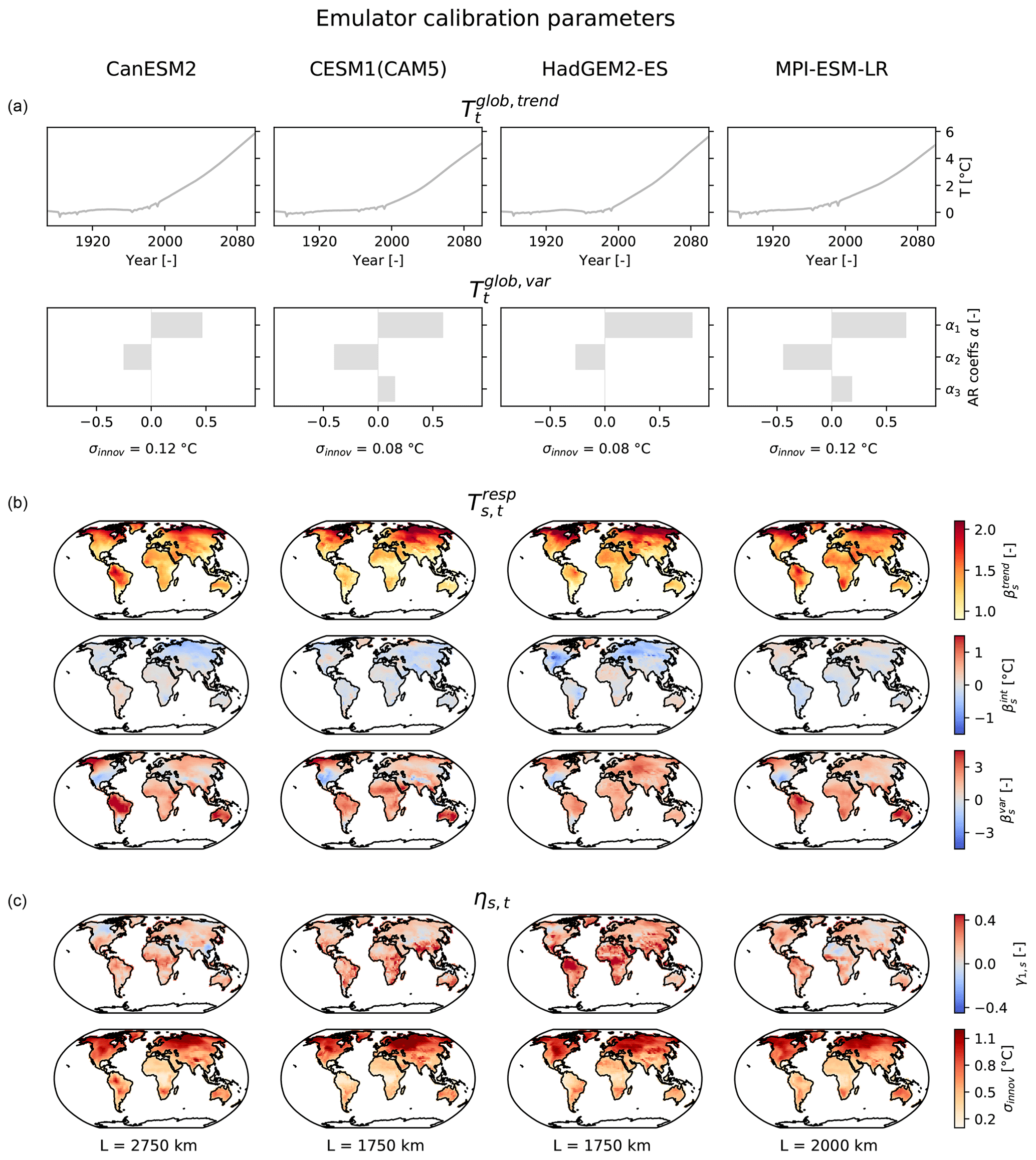
Figure 3 Emulator calibration parameters (rows) for four example ESMs (columns). (a) For the global mean temperature module, $T_t^{\mathrm{glob},\mathrm{trend}}$ and the AR coefficients plus the standard deviation of the innovations of $T_t^{\mathrm{glob},\mathrm{var}}$ are depicted. (b) For the local temperature response module, the regression coefficients are shown. (c) For the local residual temperature variability module, the lag-1 AR coefficients, the standard deviations of the innovations, and the localization radii are displayed.

In the local response module (Eq. 6), the strongest warming rates, i.e., the largest ${\mathit{\beta }}_s^{\mathrm{trend}}$ terms, are found in the northern high latitudes, but there are substantial differences in the ${\mathit{\beta }}_s^{\mathrm{trend}}$ patterns between emulators trained on different ESMs (Fig. 3). For example, the CESM1(CAM5) emulator exhibits less warming in the tropics than the others do. In all emulators, the intercept term ${\mathit{\beta }}_s^{\mathrm{int}}$ is generally small in magnitude and smooth in space. The ${\mathit{\beta }}_s^{\mathrm{var}}$ fields indicate that Alaska, the Amazon, and Australia frequently covary with global mean temperature variability. Only for HadGEM2-ES does central Asia emerge as a region of large ${\mathit{\beta }}_s^{\mathrm{var}}$ values.

The local residual variability (Eq. 7) exhibits generally less memory in the northern high latitudes than in the tropics as indicated by the lag-1 autocorrelation coefficients (Fig. 3). The innovations are largest in magnitude in high-latitude continental climates, such as northern Asia, and smallest in the tropics. However, for these quantities the patterns also differ between emulators calibrated on different ESMs. The localization radii chosen to regularize the empirical spatial covariance matrix ${\stackrel{\mathrm{̃}}{\mathrm{\Sigma }}}_{\mathit{\eta }}$ range from 1750 to 2750 km.

5.2 Example realizations

Emulated temperature fields are visually indistinguishable from ESM test runs that were not used during training (Fig. 4). All fields exhibit the strongest warming and variability in the northern high latitudes. In terms of variability, CESM1(CAM5), HadGEM2-ES, and their emulations show more patchy behavior, i.e., locally more confined variability, than CanESM2 and MPI-ESM-LR.

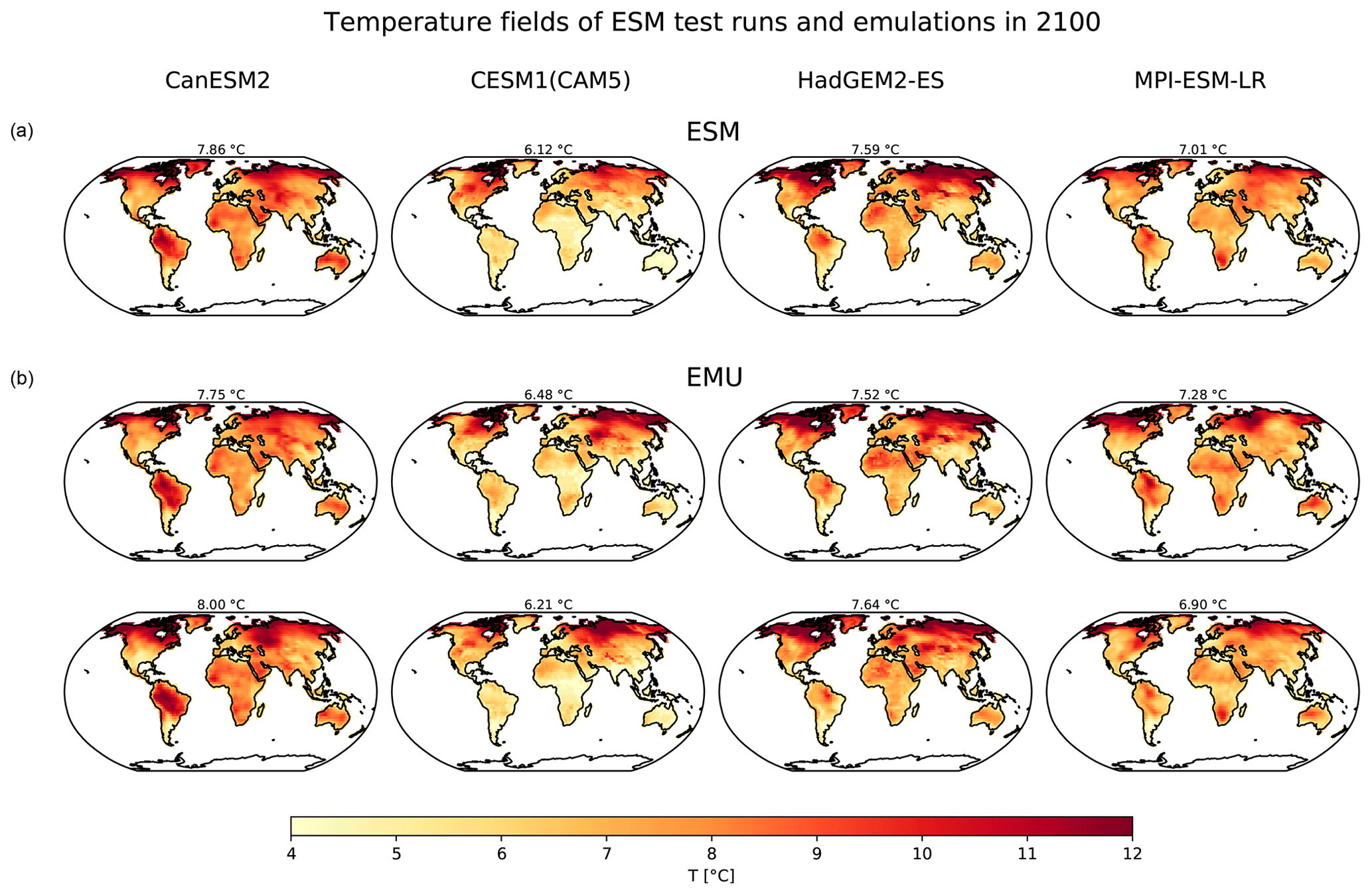
Figure 4 Temporal snapshots depicting temperature field realizations in 2100 (rows) for four example ESMs (columns). (a) One ESM field from a test run and (b) two emulations (EMUs) are shown. The temperature on top of each map refers to the global land mean.

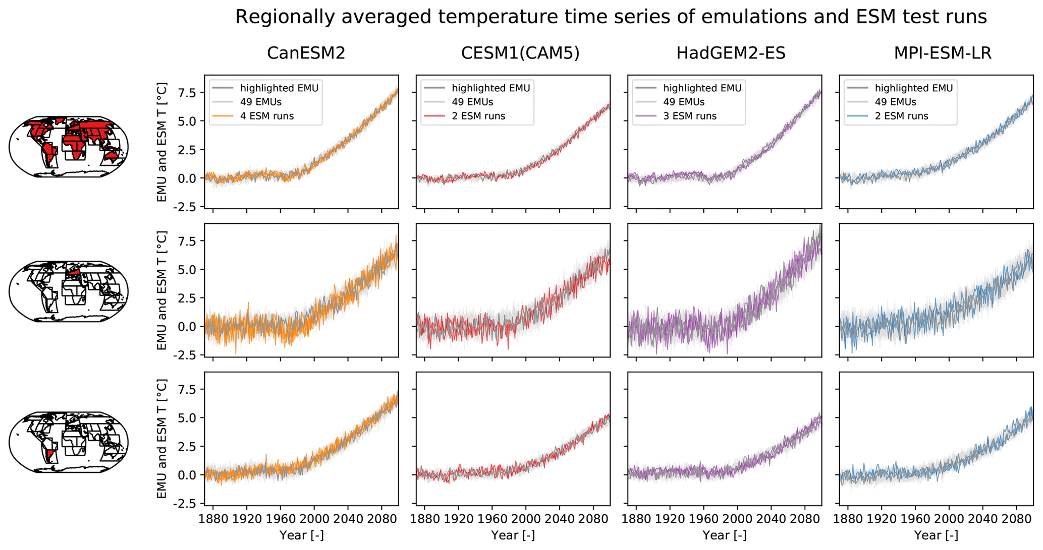
Figure 5 Regionally averaged temperature time series (rows) for four example ESMs (columns). The regions are (from top to bottom) global land, Central Europe (CEU), and Southeastern South America (SSA). In each panel, one emulation (EMU) is highlighted in dark gray and 49 other emulations are shown in light gray. Additionally, all available ESM test runs are plotted in color.

Time series of emulations and ESM test runs averaged over global land, CEU, and SSA highlight the emulators' capability to reproduce the regionally characteristic behavior of the climate system (Fig. 5). These regions differ in terms of the warming trend and variability around this trend. The variability is smallest on the global scale since local anomalies tend to average out globally. In CEU, the warming rate and the variability are larger than in SSA.

5.3 Emulator transferability between ESMs

Figure 6 explicitly shows what the results of Sect. 5.1 and 5.2 have already hinted at, namely that an ensemble of emulations generated by an emulator calibrated on a specific ESM is capturing unique properties of that ESM, which in turn are not transferable to other ESMs. For example, the warming rate of the ensemble generated by the CESM1(CAM5) emulator is inconsistent with all three other ESMs on the global land scale. As expected, differences are also found in the variability around the trend, which is, e.g., visibly smaller in SSA in the CESM1(CAM5) emulations than in the runs of the other ESMs. The implications of these results are further discussed in Sect. 7.3.

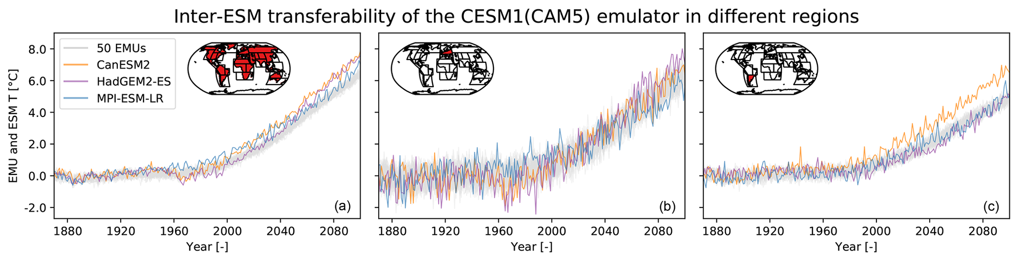
Figure 6 Time series of 50 emulations (EMUs) from the CESM1(CAM5) emulator (light gray) overlaid with runs from the three other example ESMs for three regions: global land (a), CEU (b), and SSA (c).

6 Creating a CMIP5 superensemble

6.1 Calibration results

Figure 7 shows summary statistics of the calibrated parameters for each CMIP5 climate model, highlighting inter-model differences in each emulator module. In the Supplement, plots analogous to Fig. 3 are additionally provided for each climate model for readers interested in the geographical patterns of the emulator parameters (Figs. S2–S10).

Figure 7 Emulator properties (rows) of the 40 CMIP5 climate models (columns). (a) For the global mean temperature module, $T_t^{\mathrm{glob},\mathrm{trend}}$ and the AR coefficients plus the standard deviation of the innovations of $T_t^{\mathrm{glob},\mathrm{var}}$ are depicted. (b) For the local temperature response module, the regression coefficients are shown. (c) For the local residual variability module, the lag-1 AR coefficients, the standard deviations of the innovations, and the localization radii are displayed. Box plots indicate the median (dark gray line), the interquartile range (gray box), and the full range of values (gray whiskers).

In the global mean temperature module (Eq. 2), $T_t^{\mathrm{glob},\mathrm{trend}}$ ranges between 3.4 and 6.3 ^∘C at the end of the 21st century (Fig. 7). For 45 % of the climate models, $T_t^{\mathrm{glob},\mathrm{var}}$ can be modeled as an AR(1) process. In the remaining ones either an AR(2) or AR(3) process is chosen. All emulators contain oscillating positive and negative AR coefficients with the first coefficient being positive, but they differ in the magnitude of the respective AR coefficients. The associated innovations vary in their standard deviations by a factor of almost 3 (0.06–0.15 ^∘C).

In the local response module (Eq. 6), more than 80 % of the land grid points warm more quickly than the global mean, i.e., ${\mathit{\beta }}_s^{\mathrm{trend}}>\mathrm{1}$, in 25 out of 40 emulators (Fig. 7). Overall, the spread in the ${\mathit{\beta }}_s^{\mathrm{trend}}$ terms differs substantially between emulators trained on different climate models. The intercept terms ${\mathit{\beta }}_s^{\mathrm{int}}$ cluster closely around zero in each emulator. The fraction of outlier grid points deviating >1 ^∘C from zero, and hinting at suboptimal local fits, exceeds 1 % in only one of the emulators. The vast majority of land grid points are positively correlated with $T_t^{\mathrm{glob},\mathrm{var}}$, i.e., ${\mathit{\beta }}_s^{\mathrm{var}}>\mathrm{0}$, with the minimum fraction of positive correlations amounting to 82 % of the land grid points.

In the local residual variability module (Eq. 7), the year-to-year memory contribution γ_1,s is overall generally small, with the 75 % quantile lying below 0.25 for 34 out of 40 emulators (Fig. 7). Only the six models of the HadGEM and the MIROC family tend to have systematically larger γ_1,s. While the median of the standard deviations of the innovations is similar in all calibrated emulators, the full ranges differ substantially, with the maximum between 1.3 and 2.5 ^∘C. The selected localization radii vary between 1750 and 4750 km. Thereby, 4750 km is a strong outlier, with the second-highest localization radii amounting to 3500 km. Generally, climate models with a coarser native resolution are associated with larger localization radii (not shown).

6.2 Example realizations

Figure 8 demonstrates that the emulations nicely capture regional-scale trends and variability in the training and the test runs of the CMIP5 ensemble. The histograms also highlight that the larger sample size of the emulations by a factor of 1000 makes it possible to sample the temperature phase space better. The CMIP5 projections, and thus also the emulations, diverge substantially towards the end of the 21st century in global land and SSA but agree rather well in CEU. At the end of the 21st century, an inter-model spread of roughly 4 ^∘C is observed in global land, with models spread out evenly across this space. In SSA, on the other hand, the bulk of the models clusters within a space of 2 ^∘C and a few outlier models cause the overall CMIP5 spread of almost 6 ^∘C.

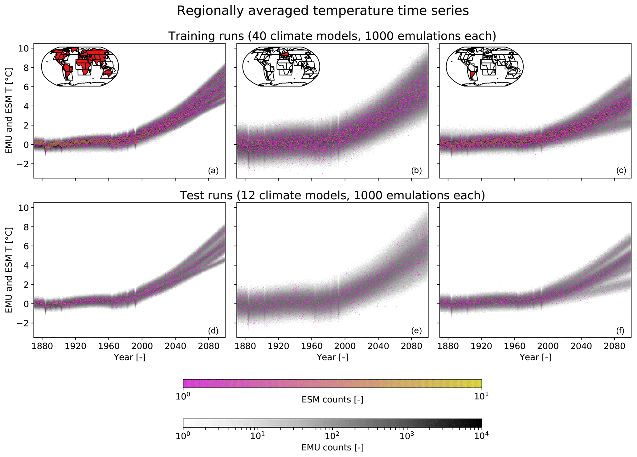
Figure 8 Regionally averaged time series as 2-D histograms for 40 CMIP5 model training runs and 1000 emulations per model (a–c) as well as for 12 CMIP5 models with one test run and 1000 emulations per model (d–f). For the CMIP5 model runs a color map from pink to yellow is employed, and for the emulations a grayscale is used. The regions are global land (a, d), CEU (b, e), and SSA (c, f).

6.3 Quantitative verification

6.3.1 Local trend verification

Correlation between the emulated local trends and the true climate model runs is very high in both training and test runs in all CMIP5 models, indicating that the forced trends are successfully extracted from each training run (Fig. 9). For the climate models with test runs, these correlations are nearly identical for each individual test and the training runs. The smallest correlation coefficient is 0.90, and the highest one is 0.97.

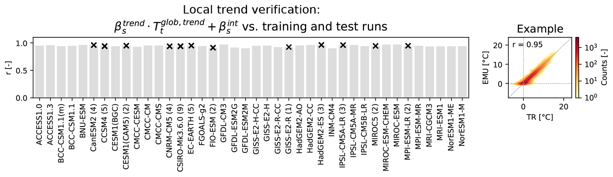
Figure 9 Local trend verification for the CMIP5 models by means of Pearson correlation between the emulated local trends and the training runs (gray bars). The example shows the associated 2-D histogram for CESM1(CAM5). For the CMIP5 models with test runs, the correlation between the emulated local trends and each individual test run is indicated by a black cross. Since these correlations are nearly identical for each test run of a specific climate model, the individual black crosses cannot be visually distinguished from one another. For all climate models with test runs, the number of available test runs is given in brackets after the model name.

6.3.2 Local variability verification

To evaluate the local variability at the grid-point level, lag-1 temporal autocorrelations and standard deviations are considered (Fig. 10). The lag-1 temporal autocorrelation is a rather noisy parameter to estimate, and the median correlations between emulations and the training run lie between 0.67 and 0.92. Generally, the correlation of the lag-1 autocorrelations between test and training runs is smaller than the one between emulations and training runs, implying a tendency to overfit this parameter. The correlation between the standard deviations of the emulations and the training run is never below 0.98. The correlation between test and training runs is almost identical to the one between emulations and training runs. Thus, at the grid-point level the emulations reliably reproduce the stochastic variability of climate model runs.

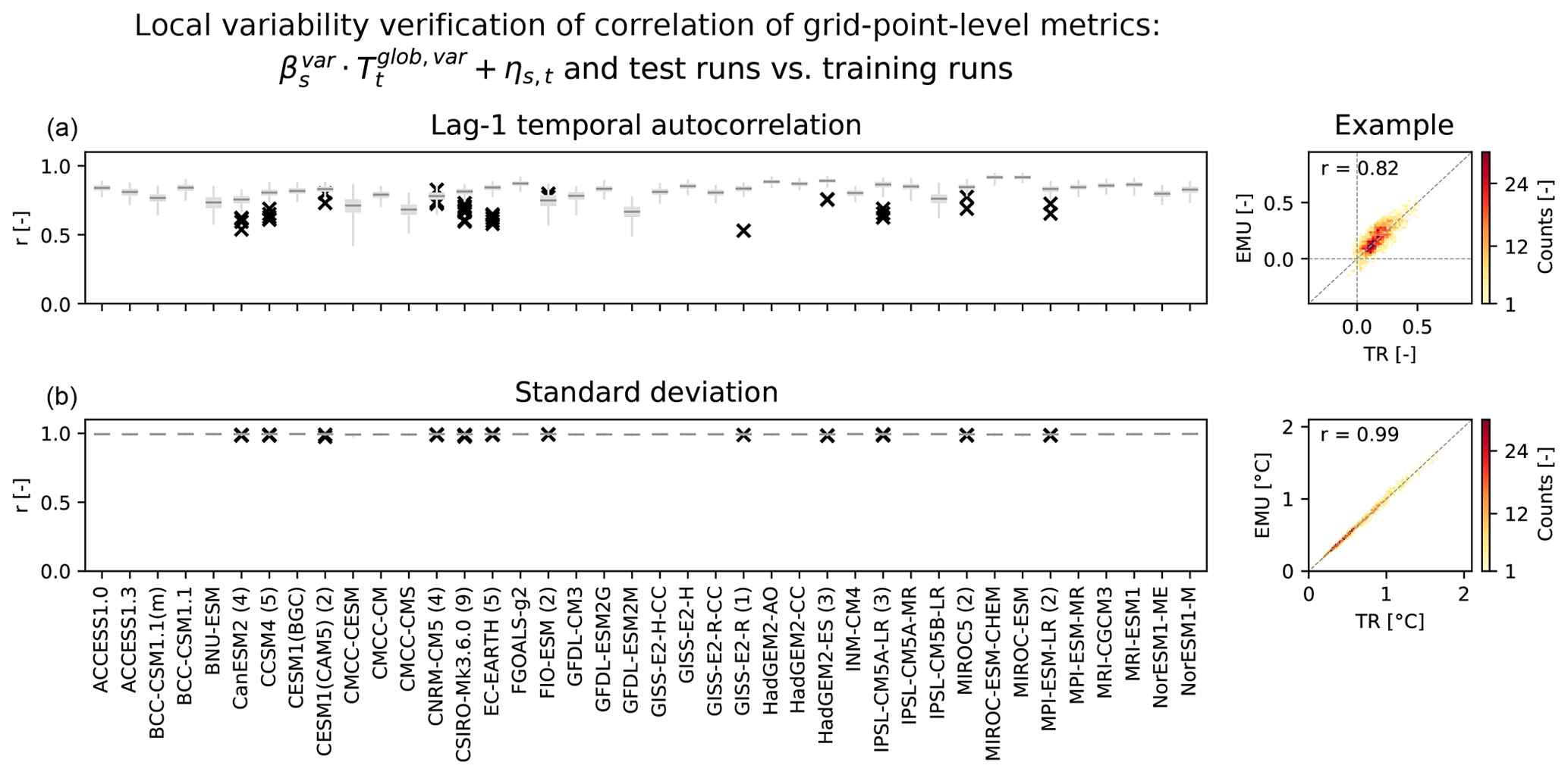
Figure 10 Local variability verification for the CMIP5 models (columns) by means of the Pearson correlation of grid-point-level lag-1 temporal autocorrelations (a) and standard deviations (b) between the 1000 individual emulations and the training runs (box plots). The examples show the associated 2-D histograms for a single emulation and the training run of CESM1(CAM5). For the CMIP5 models with test runs, the correlation between the quantity in the training run and in each individual test run is indicated by a black cross. For all climate models with test runs available, the number of test runs is given in brackets after the model name.

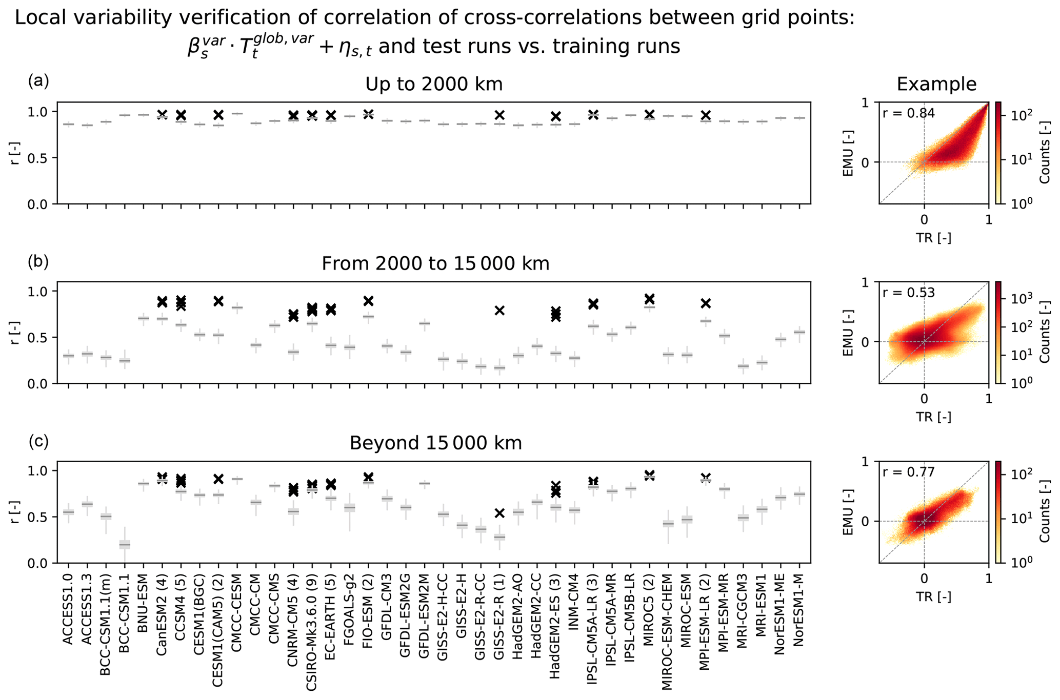
Figure 11 Local variability verification for the CMIP5 models (columns) by means of the Pearson correlation of cross-correlations between grid points in three geographical bands (rows) between the 1000 individual emulations and the training runs (box plots). The geographical bands cover distances below 2000 km (a), between 2000 and 15 000 km (b), and beyond 15 000 km (c). The examples show the associated 2-D histograms for a single emulation and the training run of CESM1(CAM5). For the CMIP5 models with test runs, the correlation between the quantity in the training run and in each individual test run is indicated by a black cross. For all climate models with test runs available, the number of test runs is given in brackets after the model name.

To evaluate the spatial cross-correlations between grid points, three geographical bands are considered (Fig. 11). At all spatial scales, cross-correlations between test and training runs are higher than correlations between emulations and training runs. This is a direct consequence of the regularization, which dampens covariances between grid points as a function of distance and is thus inherent to the emulator's design. In a radius of up to 2000 km, the emulators perform best and covariations between grid points are generally well reproduced. The medians of the correlations between the emulations and the training runs span from 0.85 to 0.98. Plotting an individual example emulation against its associated training run clearly shows the dampening of the cross-correlations in the regularized emulations. Emulations of climate models with larger localization radii (Fig. 7) have by design a larger correlation with their respective training runs (Fig. 11). In a radius between 2000 and 15 000 km, the emulators perform the least well because cross-correlations for this radius are strongly dampened in the emulations, with the medians of the correlations between emulations and training runs ranging from 0.17 to 0.82. For long-range distances beyond 15 000 km, medians lie between 0.20 and 0.93. For all distances beyond 2000 km, there are large inter-model differences in the ability of the emulators to reproduce cross-correlations between grid points. Also, correlations between the spatial cross-correlations of test and training runs are generally lower and exhibit more inter-model differences at distances beyond 2000 km, highlighting that it is more difficult to estimate far-reaching spatial cross-correlation based on single ESM runs. Generally, the emulations perform better and are more comparable to test runs at distances beyond 15 000 km than between 2000 and 15 000 km, which is likely due to that fact that the global correlation pattern induced by the global mean temperature variability serves as a more important driver for the longest-range correlations.

6.3.3 Regional-scale ensemble reliability verification

When considering full emulations, i.e., the local trends plus the local variability, the median is successfully emulated but the emulations are a bit underdispersive compared to the training run for the vast majority of CMIP5 models and SREX regions (Fig 12). The emulations tend to be more reliable for climate models with larger localization radii (Fig. 7). In North Asia (NAS), the underdispersion is strongest for most models (Fig. 12). The only region where the emulations are fully reliable is global land. The underdispersion on the SREX regional scales is related to the regularization, which dampens covariances between grid points as a function of distance between them and is thus inherent to the emulator's design. The results are qualitatively similar for the test runs but, as expected, the deviations from the emulated quantiles tend to be larger in magnitude than for the training runs. For most climate models, the strongest deviations in the median of the test runs are observed in global land, Canada–Greenland–Iceland (CGI), and South Australia–New Zealand (SAU). Out of all climate models, the least optimal fit is obtained for MIROC5, with the emulated median being systematically warmer than the training and especially the test run medians in many regions.

Figure 12 Deviation of climate model runs from the emulated 5 % (a, d), 50 % (b, e), and 95 % (c, f) quantile for CMIP5 models (rows) and regions (columns). The emulated quantile is computed based on 1000 emulations per climate model. The deviation of the climate model run from the emulated quantile is given in color. Red means that the emulated quantile is warmer than the quantile of the climate model run, and blue means that it is colder. The gray numbers indicate how many climate model run deviations lie outside the 95 % interval spanned by the deviations of single emulations from the emulated quantiles. If the climate model run lies outside this interval, it is no longer considered indistinguishable from the emulations. The deviation from the training run is shown in panels (a)–(c), and the average deviation across all available test runs is shown in panels (d)–(f). The number of test runs averaged across is indicated in brackets behind the model names.

7 Discussion

7.1 Emulator design choices and their implications

7.1.1 Modular framework

A modular framework is chosen for the climate model emulation because of its manifold advantages. First, the calibrated parameters of each emulator module can be used for climate model intercomparison over a wide range of scales since they can be readily visualized and easily interpreted (Sects. 5.1 and 6.1). Second, the modular framework renders it straightforward to substitute each emulator module with approaches other than the ones chosen here. For example, alternative approaches for the global mean temperature trend (e.g., Meinshausen et al., 2011), for the local response module (e.g., Tebaldi and Arblaster, 2014; Alexeeff et al., 2018), or for the local residual temperature variability (e.g., Link et al., 2019) could be employed. Third, if the modeling task were to change, additional predictors could easily be integrated. For example, precipitation emulation would likely require human-induced aerosol emissions as an additional predictor in the local response module (Frieler et al., 2012).

7.1.2 Emulating temperature trends

In this study, an estimate of $T_t^{\mathrm{glob},\mathrm{trend}}$ is retrieved with a simple statistical model from the training run (Sect. 4.1.2). However, it could alternatively be considered to obtain $T_t^{\mathrm{glob},\mathrm{trend}}$ from a simple energy balance model (Meinshausen et al., 2011). This would open avenues towards emulating initial-condition ensembles across different $T_t^{\mathrm{glob},\mathrm{trend}}$ trajectories and thus different emission scenario pathways.

To translate $T_t^{\mathrm{glob},\mathrm{trend}}$ into a local temperature in the local response module, a linear approach is chosen (Sect. 4.1.3). The thereby obtained regression coefficients ${\mathit{\beta }}_s^{\mathrm{trend}}$ represent well-known climate phenomena. The enhanced warming over land compared to the global mean (Sutton et al., 2007; Hartmann et al., 2013) at many grid points is captured by ${\mathit{\beta }}_s^{\mathrm{trend}}>\mathrm{1}$ (Figs. 3 and 7). The Arctic amplification (Serreze and Barry, 2011) manifests itself in the large ${\mathit{\beta }}_s^{\mathrm{trend}}$ values in northern high latitudes (Fig. 3). The overall good performance in capturing local trends is in line with the pronounced linear scaling of regional land temperatures with global mean temperature (Seneviratne et al., 2016; Wartenburger et al., 2017) and the widely used linear pattern scaling approaches (Mitchell, 2003; Tebaldi and Arblaster, 2014; Lynch et al., 2017; Osborn et al., 2018).

7.1.3 Emulating temperature variability

Spatially coherent local variability is introduced in two emulator modules, namely in the local response module as the local response to $T_t^{\mathrm{glob},\mathrm{var}}$ (Sect. 4.1.3) and in the local residual variability module (Sect. 4.1.4). The local variability is an essential ingredient in mimicking initial-condition ensembles as visualized by comparing the regionally averaged time series of our emulations with simple pattern scaling results which contain no local variability module (Fig. S11). In this study, and all other studies cited in the following paragraphs, the local temperature variability is assumed to be stationary in time, which is not fulfilled everywhere in the business-as-usual greenhouse gas emission scenario (see Sect. 2.3 and Olonscheck and Notz, 2017).

$T_t^{\mathrm{glob},\mathrm{var}}$ can be regarded as the globally aggregated signal of all physical modes of variability (Sect. 4.1.2), with the calibrated emulators accounting for memory of up to 3 years (Fig. 7). While the linear translation of $T_t^{\mathrm{glob},\mathrm{var}}$ to a grid-point-level temperature response is purely statistical in nature, physically meaningful patterns nevertheless emerge in the ${\mathit{\beta }}_s^{\mathrm{var}}$ patterns. For example, for many climate models, ${\mathit{\beta }}_s^{\mathrm{var}}$ tends to resemble an El Niño–Southern Oscillation pattern (Trenberth, 1997) with the Amazon, Australia, and Alaska covarying, while the southeastern USA exhibits the opposite temperature sign (Figs. 3 and S2–10). Qualitatively similar results could alternatively be obtained by stochastically generating time series of major physical modes of variability and translating those to the grid-point level (McKinnon and Deser, 2018).

Local residual variability is modeled as an AR process with spatially correlated innovations (Sect. 4.1.4). While several other authors have employed AR models with spatially correlated innovations (Castruccio and Stein, 2013; Castruccio and Genton, 2016; Bao et al., 2016), they all chose a parametric approach to model the covariance between grid points. However, in this study, a nonparametric approach is employed, which retains regional-scale anisotropy in the underlying data.

7.2 The pros and cons of training on single climate model runs

We demonstrated that, for yearly temperature at grid-point to regional scales, training on a single run per climate model is sufficient to learn the key properties of the climate system of this climate model. Early results furthermore indicated that larger single-model initial-condition ensembles, in that case a 21-member CESM ensemble, can also be successfully emulated when training on a single ESM run (Beusch et al., 2018). Since a single run was submitted for the majority of climate models participating in CMIP5 for the emission pathway considered here, requiring only one run to train the emulator provides the opportunity to emulate a much larger multi-model ensemble and thus to have the resulting superensemble account for more inter-model uncertainty. Nevertheless, it is not possible to reproduce the characteristics of a true ESM at all spatial and temporal scales when training on a single run. To obtain the best possible emulations to be used, e.g., for uncertainty propagation in climate impact or integrated assessment models, it is thus advisable to employ all available runs for training instead of just a single one for each climate model. When training on multiple runs, the parameters of the emulator can be estimated more robustly, which, among other things, results in a larger localization radius and thus the ability to reproduce farther-reaching spatial cross-correlations between grid points.

7.3 Large single-model initial-condition vs. large multi-model ensembles

Our results highlight fundamental differences between large single-model initial-condition ensembles (Deser et al., 2012; Fischer et al., 2013; Kay et al., 2015; Leduc et al., 2019; Maher et al., 2019) and large multi-model ensembles (Meehl et al., 2007; Taylor et al., 2012; Eyring et al., 2016). While multi-model ensembles are imperfect, with several ESMs exhibiting dependencies (Knutti, 2010; Bishop and Abramowitz, 2013; Sanderson et al., 2015; Abramowitz et al., 2019), multi-model uncertainty nevertheless clearly exceeds single-model initial-condition uncertainty at the yearly scale for temperature (Sect. 5.3). ESMs contained within CMIP5 differ substantially across a broad range of scales and thus sample different phase spaces in projections, which renders it necessary to train an emulator on each climate model to approximate the CMIP5 ensemble. A single-model initial-condition ensemble, on the other hand, can be successfully mimicked on grid-point to regional scales by training on a single ESM run (Sects. 5 and 6). While this lies beyond the scope of this study, the developed emulator could additionally serve as a novel tool to address the challenge of inter-model dependencies. Differences between climate models could be quantified in terms of their emulator parameters, and subsequently a subset of models with sufficiently divergent parameters could be selected to base projections on. Additionally, observations could be used to constrain the emulated ensemble by providing validation measures for the emulator parameters.

8 Conclusions and outlook

We introduce a modular framework for climate model emulation of yearly land temperatures and present a specific, computationally cheap implementation called MESMER, which can create plausible temperature field time series within seconds based on a single climate model training run. Our emulator consists of (i) a global mean temperature module, (ii) a local temperature response module, and (iii) a local residual temperature variability module. The global mean temperature module contains a global mean temperature trend, which is shared by all emulations, and a global mean temperature variability term, which is modeled as an AR process and varies between individual emulations. The local response module is linear in nature and consists of a separate response to the global mean temperature trend and the global mean temperature variability. The local residual variability module generates spatiotemporally correlated fields by means of locally fit AR(1) processes with spatially correlated innovations.

Since emulators approximate complex ESMs in a simplified manner, they are not able to accurately reproduce all spatiotemporal ESM characteristics. The emulator presented here, e.g., dampens covariations between grid points as a function of distance in the local residual variability module due to regularization. Thus, our emulator reliably reproduces climate model variability at the grid-point level, but the emulations are increasingly underdispersive for larger regional averages and intermediate-range spatial teleconnections cannot be accounted for. This caveat could be addressed by further improving the local residual variability module implementation with a focus on such teleconnections. Alternatively, training on several ESM runs would increase the robustness of the estimated parameters and make it possible to reproduce farther-reaching teleconnections within the current emulator setup. Nevertheless, calibrating our emulator on a single training run is sufficient to generate emulations which are visually indistinguishable from true ESM runs.

Inherent inter-ESM differences in warming trends and spatiotemporal variability make it necessary to calibrate a separate emulator for each of the 40 considered CMIP5 models. The resulting emulations successfully approximate the training run for each climate model on grid-point to regional scales. For CMIP5 models with more than one initial-condition ensemble member, it was furthermore demonstrated that the ensemble of emulations is generally able to mimic true climate model initial-condition ensembles at these scales. Hence, we argue that to sample climate signal uncertainty for yearly temperature at grid-point to regional scales, it is more advantageous to invest computational resources into generating multi-model ensembles rather than large single-model ensembles, since the latter can be readily approximated by our emulator.

Superensembles such as the one generated in this study, which contains 1000 emulations per climate model, are expected to be particularly helpful in regions with large interannual variability. There, the very sparse sampling of the temperature phase space by the CMIP5 ensemble may result in biased conclusions when solely employing the CMIP5 ensemble as an input to impact or integrated assessment models which estimate the effect of climate signal uncertainty on their quantity of interest.

The emulator is designed to be flexible enough to emulate whatever climate model run it is provided with. Hence, it is not part of the emulator's tasks to judge the realism of individual climate models. Instead, the choice of considered ESMs will depend on the scope of different applications. For example, results from emergent constraints analyses (e.g., Hall and Qu, 2006; Eyring et al., 2019) could be combined with the implementation of an emulator to derive a superensemble based on an observationally constrained set of ESMs. On the other hand, the emulator parameters could themselves be used as potential constraints that can also be derived from observations. Additionally, the emulator parameters can be regarded as an ESM-specific “model ID”, which provides an interesting avenue for climate model intercomparison across a wide range of scales. Inter-model differences can be readily visualized for every emulator module, resulting in comprehensible scale-dependent insights into the underlying properties of each climate model. Future work could focus on extending the emulator to simultaneously generate multivariate output. Furthermore, it would be interesting to investigate how transferable an emulator trained on a specific greenhouse gas emission scenario is to other emission pathways and which modules would need to be modified to account for inter-scenario differences.

In conclusion, in this study we have presented a novel ESM emulator called MESMER that can be trained to represent separate ESMs based on single realizations of the respective ESMs and which has been shown to be able to emulate and expand multi-model ensembles such as CMIP5. We expect that the developed emulator can serve as a training ground for investigating the phase space of multi-model ensembles in new applications, e.g., related to the derivation of emissions scenarios or the assessment of impacts under different emissions pathways.

Appendix A

Table A1 List of the 40 employed CMIP5 models, the modeling groups providing them, and the number of initial-condition ensemble members used.