Predicting near-term variability in ocean carbon uptake

Interannual variations in air–sea fluxes of carbon dioxide (CO₂) impact the global carbon cycle and climate system, and previous studies suggest that these variations may be predictable in the near term (from a year to a decade in advance). Here, we quantify and understand the sources of near-term predictability and predictive skill in air–sea CO₂ flux on global and regional scales by analyzing output from a novel set of retrospective decadal forecasts of an Earth system model. These forecasts exhibit the potential to predict year-to-year variations in the globally integrated air–sea CO₂ flux several years in advance, as indicated by the high correlation of the forecasts with a model reconstruction of past CO₂ flux evolution. This potential predictability exceeds that obtained solely from foreknowledge of variations in external forcing or a simple persistence forecast, with the longest-lasting forecast enhancement in the subantarctic Southern Ocean and the northern North Atlantic. Potential predictability in CO₂ flux variations is largely driven by predictability in the surface ocean partial pressure of CO₂, which itself is a function of predictability in surface ocean dissolved inorganic carbon and alkalinity. The potential predictability, however, is not realized as predictive skill, as indicated by the moderate to low correlation of the forecasts with an observationally based CO₂ flux product. Nevertheless, our results suggest that year-to-year variations in ocean carbon uptake have the potential to be predicted well in advance and establish a precedent for forecasting air–sea CO₂ flux in the near future.

1 Introduction

Observations collected over the past few decades indicate that the ocean has absorbed 160 Pg of excess carbon from the atmosphere since the beginning of the industrial revolution (Le Quéré et al., 2018); projections from climate models suggest that ∼540 Pg of excess carbon will reside in the ocean by the end of the century (Ciais and Sabine, 2013). Accurate projections of past and future air–sea CO₂ flux are important for quantifying and understanding the changing global carbon cycle and for estimating future global climate change (Le Quéré et al., 2018).

Superimposed on the background of long-term changes in ocean carbon uptake is substantial variability on global and regional scales (Landschützer et al., 2016; McKinley et al., 2017). The recent literature highlights ocean carbon uptake variability that manifests on timescales of years to decades. Interannual variability in globally integrated air–sea CO₂ flux has been estimated to have a standard deviation of 0.31 and 0.2 Pg C yr⁻¹ from observationally based products (Rödenbeck et al., 2015) and ocean biogeochemical models (Wanninkhof et al., 2013), respectively, which is of the order of 10 % of the global mean CO₂ flux (2.3 Pg C yr⁻¹). A global extrapolation of sparse pCO₂ observations suggests that there is large variability on decadal timescales (Landschützer et al., 2016). On regional scales, Southern Ocean studies have highlighted recent air–sea CO₂ flux variability on interannual (Hauck et al., 2013; Lenton and Matear, 2007; Lenton et al., 2013; Lovenduski et al., 2007, 2013, 2015a; Verdy et al., 2007; Wang and Moore, 2012; Wetzel et al., 2005) and decadal (Fay et al., 2014; Landschützer et al., 2015; Munro et al., 2015) timescales. In the North Atlantic, high air–sea CO₂ flux variability has been linked to the North Atlantic Oscillation (Thomas et al., 2008; Ullman et al., 2009) and the Atlantic Multidecadal Oscillation (Breeden and McKinley, 2016; Metzl et al., 2010), whose spectra peak at interannual and multi-decadal timescales.

Near-term predictions of the climate system (so-called “decadal predictions”) are forecasts of climate variability and change on annual, multi-annual, and decadal timescales from global climate models (Meehl et al., 2014). These forecasts are sensitive to both initial conditions (e.g., the atmospheric temperature used to initialize the forecasts) and external forcing (Kirtman et al., 2013). Recent publications highlight near-term predictability and predictive skill in regional surface air temperature, precipitation, Arctic sea ice concentration, oceanic heat content, and the large-scale Atlantic Ocean circulation (Boer et al., 2016; Keenlyside et al., 2008; Meehl et al., 2009, 2014; Robson et al., 2012; Smith et al., 2007; Yeager and Robson, 2017; Yeager et al., 2012, 2015). As prior literature has established a strong link between air–sea CO₂ flux and variability in the physical climate system on these timescales (McKinley et al., 2017; Resplandy et al., 2015), it follows that air–sea CO₂ flux may be predictable in the near term.

Here, we analyze a novel set of decadal prediction simulations from an Earth system model (ESM) to investigate near-term predictions of global and regional ocean carbon uptake. On annual to decadal timescales, ESM predictions of the past (so-called “retrospective forecasts”) are used to assess both predictability and predictive skill in air–sea CO₂ flux. Predictability is the potential to predict the system based on forecast verification against a model reconstruction. Predictive skill is based on forecast verification against observations. We further assess the role of external forcing in the predictability of CO₂ flux by analyzing a set of uninitialized forecasts run under identical external forcing. By analyzing forecasts of the past, our study establishes a precedent for making skillful predictions of ocean carbon uptake in the near future.

2 Community Earth System Model Decadal Prediction System

Our primary numerical tool is the Community Earth System Model Decadal Prediction Large Ensemble (Yeager et al., 2018). In this section, we describe the model and provide details about forecast initialization, ensemble generation, and drift correction. Importantly, we note that this is the first CESM decadal prediction system to include a representation of ocean biogeochemistry. CESM-DPLE uses the same code base as the CESM Large Ensemble (Kay et al., 2015).

The CESM is a state-of-the-art coupled climate model consisting of atmosphere, ocean, land, and sea ice component models (Danabasoglu et al., 2012; Hunke and Lipscomb, 2008; Hurrell et al., 2013; Lawrence et al., 2012). The ocean physical model (Danabasoglu et al., 2012) has nominal 1^∘ horizontal resolution and 60 vertical levels. The biogeochemical ocean model represents the lower trophic levels of the marine ecosystem (Moore et al., 2004, 2013), full carbonate system thermodynamics (Long et al., 2013), air–sea CO₂ fluxes, and a dynamic iron cycle (Doney et al., 2006; Moore and Braucher, 2008).

CESM-DPLE consists of a set of initialized, fully coupled integrations of CESM that adhere to the protocols for Component A of the Decadal Climate Prediction Project (Boer et al., 2016). We use the CESM-DPLE system (Yeager et al., 2018) that builds on previous CESM decadal prediction efforts (Yeager et al., 2012, 2015) with some modifications (including the addition of ocean biogeochemistry, as noted above). CESM-DPLE initiates 40 decade-long “forecasts” of the Earth system each year from 1954–2015; the start date for each forecast is 1 November, in accordance with the DCPP protocols. Each of the model integrations is subject to a common set of historical external forcings (e.g., greenhouse gas concentrations).

The ocean physical and biogeochemical initial conditions for the DP experiments are generated from a forced ocean–sea ice simulation of the CESM. That is, a simulation of the ocean and ice components of the CESM that has been forced with fluxes computed from the observed atmospheric state over 1948–2015. This simulation is therefore meant to reconstruct the historical evolution of the ocean physical and biogeochemical state over the 1948–2015 period (Fig. 1). Hereafter, we refer to this simulation as the “reconstruction”. Initial conditions from the atmosphere and land components of the DP experiments are obtained from a 20th century simulation of the CESM Large Ensemble (Kay et al., 2015).

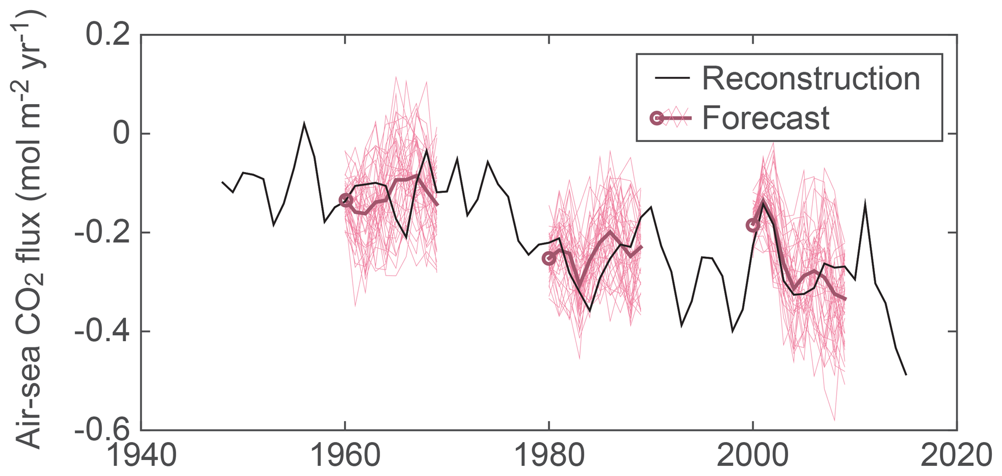
Figure 1 Annual mean air–sea CO₂ flux (mol m⁻² yr⁻¹) in the South Pacific subtropical permanently stratified biome for the (black) model reconstruction and (pink) CESM-DPLE decadal forecasts initiated in 1960, 1980, and 2000 (other forecasts omitted for visual clarity). The thick magenta line represents the ensemble mean forecast; open circles show the ensemble mean in forecast year 1. Positive fluxes denote ocean outgassing. Forecasts have been drift-corrected and adjusted to match the reconstruction climatological mean for ease of visual comparison.

Ocean biogeochemistry in the version of the CESM used for CESM-DPLE has been extensively validated in the literature (Freeman et al., 2018; Krumhardt et al., 2017; Long et al., 2016; Lovenduski et al., 2016; McKinley et al., 2016). In particular, the simulated mean, variability, and trends in surface ocean pCO₂ and air–sea CO₂ flux from CESM over 1982–2011 compare favorably to estimates from observations for the global average and over most ocean biogeochemical biomes (Lovenduski et al., 2016; McKinley et al., 2016). In Fig. 2, we illustrate the comparison between observationally based estimates of CO₂ flux (from the Landschützer et al., 2016, pCO₂ product) and estimates produced by the reconstruction and coupled CESM-LE over 1982–2015. The model reconstruction does a reasonable job (r=0.79) of representing observed spatial patterns (in both magnitude and direction) of the flux across most oceanic regions. The globally integrated air–sea CO₂ fluxes over 1982–2015 from the observational product and model reconstruction are 1.41 and 1.80 Pg C yr⁻¹, respectively (directed into the ocean).

CESM-DPLE initializes an ensemble of 40 simulations each year using round-off-level (order 10⁻¹⁴) perturbations in the initial air temperature field (Fig. 1). Previous work indicates that this small perturbation in the initial conditions generates a wide divergence in global mean surface temperatures across the ensemble members within about 30 days (Vineel Yettella, personal communication, 2018), and the average divergence in globally integrated, annual mean forecast CO₂ flux across the ensemble members (0.53 Pg C yr⁻¹) is an order of magnitude greater than that generated by the preindustrial control simulation of CESM (Lovenduski et al., 2015b). Each ensemble member is subject to identical external forcing. The number of ensemble members in each forecast ensures statistically robust drift estimates (Boer et al., 2013; Kirtman et al., 2013; Yeager et al., 2018).

Following initialization, the coupled model drifts toward its preferred state over the decadal forecast. This is a common problem for full-field initialization decadal prediction experiments (Meehl et al., 2014) and requires a drift correction to be applied to the model forecasts before predictability and predictive skill may be analyzed. We correct the drift by transforming to anomalies from a drifting climatology, as in Yeager et al. (2012, 2018). For a given forecast, X(L, M, S), where L is the forecast length, M is the ensemble member, and S is the start year of the forecast; the drift-corrected forecast anomaly, X^′(L, M, S), is defined as

$$\begin{array}{}\text{(1)}& {\displaystyle }{\displaystyle }{X}^{\prime }(L,M,S)=X(L,M,S)-{\stackrel{\mathrm{‾}}{X(L,M,S)}}^{M,S},\end{array}$$

where ${\stackrel{\mathrm{‾}}{X(L,M,S)}}^{M,S}$ is the average rate of drift over all forecasts. Note that this method does not assume that the drift is linear and disregards potential dependence of the drift on the external forcing.

Predictive skill in CESM-DPLE may be enabled by external forcing (e.g., the time evolution of atmospheric greenhouse gases) as well as by initialization. To assess the role of initialization in predictability, we compare CESM-DPLE air–sea CO₂ flux (generated with the initialization procedure described above) with air–sea CO₂ flux from the CESM-LE (Lovenduski et al., 2016; McKinley et al., 2016) over the same historical period. The CESM-LE is a 32-member ensemble of the CESM with fully resolved ocean biogeochemistry that evolves the Earth system from 1920 to 2100 under historical and RCP8.5 forcing (Kay et al., 2015). As such, CESM-LE represents the uninitialized counterpart to the CESM-DPLE system; output from CESM-LE can tell us how the modeled air–sea CO₂ flux would evolve over a given decade in the absence of initialization, but under the same external forcing.

3 Results

3.1 Predictability

Predictability is a property of a system that characterizes the potential for its future evolution to be predicted; this concept is distinct from that of model skill. We quantify predictability by evaluating the ability of the CESM-DPLE initialized forecasts to predict variations in air–sea CO₂ flux from the reconstruction. For a given forecast anomaly, X^′(L, M, S), predictability is defined as the correlation coefficient of X^′(L, M, S) with the corresponding anomaly in the reconstruction; the reconstruction anomaly is obtained by subtracting the climatological mean value over 1955–2015.

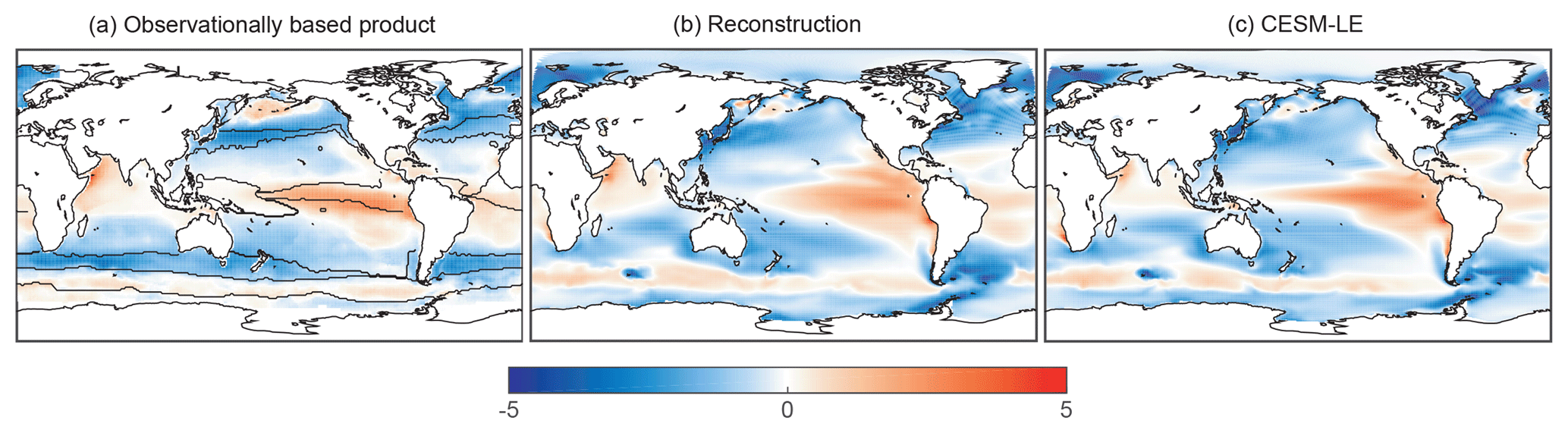
Figure 2 Annual mean air–sea CO₂ flux (mol m⁻² yr⁻¹) over the period 1982–2015 as estimated by (a) the Landschützer et al. (2016) observationally based product, (b) the model reconstruction, and (c) the CESM-LE. Positive fluxes denote ocean outgassing, and black contours in (a) show biome boundaries.

The globally integrated air–sea CO₂ flux anomaly from the initialized CESM-DPLE in forecast year 1 exhibits high correlation with the CO₂ flux anomaly from the reconstruction (Fig. 3a; r=0.98). This correlation remains high and statistically significant (at the 95 % level using a two-sided Student's t test while accounting for autocorrelation in the sample size) for 10 forecast lead years (Fig. 3c), suggesting high, long-lasting predictability in the globally integrated air–sea CO₂ flux.

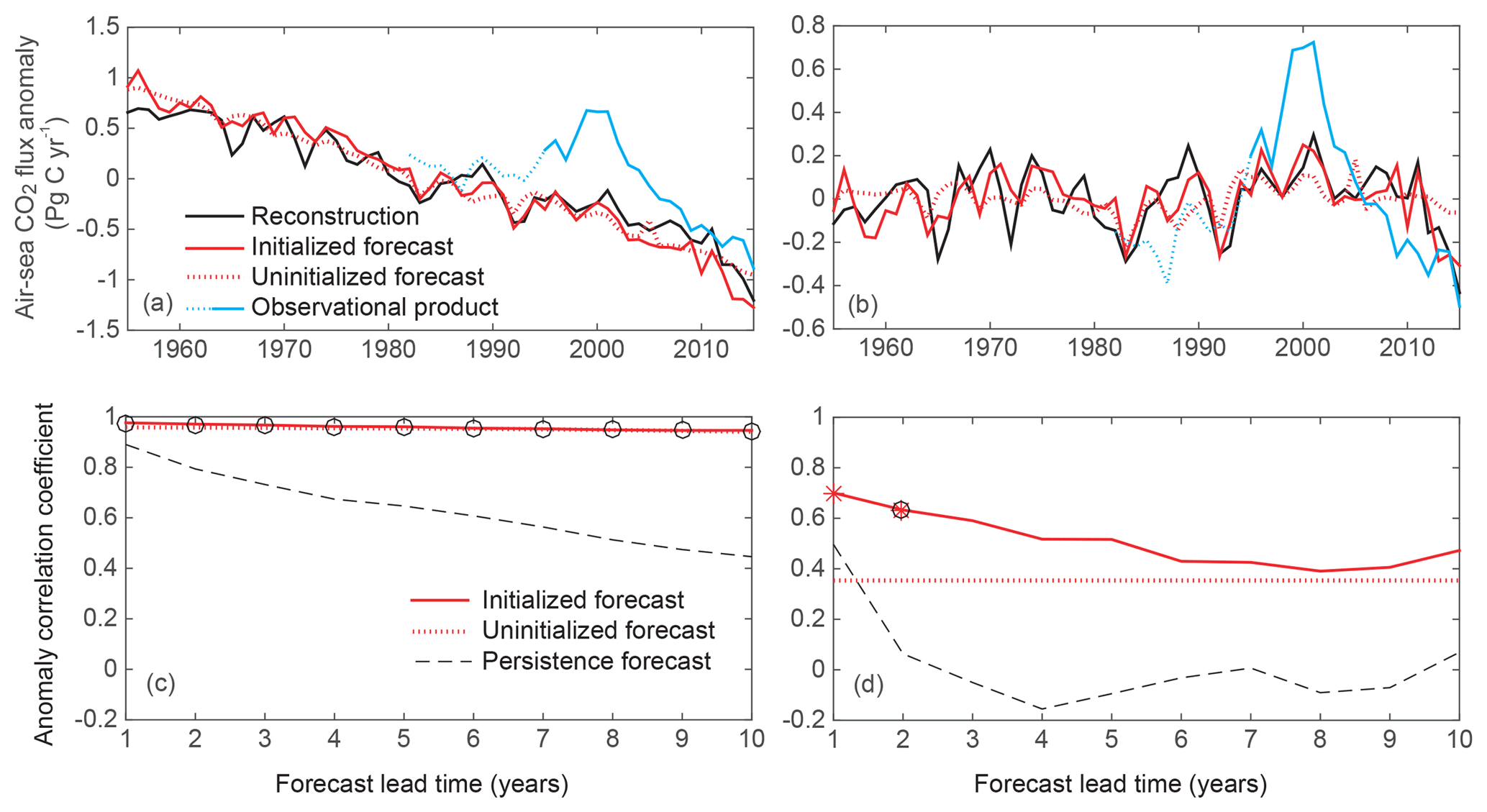
Figure 3 (a) Temporal evolution of the globally integrated air–sea CO₂ flux anomaly, as estimated by the (black) reconstruction, (red) CESM-DPLE initialized forecast, (red dotted) CESM-LE uninitialized forecast, and (blue) Landschützer et al. (2016) observationally based product. The CESM-DPLE time series is the drift-corrected, ensemble mean forecast anomalies over lead year 1; the reconstruction, uninitialized forecast, and observational product have been transformed to anomalies by subtracting their respective climatological means. Observations prior to 1995 are dotted due to lower observation density. Positive anomalies indicate anomalous ocean outgassing. (b) Same as (a), but with long-term linear trends removed from each time series. (c) Predictability of globally integrated CO₂ flux as a function of lead time, as indicated by the correlation coefficient of CO₂ flux anomalies from the (red) CESM-DPLE initialized forecast, and the (red dotted) CESM-LE uninitialized forecast with the reconstruction. The black dashed line indicates the correlation coefficient of the persistence forecast as a function of lead time. Red asterisks (black circles) on the initialized forecast indicate predictability that is statistically different from the uninitialized (persistence) forecast at the 95 % level using a z test. (d) Same as (c), but with linear trends removed from each time series.

We further investigate whether the predictability in the globally integrated air–sea CO₂ flux is a function of initialization by (1) correlating integrated CO₂ flux anomalies from the ensemble mean of the uninitialized CESM-LE simulation with anomalies from the reconstruction and (2) generating a persistence forecast (autocorrelation as a function of lead time) for the CO₂ flux anomalies from the reconstruction. Figure 3a and c reveal that the initialization of the forecast does not much improve the prediction from the uninitialized forecast. This is because the strong externally forced component of the forecast (e.g., the rising CO₂ concentration in the atmosphere) provides an important source of predictability in both the initialized and uninitialized forecasts. While the persistence forecast also yields high correlation coefficients, both the initialized and uninitialized forecasts beat persistence for all prediction lead times (Fig. 3c).

Figure 3a also reveals interannual variability in the globally integrated air–sea CO₂ flux. While this variability is swamped by the externally forced signal (i.e., the increasing CO₂ uptake due to rising atmospheric CO₂), we are nevertheless interested in the ability of CESM-DPLE to forecast this year-to-year variability. To accomplish this, we remove the linear trend from the forecasts and the reconstruction before computing predictability; this method produces estimates of correlation that are not dominated by the trend induced by external forcing. The globally integrated, detrended air–sea CO₂ flux anomaly from the initialized CESM-DPLE in lead year 1 exhibits high correlation with CO₂ flux from the reconstruction (Fig. 3b; r=0.70), suggesting high predictability of ocean carbon uptake variability on interannual timescales as well. While this predictability drops off with forecast lead time, we nevertheless find high correlations (r>0.5) between the annual mean CO₂ flux forecast anomalies and detrended reconstruction anomalies that extend for 4 years (Fig. 3d).

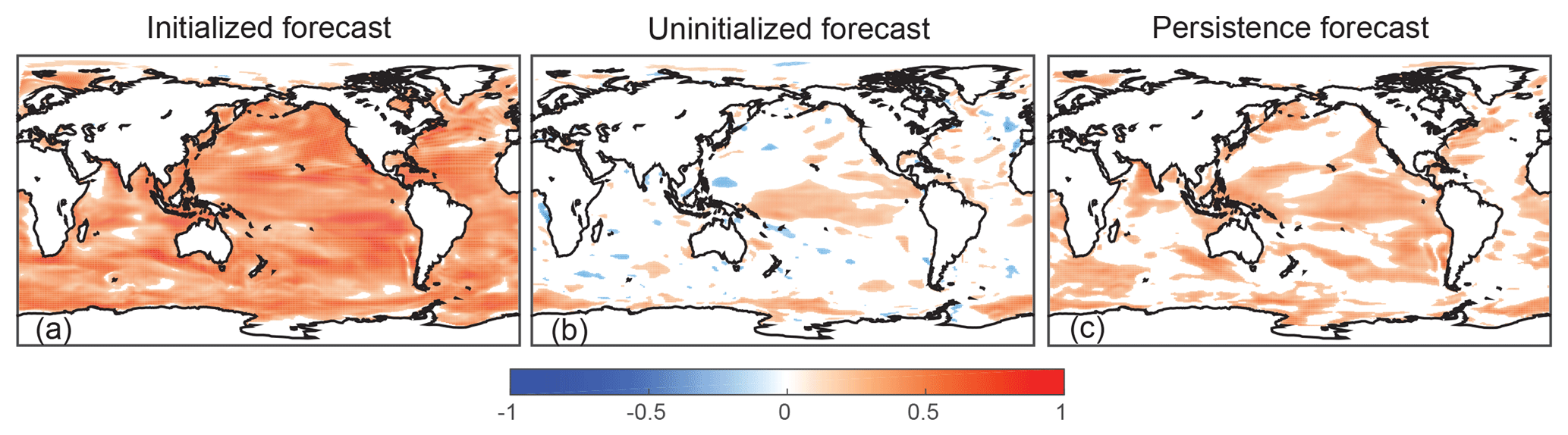
Figure 4 Predictability of air–sea CO₂ flux, as indicated by the correlation coefficient of detrended air–sea CO₂ flux anomalies from the (a) CESM-DPLE initialized forecast lead year 1 with the reconstruction and the (b) CESM-LE uninitialized forecast with the reconstruction. (c) Correlation coefficient of the persistence forecast for lead year 1. Correlation coefficients that are not statistically significant at the 95 % level using a t test are assigned a value of zero.

Interannual variability in global air–sea CO₂ flux may also be affected by interannual variability in external forcing (e.g., volcanoes). As above, we evaluate the role of initialization by calculating uninitialized predictability and estimating persistence. Figure 3 indicates that the initialized forecast exhibits higher predictability than the uninitialized forecast and the persistence forecast for a lead time of 10 years, though this initialized predictability is only statistically separable from the uninitialized and persistence forecasts for lead years 1–2 and 2, respectively; statistical separation was determined via a Fisher's r to z transformation and a comparison of the resulting z test statistic to the value for the 95 % confidence interval (1.96). Thus, the CESM-DPLE initialized forecasts have the potential to predict year-to-year variations of globally integrated air–sea CO₂ flux several years in advance.

The results from our analysis of the globally integrated air–sea CO₂ flux suggest that interannual variations in global ocean carbon uptake may be predictable in advance. They further indicate that initialization of the forecasts enhances the predictability of future interannual variations over and above the predictability from variations in the external forcing, such as those imposed by volcanic eruptions. This is a particularly meaningful result for those forecasting year-to-year changes in the global carbon budget (Le Quéré et al., 2018), especially as these forecasting efforts are blind to the externally forced variability in advance (i.e., the external forcing of the future is unknown). In this way, near-term predictions of air–sea CO₂ flux variations can help to inform future predictions of land–air CO₂ flux and atmospheric CO₂.

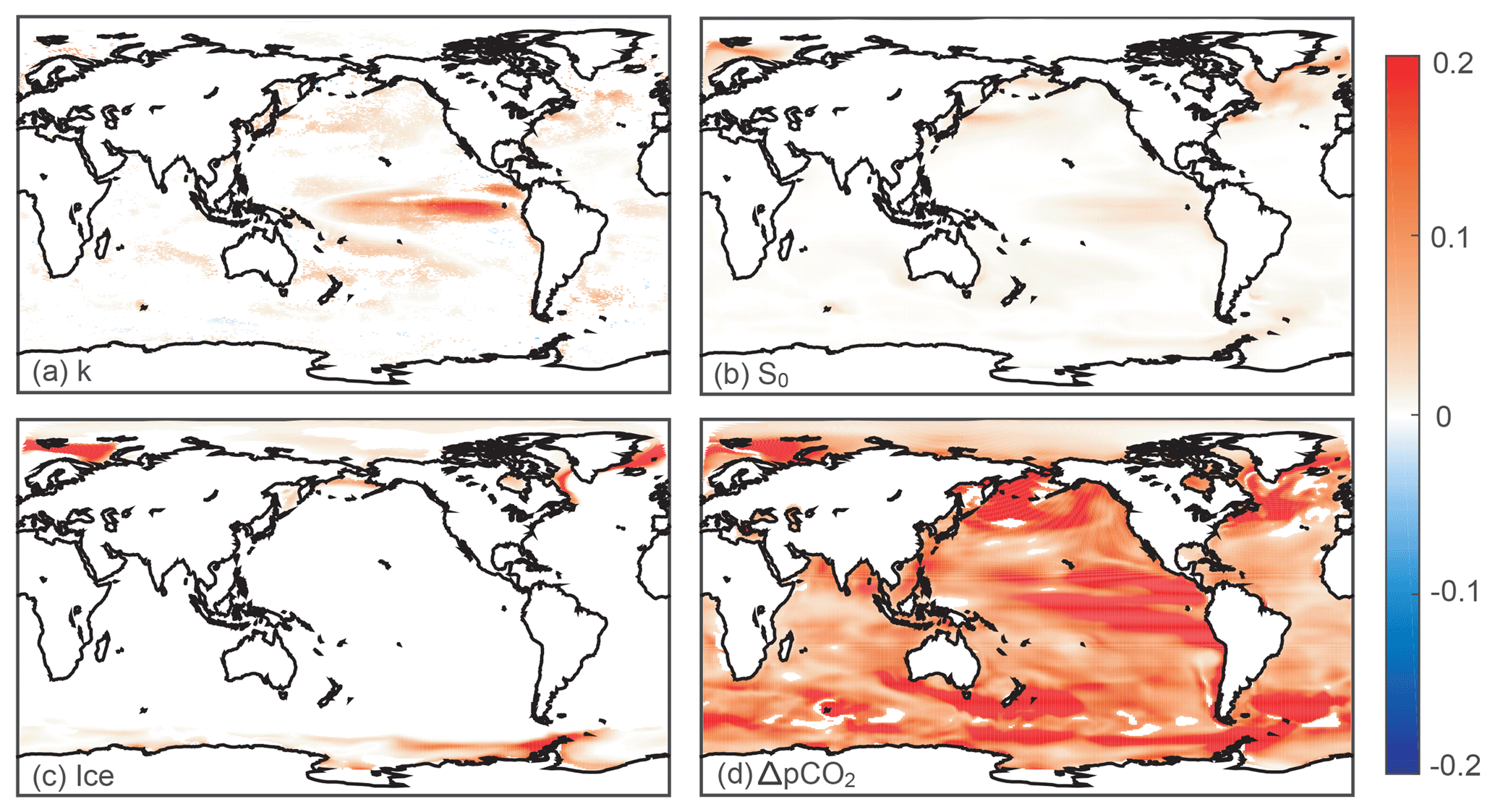
Figure 5 Drivers of predictability in air–sea CO₂ flux during forecast year 1, as indicated by the predictability of the (a) gas exchange coefficient, (b) solubility, (c) sea ice fraction, and (d) ΔpCO₂, scaled to CO₂ flux units (mol m⁻² yr⁻¹). Correlation coefficients that are not statistically significant at the 95 % level using a t test are assigned a value of zero.

Given the high predictability and the important role of initialization in forecasts of interannual air–sea CO₂ fluxes on a global scale, we next investigate the spatial patterns of air–sea CO₂ flux predictability across the global ocean. Here, we use the same statistical techniques as for the global flux, but instead perform an analysis in each model grid cell. On a global scale, the evolution of air–sea CO₂ flux is dominated by the long-term increase in ocean uptake (see, e.g., Fig. 3a), whereas on local and regional scales, the evolution is dominated by interannual variability (Lovenduski et al., 2016). To capture the predictability on interannual timescales, we perform an analysis on linearly detrended forecasts in each model grid cell. Figure 4a illustrates the large predictability of initialized CO₂ flux across much of the global ocean for forecast lead year 1 (additional forecast lead years shown in Fig. S1 in the Supplement). The uninitialized forecast (Fig. 4b) and the persistence forecast (Fig. 4c) indicate lower predictability.

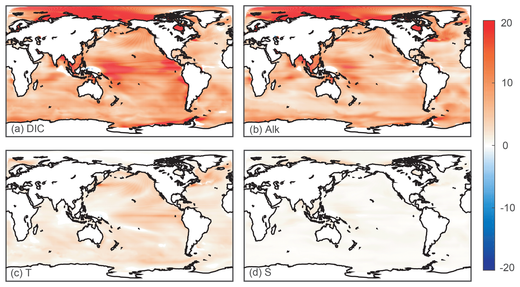
Figure 6 Drivers of predictability in surface ocean pCO₂ during forecast year 1, as indicated by the predictability of surface ocean (a) DIC, (b) Alk, (c) temperature, and (d) salinity, scaled to pCO₂ units (µatm). Correlation coefficients that are not statistically significant at the 95 % level using a t test are assigned a value of zero.

If not external forcing or persistence, what drives the high predictability in air–sea CO₂ flux interannual variability? We decompose the predictability of air–sea CO₂ flux (Φ) over forecast lead year 1 by considering the predictability of its drivers:

$$\begin{array}{}\text{(2)}& {\displaystyle }{\displaystyle }\mathrm{\Phi }=k\cdot S_{\mathrm{0}}\cdot (\mathrm{1}-\mathrm{ice})\cdot \mathrm{\Delta }p{\mathrm{CO}}_{\mathrm{2}},\end{array}$$

where k is the piston velocity (also known as the gas transfer coefficient), S₀ is the solubility of CO₂ in seawater, “ice” is the fraction of the ocean covered by sea ice, and ΔpCO₂ is the difference between the oceanic pCO₂ and the atmospheric pCO₂. As for CO₂ flux, predictability is defined as the anomaly correlation coefficient of each driver variable in forecast year 1 with the corresponding anomaly of that driver variable in the reconstruction, e.g., the correlation of anomalous piston velocities from the forecast with those from the reconstruction. Figure 5 shows the predictability of each of the CO₂ flux driver variables; the anomaly correlation coefficients are scaled to CO₂ flux units (mol m⁻² yr⁻¹) and can be easily compared. The predictability scaling is achieved by multiplying the anomaly correlation coefficient (r) by the sensitivity of CO₂ flux to each driver variable (x) and the standard deviation of the driver variable time series:

$$\begin{array}{}\text{(3)}& {\displaystyle }{\displaystyle }r\cdot {\displaystyle \frac{\partial \mathrm{\Phi }}{\partial x}}\cdot {\mathit{\sigma }}_x,\end{array}$$

where the sensitivities and standard deviations are established from model-estimated, annual mean quantities in each grid cell (Lovenduski et al., 2007, 2013, 2015a) using annual averages from the reconstruction. The CO₂ flux predictability is largely driven by predictability in ΔpCO₂ across the global ocean (Fig. 5). Our results suggest secondary roles for the piston velocity in the equatorial Pacific, solubility in the North Atlantic subpolar gyre, and sea ice fraction in the Arctic–North Atlantic and high-latitude Southern Ocean. Elsewhere, these other driver variables play only minor roles in CO₂ flux predictability.

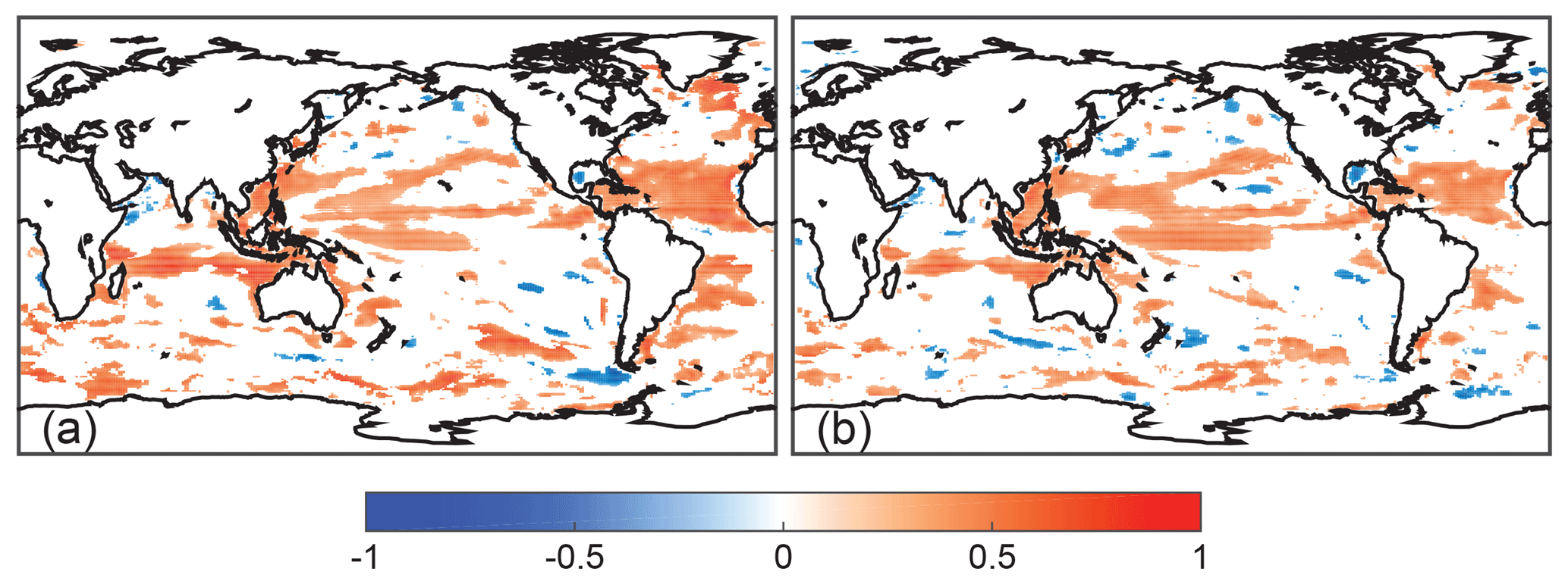
Figure 7 Air–sea CO₂ flux predictive skill, as indicated by the correlation coefficient of air–sea CO₂ flux (a) anomalies, and (b) linearly detrended anomalies from the CESM-DPLE initialized forecast in year 1 with the Landschützer et al. (2016) observational product over 1995–2015. Correlation coefficients that are not statistically significant at the 95 % level using a t test are assigned a value of zero.

As the large predictability in ΔpCO₂ is caused by the predictability of surface ocean pCO₂ in our model framework (i.e., atmospheric CO₂ concentration is prescribed rather than predicted), we next investigate the drivers of interannual predictability in surface ocean pCO₂: dissolved inorganic carbon (DIC), alkalinity (Alk), temperature (T), and salinity (S). We use a similar approach as for CO₂ flux, but here the sensitivities are derived from carbonate chemistry approximations (Doney et al., 2009; Long et al., 2013; Lovenduski et al., 2007), and all drivers are scaled to pCO₂ units (µatm) for ease of comparison:

$$\begin{array}{}\text{(4)}& {\displaystyle }{\displaystyle }r\cdot {\displaystyle \frac{\partial p{\mathrm{CO}}_{\mathrm{2}}}{\partial x}}\cdot {\mathit{\sigma }}_x.\end{array}$$

The surface ocean pCO₂, and thus the air–sea CO₂ flux predictability, for forecast lead year 1 is largely driven by predictability in surface ocean DIC and Alk, with temperature playing a secondary role and salinity a minor role (Fig. 6). The similar predictability of DIC and Alk across many regions hints at an important role for ocean circulation, rather than biological productivity (which has a much larger impact on DIC than Alk), in CO₂ flux predictability.

3.2 Predictive skill

We next evaluate the predictive skill of the CESM-DPLE forecasts; the skill is a measure of the ability of the forecast to reproduce the observational record. For air–sea CO₂ flux, direct observations are rare, and we are constrained to estimates of flux from observations of sparsely sampled surface ocean pCO₂. Here, we use as our observational metric the CO₂ flux estimated from the Landschützer et al. (2016) surface ocean pCO₂ product. This product is a gap-filled estimate of surface ocean pCO₂, which, when combined with measurements of atmospheric pCO₂, sea surface temperature, salinity, and wind, yields a monthly estimate of air–sea CO₂ flux at 1^∘ × 1^∘ horizontal resolution from 1982–2015 (see also Fig. 2a). As the pCO₂ observations are rather sparse prior to 1995 (Bakker et al., 2016), we calculate skill for the period between 1995 and 2015 only, but show for the interested reader the full observational product time series.

The CESM-DPLE initialized predictions exhibit some skill at representing the globally integrated air–sea CO₂ flux in forecast lead year 1 (Fig. 3a and b; initialized forecast skill 0.88; detrended, initialized forecast skill 0.66). Our comparison indicates that CESM-DPLE (and the reconstruction, for that matter) struggles to produce the pronounced trends toward anomalous CO₂ outgassing in the 1990s and anomalous CO₂ uptake in the 2000s. The ability (or lack thereof) of ESMs to reproduce the observationally derived multi-decadal air–sea CO₂ flux variability has been the subject of recent publications (Gruber et al., 2019; Li and Ilyina, 2018), though no robust mechanisms seem to explain the (mis)match. The CESM-DPLE initialized forecast in forecast lead year 1 exhibits moderate predictive skill in the tropics and subtropics (Fig. 7) and low skill elsewhere.

3.3 Predictability and predictive skill on the biome scale

Because the predictability of air–sea CO₂ flux is primarily driven by the predictability of the biogeochemical state variables DIC and Alk, it makes sense to aggregate predictability across biogeographical biomes. We probe the limits of predictability and predictive skill in regional air–sea CO₂ flux by averaging the local flux across 17 biogeographical biomes. This is achieved by re-gridding the Fay and McKinley (2014) mean biome mask to the CESM model grid and computing the area-weighted average CO₂ flux from the reconstruction, CESM-DPLE initialized forecasts, and observationally derived pCO₂ product. The detrended CO₂ flux anomalies for three of the biomes are shown for forecast lead year 1 in Fig. 8, and the predictability and predictive skill across all biomes is detailed in Table 1. These three biomes were chosen to contrast their predictability and/or predictive skill.

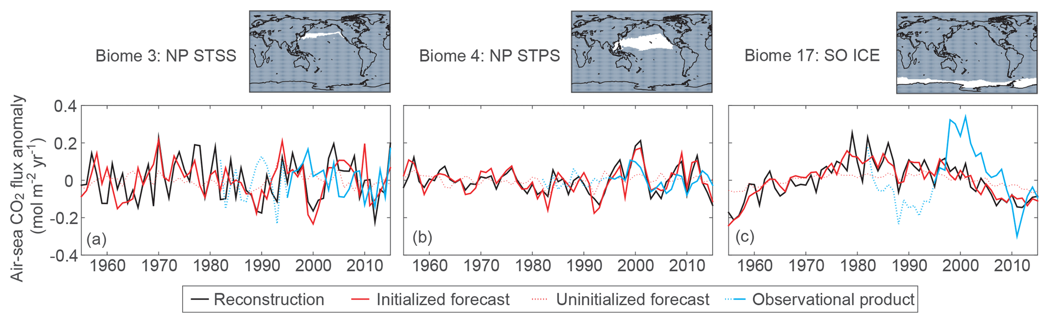
Figure 8 Temporal evolution of the biome-averaged air–sea CO₂ flux anomalies in the (a) NP STSS, (b) NP STPS, and (c) SO ICE biomes (mol m⁻² yr⁻¹). The following time series are plotted: (black) reconstruction, (red) CESM-DPLE initialized forecast, (red dotted) CESM-LE uninitialized forecast, and (blue) Landschützer et al. (2016) observationally based product. The CESM-DPLE time series is the linearly detrended, drift-corrected, ensemble mean forecast anomalies in year 1; the reconstruction, CESM-LE ensemble mean, and observed time series have been transformed to anomalies by removing the linear trend. Observations prior to 1995 are dotted due to lower observation density. Positive anomalies indicate anomalous ocean outgassing.

The biome-averaged CO₂ flux anomalies from the CESM-DPLE initialized forecast in forecast lead year 1 exhibit high correlations with the reconstruction anomalies in the North Pacific subtropical biomes and in the Southern Ocean ice biome (Fig. 8; Table 1), indicating high potential for the prediction of CO₂ flux anomalies. This predictability decreases with increasing forecast lead time in the North Pacific subtropical biomes, but persists for the Southern Ocean ice biome through forecast years 7–9 (Fig. 8). Indeed, the Southern Ocean ice biome is an anomaly in this regard; in the other 16 biomes, predictability drops off with prediction lead time (not shown).

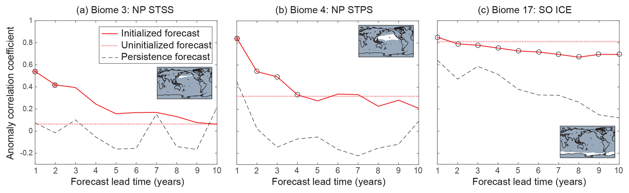
Figure 9 Predictability of biome-averaged CO₂ flux as a function of lead time in the (a) NP STSS, (b) NP STPS, and (c) SO ICE biomes, as indicated by the correlation coefficient of detrended CO₂ flux anomalies from the (red) CESM-DPLE initialized forecast and the (red dotted) CESM-LE uninitialized forecast with the reconstruction. The black dashed line shows the correlation coefficient of the persistence forecast as a function of lead time. Red asterisks (black circles) on the initialized forecast indicate predictability that is statistically different from the initialized (persistence) forecast at the 95 % level using a z test.

Initialization engenders the predictability of air–sea CO₂ flux variability the North Pacific subtropical biomes, as we find low correlation between the uninitialized CESM-LE forecast CO₂ flux anomalies and the reconstruction anomalies here (Fig. 8a and b; Table 1). The initialized forecast for these biomes has higher predictability than the uninitialized forecast and the persistence forecast for 7–8 years (Fig. 9). These conclusions hold for most of the other ocean biomes (Table 1), with a few exceptions for which the uninitialized forecast and/or persistence forecast are similar to the initialized forecast (e.g., the eastern Pacific equatorial biome). In the Southern Ocean ice biome, the CO₂ flux predictability is almost entirely driven by external forcing, and the persistence forecast indicates high predictability as well (Figs. 8 and 9, Table 1). Thus, the high and long-lasting predictability in this biome must be interpreted with caution given the importance of external forcing in predicting CO₂ flux anomalies here.

Table 1 Biome-averaged air–sea CO₂ flux statistics.

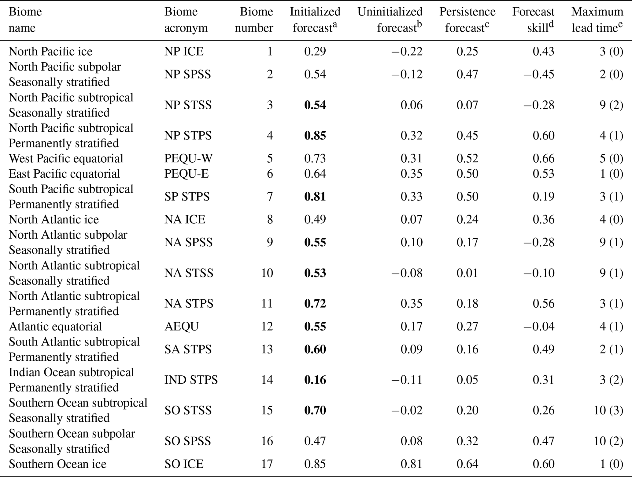
^a Correlation of CO₂ flux anomalies from the CESM-DPLE initialized forecast in lead year 1 with the reconstruction. Boldface indicates that the correlation coefficient is statistically different from both the uninitialized and persistence forecasts at the 95 % level using a z test. ^b Correlation of CO₂ flux anomalies from the CESM-LE uninitialized forecast with the reconstruction. ^c Autocorrelation of the persistence forecast at lead year 1. ^d Correlation of CO₂ flux anomalies from the CESM-DPLE initialized forecast in lead year 1 with the Landschützer et al. (2016) observational product over 1995–2015. ^e The maximum forecast lead time (years) in which the CESM-DPLE initialized forecast has both higher predictability than the uninitialized CESM-LE forecast and a higher correlation coefficient than the persistence forecast. Lead times in parenthesis account for statistical separation in correlation coefficients at the 95 % level using a z test.

The predictive skill of CESM-DPLE in forecast lead year 1 is illustrated for three biomes in Fig. 8 and Table 1. Again, we note the moderate skill in the tropics and subtropics and lower skill elsewhere.

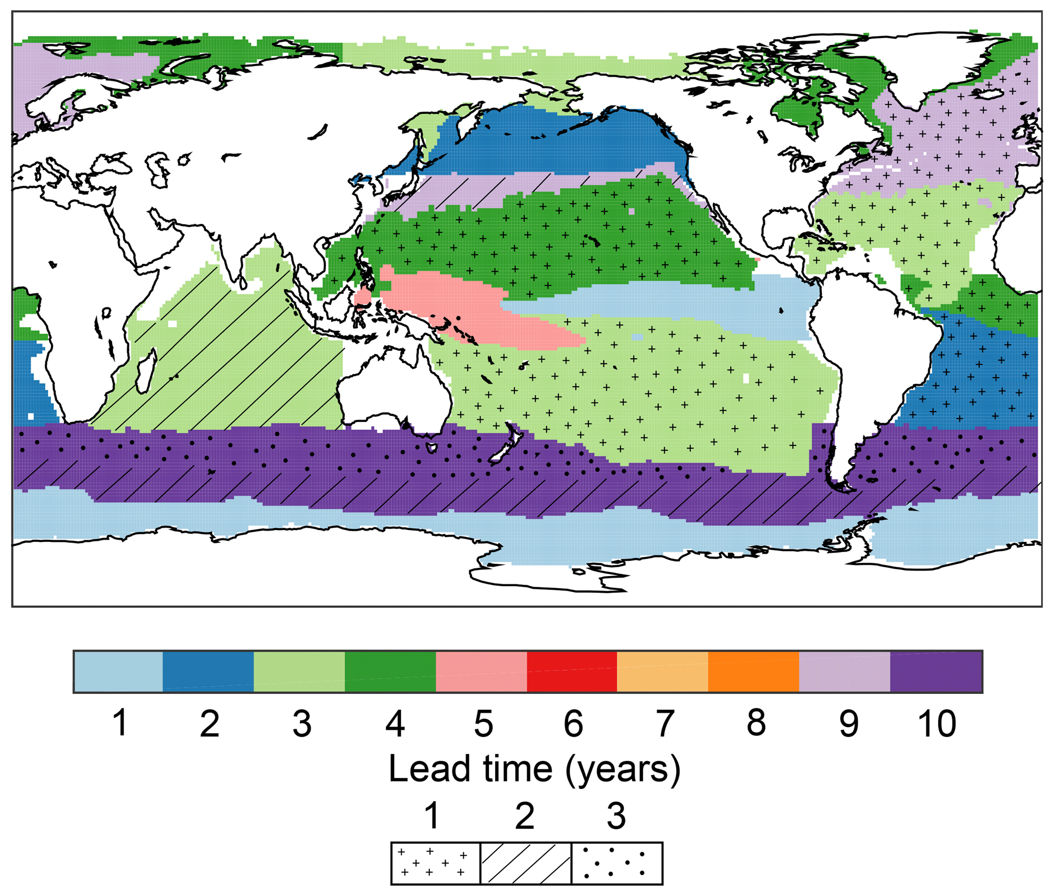
Figure 10 For each biome, the maximum forecast lead time (years) in which the initialized CESM-DPLE CO₂ flux forecast has both higher predictability than the uninitialized CESM-LE forecast and a higher correlation coefficient than the persistence forecast. Hatching shows the maximum forecast lead time while accounting for statistical separation of correlation coefficients at the 95 % level using a z test.

The difference in the predictability between the initialized, uninitialized, and persistence forecasts reveals the impact of initialization on predictions of air–sea CO₂ flux variability on the biome scale (Fig. 9). We probe the limits of initialized predictability in each biome by calculating the maximum forecast lead time for which the initialized CESM-DPLE CO₂ flux forecast has both higher predictability than the uninitialized CESM-LE and persistence forecasts and present the results in Fig. 10. Our results indicate that initialization improves the forecast for the longest lead times in the subantarctic Southern Ocean and the northern North Atlantic, where the initialized forecast beats the other two forecasts out to forecast lead times of 10 and 9 years, respectively. We note, however, that the improvement in the North Atlantic is only statistically significant for 1 lead year and in the Southern Ocean for 2–3 lead years. Given the important role of these two regions for the global ocean uptake of anthropogenic carbon, and the numerous studies linking climate variability to air–sea CO₂ flux variability in these regions, this long-lasting predictability is encouraging. In other regions, however, such as the Southern Ocean ice or eastern equatorial Pacific biomes, the initialized forecast only beats the uninitialized or persistence forecast for a single year, indicating little benefit of forecast initialization for CO₂ flux forecasts here.

4 Conclusions

We analyze output from the CESM-DPLE system to quantify and understand the sources of predictability and predictive skill in global and regional air–sea CO₂ flux on annual to decadal timescales. We find high potential predictability in globally integrated CO₂ flux several years in advance that is engendered by initialization. This potential predictability is evident across much of the global ocean, driven by predictability in ΔpCO₂, which itself is primarily driven by predictability in surface ocean DIC and Alk. While the CESM-DPLE system exhibits strong potential predictability, model skill as compared to an observationally based product remains a challenge to developing useful forecasts.

Our study complements two recent studies of ocean carbon decadal predictions conducted at different modeling centers. Li et al. (2016) use decadal predictions from MPI-ESM to investigate near-term changes in North Atlantic CO₂ flux, while Séférian et al. (2018) use CNRM-ESM1 to assess the predictability horizon of globally integrated ocean and land carbon fluxes. While these studies use different prediction systems, we nevertheless come to some of the same conclusions. For example, Séférian et al. (2018) find that global ocean carbon uptake is potentially predictable for up to 6 years, and Li et al. (2016) find high potential predictability in the North Atlantic that is engendered by initialization. These studies collectively suggest predictability for near-term ocean carbon uptake on global and regional scales, which is beneficial for forecasting the future global carbon budget and climate system.

While the ever-expanding field of decadal climate prediction has the potential to inform policy and management decisions moving forward, decadal forecasts come with several caveats. Initialization shock and drift of the coupled model system, the inability of Earth system models to realistically simulate internal variability, uncertain future levels of radiative forcing, and imperfect observations are frequently cited as limitations to making accurate forecasts of the future (Meehl et al., 2014). In the case of ocean carbon, it is important to note that potential predictability in regional CO₂ flux may be driven by initialization of the physical (e.g., SST) or biogeochemical (e.g., DIC) ocean state (Li et al., 2016) and that the spatiotemporal coverage of CO₂ flux observations is insufficient to fully address predictive skill in our forecast systems.