Amplification of ENSO-driven vegetation variability at decadal and longer timescales

The El Niño-Southern Oscillation (ENSO) is recognized as the dominant driver of global vegetation variability on interannual timescales. Here, we examine how ENSO affects decadal to multi-decadal vegetation variability. We address this with partial spectral and mediation analysis applied to multi-centennial pre-industrial control simulations from 11 CMIP6 models with dynamic leaf area index (LAI). We find a spectral reddening of ENSO-driven vegetation variability, with a 20 %–25 % amplification of the LAI signal at multi-decadal timescales and a 25 %–65 % reduction at interannual timescales. This amplification is primarily concentrated in tropical hotspots, such as the northern Amazon and Southeast Asia, which dominate the global gain signal. The coherence between ENSO and LAI at these multi-decadal timescales is largely governed by a direct pathway (88 %), while the Pacific Decadal Oscillation (PDO) only acts as a weak mediator (12 %). In contrast, the Atlantic Multidecadal variability (AMV) exhibits significant multi-decadal coherence with vegetation but lacks the associated spectral reddening. Mechanistically, ENSO-driven LAI persistence originates from ENSO-induced changes in near-surface soil moisture, which is subsequently amplified by vegetation dynamics. This ENSO-related memory also manifests in Gross Primary Production (GPP), but it is suppressed in Net Primary Production (NPP) by a compensatory increase in autotrophic respiration. Our results illustrate how terrestrial persistence acts as a predictable, non-oceanic source of decadal variability, which could help extend the skill of climate predictions and improve hydrological risk management.

1 Introduction

The terrestrial biosphere plays a multifaceted role in regulating the global climate system. As the physical interface between the atmosphere and land surface, vegetation fundamentally controls global water and energy cycles by modifying surface albedo and regulating the partitioning of heat and water fluxes (Bonan, 2008). Furthermore, the terrestrial biosphere is a critical component of the global carbon cycle, absorbing approximately one-third of current anthropogenic carbon dioxide emissions (Friedlingstein et al., 2025). Due to this central importance, understanding how vegetation structure, measured by proxies such as leaf area index (LAI), and associated carbon flux metrics respond to climate variability is essential.

Short-term climate variability (monthly to interannual) can strongly influence ecosystem processes, serving as important indicators of ecosystem vulnerability and resilience (Seddon et al., 2016; Thornton et al., 2014). The largest driver of this terrestrial variability on interannual timescales is the El Niño–Southern Oscillation (ENSO) (McPhaden et al., 2006; Timmermann et al., 2018; Zhao et al., 2018; Catalano et al., 2016). ENSO induces changes in ecosystem structure and plant productivity, particularly over Australia, South America, Africa, and southern Asia (Buermann et al., 2002; Woodward et al., 2008). Beyond these direct structural effects, ENSO also modulates the interannual variability of vegetation resilience, thereby influencing not only the immediate vegetation response but how readily the biosphere returns to its baseline state following an ENSO event (Zhou et al., 2025). ENSO-driven vegetation variability directly controls the interannual fluctuations in the terrestrial carbon flux, acting as the dominant source of variability in the global carbon cycle (Wang et al., 2013; Zhang et al., 2018). These ENSO-induced vegetation changes are primarily governed by atmospheric teleconnections that modulate regional temperature and precipitation patterns (e.g., Alessandri and Navarra, 2008; Catalano et al., 2016). These regional anomalies then impact vegetation dynamics by altering environmental factors determining vegetation productivity, such as soil moisture and surface radiation. However, the land surface is not merely a passive recipient of this variability: vegetation dynamics and soil moisture have been shown to create delayed biophysical feedbacks on precipitation patterns, thereby acting as interannual memory of ENSO events (Alessandri and Navarra, 2008; Catalano et al., 2016). Modeling studies have demonstrated that vegetation dynamics can actively introduce and enhance decadal variability in temperature and precipitation over land (Wang and Eltahir, 2000; Delire et al., 2011; Wang et al., 2011). However, these studies primarily focused on vegetation's feedback on climate variability and did not assess how these vegetation changes are modulated or driven by ocean-atmosphere variability (the ultimate driver of much climate variability) in the first place.

While interannual ENSO-vegetation links are well-studied, much less is known about the impact of slower, decadal-scale climate variability on terrestrial biosphere variability. ENSO itself exhibits decadal modulations in its characteristics (Zhang et al., 1997; Wittenberg, 2009; Sun and Yu, 2009), but other key low-frequency climate modes, such as the Pacific Decadal Oscillation (PDO) and the Atlantic multidecadal variability (AMV), also operate on longer timescales (Deser et al., 2010). The PDO in particular has been suggested to be closely linked to the low-frequency (decadal and multi-decadal) modulations of ENSO (Zhang et al., 1997; Newman et al., 2016; Wills et al., 2019). While the AMV is largely independent of ENSO (Zhang et al., 2019), it has been found to modulate multi-decadal ENSO variance through tropical Atlantic sea surface temperature (SST) changes and the resulting shifts in the Walker circulation (Dong et al., 2006; Levine et al., 2017). Given the fundamental influence of these oceanic modes on the global climate, it is reasonable to assume that they also lead to variations in vegetation dynamics. Recent studies have begun to explore this relationship, demonstrating that these decadal climate modes exert a significant control on long-term variability in vegetation and the terrestrial carbon cycle. For instance, Lu et al. (2023) showed using satellite data and EC-Earth3 simulations that the ENSO, PDO, and AMV changes together explain approximately 20 % of global decadal LAI variability, with regional contributions reaching up to 40 %. On the carbon flux side, studies using ecosystem models found that the PDO and AMV strongly influence decadal to multi-decadal carbon flux anomalies (Ito, 2011; Zhang et al., 2018). Specifically, Zhang et al. (2018), using spectral analysis, found that multi-decadal variability in net biome productivity in tropical rainforests is modulated by the PDO's influence on temperature and precipitation. Furthermore, Park et al. (2020) used long pre-industrial control (piControl) simulation from a fully-coupled large ensemble model (CESM1-LE) to demonstrate that decadal ENSO-like variability accounts for a substantial fraction (around 36 %) of decadal variability in global land carbon fluxes.

Despite these previous studies, significant limitations persist in our understanding of decadal climate–vegetation coupling (Linscheid et al., 2020). Methodologically, many of these efforts relied on transient historical simulations in ecosystem models (Zhang et al., 2018; Ito, 2011) or a single Earth System Model (ESM) (Lu et al., 2023), hindering the rigorous isolation of intrinsic climate-vegetation memory from the confounding effects of long-term forcing, such as climate change and related CO₂ fertilization. These studies have also generally employed conventional correlation or regression analysis (Ito, 2011; Lu et al., 2023; Park et al., 2020), which cannot fully disentangle causal and lagged relationships (Wu et al., 2015). This is particularly problematic for the closely related ENSO and PDO signals on decadal timescales (Wills et al., 2018), hindering the rigorous quantification of direct versus mediated effects of ENSO on vegetation. Additionally, frequency-resolved assessment would help to understand whether and how vegetation processes modify the amplitude of ENSO-driven variability at different timescales over land. For example, this analysis would allow quantification of “spectral reddening” in the biosphere, a process where persistence or memory of previous anomalies leads to relatively larger variations at lower frequencies and longer periods compared to higher frequencies. Understanding reddening can help to reveal whether the biosphere merely passively responds to low-frequency atmosphere-ocean variability or actively facilitates an amplification of low-frequency ENSO-driven vegetation variability by shifting power to decadal and longer timescales. Finally, while studies have assessed variability in net carbon products (Ito, 2011; Zhang et al., 2018; Park et al., 2020), the mechanistic link demonstrating how long-term memory signal in vegetation changes is related to carbon fluxes is incomplete.

To address these gaps, our study systematically investigates the decadal and multi-decadal influence of ENSO, the PDO and the AMV on variability in global vegetation using long-term piControl simulations from multiple CMIP6 ESMs with interactive LAI. We apply advanced time series analysis techniques, including spectral analysis to understand the coherence of vegetation variability with oceanic variability as well as partial spectral and mediation analysis to robustly quantify the causal pathways among ENSO, PDO, AMV, LAI, and other land-surface anomalies. Our research is guided by four core questions: (1) Is there a low-frequency amplification of ENSO-driven vegetation variability globally and regionally? (2) What is the impact of the PDO and AMV on LAI variability on decadal and multi-decadal timescales? (3) What is the dominant physical process through which ENSO-induced memory in LAI is established? (4) Does the LAI memory manifest in memory in ecosystem carbon fluxes (GPP and NPP)? Answering these questions is critical because the terrestrial memory of multi-decadal climate signals could prove to be a fundamental source of long-term memory in the Earth system. This frequency-dependent coupling between the land surface and atmosphere-ocean variability could then be leveraged as a source of predictability in decadal climate predictions.

2 Data and methods

2.1 Pre-industrial climate simulations from CMIP6

To isolate and analyze the low-frequency variability of the coupled ocean-atmosphere-land-vegetation system, we utilize single piControl realisations from 11 ESMs participating in the Coupled Model Intercomparison Project Phase 6 (CMIP6) (Eyring et al., 2016). The selected ESMs are: ACCESS-ESM1-5 (Ziehn et al., 2020), CanESM5 (Swart et al., 2019), CMCC-ESM2 (Lovato et al., 2022), CESM2 (Danabasoglu et al., 2020; Lawrence et al., 2019), EC-Earth3-Veg (Doscher et al., 2022), GFDL-ESM4 (Dunne et al., 2020), IPSL-CM6A-LR (Boucher et al., 2020), MIROC-ES2L (Hajima et al., 2020), MPI-ESM1-2-LR (Mauritsen et al., 2019; Reick et al., 2013), NorESM2-LM (Seland et al., 2020; Lawrence et al., 2019), and UKESM1-0-LL (Sellar et al., 2019; Clark et al., 2011). These models were chosen as they simulate interactive LAI in the piControl and historical runs (i.e., allowing the terrestrial biosphere to dynamically respond to simulated internal climate variability) and since they have output for LAI, NPP and GPP. Other CMIP6 ESMs with static vegetation, where LAI is fixed apart from a seasonal cycle, were excluded as they cannot capture the response to low-frequency climate variability.

Nonetheless, the representation of vegetation dynamics differs between the 11 models chosen. In eight models (CanESM5, CMCC-ESM2, CESM2, EC-Earth3-Veg, GFDL-ESM4, IPSL-CM6A-LR, MPI-ESM1-2-LR, UKESM1-0-LL) the fully interactive vegetation module is switched on, allowing for potential two-way feedbacks between changes in LAI and climate. Specifically, climate and its variability impact LAI by governing the availability of water, light, and thermal energy required for photosynthesis and phenology, while LAI in turn can modify the climate via changes in albedo, evapotranspiration, and aerodynamic roughness. However, only two models (GFDL-ESM4 and UKESM1-0-LL) explicitly model changes in the fractional coverage of Plant Functional Types (PFTs) in piControl, while the PFT distribution is fixed at 1850 levels for the remaining models.

For robust analysis of low-frequency variability, the first 500 years of available monthly data from each model's piControl run were used. This duration was chosen since it represents the minimum common length available across the selected ESMs. The terrestrial variables analyzed include:

• Leaf Area Index (LAI): A key structural variable representing the total one-sided leaf area per unit ground area. LAI is controlled by relatively slow, model-dependent processes such as phenology, allocation (partitioning of assimilated carbon into different vegetation carbon pools), and growth, making it a suitable indicator for long-term vegetation memory.

• Gross Primary Production (GPP): The total carbon mass flux fixed by plants through photosynthesis.

• Net Primary Production (NPP): The net carbon accumulation by plants, calculated as the difference between GPP and Autotrophic Respiration (R_A): $\text{NPP}=\text{GPP}-R_{\mathrm{A}}$.

Prior to all analysis, the seasonal (3-monthly) anomalies were calculated from monthly data with respect to the climatological seasonal cycle and then linearly detrended to remove any residual long-term drift in the piControl simulations. All model output was remapped to a common 2.5°×2.5° resolution using conservative remapping to facilitate multi-model comparison. The analyses, including regression and power spectral analysis, were first performed on individual model output before the multi-model ensemble mean (MEM) was computed. Model agreement was assessed by identifying grid cells where at least 9 of the 11 models agree on the sign of the calculated change (90 % confidence based on a two-sided binomial test).

2.2 Regression of vegetation dynamics onto oceanic variability

Our analysis focuses on the impact of three major oceanic modes, namely ENSO, the PDO and AMV, on changes in vegetation variability. To analyse changes related to ENSO, we use the Niño3.4 SST index which is calculated as the area-weighted average of detrended seasonal SST anomalies over the central equatorial Pacific (5° S–5° N, 190–240° E) for each CMIP6 model and the observational data (Sect. 2.3). We also examine the influence of the PDO as a mediator from ENSO variability to vegetation changes. The PDO index is calculated as the first principal component (PC1) of the detrended, seasonal SST anomalies over the North Pacific (20–70° N) (Mantua et al., 1997). Additionally, we test the impact of the AMV on LAI where the AMV index is calculated as the area-weighted average of detrended seasonal SST anomalies over the North Atlantic (0–60° N, 80° W–0 °). We note that we do not include a separate analysis of the Interdecadal Pacific Oscillation (IPO) since it has been shown that the IPO is not a distinct mode of Pacific SST variability but rather a blend of decadal-modulations of ENSO, the PDO, AMV and externally forced warming (Tung et al., 2019).

We use linear regression to quantify the spatial pattern and strength of the influence of these two oceanic modes on terrestrial variables (LAI, GPP, NPP). We calculate the regression coefficient r using the multi-dimensional dot product, which efficiently calculates the covariance across the time dimension:

$$\begin{array}{}\text{(1)}& r\left(x\right)={\displaystyle \frac{\mathrm{1}}{n-\mathrm{1}}}v(t,x)\cdot I_{\text{norm}}\left(t\right)\end{array}$$

where n is the length of the time series, v(t,x) is the terrestrial variable and I_norm(t) the oceanic index normalised by its standard deviation. The resulting regression coefficient map r(x) then represents the spatial pattern of change in the terrestrial variable v associated with a one-standard-deviation change in the oceanic index I_norm. Note that we use the notation of regression of variable Y on variable X (i.e., LAI regressed on Niño3.4 index) throughout the text.

To visualize the time evolution of the vegetation response associated with the oceanic mode, we compute an associated time series (T_V) for the vegetation variable. This time series is obtained by projecting the gridded vegetation anomalies onto the calculated regression map r(x):

$$\begin{array}{}\text{(2)}& T_{\mathrm{V}}\left(t\right)=v_{\mathrm{w}}(t,x)\cdot r\left(x\right)\end{array}$$

where v_w is the vegetation anomaly v weighted by the cosine of the latitude. Finally, the T_V time series is normalized by its standard deviation to allow for comparisons across different terrestrial variables and models, and subscript V will be replaced by LAI, GPP, or NPP depending on the terrestrial variable used. This resulting time series represents the component of global vegetation variability linearly co-varying with the oceanic index across the full timeseries, similar to other standard pattern-extraction techniques like Maximum Covariance Analysis. Importantly, because the regression map r(x) is strictly constant in time, this methodology does not impose any explicit constraints or a priori assumptions on the temporal evolution or frequency profile of T_V(t). The frequency content is inherited entirely from the underlying, time-dependent vegetation anomalies v_w(t,x). Consequently, frequency-domain features, like spectral reddening or a multi-decadal gain greater than 1, reflect the dynamical response of the terrestrial system rather than artefacts of the index construction.

2.3 Historical data from CMIP6, observations and satellites

To validate the relationship between oceanic variability and vegetation dynamics found in the piControl simulations, we analyze historical CMIP6 simulations and satellite-based observations over the common historical period of 1982–2014. This period is chosen for consistency with the availability of both satellite vegetation data and the CMIP6 historical runs (Eyring et al., 2016). However, it should be noted that this time period is significantly shorter than the 500 years of simulations used for the piControl-based analysis, which hinders an analysis of variability longer than 30 years. Additionally, it should be noted that this comparison focuses on the spatial consistency of the internal ENSO-vegetation coupling, acknowledging that the historical record also incorporates transient anthropogenic greenhouse gas and land use signals that are absent in the control simulations.

We use historical CMIP6 data for SST (to calculate Niño3.4), LAI, GPP and NPP from the same 11 ESMs remapped to 2.5°×2.5°. To compare these simulated relationships to observed ones, we used the Niño3.4 SST index from the HadISST1.1 product (Rayner et al., 2003) and monthly data for LAI, GPP and NPP from the Global Land Surface Satellite (GLASS) mission (Liang et al., 2021, 2023). The GLASS dataset, which is a product of the AVHRR multi-sensor data, was selected as it provides data for all three vegetation variables and temporal alignment with the CMIP6 historical period. The GLASS LAI product has been shown to provide high-quality and high-precision global long-term data, which has been validated against in situ measurements and intercompared with other satellite products (Liang et al., 2021; Li and Xiao, 2020). As described in Sect. 2.2, a regression analysis between the seasonal Niño3.4 and the seasonal vegetation indices was performed using the detrended historical CMIP6 simulations in comparison to the detrended observational data.

2.4 Mediation analysis

In order to study the causal pathway from variability in ENSO to LAI, we employ a mediation analysis framework, following the methodology established by MacKinnon et al. (2000) and later used by Kolstad and O'Reilly (2024) and Kolstad (2026) to study climate variability. In line with this literature, we use “causal” to describe a statistical relationship in which the direction of influence is established by a systematic causal inference methodology. Here, the Niño3.4 index is defined as the predictor or independent variable (X), and LAI regressed on Niño3.4 (T_LAI) is the dependent or outcome variable (Y) (Fig. 1). Mediation analysis then allows us to test the influence of the PDO (variable Z= PDO index), which is closely linked to the low-frequency modulations of ENSO, as a mediator of the relationship between ENSO and LAI. Specifically, we investigate whether simulated low-frequency coherence between LAI and the PDO are solely due to the coherence between ENSO and the PDO, which is then transmitted by the PDO to LAI, or if a direct causal relationship exists between ENSO and LAI at low frequencies even after accounting for the PDO's influence.

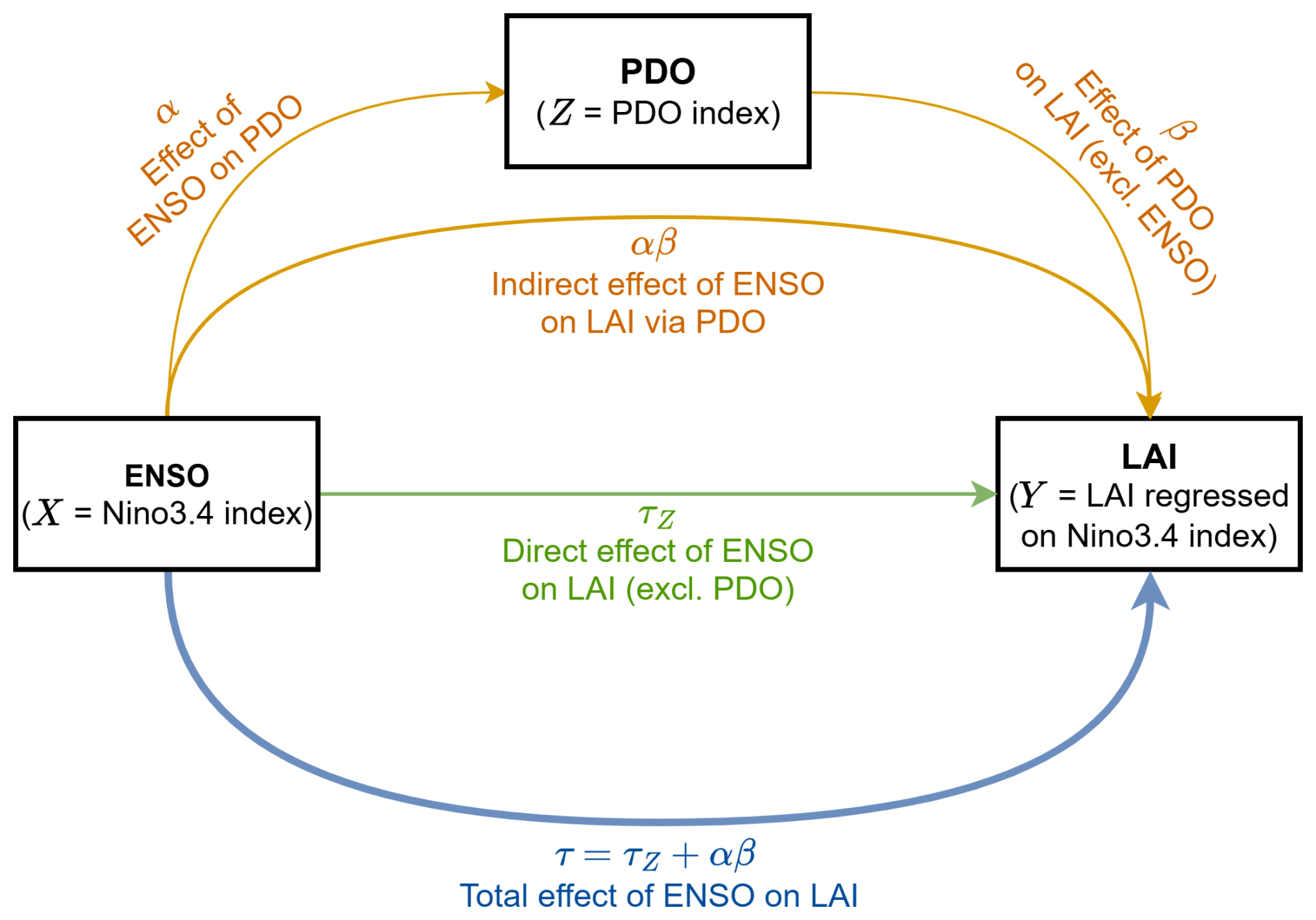
Figure 1 Schematic diagram illustrating the total and direct effect of ENSO on LAI and the indirect effect via the PDO. The coefficients τ and τ_z denote the total and direct effects of ENSO on LAI, respectively. The indirect effect α⋅β is quantified by the product of α (effect of ENSO on PDO) and β (effect of PDO on LAI, excluding the linear influence of ENSO). Schematic adapted from Kolstad and O'Reilly (2024).

The relationships are examined using the following set of linear regression equations, omitting intercepts and residuals for clarity. The total effect of the predictor X on the outcome Y is given by the regression coefficient τ:

$$\begin{array}{}\text{(3)}& Y=\mathit{\tau }X.\end{array}$$

This total effect τ comprises both the direct effect τ_Z from ENSO to LAI (X→Z), excluding the influence of the PDO, and the indirect (mediated) pathway via the PDO ($X\to Z\to Y$) (Fig. 1).

The direct effect of the predictor X on the outcome Y, while excluding the effect of the mediator Z, is represented by the coefficient τ_Z. The influence of the mediator Z on the outcome Y, when excluding the effect of the predictor X, is given by the coefficient β. Thus, Y can be predicted by:

$$\begin{array}{}\text{(4)}& Y={\mathit{\tau }}_{Z}X+\mathit{\beta }Z.\end{array}$$

Additionally, the influence of the predictor X on the mediator Z is calculated by the coefficient α:

$$\begin{array}{}\text{(5)}& Z=\mathit{\alpha }X.\end{array}$$

The portion of the total effect that is mediated (indirect effect) can then be calculated as the product of the path coefficients α and β. This indirect effect is also equivalent (up to differences in regression residuals) to the difference between the total and direct effects: $\mathit{\alpha }\mathit{\beta }=\mathit{\tau }-{\mathit{\tau }}_Z$.

According to the criteria for mediation from Baron and Kenny (1986), the coefficients τ, α, and β must be significantly different from zero. Furthermore, τ and τ_Z must have the same sign, as the mediation is inconsistent otherwise.

The role of the mediator Z can be categorized based on the magnitude and significance of the direct effect τ_Z:

• Perfect mediator: Z fully accounts for the relationship X→Y if τ_Z is not significantly different from zero.

• Partial mediator: Z partially explains the relationship X→Y if τ_Z is significantly different from zero, but its magnitude is less than the total effect ($\left|{\mathit{\tau }}_Z\right|<\left|\mathit{\tau }\right|$).

• Suppressor: The relationship X→Y is stronger when Z is accounted for, which is given by τ_Z being significantly different from zero and its magnitude being greater than the total effect ($\left|{\mathit{\tau }}_Z\right|>\left|\mathit{\tau }\right|$).

Finally, it should be mentioned that the presence of mediation or suppression by Z does not necessarily imply that Z is the sole mediator or suppressor of the effect of X on Y, nor does it on its own establish the causal direction of the relationships.

Since we are interested in decadal to multi-decadal influence of ENSO on LAI, a 10-year low-pass filter is applied to all three variables (i.e., Niño3.4 index, PDO index and LAI regressed on Niño3.4) prior to the mediation analysis. Note that these filtered indices capture decadal modulations of these variables rather than representing independent climate modes. We then perform the regressions outlined in Eqs. (3)–(5) for each model individually. This yields the direct effect (τ_Z), the indirect effect via the PDO (αβ), and the total effect (τ) for each model. The multi-model mean is then calculated as the mean across these model-specific coefficients.

2.5 Spectral analysis of vegetation dynamics

We also perform analysis in the frequency domain to quantify the frequency-dependent relationships. We firstly calculate the power spectral density of the Niño3.4 index and vegetation variable regressed on Niño3.4 using Welch's method to analyse spectral reddening (Welch, 2003). The presence of enhanced power at longer periods in the spectrum of the LAI time series associated with the ENSO-driven component (i.e., T_V from Eq. 2) would provide key evidence for LAI translating the low-frequency ENSO signal into a multi-decadal vegetation response.

In order to quantify this reddening and determine spectral properties like coherence, gain, and phase between Niño3.4 and vegetation variables, we use the multi-taper method (MTM; Thomson, 1982; Percival and Walden, 1993; Ghil et al., 2002). MTM is a robust technique for the time-frequency analysis of signals that employs a set of orthogonal tapers, known as Discrete Prolate Spheroidal Sequences (DPSS) or Slepian functions. These multiple orthogonal tapers (DPSS) provide several statistically independent spectral estimates from the same data segment, significantly reducing the variance compared to single-taper methods. Without the use of tapers, the spectral analysis of finite time series is susceptible to spectral leakage, where power from one frequency band artificially spreads into others.

2.5.1 Multi-taper spectra calculation

To perform the multi-taper spectral analysis, we first detrend the timeseries x(t) and y(t) of length n and sampling interval dt and then remove their respective means. As mentioned before in Sect. 2.4, we focus on ENSO (given by the Niño3.4 index) as predictor x(t) and vegetation variables like LAI, GPP and NPP regressed on Niño3.4 as outcomes y(t). We then determine the number of orthogonal tapers for spectral averaging as $K=\mathrm{2}\cdot \text{NW}-\mathrm{1}$ using the time-bandwidth product NW of 8, which gives 15 orthogonal tapers. Commonly, NW is chosen to be 2 or 4 for shorter datasets, while longer datasets can use greater NW while still maintaining the required frequency resolution (Ghil et al., 2002).

We then compute F_kx(f) and F_ky(f) by multiplying each timeseries by the tapering function (k) and transforming the signal into the frequency domain using discrete Fourier transforms. The auto-spectra S_xx(f) and S_yy(f) as well as the cross-spectra S_xy(f) between time series x and y at frequency f can then be computed following Eqs. (6)–(8), where F^* denotes the complex conjugate of F.

$$\begin{array}{}\text{(6)}& {\displaystyle }{S}_{xx}\left(f\right)=\sum _{k=\mathrm{1}}^K{F}_{kx}\left(f\right)F_{kx}^{*}\left(f\right)\text{(7)}& {\displaystyle }{S}_{yy}\left(f\right)=\sum _{k=\mathrm{1}}^K{F}_{ky}\left(f\right)F_{ky}^{*}\left(f\right)\text{(8)}& {\displaystyle }{S}_{xy}\left(f\right)=\sum _{k=\mathrm{1}}^K{F}_{kx}\left(f\right)F_{ky}^{*}\left(f\right)\end{array}$$

2.5.2 Coherence and gain calculation

Based on these spectra, we compute the transfer function:

$$\begin{array}{}\text{(9)}& H\left(f\right)={\displaystyle \frac{S_{xy}\left(f\right)}{S_{xx}\left(f\right)}},\end{array}$$

which describes the direct linear frequency-domain relationship between the predictor series x and the outcome series y (x→y).

The gain G(f) is then given by the magnitude of the transfer function H(f):

$$\begin{array}{}\text{(10)}& G\left(f\right)=\left|H\right(f\left)\right|.\end{array}$$

Gain values can be interpreted as the ratio of the magnitude of variability in the output signal to the magnitude of variability in the input signal (for instance, how many units of LAI variability are produced by a unit of ENSO variability at a certain frequency). If the gain increase in magnitude as frequency decreases/period increases, this indicates a reddening effect which can be characterised by the spectral slope of the gain. When the variables are normalised, a gain greater than 1 signifies an active amplitude amplification of the forcing signal at that timescale relative to other timescales.

The coherence squared C²(f) is a measure of the linear correlation (squared) between two signals in the frequency domain (e.g., Carter, 1987):

$$\begin{array}{}\text{(11)}& C^{\mathrm{2}}\left(f\right)={\displaystyle \frac{\left|S_{xy}\right(f){|}^{\mathrm{2}}}{S_{xx}\left(f\right)S_{yy}\left(f\right)}}.\end{array}$$

Coherence quantifies the fraction of the power of y that can be linearly predicted by x at each frequency and varies between 0 and 1. We assessed the statistical significance of the estimated coherence by determining the critical coherence threshold using phase randomisation (Ebisuzaki, 1997). This method involves generating a large ensemble (here 500) of surrogate time series for the input (Niño3.4 index) by randomizing the phase spectrum while preserving the amplitude spectrum of the original data. The critical coherence is then defined as the 90 percentile of the coherence squared values calculated between the surrogate Niño3.4 index and the original response variable (e.g. LAI regressed on Niño3.4). Phase randomization has the advantage of preserving the spectral properties of the resampled timeseries.

The phase spectrum Φ(f) provides the phase lag or lead of output signal relative to the input signal and is calculated as the angle of the cross-spectrum:

$$\begin{array}{}\text{(12)}& \mathrm{\Phi }\left(f\right)=\mathrm{\angle }\left(S_{xy}\right(f\left)\right).\end{array}$$

Positive phase (negative) values indicate that y lags (leads) x. Additionally, it should be noted that the lead/lag time associated with phase values is period-dependent. For instance, a lag of 45° in the 2–4 year period band would indicate a delay of 3–6 months.

2.5.3 Partial spectral analysis

We use a partial spectral analysis method to isolate the linear relationship between the two time series x and y in the frequency domain, while removing the linear influence of a mediator variable z (for a pathway $x\to z\to y$) (e.g., Rosenberg et al., 1989). Here, x is given by the Niño3.4 index, y is given by LAI regressed on the Niño3.4 index and z is given by the PDO index. This allows us to test the influence of the PDO as a mediator from ENSO to LAI as the PDO is closely linked to the low-frequency modulations of ENSO (Zhang et al., 1997; Newman et al., 2016; Wills et al., 2019). Additionally, we use this partial spectral analysis to examine the mechanistic pathway by which ENSO variability can impact LAI, for instance via changes in radiation, soil moisture, temperature or net precipitation. As before, these variables were deseasonalised and linearly detrended.

Previous studies analyzing mediation pathways usually relied on methods like the mediation method described in Sect. 2.4 (MacKinnon et al., 2000; Kolstad and O'Reilly, 2024; Kolstad, 2026) or Granger causality (e.g., Le, 2023; McGraw and Barnes, 2018). Partial spectral analysis provides additional information in comparison to mediation or Granger causality analysis: (1) It allows an investigation of the timescales of relationships (e.g., annual, decadal, and multi-decadal) directly by decomposing the relationship by frequency. (2) It captures lead-lag relationships precisely using the phase information. This lead-lag information is helpful to determine the direction of influence between two variables, whereas physical reasoning is needed to argue for the direction of the feedback in the mediation method. (3) It provides a way to quantify reddening by examining the spectral slope of the gain, indicating whether the primary variable of interest or a mediating variable act as a low-pass filter, shifting variability from higher to lower frequencies. The partial spectra method has been used extensively in neuroscience (e.g., Sun et al., 2004; Medkour et al., 2009; Makhtar et al., 2020; Dodson-Robinson and Haley, 2025) and seismology (e.g., White, 1984; Gibbons et al., 2008), but to our knowledge has not been applied to disentangle frequency-specific causal links in climate science.

Partial spectral analysis is based on conditional auto- and cross-spectra. First, we determine the conditional auto-spectra S_xx|z and S_yy|z (Rosenberg et al., 1989), which give the auto-spectra of x and y, respectively, having removed the linear influence of z (denoted as |z) as

$$\begin{array}{}\text{(13)}& S_{xx|z}=S_{xx}-{\displaystyle \frac{|S_{xz}{|}^{\mathrm{2}}}{S_{zz}}}\end{array}$$

and

$$\begin{array}{}\text{(14)}& S_{yy|z}=S_{yy}-{\displaystyle \frac{|S_{yz}{|}^{\mathrm{2}}}{S_{zz}}}.\end{array}$$

Similarly, the conditional cross-spectra S_xy|z can be calculated as

$$\begin{array}{}\text{(15)}& S_{xy|z}=S_{xy}-{\displaystyle \frac{S_{xz}{S}_{zy}}{S_{zz}}}.\end{array}$$

Note that we omit the explicit notation of the frequency dependence in Eqs. (13)–(20) for better readability.

The partial transfer function H_xy|z is calculated using the conditional spectra as

$$\begin{array}{}\text{(16)}& H_{xy|z}={\displaystyle \frac{S_{xy|z}}{S_{xx|z}}},\end{array}$$

with its magnitude giving the partial gain G_xy|z

$$\begin{array}{}\text{(17)}& G_{xy|z}=\left|H_{xy|z}\right|.\end{array}$$

To find out if z is a perfect or partial mediator, we first calculate the direct transfer function H_xy|z and the mediated component $H_{xz}\cdot H_{zy|x}$ over a certain period. Because these are complex-valued, their relative phase must be considered by performing the addition in the complex domain. The magnitude of the sum of the direct and mediated transfer function then yields the reconstructed total gain:

$$\begin{array}{}\text{(18)}& G_{xy}=|H_{xy|z}+H_{xz}\cdot H_{zy|x}|,\end{array}$$

which is mathematically equivalent to the total observed gain $\left|H_{xy}\right|$ within the limits of the statistical residuals of the spectral estimation (Eq. 10). If the mediated gain is smaller than the total gain over a period band, then z is a partial mediator. Conversely, if the mediated and total gain are equal and the direct gain is close to zero, then z is considered a perfect mediator.

Additionally, the corresponding partial coherence squared (Rosenberg et al., 1989) can be calculated by

$$\begin{array}{}\text{(19)}& C_{xy|z}^{\mathrm{2}}={\displaystyle \frac{|S_{xy|z}{|}^{\mathrm{2}}}{S_{xx|z}{S}_{yy|z}}}\end{array}$$

and the partial phase as

$$\begin{array}{}\text{(20)}& {\mathrm{\Phi }}_{xy|z}=\mathrm{\angle }\left(S_{xy|z}\right).\end{array}$$

2.6 Regional analysis

To examine the spatial distribution of ENSO-LAI effect and identify drivers of the global signal, we perform the spectral analysis at the gridcell level. We compute the MTM coherence squared and gain between the Niño3.4 index and standardized local LAI for every land grid cell across all 11 models. From these, we derive the MEM for interannual (2–4 years) and decadal and longer (> 10 years) period bands. Based on these gridcell maps, we define hotspot regions and compute regional vegetation time series by restricting the projection in Eq. (2) to these specific domains. This regional decomposition allows us to isolate whether the spectral reddening and gain observed at the global scale are uniform features or are disproportionately driven by specific ecosystems.

3 Results

3.1 Validation of ENSO-vegetation coupling in models and observation

We validate the simulated ENSO impacts on vegetation in the CMIP6 ESMs by comparing model output with observations over the historical period (1980–2014). For this, we compare the regression patterns of seasonal anomalies in terrestrial variables (LAI, GPP, NPP) onto the Niño3.4 index, derived from the 11 ESMs with interactive LAI, with those calculated from satellite-based vegetation observations and the HadISST-based Niño3.4 index (Fig. 2).

The CMIP6 MEM and observations exhibit a similar pattern over tropical and subtropical regions. The MEM successfully captures the main features of the ENSO teleconnections, such as positive vegetation anomalies over Argentina and eastern Africa, and negative vegetation anomalies over Brazil, Australia, India, and Southeast Asia. Notably, both the observations and the MEM demonstrate high internal consistency across the three vegetation variables showing nearly identical spatial response patterns to ENSO forcing.

However, discrepancies emerge regarding the intensity of these impacts. The CMIP6 MEM generally exhibits a stronger coupling than the satellite record, manifesting as higher-amplitude regression coefficients across all three variables. Furthermore, spatial differences between the satellite data and CMIP6 MEM are evident over central Africa and in the extent of the negative vegetation anomaly over eastern Brazil. Despite these localized differences in magnitude and reach, the overall consistency in the teleconnection patterns indicates that the models effectively capture the fundamental relationship between ENSO and vegetation dynamics, particularly across the tropics and subtropics.

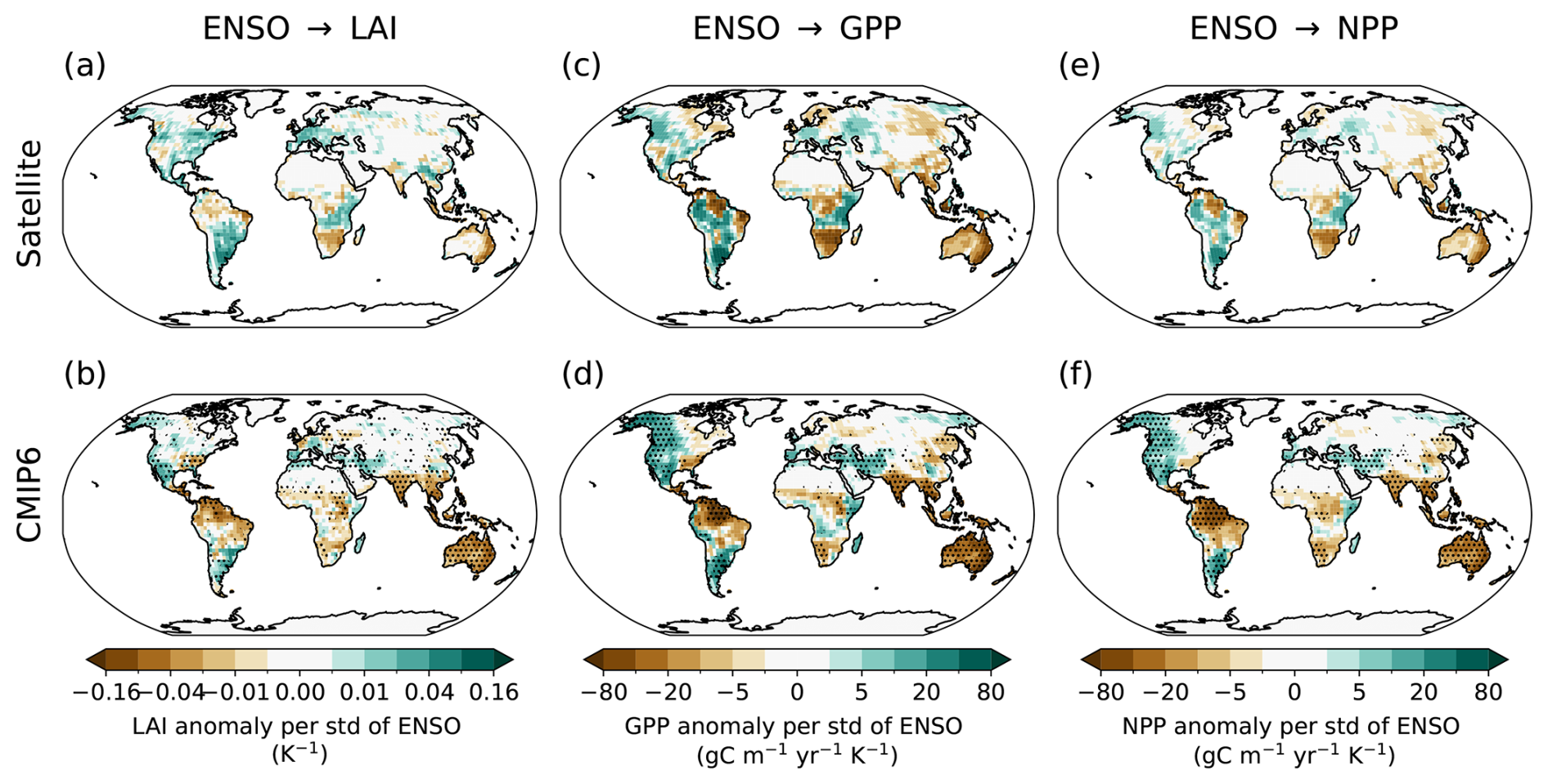
Figure 2 Spatial maps of the regression coefficient of detrended seasonal anomalies in (a, b) LAI, (c, d) GPP, and (e, f) NPP against the Niño3.4 index for the period 1980–2014. The values are normalized by the standard deviation of the Niño3.4 index. (a), (c), (e) show results using observed data: HadISST sea surface temperature for the Niño3.4 index and GLASS satellite observations for LAI, GPP, and NPP. (b), (d), (f) show the MEM results from the CMIP6 historical simulations. Stippling in panels (b), (d), (f) indicates regions where at least 9 out of the 11 CMIP6 models agree on the sign of the change (90 % significance).

3.2 Amplification of ENSO-driven vegetation variability at low frequencies

We utilize 500 years of piControl simulations to examine the long-term variability and causal relationship between ENSO and vegetation structure (LAI). The MEM regression of the seasonal LAI anomaly onto the Niño3.4 index in the piControl runs (Fig. 3a) reveals a coherent spatial pattern highly consistent with the known ENSO teleconnections and the historical simulation results in Fig. 2b. The models agree on the strong teleconnection patterns over a range of different biome types, including the northern and northeastern Amazon, Argentina, India, Australia and the eastern United States. The notable exception is Central Africa (Fig. S1), where considerable inter-model spread likely reflects long-standing CMIP biases in central African climate (Akinsanola et al., 2026).

To test whether vegetation acts as an amplifier of ENSO variability, particularly at low frequencies, we compare the power spectrum of the Niño3.4 index with the spectrum of T_LAI (Eq. 2), which is an index of the covariance of LAI anomalies with Niño3.4 (Fig. 3e). The T_LAI spectrum shows a distinct spectral reddening compared to the Niño3.4 spectrum, characterized by greater power at periods longer than around 5 years and reduced power at interannual timescales.

We quantify the frequency dependence of the total influence (ENSO → LAI) using multi-taper spectral analysis. Strong coherence squared of up to 0.8 is observed at periods of 2–8 years (Fig. 3b). Crucially, the coherence remains statistically significant, with values around 0.4, even at periods past 30 years and up to centennial timescales, confirming a robust relationship across the entire spectrum. A distinct phase lag of around 45° (corresponding to 4–6 months) is observed on interannual to 20-year time scales (Fig. 3c), indicating that LAI changes follow ENSO changes. We can evaluate the reddening at these long timescales using the gain. The gain shows a strong increase (reddening) towards longer periods, consistent with the power spectrum (Fig. 3d–e). At multi-decadal to centennial timescales, the MEM gain is around 1.20–1.25. This signifies that the ENSO-driven vegetation variability is amplified by approximately 20 %–25 % at long timescales compared to the driving ENSO variability at those timescales. This is especially true in a relative sense when compared to the gain of 0.35–0.75 at 2–4 year timescales, which indicates a 25 %–65 % amplitude reduction of the vegetation variability at these timescales.

To identify the geographical drivers of this global signature, we first conducted a gridcell-resolved analysis (Fig. S2), which confirms that the strongest coherence and reddening are concentrated in tropical hotspots like Amazonia and Southeast Asia. By resolving the signal at each pixel, we verify that the global T_LAI pattern reflects real local dynamics rather than an artifact of spatial cancellation between out-of-phase regional anomalies. These findings are supported by targeted regional spectral analysis of the major tropical rainforest regions (Amazon, Congo and Southeast Asia), which dominate global vegetation productivity and are strongly influenced by ENSO (Fig. S3). While the gains from this regional analysis are not directly comparable to the gain in the global T_LAI index in a quantitative sense, the qualitative behavior in the Amazon and Southeast Asia shows pronounced spectral reddening and significant decadal coherence, mirroring the global amplification pattern. In contrast, the Congo region shows no coherence on long timescales, which might be related to low model agreement in this region (Fig. 3a).

However, a key question is whether this low-frequency LAI amplification arises directly from ENSO forcing or if it is instead mediated by the PDO, which is known to be closely related to the low-frequency modulation of ENSO (Fig. S4; Zhang et al., 1997; Newman et al., 2016; Wills et al., 2019). A partial spectral analysis was performed to remove the linear influence of the PDO index on the ENSO → LAI relationship (Fig. 3f–h). When excluding the PDO, the partial coherence remains significant, with values of 0.25 at long periods. The partial gain still shows spectral reddening with a MEM gain of around 1 at long periods compared to a MEM gain of 0.35–0.75 at interannual timescales (2–4 years). These results indicate that the majority of the decadal variability in LAI is directly related to ENSO across interannual to centennial timescales and that there is a direct causal relationship between ENSO and decadal LAI variability. Mediation by the PDO accounts for only a small portion of the effect of ENSO on the LAI variability.

This is supported by a mediation analysis using 10-year low-pass filtered data, which yields a MEM total effect (τ) of ENSO on LAI of 1.01 and a direct effect (τ_Z) of ENSO on LAI excluding the influence of the PDO of 0.88, leaving an indirect effect (αβ) via the PDO of only 0.13. Similarly, we can use gain values for this mediation analysis between ENSO (E), LAI regressed on Niño3.4 index (L) and the PDO (P). The total gain (G_EL) is 1.06 for periods larger than 10 years, the direct gain (G_EL|P) is 0.95 and the indirect gain ($G_{\mathrm{EP}}\cdot G_{\mathrm{PL}|\mathrm{E}}$) is 0.11. The slight numerical discrepancy between the time-domain total effect (1.01) and the frequency-domain total gain (1.06) is expected since it arises from the different order of operations in spectral versus multi-model averaging. Nevertheless, these calculations consistently show that the PDO is only a weak partial mediator (accounting for around 12 % of the signal), and a significant portion (around 88 %) of the observed low-frequency amplification in LAI is due to a direct causal relationship between low-frequency ENSO variability and LAI.

Beyond Pacific climate modes, we evaluate the role of the AMV. Although the AMV shows significant coherence with LAI at multi-decadal periods, it does not produce spectral reddening (Fig. S5). A partial spectral analysis conditioning the ENSO → LAI relationship on the AMV index further showed that the multi-decadal gain and coherence remain unchanged (not shown). These results confirm that the AMV is not the driver of the observed low-frequency amplification and does not confound the ENSO-vegetation pathway, reinforcing that the spectral reddening is a property of the ENSO-LAI system.

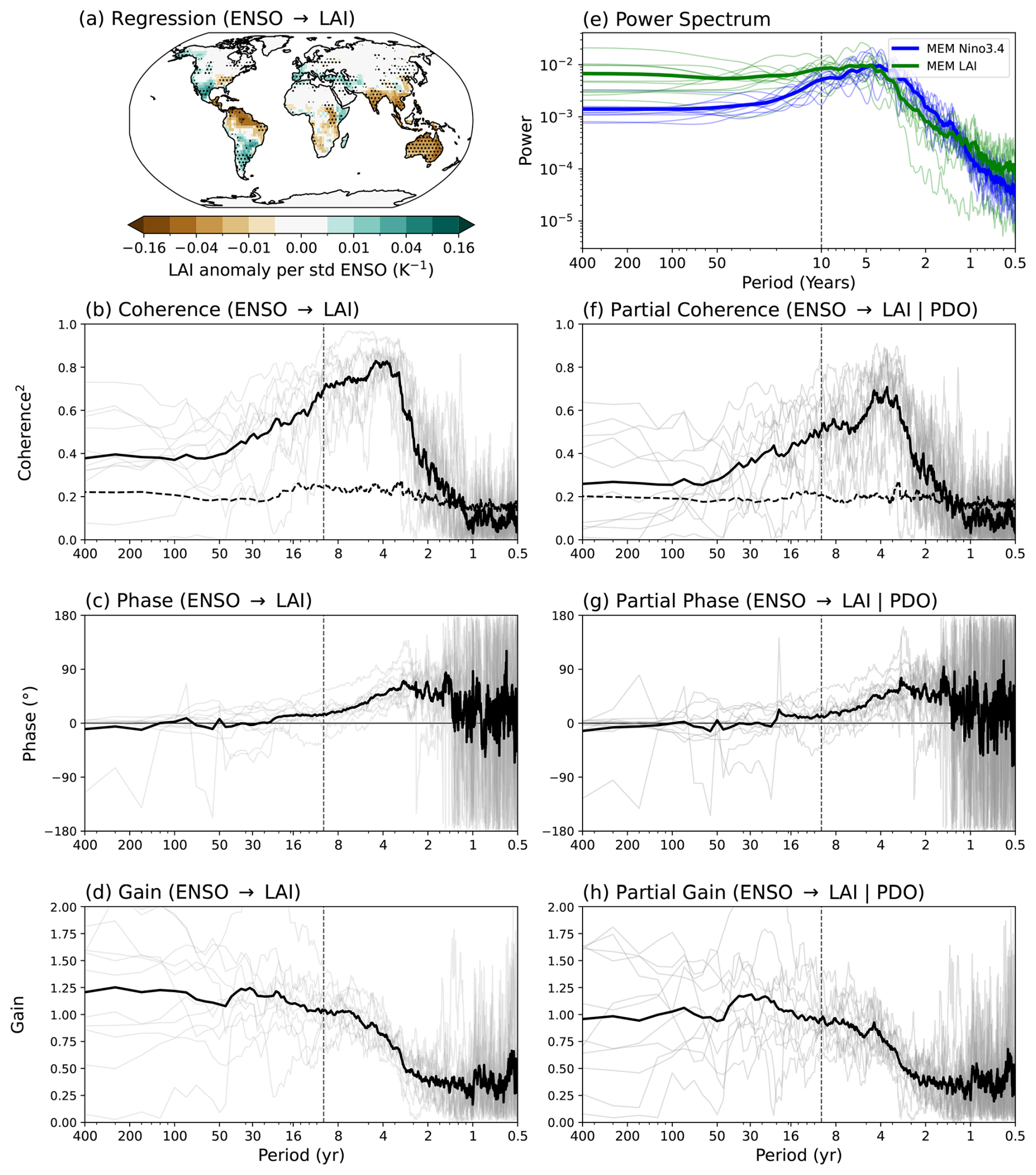
Figure 3 (a) Spatial map of the MEM regression coefficient of seasonal LAI anomalies on the Niño3.4 index, normalized by the standard deviation of the Niño3.4 index. The regression coefficient is calculated for each model based on 500 years of linearly detrended CMIP6 piControl simulations. Stippling indicates agreement on the sign of change by at least 9 of the 11 models (90 % confidence). (b–d) Coherence squared, phase, and gain between the Niño3.4 index and LAI regressed on Niño3.4 in piControl. (e) Power spectrum of the Niño3.4 index (thick blue line for MEM, thin blue lines for individual models) and LAI regressed on Niño3.4 (thick green line for the MEM, thin green lines for individual models) in piControl. (f–h) Partial coherence squared, phase, and gain between the Niño3.4 index and LAI regressed on Niño3.4 in piControl, with the linear influence of the PDO index removed. In panels (b)–(d) and (f)–(h), the thick black line represents the MEM mean, and thin grey lines show individual model results. The black dashed lines in panels (b) and (f) show the critical coherence squared at the 90 % significance level. The dashed vertical lines in panels (b)–(h) mark a period of 10 years.

3.3 Mechanism of low-frequency amplification

To identify the physical mechanism of land-surface memory that leads to spectral reddening from ENSO to LAI, we used partial spectral analysis to sequentially exclude the influence of different climate controls. Vegetation productivity is primarily limited by light availability (energy-limited) or water stress (water-limited) rather than thermal energy, especially in the tropics (Seneviratne et al., 2010). Additionally, temperature can be the dominant control over vegetation growth in mid- and high-latitude biomes (Nemani et al., 2003). Consequently, we focus on four key variables, namely surface downwelling shortwave radiation (RSDS), near-surface soil moisture (MRSOS), deep-layer soil moisture (total soil moisture content MRSO minus MRSOS) and near-surface air temperature (TAS). MRSOS primarily controls soil evaporation and infiltration of precipitation, while MRSO - MRSOS serves as the deep vegetation water source. RSDS reflects fluctuations in surface light availability, acting as the primary energy-related driver for photosynthesis and vegetation growth. If the spectral relationship between ENSO and LAI remains unchanged after excluding one of the specific variables, it suggests that this variable is not a primary mediator of or memory reservoir for the ENSO signal.

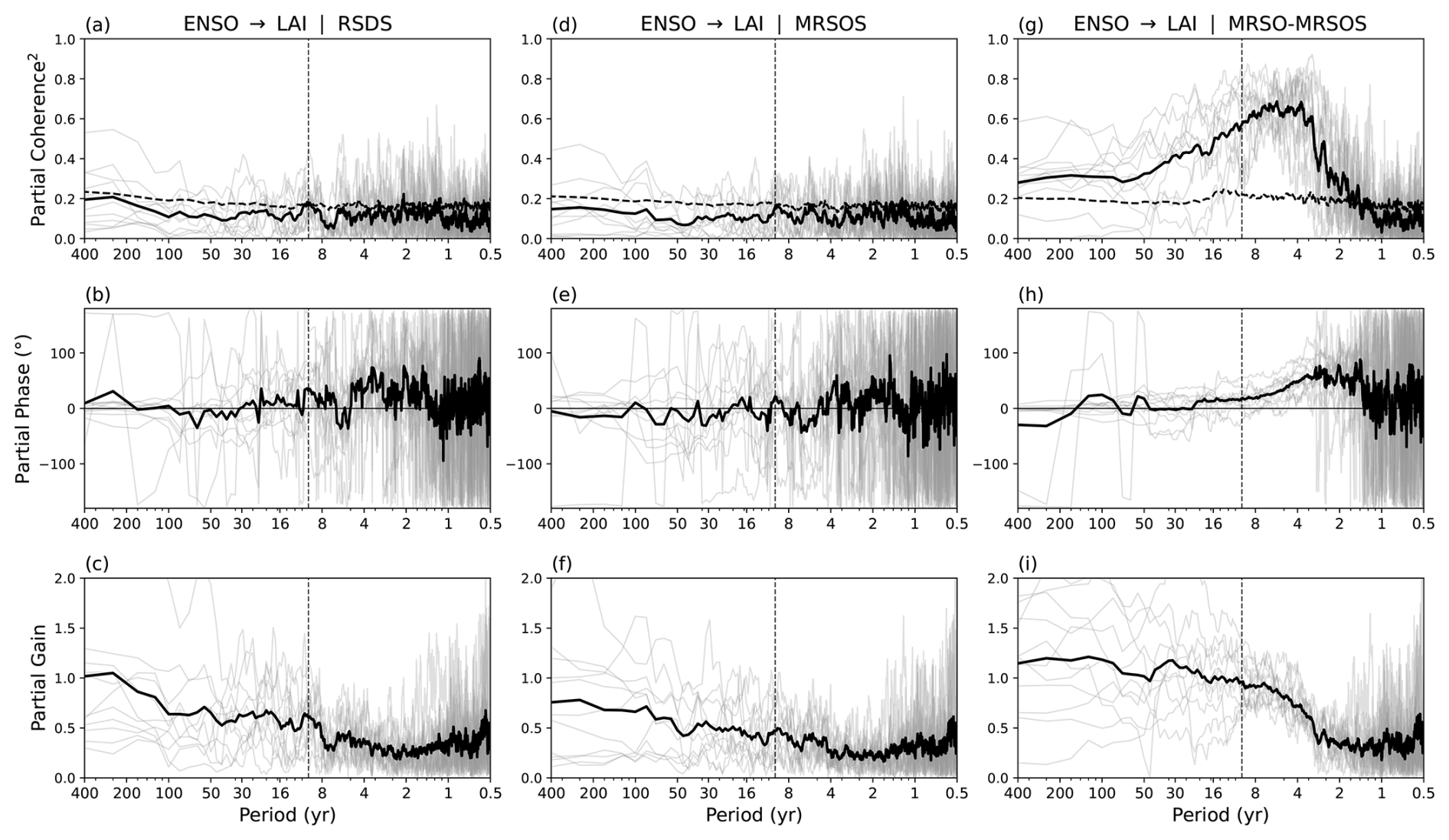
Figure 4 Partial coherence squared, phase, and gain between the seasonal Niño3.4 index and seasonal LAI anomalies regressed on Niño3.4 in piControl, with the linear influence of (a–c) surface downwelling shortwave radiation (RSDS, W m⁻²), (d–f) near-surface soil moisture (MRSOS, kg m⁻²) and (g–i) deep-layer soil moisture (MRSO – MRSOS, kg m⁻²) regressed on Niño3.4 excluded. The thick black line shows the multi-model mean across 11 models, and thin grey lines depict individual model results. The black dashed lines in panels (a), (d), (g) show the critical coherence squared at the 90 % significance level. The dashed vertical lines mark a period of 10 years.

Removing the linear influence of surface downwelling shortwave radiation in the ENSO → LAI pathway causes the partial coherence to drop below the 90 % significance threshold at all timescales (Fig. 4a). Similarly, when conditioning the transfer function on near-surface soil moisture, the coherence falls below the critical limit (Fig. 4d). This is also in line with the coherence breakdown of excluding the influence of net precipitation (precipitation P minus evapotranspiration E) – which determines the input into the soil (Fig. S6). In contrast, excluding near-surface air temperature still gives statistically significant partial coherence across annual to multi-decadal timescales and a persistent spectral reddening. Thus, both radiation and shallow soil moisture could be more critical mediators in the propagation of the ENSO signal to vegetation on a global scale than temperature, although inter-model spread persists. However, the behaviour of the partial gain reveals a key distinction in their roles. When radiation is excluded, the partial gain still exhibits a clear reddening characteristic, with the gain increasing toward lower frequencies and reaching 1.0 at multi-decadal scales (Fig. 4c). Contrarily, excluding near-surface soil moisture significantly flattens this spectral response (Fig. 4f).

These results suggest that while surface downwelling shortwave radiation is a critical driver of vegetation productivity, it cannot provide the memory required for low-frequency amplification in vegetation. Instead, near-surface soil moisture acts as a primary memory source for LAI by integrating precipitation anomalies over time, effectively filtering high-frequency ENSO variations into the sustained, low-frequency anomalies observed in LAI. Interestingly, while the gain from ENSO to near-surface soil moisture is around 1.0 at long periods (not shown), the gain of the total ENSO → LAI pathway reaches approximately 1.20–1.25 (Fig. 2d). This multi-step enhancement suggests that the near-surface soil moisture provides an underlying source of memory, which is subsequently amplified by internal vegetation dynamics at low frequencies.

Unlike the near-surface variables, removing the influence of deep-layer soil moisture does not break the ENSO-LAI link. The partial coherence remains significant at approximately 0.3 at long periods (Fig. 4g). Furthermore, the partial gain (Fig. 4i) maintains a strong reddening signature, reaching a value of 1.2 at multi-decadal timescales, which is nearly identical to the total impact of ENSO on LAI seen previously (Fig. 3). This shows that while the deep layer may hold water for longer periods, the reddening of the ENSO signal is predominantly governed by the interplay between near-surface soil water content and vegetation processes.

3.4 Changes in ecosystem carbon function

Finally, we examine how the vegetation memory signal manifests in two ecosystem carbon fluxes variables, GPP and NPP. The regression pattern of GPP and NPP onto the Niño3.4 index (Fig. 5a, e) is very similar to LAI (Fig. 3a), however showing more model agreement (Figs. S7, S8). The coherence spectrum of GPP and NPP with ENSO is strongest at interannual time scales, but still significant at multi-decadal timescales (Fig. 5b, f). GPP preserves the low-frequency amplification signal, with a spectral gain of around of around 1.20–1.25 at multi-decadal periods and 0.4–0.6 at interannual timescales (Fig. 5d), comparable to the amplification found in LAI. However, while NPP shows spectral reddening, the signal amplification at decadal and longer periods is effectively lost (gain just below 1.0) (Fig. 5h). This means that while the low-frequency ENSO signal is transmitted to NPP, its relative amplitude is not amplified.

The loss of signal amplification in NPP compared to the gain found in GPP is driven by the internal coupling between gross uptake and autotrophic respiration (R_A), where $\text{NPP}=\text{GPP}-R_{\mathrm{A}}$. Coherence analysis between the ENSO-regressed components of GPP and R_A reveals that these fluxes are strongly synchronized at longer timescales (Fig. S9). While the squared coherence is low at sub-annual frequencies, it increases sharply for periods exceeding 2 years, reaching values between 0.8 and 0.9 at decadal and multi-decadal scales. This high coherence indicates that at low frequencies, R_A tracks GPP almost perfectly. Consequently, the amplified low-frequency variability induced by soil moisture and vegetation memory in GPP is largely offset by a nearly identical response in R_A. This internal buffering effectively cancels out the memory-driven amplification, resulting in an NPP gain that remains just below 1.0 despite the strong persistence signal present in the gross carbon exchange. Further studies could investigate whether this reflects a structural model behavior or a real-world biological process. Nonetheless, the result is important as it identifies a potential filtering mechanism that prevents gross productivity memory from translating into net decadal carbon sequestration.

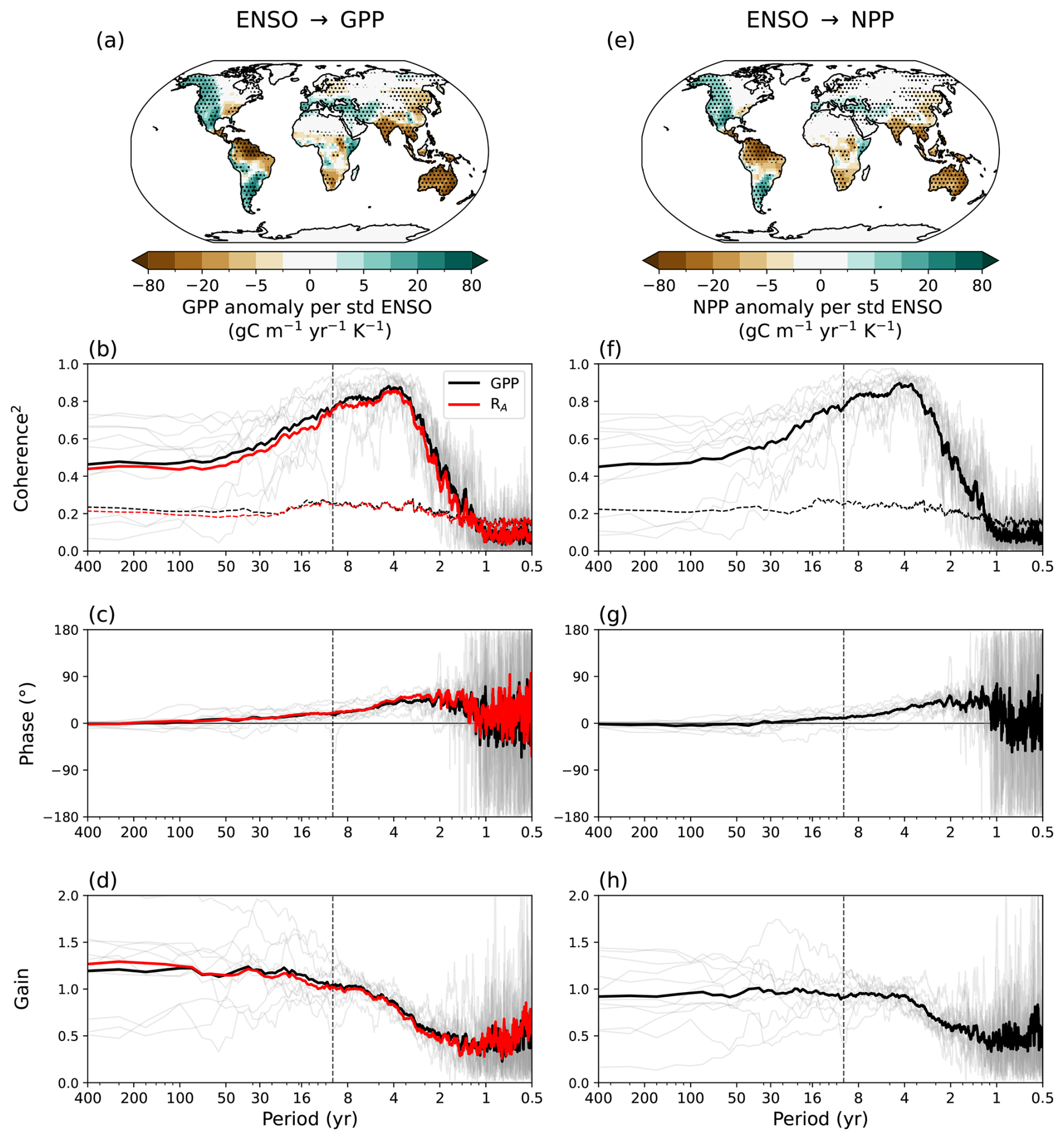
Figure 5 Regression of seasonal anomalies in (a) GPP and (e) NPP on the Niño3.4 index in piControl, normalized by the standard deviation of the Niño3.4 index. The maps show the MEM, and stippling indicates where at least 9 out of 11 models agree on the sign of the change (90 % confidence). (f–h) Coherence squared, phase, and gain between the Niño3.4 index and GPP (black lines) and autotrophic respiration (R_A) (red lines) regressed on Niño3.4. (b–d) Coherence squared, phase, and gain between the Niño3.4 index and NPP. In panels (b)–(d) and (f)–(h), thick lines show the MEM and thin lines individual models (for GPP in b–d). The black and red dashed lines in panels (b) and (f) show the critical coherence squared at the 90 % significance level. The dashed vertical lines in panels (b)–(d), (f)–(h) mark a period of 10 years.

4 Discussion and conclusions

In this study, we analyzed if and how ENSO affects decadal to multi-decadal vegetation variability using multi-centennial piControl simulations from 11 ESMs featuring interactive LAI. Our results provide a frequency-resolved assessment of the memory in the terrestrial system, disentangling the causal pathways through which atmosphere-ocean variability is translated, amplified, and ultimately buffered by the vegetation system.

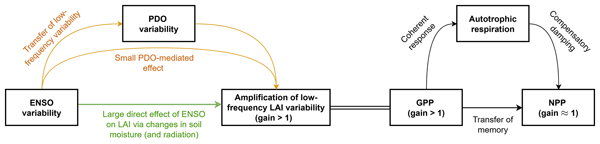
The schematic diagram in Fig. 6 summarizes our findings on the influence of ENSO on terrestrial variability on long timescales. We find an amplification of ENSO-driven LAI variability at low frequencies, leading to spectral reddening and a total gain of around 1.20–1.25 at multi-decadal to centennial periods in the LAI spectrum. This 20 %–25 % amplification of the low-frequency ENSO variability is primarily due to a direct causal link between ENSO and LAI (88 %), while the PDO acts as a weak partial mediator (12 %). The AMV, while showing significant coherence with vegetation, does not contribute to this spectral reddening. The low-frequency memory originates from the ENSO-induced changes in the near-surface soil moisture (and radiation) and is subsequently amplified by internal vegetation dynamics. While this structural memory leads to reddening and amplification of the low-frequency ENSO signal in LAI and GPP, the amplification is suppressed in NPP by a compensatory increase in autotrophic respiration. Overall, these findings show that ecosystems (characterised by LAI and GPP) are an active amplifier of low-frequency atmosphere-ocean variability, but that this memory is ultimately buffered in the net carbon fluxes by changes in autotrophic respiration.

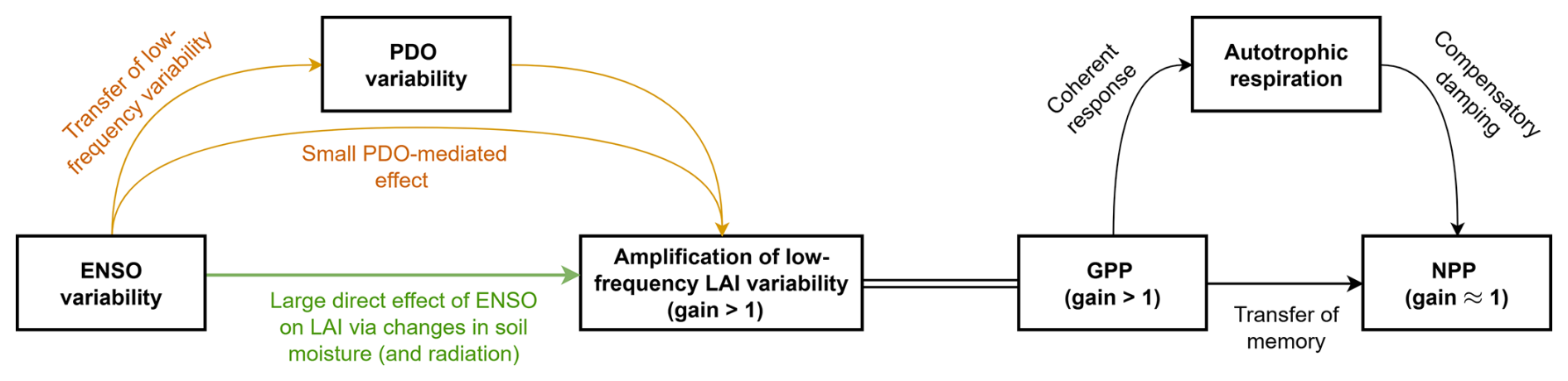
Figure 6 Schematic diagram illustrating the influence of ENSO on LAI variability, both directly and indirectly via changes in the PDO, at decadal and longer timescales. Also shown is the impact on carbon cycle (GPP, autotrophic respiration and NPP).The double line between GPP and LAI indicates that these changes are linked and not unidirectional.

Our core finding – that ENSO-driven vegetation variability is amplified at decadal and longer timescales – extends the established literature on ENSO-vegetation interactions. Previous studies have robustly demonstrated a strong interannual influence of ENSO on ecosystem structure (Buermann et al., 2002; Woodward et al., 2008; Ito, 2011) and its resultant control over interannual fluctuations in the global carbon cycle (Wang et al., 2013; Zhang et al., 2018). Our work extends this understanding by showing that the influence of ENSO variability on vegetation persists into decadal and multi-decadal timescales, particularly in the tropics. This algins with recent single-model analyses showing that decadal ENSO variability influences LAI (Lu et al., 2023) and global land carbon flux variability (Park et al., 2020). Importantly, our multi-model approach adds confidence to these previous single-model results, as the conclusions are less susceptible to specific model parameterizations and demonstrate good agreement with satellite observations during the historical period (Figs. 2, S10). Additionally, we rigorously assessed the mediation of the ENSO influence on vegetation by the PDO, which has been noted to strongly influence decadal-scale carbon flux anomalies (Ito, 2011), although this has not been previously disentangled from the nested influence of ENSO. We robustly quantify that the PDO is only a weak partial mediator between ENSO and LAI, revealing that the majority of the multi-decadal amplification originates from a direct causal link rooted in low-frequency ENSO variability. In contrast, while there is significant multi-decadal LAI variability that is coherent with the AMV, it does not show the reddening that was found for ENSO-driven LAI variability.

We find that the signal reddening and amplification on multi-decadal to centennial timescales are mainly driven by near-surface soil moisture dynamics, which are then further amplified by internal vegetation dynamics. Established literature emphasizes that soil moisture provides a large fraction of the predictability imparted by the land surface on weekly to seasonal timescales (Seneviratne et al., 2010; Rahmati et al., 2024). This predictability is particularly evident during interannual ENSO events, where soil moisture has been identified as the dominant driver of subsequent vegetation productivity changes (Wu et al., 2024). This “soil moisture memory” is widely recognized as a key source for skillful seasonal range forecasts. Our work extends this seasonal focus by providing evidence that by acting as a hydrological buffer, the near-surface soil moisture reservoir filters out high-frequency noise and can sustain LAI anomalies far beyond the seasonal horizon. This behaviour is consistent with the fundamental properties of integrated stochastic processes, where half of the variance in a red-noise spectrum occurs at periods 2π times longer than the physical response time of the system (Roe, 2009). Thus, the multi-decadal variability in the vegetation signal arises as the soil moisture reservoir acts as a physical integrator, shifting variance from interannual ENSO forcing to much longer timescales in LAI and GPP. Furthermore, our finding that the amplification of multi-decadal variability is lost in NPP due to compensatory autotrophic respiration highlights a novel mechanism for the internal buffering of climate memory within the terrestrial carbon cycle.

The advances in our methodology were essential for achieving these detailed, mechanistic insights, offering significant improvements over conventional approaches. While previous efforts relied on standard correlation or regression analysis in the time domain (Ito, 2011; Lu et al., 2023; Park et al., 2020), or simple power spectral density analysis in the frequency domain (Zhang et al., 2018), these methods are fundamentally limited in their ability to robustly quantify causality, disentangle co-varying climate modes, or assess lagged responses across a full spectrum of timescales (Linscheid et al., 2020; Wu et al., 2015). Our methodology overcomes these limitations by using mediation and partial spectral analysis. The use of partial spectral analysis – a method novel to climate science – allows us to cleanly separate relationships in the frequency domain by statistically removing the influence of co-varying signals (e.g., the PDO) from the ENSO to LAI relationship. This addresses the collinearity problem inherent in conventional spectral coherence analysis, enabling a rigorous quantification of the direct causal pathway and leading to our conclusion that the PDO is only a weak partial mediator. Additionally, this frequency-resolved approach enables us to assess temporal patterns beyond simple correlation by using the phase angle to directly determine the causal direction and the precise lead/lag relationship between variables across timescales. This resolves ambiguities inherent to standard mediation analysis, which often requires a priori physical reasoning to rule out bidirectional feedbacks ($X\to Z\to Y$ vs. $X\to Y\to Z$). Finally, our use of the gain metric allows us to quantify not just the relationship, but also the reddening and magnitude of the amplification of the low-frequency signal in LAI. This quantification is then systematically traced through the full causal chain of terrestrial variables, from the structural changes in LAI to the ecosystem carbon changes in GPP and NPP, expanding on previous work that usually focused on only one vegetation-related variable (Ito, 2011; Lu et al., 2023; Park et al., 2020). Overall, the methodological framework used here for frequency-resolved causal diagnosis can be widely applied to other questions in Earth system dynamics.

While our analysis provides valuable insights into how LAI amplifies low-frequency ENSO variability, some key uncertainties and limitations need to be acknowledged. Firstly, an uncertainty in our analysis is the representation of soil moisture memory in models, which remains difficult to validate and likely influences the inter-model spread. While CMIP6 models generally perform well in capturing soil moisture climatology and annual cycles (Qiao et al., 2022), their ability to represent temporal persistence is less certain. Validation is hindered by sparse in situ networks and satellite records that are often restricted to the surface layer or lack the multi-decadal length required to investigate decadal variability. While site-specific studies suggest atmospheric general circulation models can realistically simulate soil moisture memory (Seneviratne et al., 2006), broader global assessments indicate that land surface models may overestimate memory in water-limited regions while underestimating it in energy-limited ones (He et al., 2023). Since soil moisture changes are the foundational driver of the signal reddening we find, these potential biases represent a key uncertainty in the simulated magnitude of the low-frequency vegetation reddening and amplification.

Secondly, while our partial spectral analysis identifies near-surface soil moisture as the primary driver of signal reddening, it is important to recognize that shallow and deep soil layers are physically coupled. In many ESMs, the deeper soil reservoir can influence surface timescales through vertical moisture fluxes. This suggests that the low-frequency memory we attribute to the near-surface may be partially supported by deeper hydrological persistence, a vertical interaction that cannot be fully disentangled using linear spectral methods. Furthermore, because soil moisture, radiation, and precipitation are dynamically interlinked through atmospheric processes (e.g., cloud-precipitation feedbacks), the exclusion of one variable in our spectral analysis inevitably captures a portion of the variance shared by the others, meaning the partial spectral analysis identifies the dominant linear pathway rather than a completely independent physical process.

Thirdly, both the mediation analysis (MacKinnon et al., 2000) and the partial spectral analysis are inherently restricted to capturing linear relationships, thereby excluding potentially significant non-linear effects and interactions.

Finally, while CMIP6 historical simulations show good agreement with the satellite record regarding spatial patterns and spectral signatures (Figs. 1, S8), the models tend to underestimate the intensity of the vegetation response compared to observations. However, satellite-derived benchmarks are themselves subject to uncertainties. For instance, LAI products based on spectral indices are sensitive to cloud cover and atmospheric conditions alongside impacts from orbital drift or sensor changes, which could potentially introduce low-frequency variability (e.g., Wolf et al., 2025; Frankenberg et al., 2021). Furthermore, the use of the piControl simulations, although ideal for isolating internal climate variability, explicitly excludes the influence of anthropogenic forcings, which are known to alter the climate mean state and the ecosystem's sensitivity to ENSO forcing (Le, 2023). Therefore, further work could use future scenario simulations to investigate how ENSO-forced vegetation memory is modified under a warming climate.

Overall, our study contributes to the understanding of coupled ocean-atmosphere-land-vegetation dynamics by providing a frequency-resolved assessment of terrestrial memory. The central finding that the ecosystem acts as an amplifier of low-frequency atmosphere-ocean variability has important implications for decadal climate predictability. Currently, oceanic processes are the primary focus of work aimed at improving decadal forecast skill (Bellucci et al., 2015). However, our results demonstrate that the memory of vegetation, rooted in the near-surface soil moisture, acts as a predictable terrestrial component that can sustain climate anomalies for multi-decadal periods. An increased focus on land-surface initialization – specifically regarding the coupled state of soil moisture and vegetation – within decadal prediction systems could better leverage this terrestrial memory to improve forecasts of regional land surface conditions (e.g., LAI, crop yield potential) at multi-annual lead times, thereby advancing the limited body of previous work that has demonstrated the beneficial impact of realistic vegetation state on prediction skill (Weiss et al., 2012, 2014; Alessandri et al., 2017). Furthermore, the amplification of ENSO's decadal signal into persistent LAI anomalies has significant implications for hydrological risk management. Since persistent LAI anomalies reflect multi-decadal shifts in regional water balance sustained by soil moisture changes, understanding these mechanisms is key for water resource managers when planning for prolonged drought or wet phases that could severely impact agriculture and infrastructure.