Overshoot and (ir)reversibility to 2300 in two CO₂-emissions driven Earth System models

Future climate scenario projections are usually run with prescribed atmospheric CO₂ concentrations. However, by not allowing the carbon cycle to interactively respond to emissions in Earth System models, the role of carbon cycle feedbacks on contributions to differences in climate model projections may be undersampled. Here, we present the main findings of two Earth System Models (MPI-ESM1.2-LR and NorESM2-LM) run with CO₂ emissions to 2300 for three scenarios, two of which are climate overshoot scenarios, that were part of the Coupled Model Intercomparison Project Phase 6 (CMIP6). These experiments serve three important purposes: (i) an increasing focus on emissions driven runs, supplementing scenarios produced for the Coupled Climate-Carbon Cycle (C4MIP) and Carbon Dioxide Removal (CDRMIP) contributions to CMIP6; (ii) a focus on overshoot scenarios; and (iii) an extension of results beyond 2100, the timescales at which some of the most significant differences play out. Of the two models, NorESM2-LM shows more asymmetry in its climate response at the same global mean temperature levels before and after peak warming, particularly in terms of its regional pattern of warming and Atlantic Meridional Overturning Circulation (AMOC) response, with a substantially weakened AMOC persisting for decades after peak warming that takes more than a century to recover. In contrast, MPI-ESM1.2-LR shows reversibility with AMOC strength and regional warming more closely following surface temperature, but with some climate signals such as sea-level rise and ocean deoxygenation essentially irreversible. This diversity in model responses highlights the need for further research with a larger model ensemble that focuses on long-term emissions-driven model runs, particularly for overshoot scenarios, for CMIP7.

1 Introduction

The Coupled Model Intercomparison Project (CMIP), for which CMIP phase 6 (CMIP6) is the most recent completed phase, provides the forum for state-of-the-art Earth System Models (ESMs) to submit results under carefully controlled climate model experimental protocols (Eyring et al., 2016; Taylor et al., 2012). One important component of CMIP is the Scenario Model Intercomparison Project (ScenarioMIP), which evaluates ESM projections into the future and provides insight into how human influences could affect climate due to greenhouse gases, aerosols and land use change (O'Neill et al., 2016; Van Vuuren et al., 2026). In ScenarioMIP, future socioeconomic projections (2015 onwards in CMIP6) are branched from the end of a historical hindcast (1850–2014) under a number of different pathways ranging from very high to very low climate forcing, resulting in a wide range of possible climate change trajectories over the 21st century (Tebaldi et al., 2021). ScenarioMIP experiments provide our best estimates of future climates resulting from these trajectories and are invaluable for informing climate impact models (Rosenzweig et al., 2017). The climate impact models describe how climate change could affect human and natural systems such as crop productivity, biodiversity and human health (Wells et al., 2026a).

In CMIP6, future climate projections are based upon the Shared Socioeconomic Pathway/Representative Concentration Pathway (SSP-RCP) matrix (O'Neill et al., 2016). Scenarios run in ESMs are of the form SSPn-x, where $n=\mathrm{1},\mathrm{\dots },\mathrm{5}$ describes a specific socioeconomic storyline and x describes the approximate radiative forcing level (as a proxy for warming level and climate change mitigation effort) in the year 2100 in W m⁻² (Gidden et al., 2019). A total of eight SSP-RCP combinations were chosen for running in ESMs for CMIP6, spanning radiative forcing targets from 1.9 to 8.5 W m⁻² in 2100. For reference, present-day radiative forcing levels are around 3 W m⁻² (Forster et al., 2025).

For each SSP-RCP, an emissions pathway is produced by an integrated assessment model (IAM). The IAM uses inputs of population, GDP, education and urbanization, and produces greenhouse gas (GHG) and short-lived climate forcer (SLCF) emissions projections as an output. IAMs are internally consistent representations of the economy, energy and land use system, which typically find cost- or welfare-optimising solutions from the input boundary conditions subject to technological, socioeconomic, physical, and climatic constraints (here, the 2100 radiative forcing level). Typically, as the radiative forcing constraint tightens (decreasing W m⁻² target value), climate abatement costs increase and facilitate the requirement for negative emissions technologies. The ease of meeting particular radiative forcing levels depends on the SSP storyline which has different levels of challenges to mitigation and adaptation, with some RCP levels either above the no-mitigation baseline or not technologically feasible within given socioeconomic constraints in some SSPs (Rogelj et al., 2018).

IAMs produce time-varying emissions of CO₂ and other forcers, but future climate experiments in ScenarioMIP and its earlier predecessors were driven by concentrations of CO₂ and other GHGs. The concentrations in each SSP-RCP were calculated using a simple climate model, MAGICC, which uses a carbon cycle box model that is calibrated on full-complexity carbon cycle and Earth system models (Meinshausen et al., 2011, 2017, 2020). However, in addition to supplying the concentration-driven ScenarioMIP experiments, around a dozen ESMs in CMIP6 were set up to run with prescribed emissions of CO₂ (Lee et al., 2021). Performing emissions-driven runs allows us to sample an additional dimension of uncertainty, namely the strengths of climate-carbon-cycle feedbacks that define the atmospheric airborne fraction and land and oceanic uptake of CO₂ emissions (Friedlingstein et al., 2006). Since humans emit greenhouse gases rather than having direct control over atmospheric concentrations, an emissions-driven experimental design is also more appropriate for determining the levels of residual or negative emissions required to stabilize and reverse anthropogenic climate change (MacDougall et al., 2020), as well as more clearly linking model responses to human efforts to reduce emissions.

Under CMIP6, a handful of CO₂ emissions-driven simulations were performed under the SSP5-8.5 (fossil-fuel driven, very high emissions) and SSP5-3.4-over (following SSP5-8.5 until 2040, with rapid emissions reductions after 2040 and high levels of net negative CO₂ emissions in the second half of the 21st century) under the Coupled Climate–Carbon Cycle Model Intercomparison Project (C4MIP) and Carbon Dioxide Removal Model Intercomparison Project (CDRMIP) components of CMIP6 respectively (Jones et al., 2016; Keller et al., 2018; O'Neill et al., 2016). While scientifically interesting and useful for impact studies (Sarofim et al., 2024), SSP5-8.5 has been criticised for being an unrealistically high emissions scenario (Hausfather and Peters, 2020), which would require a global reversal of policy and shift back to fossil fuels (Hausfather, 2025) leading to warming projections at the end of the century in the region of 5 °C above pre-industrial (Tebaldi et al., 2021). The ensuing climate damages from such a strong warming scenario would severely impact the economy and slow growth and ensuing emissions (Woodard et al., 2019; Schoenberg et al., 2025), making this scenario an unlikely reality. It has been argued that SSP5-3.4-over is also unrealistic given its abrupt turnaround and reliance on high levels of carbon dioxide removal (Schleussner et al., 2024).

The CMIP6 protocol allows for (concentration-driven) scenario projections to be extended beyond 2100 to 2300, but only a few models performed the extensions (Lee et al., 2021). Beyond 2100, climate responses in models can differ substantially, and slow feedbacks and irreversibilities only become apparent on these timescales (Solomon et al., 2009). Furthermore, 2100 is now less than one human lifetime away (Lyon et al., 2022). Further studies using emissions-driven experiments have been undertaken in recent years, but realistic experiments may usually only be run to 2100 (Murphy et al., 2014; Fyfe et al., 2021), with longer term experiments tending to be more idealized scenarios such as immediate zeroing of CO₂ emissions (Sigmond et al., 2020; King et al., 2024). For the reasons above, there is interest in running more plausible and policy-relevant climate scenarios in CO₂ emissions-driven ESMs, and these are intended to play a more important role in the upcoming CMIP7 phase beyond 2100 (Sanderson et al., 2024; Van Vuuren et al., 2026).

These considerations motivate two research questions:

1. how do overshoot and negative emissions manifest in responses in the global carbon cycle?

2. to what extent are responses within the Earth system irreversible after a climate overshoot?

Fully answering both research questions requires a longer time horizon than 2100 to analyse long-term impacts and reversibility, and an ensemble of simulations to account for internal variability in climate and the carbon cycle. Pfleiderer et al. (2024) explored the responses in regional and extreme climate in overshoot scenarios in a multi-model ensemble context to 2100, and found that there was asymmetry in the responses before and after peak warming. Roldán-Gómez et al. (2025a, b) used extended simulations to 2300 available for four models in ssp534-over, for which the longer term AMOC response exhibits a wide variety of behaviours. Koven et al. (2022) evaluated the global temperature, carbon stock and AMOC behaviour in five ESMs and one ESM of intermediate complexity in SSP5-3.4-over and SSP5-8.5 simulations run to 2300, noting substantial differences in AMOC and carbon uptake. However, these studies used simulations with prescribed concentrations, limiting the insight that changing emissions has on the carbon cycle and global climate.

In this paper, we run two ESMs under SSP1-1.9 (very low emissions, consistent with the 1.5 °C Paris Agreement goal), SSP2-4.5 (moderate emissions, most closely aligned to current policies with a projected warming in 2100 of around 2.5–3 °C), as well as adding additional simulations of SSP5-3.4-over (included under the Carbon Dioxide Removal Model Intercomparison Project (CDRMIP; Keller et al., 2018)) to 2300. Therefore, we fill in the emissions-driven scenario space at the low and moderate levels compared to the availability of CMIP6 simulations. These runs are primed to study this question because emission-driven ESM simulations give a more detailed representation of the carbon cycle compared to concentration-driven simulations, which take their prescribed concentration pathways from simpler climate models or emulators (Sanderson et al., 2024). While emissions-driven experiments for net-zero and net negative pathways do exist, they have tended to be run with idealized, CO₂-only trajectories (Schwinger et al., 2022b; Tokarska and Zickfeld, 2015). Running emissions-driven scenarios for a longer timeframe allows us to determine the carbon cycle, reversibility, and climate response to climate overshoot under negative emissions. These topics will become increasingly important as the 1.5 and 2 °C warming thresholds are approached in the absence of robust mitigation (Schleussner et al., 2024).

2 Experimental design

We use two emissions-driven ESMs: the Norwegian Earth System Model (NorESM2-LM; Seland et al., 2020; Tjiputra et al., 2020) and the Max-Planck-Institute Earth System Model (MPI-ESM1.2-LR; Mauritsen et al., 2019). These two ESMs are two of the best performing models with respect to reproducing observed atmospheric CO₂ concentrations in the historical period (Fig. 1). Given their good correspondence to historical concentrations, the MPI-ESM1.2-LR and NorESM2-LM models are appropriate for the analysis of future CO₂ emissions-driven simulations.

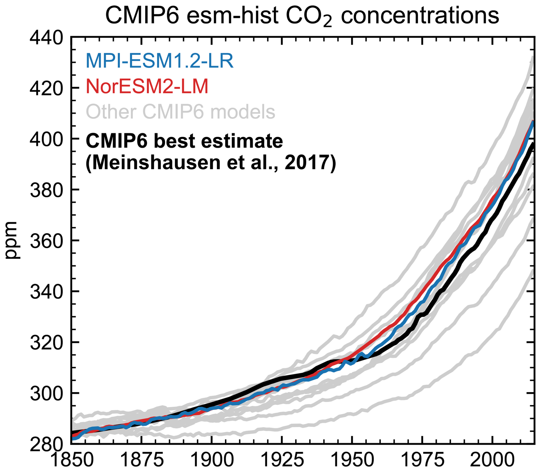
Figure 1 Atmospheric CO₂ concentrations reported from the emissions-driven historical simulations (esm-hist) from the C4MIP contribution to CMIP6 (Jones et al., 2016). NorESM2-LM (red), MPI-ESM1.2-LR (blue), and the other 11 CMIP6 models (light grey) are compared to the best estimate concentration time series that was used to run concentration-driven scenarios (Meinshausen et al., 2017, black).

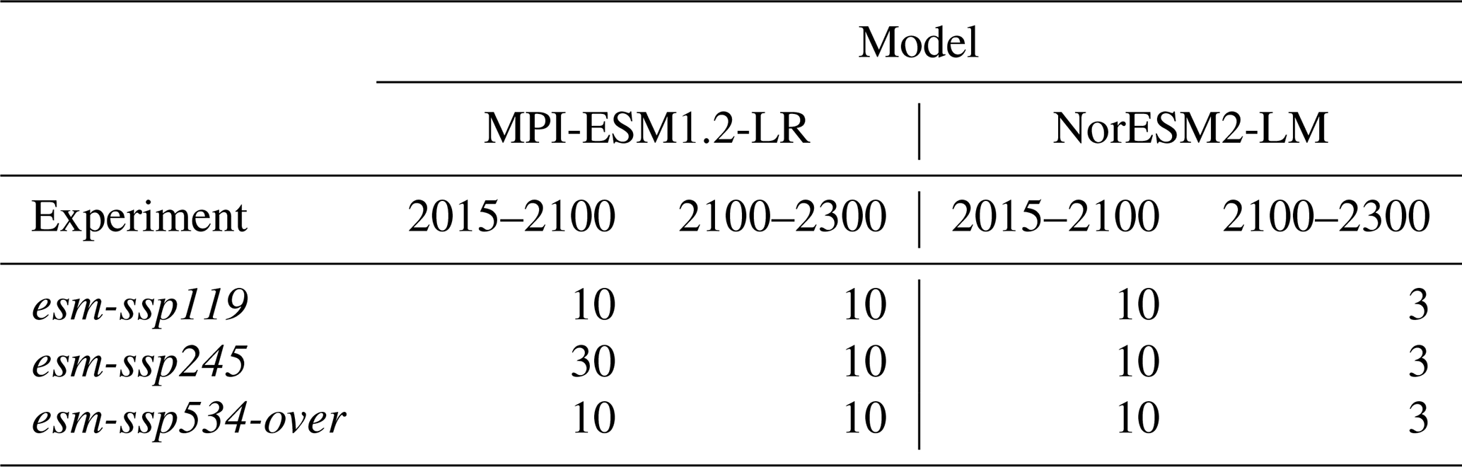
The future scenarios are run from 2015 to 2300 and are labelled esm-ssp119, esm-ssp245, and esm-ssp534-over for SSP1-1.9, SSP2-4.5 and SSP5-3.4-over respectively. They are branched from CO₂ emissions-driven historical simulations (1850–2014) known as esm-hist. In this paper, we follow the CMIP convention of labelling scenarios, which disallows the period “.” symbol (so the radiative forcing target is multiplied by 10) and removes the dash “-” between the SSP and RCP part of the scenario name. For additional distinction we italicize the CMIP6 name, hence ssp119 = SSP1-1.9. Furthermore, we again follow the CMIP6 convention of labelling CO₂ emissions-driven scenarios as run in “Earth system model” mode, so our emissions-driven scenarios are prepended with “esm-”, e.g. esm-ssp119. Table 1 shows the ESM simulations performed within the project along with the number of ensemble members available for each model.

Table 1 Number of ensemble members of the emission-driven simulations with the two ESMs used in this study, with the time periods supported by each ensemble size.

The ESMs are forced with the CO₂ emission pathways used in the SSP scenarios, extended after the year 2100 as described in Meinshausen et al. (2020). Figure 2 shows the prescribed evolution of fossil fuel and industrial CO₂ emissions in both models. The original CMIP6 extension protocol mandates that positive levels of CO₂ emissions in 2100 are extended linearly to zero between 2100–2250, while negative emissions in 2100 are held constant for 40 years. After that, CO₂ emissions linearly approach zero, which takes 30 years in esm-ssp534-over and 45 years in esm-ssp119. MPI-ESM1.2-LR implemented this protocol exactly, while NorESM2-LM implemented it differently such that negative emissions in esm-ssp119 start to linearly approach zero from 2100 with no phase of constant negative emissions. CO₂ emissions from land use change are part of the terrestrial carbon cycle and are determined interactively by each ESMs. Land use transitions follow that of the underlying CMIP6 scenario, and no further land use transitions occur after 2100. Harvest rates are also held constant at 2100 levels for the post-2100 extensions. Non-CO₂ GHGs are prescribed using pre-calculated concentration time series from Meinshausen et al. (2020).

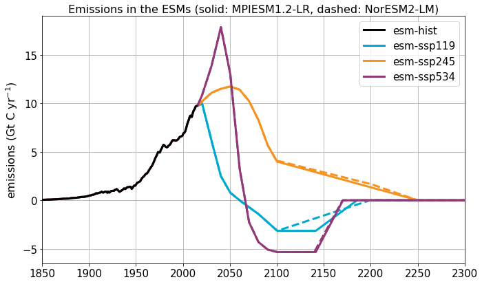
Figure 2 Evolution of total CO₂ emissions for the esm-hist, esm-ssp119, esm-ssp245 and esm-ssp534-over scenarios in MPI-ESM1.2-LR (solid) and NorESM2-LM (dashed).

In MPI-ESM1.2-LR, aerosols are prescribed using concentrations, in the form of the aerosol optical depth (AOD) from the MACv2-SP simulator (Stevens et al., 2017). AOD is reduced linearly to zero between 2100 and 2250 if aerosol emissions are mostly associated with industrial processes in a specific region. In contrast to that, they are held constant after 2100 if they are mostly associated with biomass burning. This matches the information given to the land modules of the ESMs. In NorESM2-LM, aerosols are emissions-driven, and emissions of black carbon, organic carbon and sulfur follow the extension pathways of Meinshausen et al. (2020).

3 Results

3.1 Global surface temperature and CO₂ concentration

Figure 3 shows how MPI-ESM1.2-LR and NorESM2-LM simulate the evolution of the global-mean 2 m surface air temperature (GSAT) anomaly compared to the 1850–1900 reference period (top row) and the atmospheric CO₂ concentration (bottom row) for esm-ssp119, esm-ssp245, and esm-ssp534-over. MPI-ESM1.2-LR shows an earlier warming over the historical period than NorESM2-LM. NorESM2-LM has a lower peak warming than MPI-ESM1.2-LR in the two overshoot esm-ssp119 and esm-ssp534-over scenarios, and a lower 2100 warming in all three scenarios, but is equal to or above the temperature anomaly of MPI-ESM1.2-LR in 2300 in all three.

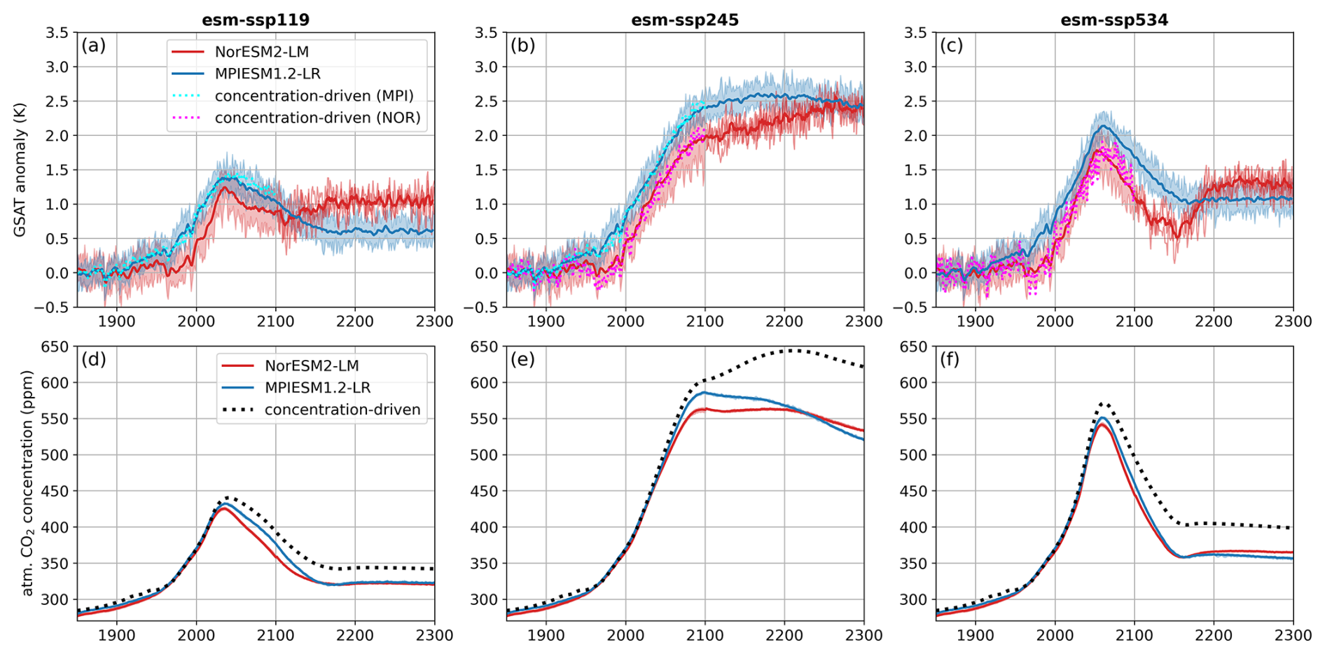
Figure 3 The evolution of the global mean temperature anomaly (a–c) and the atmospheric CO₂ concentration (d–f) in NorESM2-LM and MPI-ESM1.2-LR for esm-ssp119 (a, d), esm-ssp245 (b, e), and esm-ssp534-over (c, f). Shown are the ensemble mean, as well as the full range spanned by the ensemble members for the emissions-driven simulations. Where available, the parallel data from the concentration-driven simulations is given with dotted lines (temperature for ssp119 in MPI-ESM1.2-LR and for ssp534-over in NorESM2-LM, and CO₂ concentration time series from Meinshausen et al. (2020) for all three scenarios).

The difference in future projected behaviour is driven by different responses in the models to zero and net negative CO₂ emissions phases. Both models have (150-year Gregory) equilibrium climate sensitivities (3.00 °C MPI-ESM1.2-LR; 2.54 °C NorESM2-LM) and transient climate responses (1.84 °C MPI-ESM1.2-LR; 1.48 °C NorESM2-LM) that are not vastly different from each other (Smith et al., 2021), therefore likely not accounting for the differences in model projections, particularly in the long term. In esm-ssp119 and esm-ssp534-over, NorESM2-LM shows an increasing temperature in the 22nd century following a temperature minimum before a stabilization in the 23rd century that is qualitatively different from the long-term stabilization in MPI-ESM1.2-LR. In the esm-ssp245 scenario, NorESM2-LM continues to warm in the long term whereas MPI-ESM1.2-LR exhibits a peak temperature in the late 22nd century followed by a decline.

Differences in GSAT evolution in NorESM2-LM compared to MPI-ESM1.2-LR can be explained by differences in ocean circulation. Generally, a slow warming in NorESM2-LM is due to the delayed Southern Ocean response to climate forcing, whereby heat is transported downwards initially and re-emerges towards the surface later in the simulation (Gjermundsen et al., 2021); note also that this behaviour is also observed in an Earth system model of intermediate complexity (Frenger et al., 2025). While a very different forcing profile, similar results are noted comparing 150-year and 500-year simulations of the abrupt-4xCO2 idealized simulation in NorESM2-LM (Wells et al., 2026b). It is known that NorESM2-LM has a low climate sensitivity over timescales of 150 years, roughly that of the CMIP6 historical period, but a much higher climate sensitivity when evaluated over 500 years (Gjermundsen et al., 2021; Seland et al., 2020), caused by changes in the shortwave cloud feedback strength that are driven by the Southern Ocean surface temperature. A second factor, explaining the temperature minima after the GSAT peak in the NorESM2-LM esm-ssp119 and esm-ssp534-over simulations is the decline and recovery of the Atlantic meridional overturning circulation (AMOC), which is much more pronounced in NorESM2-LM compared to MPI-ESM1.2-LR (Sect. 3.4). In overshoot scenarios, where atmospheric CO₂ is reduced at the same time as the northward heat transport is diminished, a strong northern high-latitude cooling followed by a warming has been described in NorESM2-LM (Schwinger et al., 2022a, b). These differing long-term responses highlight the benefits of running climate scenarios beyond 2100.

As MPI-ESM1.2-LR ran ssp119 and ssp245 and NorESM2-LM ran ssp245 and ssp534-over as part of CMIP6, both concentration-driven and only to 2100, it is possible to see the effects of the inclusion of the carbon cycle on the global mean temperature by comparing parallel emissions- and concentration-driven simulations. In all of the four cases, the 21st century warming projections are slightly lower for the emissions-driven runs than for the concentration-driven runs, because of lower atmospheric CO₂ concentrations resulting in a lower radiative forcing in the emissions-driven runs. This is because the ocean and land carbon sinks in these ESMs are stronger than in the MAGICC simple climate model used to derive the prescribed concentration time series. The differences are smallest between esm-ssp245 and ssp245, where the concentrations deviate noticeably only after mid-century, and larger for the overshoot scenarios where the emissions-driven and concentration-driven runs diverge earlier. In the two overshoot scenarios, the divergence in atmospheric concentrations begins around the time of peak emissions, highlighting the need for a better calibration of simple climate models beyond 2100 and under overshoot conditions. More generally the need for better understanding of the behaviour of the carbon cycle in an at-yet unrealized post-peak world is necessary.

As the concentration-driven simulations end in the year 2100, it can be speculated that the increasing differences in atmospheric CO₂ would also cause substantial deviations in the global mean temperature in the 22nd and 23rd centuries between emissions- and concentration-driven scenarios. The post-2100 trajectory of concentrations in esm-ssp245, in which MPI-ESM1.2-LR has concentrations declining more rapidly than NorESM2-LM following their peak, would likely result in lower GSAT projections in both models compared to their ssp245 counterparts.

By analysing global mean temperature anomaly as a function of cumulative CO₂ emissions (Fig. 4), we can first note that both ESMs follow the approximately linear relationship between cumulative CO₂ emissions and temperature (Allen et al., 2009; Matthews et al., 2009) between the start of the simulation and net zero CO₂ emissions in both esm-ssp119 and esm-ssp534-over (light coloured points in Fig. 4). Both models imply a negative zero emissions commitment (ZEC) on the decadal timescale, evidenced by the cumulative emissions-temperature plot curving below the positive emissions phase in the first few decades after net zero (Koven et al., 2023), highlighted by the darker points in Fig. 4. The decadal timescale negative ZEC in these two models is also reported in idealized CO₂-only experiments to zero emissions in MacDougall et al. (2020), though it should be highlighted that the comparison is not directly applicable as our scenarios go to net negative carbon emissions and include non-CO₂ forcers. However in NorESM2-LM the ZEC after 100 years reverses sign and becomes positive, and warming is also reported during net negative carbon emissions phases in idealised overshoot scenarios in this model (Schwinger et al., 2022b). In esm-ssp119 (Fig. 4a), GSAT reaches a minimum around 2110, after which warming increases despite still being in a phase of net negative CO₂ emissions, until stabilization around 2160. NorESM2-LM's response in esm-ssp534-over is more extreme (Fig. 4b), showing a rapid warming of around 0.8 °C in the second half of the 22nd century. This is the period shortly after the scenario transitions from a constant negative emissions of −5.2 Gt C yr⁻¹ in 2140 to zero in 2170.

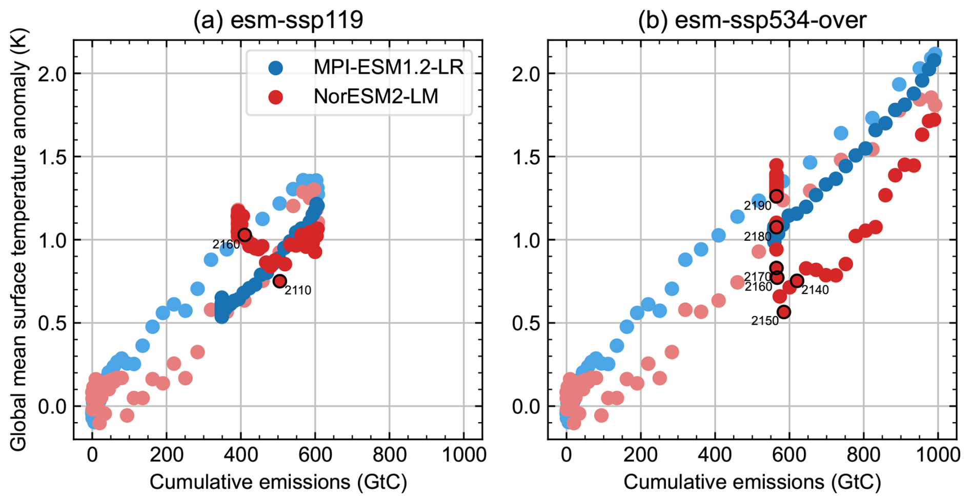
Figure 4 Global-mean surface temperature anomaly as a function of cumulative emissions in MPI-ESM1.2-LR (blue) and NorESM2-LM (red). Light-coloured points show the phase before net zero emissions, dark-coloured points after net zero emissions. Scatter points represent 5-year means of ensemble means. Selected times of five-year means are marked for NorESM2-LM.

3.2 Carbon cycle response

Figure 5 shows how anthropogenic carbon is distributed between the three main reservoirs on Earth (atmosphere, ocean, land) in NorESM2-LM and MPI-ESM1.2-LR. Generally, both ESMs show a very similar distribution of carbon, in which initially most of the carbon from anthropogenic emissions remains in the atmosphere, with the ocean becoming the dominant sink of carbon in the long term. During the historical period, the land-use driven loss of carbon from the land reservoir is slightly stronger in NorESM2-LM than in MPI-ESM1.2-LR, but this is compensated by a slightly larger oceanic uptake of carbon, so that the atmospheric carbon reservoir remains approximately the same in both models. During the 21st century, the total land carbon uptake in NorESM2-LM catches up with that in MPI-ESM1.2-LR, and by the end of the century, more carbon is stored in the biosphere in NorESM2-LM than in MPI-ESM1.2-LR in all scenarios. At the same time, the total ocean carbon uptake is larger in NorESM2-LM, which explains the apparent reduction in the atmospheric CO₂ concentration compared to MPI-ESM1.2-LR. After the year 2100, NorESM2-LM is forced with less negative emissions in esm-ssp119 and has an apparent closure error in the carbon balance in esm-ssp534-over, which is an identified issue in many CMIP6 carbon-cycle enabled models (Tang et al., 2025). Both cases can be interpreted as forcing NorESM2-LM with less negative CO₂ emissions after 2100, and in both cases this leads to roughly 40 GtC that is added to the Earth system in NorESM2-LM compared to MPI-ESM1.2-LR at the end of the simulation, which complicates the comparison of the two models. Nevertheless, when accounting for this complication, some differences in the long-term carbon cycle response can still be analysed. First, the initially stronger land carbon sink in NorESM2-LM declines after 2100, leading to a cumulative land carbon sink that is smaller in NorESM2-LM than in MPI-ESM1.2-LR in the scenarios esm-ssp245 and esm-ssp534-over. However, this is not the case in esm-ssp119, where the land carbon sink of NorESM2-LM still exceeds that of MPI-ESM1.2-LR by around 20 GtC at the end of the simulation, which is potentially a consequence of the less negative emissions in this simulation in NorESM2-LM. The cumulative land carbon sink in NorESM2-LM shows an approximately similar behaviour in the esm-ssp119 and esm-ssp534-over scenarios, whereas in MPI-ESM1.2-LR it is consistently weaker in esm-ssp119 than in esm-ssp534-over, hence the difference comes mainly from a larger scenario-dependence in MPI-ESM1.2-LR. Many processes could be the cause of this, and a deeper analysis would be necessary for a comprehensive answer. One potential candidate is the smaller difference in global mean temperatures between the two scenarios, when using NorESM2-LM. Second, the generally larger cumulative ocean carbon uptake in NorESM2-LM is unlikely to be solely explainable by the (effectively) higher CO₂ emissions in NorESM2-LM, which could also have a range of possible explanations and require a deeper analysis for better understanding.

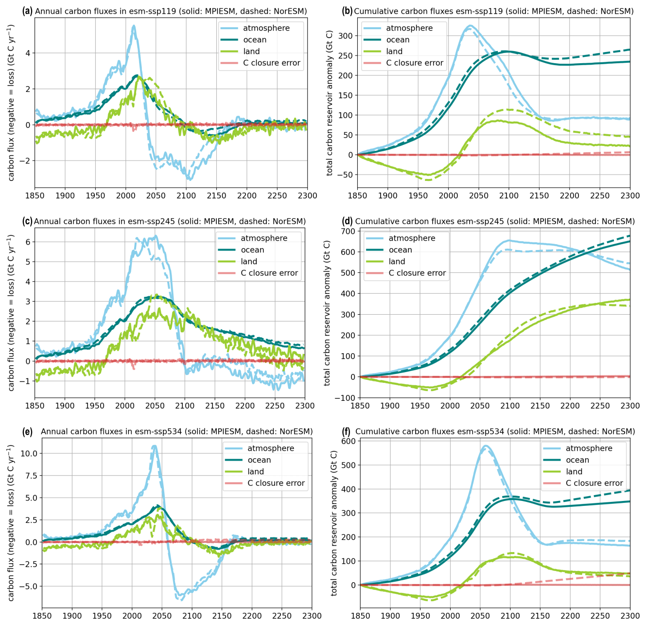
Figure 5 The distribution of (a, c, e) annual and (b, d, f) cumulative carbon stocks between atmosphere, ocean and land in the three scenarios esm-ssp119 (a, b), esm-ssp245 (c, d), and esm-ssp534-over (e, f). The ensemble mean data are shown as a 5-year running mean to reduce interannual variability. Solid lines refer to MPI-ESM1.2-LR and dashed lines refer to NorESM2-LM. The apparent closure error in NorESM2-LM in esm-ssp534-over can be interpreted as less negative emissions of CO₂ after 2100, having a similar effect as the less negative emissions prescribed in esm-ssp119 in NorESM2-LM (Fig. 2).

In all scenarios, the higher atmospheric CO₂ concentrations between 2050–2150 in MPI-ESM1.2-LR can be explained by the weaker ocean and land sink strengths. The weaker land sink is particularly pronounced in esm-ssp119, and persists until the end of the simulation (Fig. 5b). In both overshoot scenarios, the land and ocean both transition from a net sink to a net source of carbon around 2100 (Fig. 5a and e). While the ocean returns to being a carbon sink after 2150, the land continues to emit carbon back to the atmosphere. The annual fluxes are small so these effects are best interpreted from the changes in stocks (Fig. 5b and f).

3.3 Global signs of hysteresis and irreversibility

Next, we specifically look for signs of hysteresis and irreversibility in the climate and carbon cycles in the overshoot scenarios. We define hysteresis to mean a dependence on history (path-dependence) and irreversibility to mean an inability to return to a previous state.

The Atlantic Meridional Overturning Circulation (AMOC) is often considered to be one of the major tipping elements in the Earth system (Rahmstorf, 1995; Wunderling et al., 2024). Figure 6 shows that there is a major difference in the evolution of the AMOC between NorESM2-LM and MPI-ESM1.2-LR, with MPI-ESM1.2-LR showing much smaller variations over time. While both models show a reduction in the AMOC index during the warming period, NorESM2-LM also shows an initial increase during the 20th century, and a much stronger reduction during the first half of the 21st century. In contrast to NorESM2-LM, MPI-ESM1.2-LR exhibits a near-linear relationship between global warming and AMOC reduction, which also holds during the cooling periods in the overshoot scenarios. However, this AMOC weakening only starts at around 0.5 °C above pre-industrial temperatures. There are also small deviations from the linear relationship in MPI-ESM1.2-LR. In the initially rapidly warming scenario esm-ssp534-over, the lowest AMOC indices are reached only after the peak warming period, when the climate has already started to cool. Furthermore, in esm-ssp245, there is some AMOC recovery in the late stages of the simulation, already before the warmest year is reached. Both of these effects are also present and even stronger in NorESM2-LM, which does not exhibit the same linear relationship between AMOC and temperature that MPI-ESM1.2-LR shows. In addition, NorESM2-LM also shows a much faster AMOC recovery than MPI-ESM1.2-LR and even an overshoot of the AMOC strength. This is concurrent with the second warming period unique to NorESM2-LM (Schwinger et al., 2022a), and may be implicated in the rapid warming in the late 22nd century in this model. The AMOC reduction causes an increased ocean heat uptake, which happens at the same time that atmospheric CO₂ is reduced by the negative emissions. When AMOC picks up again at that time atmospheric CO₂ is approximately stabilized, ocean heat uptake decreases such that SAT increases again. It should be noted that a diversity of Atlantic Ocean heat transport (closely related to AMOC) profiles is seen in other models run with CO₂ concentrations to 2300 in ssp534-over, including a persistent weakened state from the middle of the 21st century, and a continued weakening post-overshoot akin to an AMOC collapse (Roldán-Gómez et al., 2025b). This highlights the importance of running simulations longer than to 2100.

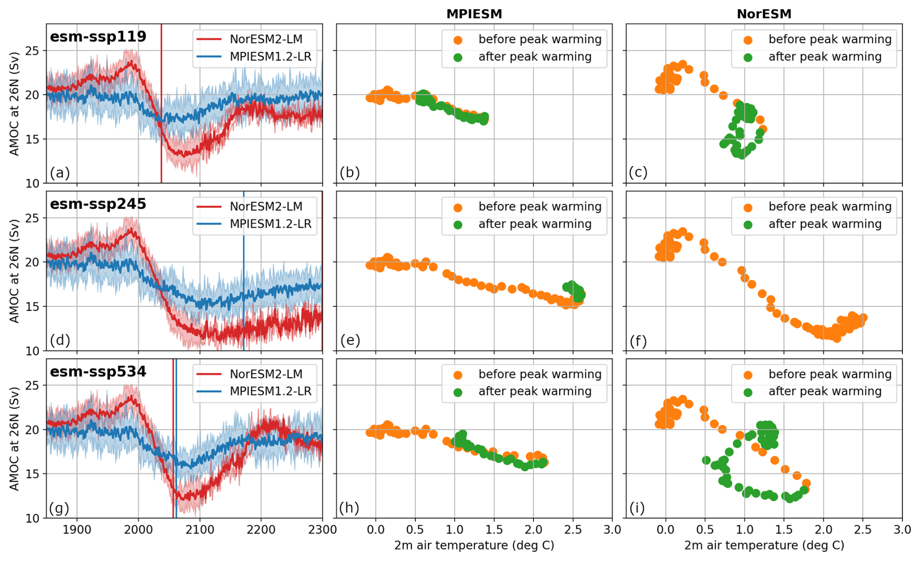
Figure 6 The evolution of the Atlantic Meridional Overturning Circulation (AMOC) index (a, d, g) over time and as a function of the global mean surface temperature (b, e, h: MPI-ESM1.2-LR; c, f, i: NorESM2-LM) in (a–c) esm-ssp119; (d–f) esm-ssp245; (g–i) esm-ssp534-over. In the left column, the years of peak warming are indicated for MPI-ESM1.2-LR and NorESM2-LM by a vertical line (in esm-ssp119 the two lines overlap and esm-ssp245 does not peak before 2300 in NorESM2-LM). In the temperature-AMOC plots, the color of the scatter points is changed after the year of the peak warming (green) compared to before (orange). The scatter plots use five-year averages for both variables.

NorESM2-LM shows a lag in its AMOC response rather than true irreversibility, but other components of the Earth system show true signs of irreversibility (Fig. 7) on the timescale of our experiments. Although global mean surface temperature (GSAT) stabilizes in the long run in esm-ssp534-over, the ocean continues to take up heat. A warmer ocean leads to the thermal expansion of seawater, contributing to sea-level rise (Wigley and Raper, 1987; Fig. 7a–c). A warmer ocean can also hold less dissolved oxygen (Oschlies et al., 2018; Fig. 7d–f) which can be detrimental to marine ecosystems.

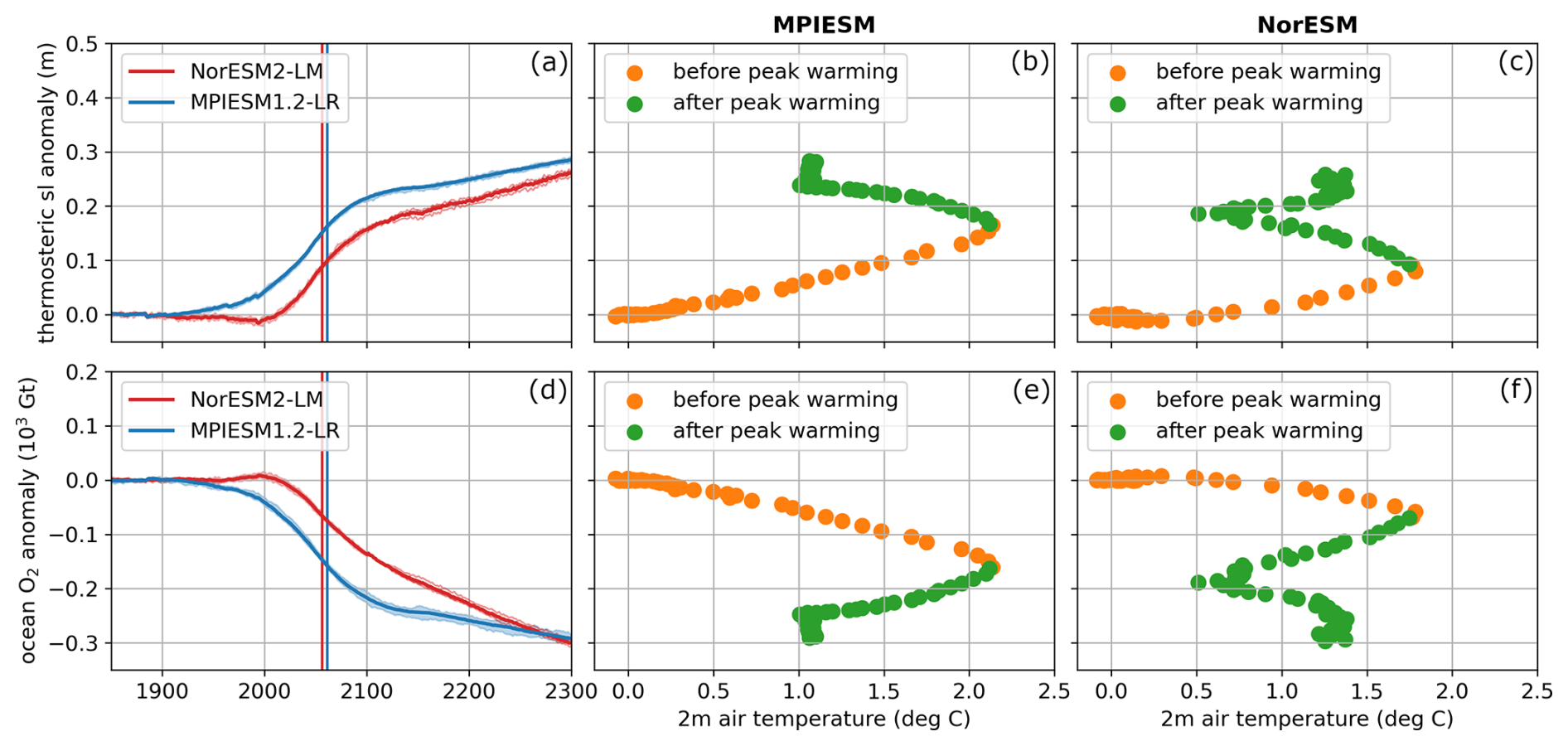
Figure 7 Irreversible global quantities of the Earth system in MPI-ESM1.2-LR and NorESM2-LM, inferred from the overshoot scenario esm-ssp534-over. (a–c) thermosteric sea-level rise; (d–f) Mass of oxygen in the ocean. In (a), (d), the vertical lines mark the year of peak warming and plots thermosteric sea-level rise and ocean oxygen mass as a function of time. The other columns plot these variables as a function of temperature in (b, e) MPI-ESM1.2-LR and (c, f) NorESM2-LM.

As for the AMOC response, interesting differences between the two ESMs can be observed for sea-level rise and de-oxygenation. After the historical period, sea-level increases monotonically and oxygen mass decreases monotonically in both models, regardless of whether global mean temperature smoothly peaks, declines and stabilizes (in MPI-ESM1.2-LR) or reaches a post-peak minimum before a second warming and stabilization (NorESM2-LM). Continued sea-level rise in overshoot scenarios has also been noted in previous studies with ESMs (Lacroix et al., 2024) and sea-level emulators (Nauels et al., 2025).

3.4 Regional signs of hysteresis and irreversibility

3.4.1 Temperature

We determine the regional climate characteristics at the same global warming level (GWL) in the esm-ssp534-over scenarios in both models.

Firstly, we observe that NorESM2-LM has four distinct phases in its global temperature evolution: a warming up until 2060, a cooling from 2060 to 2150, another warming from 2150 to 2200 and a stabilization from 2200 to 2300 (Fig. 3), qualitatively similar to the warming-cooling-warming cycles described in idealized NorESM2-LM overshoot simulations by Schwinger et al. (2022a). Taking the stabilization period as a 100-year mean GWL of 1.35 °C above pre-industrial (yellow shaded period in Fig. 8g), we apply this to the 31-year period around the crossing of this GWL in the warming (red shaded) and cooling (blue shaded) periods in Fig. 8g.

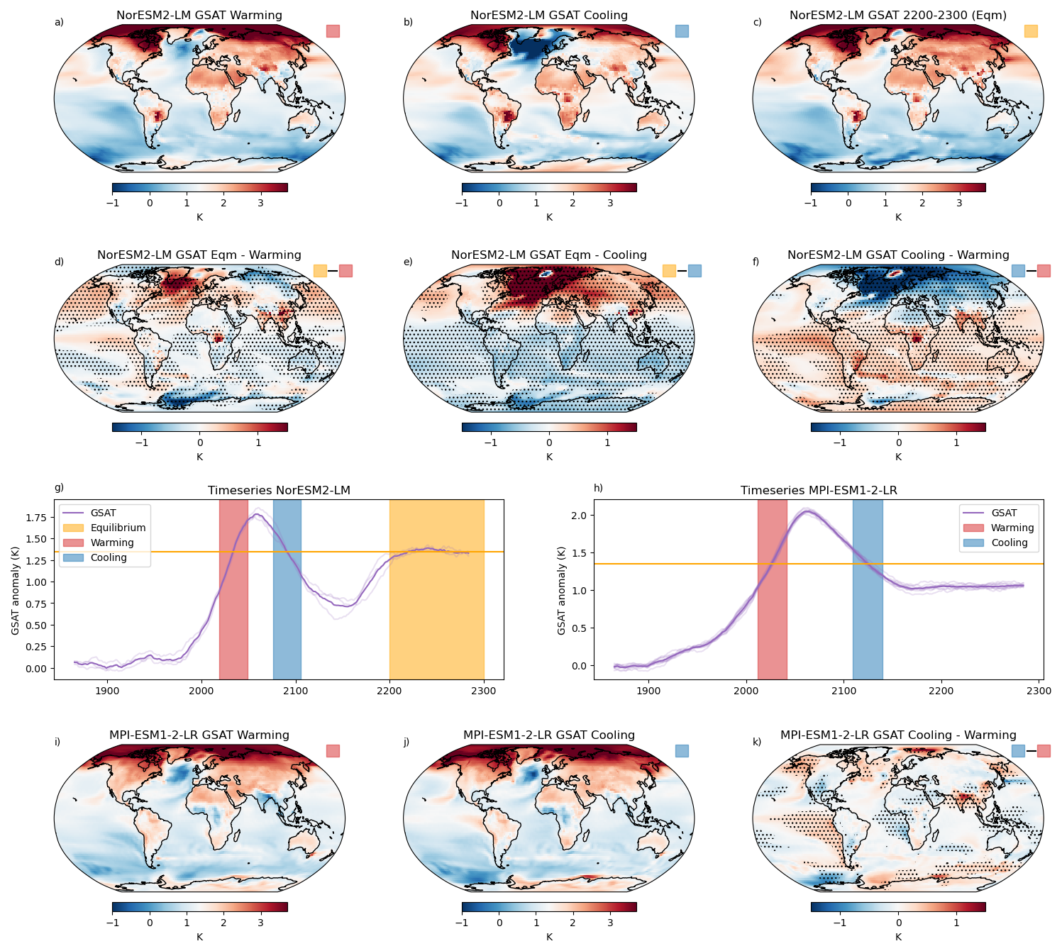
Figure 8 Global and regional near-surface air temperature projections in (a–g) NorESM2-LM and (h–k) MPI-ESM1.2-LR in the esm-ssp534-over scenario. (a–c) regional changes in NorESM2-LM for (a) warming; (b) cooling; (c) long-term stabilization around a 1.35 °C GWL. (d–f) Differences between (d) equilibrium and warming; (e) equilibrium and cooling; (f) cooling and warming in NorESM2-LM; (g, h) 31-year-smoothed timeseries of GSAT for (g) NorESM2-LM, showing times of warming (red), cooling (blue) and stabilization (yellow) at the 1.35 °C GWL and (h) MPI-ESM1.2-LR showing warming (red) and cooling (blue). (i–k) regional temperature at 1.35 °C GWL in MPI-ESM1.2-LR for (i) warming; (j) cooling, and (k) cooling minus warming. In (d–f) and (k), stippling shows areas where the differences are more than twice the standard deviation of the ensemble mean. In (g) and (h), red and blue shaded regions show the 31-year period around the ensemble mean 1.35 °C GWL, and individual ensemble members may use data from slightly earlier or later periods.

MPI-ESM1.2-LR shows three phases, where the first two are similar to NorESM2-LM and the third is a stabilization starting around 2150. We choose to compare the warming and cooling phases at the same 1.35 °C GWL used in NorESM2-LM, marked in red and blue respectively in Fig. 8h. Both Fig. 8g and h show a 31-year running mean of GSAT, centred on the year in the x axis.

The rest of Fig. 8 shows the regional patterns of warming at the 1.35 °C GWL. Figure 8a–c show the warming, cooling and stabilization periods in NorESM2-LM, and Fig. 8i and j in MPI-ESM1.2-LR. In these plots, red colours show regions warmer than the 1.35 °C GWL and blue marks regions cooler than 1.35 °C. In both models and all periods, the Arctic amplification and North Atlantic cold pool are distinct features, as is the contrast between land and ocean, where most land areas, particularly in the Northern Hemisphere, tend to be warmer than the global mean and ocean areas cooler than the global mean. Aside from the North Pacific and the Arctic, the ocean is also cooler than the global mean during the stabilization period. The strong cooling in the North Atlantic (where some regions are cooler than pre-industrial, despite the global mean warming being +1.35 °C) during the cooling phase of NorESM2-LM is consistent with the period of weakest AMOC (Fig. 6), showing the profound influence of the overturning circulation on transporting heat towards Western Europe.

Comparing differences between periods, we see that there is a more distinct asymmetry in regional temperatures between the cooling and warming phases in NorESM2-LM compared to MPI-ESM1.2-LR (Fig. 8f and k). NorESM2-LM loses heat from the Northern Hemisphere extratropics during the cooling phase, whereas the tropics and Southern Hemisphere are relatively warmer. In contrast, there are fewer regions of significant difference in MPI-ESM1.2-LR, suggesting that near-surface air temperature is more reversible in this model. While not directly comparable (analysing the stabilisation phase of an overshoot experiment relative to a zero-emissions commitment experiment), there is a diversity in hemispheric warming patterns post-net zero across the CMIP6 population (Cassidy et al., 2024; MacDougall et al., 2022) and therefore it is not surprising that the regional responses of the two models may differ.

The equilibrium period in NorESM2-LM is qualitatively different to both the warming and cooling periods. In equilibrium, the AMOC has recovered to a strength exceeding that of the warming phase, with enhanced oceanic heat transport resulting in a distinctly warmer Northern Hemisphere ocean (Fig. 8d). Other changes between equilibrium and warming are significant, but not as stark as the contrast between the equilibrium and cooling phases (Fig. 8e), where large hemispheric differences are apparent.

In contrast to NorESM2-LM, other CMIP6 models in the multi-model mean under ssp534-over have a warmer Southern Hemisphere and cooler Northern Hemisphere in equilibrium compared with the warming phase at approximately the same GWL (Roldán-Gómez et al., 2025a) as a consequence of a North-to-South transport of heat that commences at approximately the time of peak warming and persists into the 23rd century.

3.4.2 Precipitation

Figure 9 shows the global and regional patterns of precipitation for the warming and cooling phases at the 1.35 °C GWL.

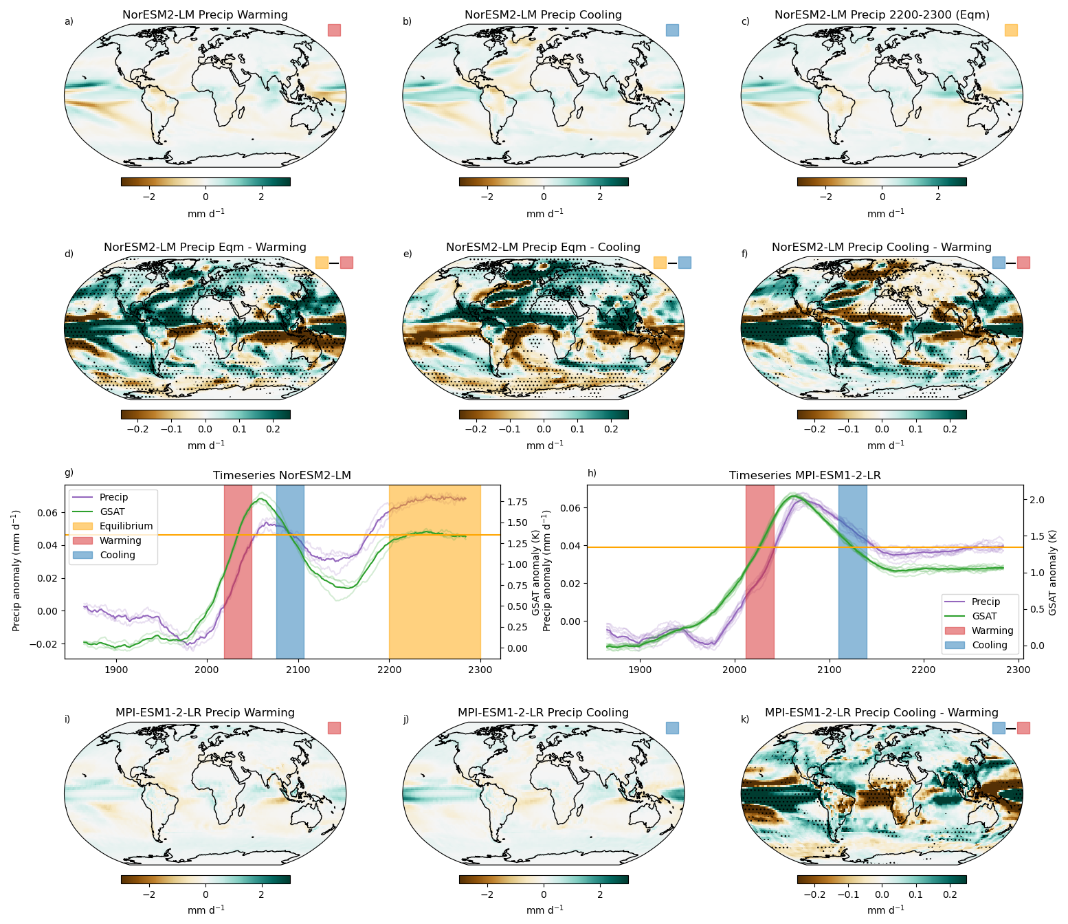
Figure 9 As Fig. 8, for precipitation. In (a)–(c) and (i), (j), anomalies are shown relative to pre-industrial. In (g) and (h), global means of both GSAT (green) and precipitation (purple) are shown.

In Fig. 9g and h, the global mean precipitation (purple curves) is shown superimposed on the GSAT anomaly (green curves). In both models, there is a lag in the response of global mean precipitation to global mean temperature, noting that precipitation response depends on the combination of climate forcers in addition to GSAT (Andrews et al., 2010). Both models project global mean precipitation in the cooling period to be higher than in the warming period, and in NorESM2-LM's case, the stabilization period is wetter still.

In both models during the warming phase, the inter-tropical convergence zone (ITCZ) shifts northward (Fig. 9a and i), which is consistent with the general hypothesis that the ITCZ moves towards the hemisphere with greater warming (refer to Fig. 8a and i), and other (concentration-driven) overshoot simulations from CMIP6 models Douglas et al. (2025); Kug et al. (2022). These differences persist in the cooling and stabilization phases (Fig. 9b, c, and j). Further analysing the differences in the phases, it can be noted that the ITCZ is northward shifted in the stabilization relative to warming, which also shows a generally wetter Northern Hemisphere (Fig. 9d). This is also true, though less clear, in the cooling minus warming differences in both models (Fig. 9f and k). Again, the equilibrium minus cooling phase in NorESM2-LM is interesting (Fig. 9e), with the ITCZ shifted southwards reflecting the relatively cooler Northern Hemisphere when comparing these two periods due to the weakened AMOC (Moreno-Chamarro et al., 2020). This results in a larger interhemispheric temperature gradient in the cooling phase in NorESM2-LM. This behaviour is consistent with the results of Steinert et al. (2025) for NorESM2-LM. Owing to the greater variability in precipitation, the regional changes are significant in a smaller proportion of the globe than for temperature.

Comparisons can again be drawn with other (concentration-driven) CMIP6 models for NorESM2-LM. In general, owing to the warmer Northern Hemisphere in the stabilization phase compared to warming phase, the ITCZ is more northerly located during the stabilization period (Fig. 9d), which is in contrast to the CMIP6 model mean (Roldán-Gómez et al., 2025a). However, NorESM2-LM shares the feature of increased precipitation in the eastern Pacific south of the equator with the CMIP6 model mean.

3.4.3 Net primary productivity

Finally, we demonstrate one aspect of the regional terrestrial carbon cycle response, the net primary productivity (NPP), which describes the amount of carbon taken up by photosynthesis minus the carbon loss through vegetation respiration.

In both models there is an overall net uptake in carbon in the land system relative to pre-industrial over all three future time periods (Fig. 10a–c and g–j), which is likely due to the CO₂ fertilisation effect. Nevertheless, some areas show a net carbon loss, including the region south-east of the Amazon (both models) and eastern North America (MPI-ESM1.2-LR).

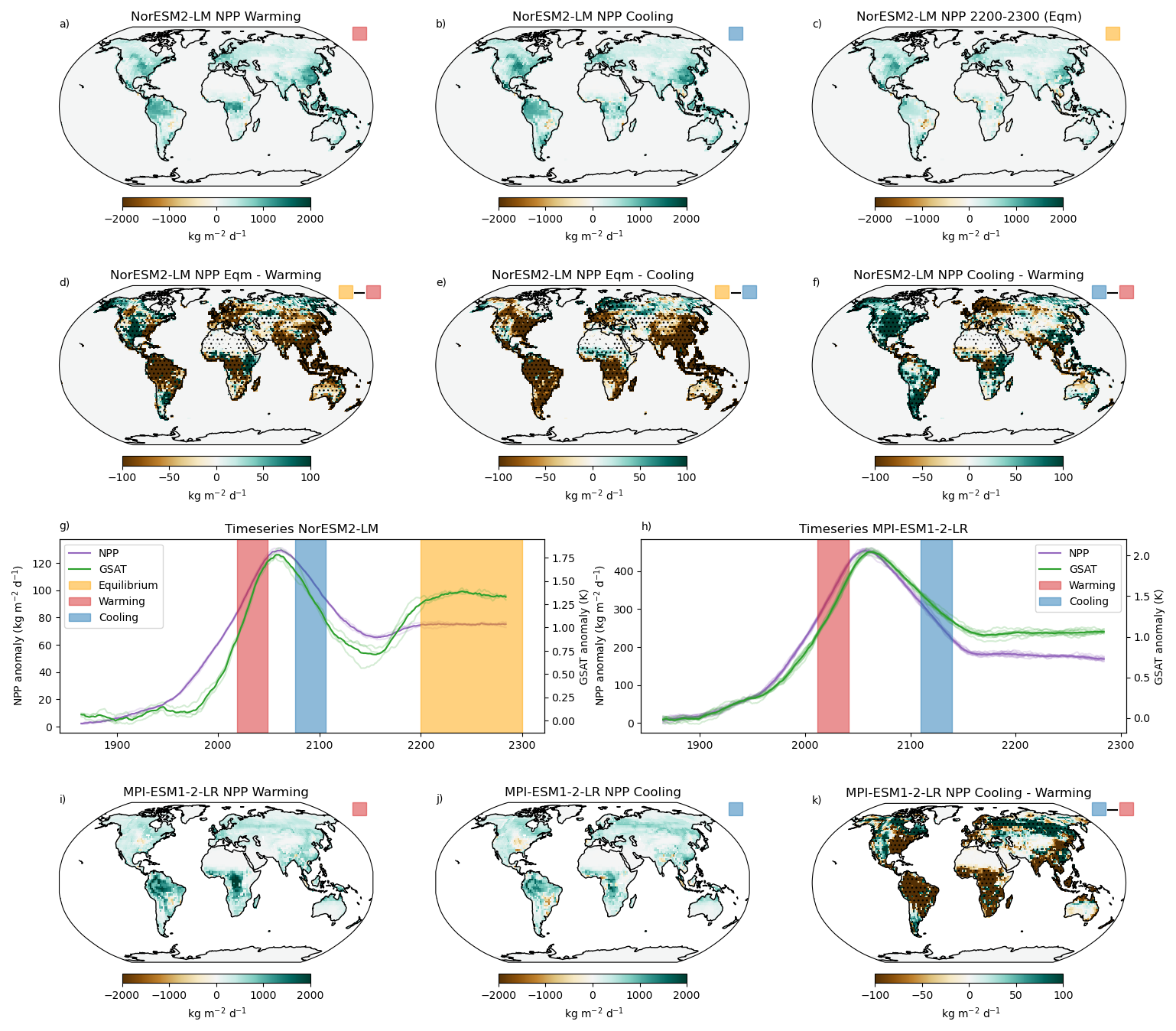
Figure 10 As Fig. 9, for net primary productivity. In (a)–(c) and (i), (j), anomalies are shown relative to pre-industrial. In (g) and (h), global mean GSAT anomaly (green) and total net primary productivity (purple) are shown.

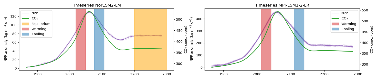
Furthermore, analysis of the global NPP shows that in the long term carbon sinks are not as productive at the same warming levels than they are in periods close to the start of the simulation (Fig. 10g and h). NPP more closely follows the evolution of atmospheric CO₂ than temperature (Fig. A1) which is related to the fertilisation effect, but this correspondence is not exact. There are also differences between the cooling and warming phases in both models. On the global scale, NorESM2-LM has higher NPP during the cooling phase than the warming phase, but MPI-ESM1.2-LR has lower NPP in the cooling phase relative to the warming phase. At the regional scale, NorESM2-LM (Fig. 10f) is taking up more carbon in North America but less in boreal Europe, whereas MPI-ESM1.2-LR is showing a reduced carbon uptake in the Amazon, eastern North America and sub-Saharan Africa, and an increase in Siberia (Fig. 10k).

4 Discussion and conclusions

We present two CO₂ emissions-driven ESMs run to 2300 under three different emissions scenarios: esm-ssp119 (a scenario designed to limit long-term warming to 1.5 °C with a small and temporary overshoot), esm-ssp245 (a roughly “current policies” scenario leading to around 2.5–3 °C warming in 2100) and esm-ssp534-over (a “high overshoot” scenario with very high greenhouse gas emissions in the short term and large amounts of carbon removal in the longer term). Each ESM has run multiple ensemble members for each scenario, which enables us to separate the forced signal from internal variability. The number of ensemble members required depends on the phenomenon being investigated: for global and regional mean state variables reported in this paper (temperature, precipitation, NPP, carbon fluxes and stocks, AMOC strength, thermosteric sea-level rise and ocean oxygen content) three members is likely sufficient to determine significant differences, though extremes (not evaluated in this paper) would benefit from a larger ensemble. We note several similarities and differences between the models. The two models have very different temperature responses, due to differences in the response of ocean circulation to climate forcing, especially for scenarios esm-ssp119 and esm-ssp534-over. Both NorESM2-LM and MPI-ESM1.2-LR peak in temperature in the 21st century, but while MPI-ESM1.2-LR declines and stabilizes thereafter, NorESM2-LM goes into a new warming phase that stabilizes in the 23rd century. Despite these differences, there are many responses that are similar in the two models. Considering esm-ssp534-over specifically we find that both models show:

1. a similar global distribution of anthropogenic carbon emissions among the atmosphere, ocean, and land. At the beginning of the simulations, most of the carbon remains in the atmosphere, but in the long term, the ocean becomes the dominant carbon reservoir;

2. a transition from carbon sink to carbon source: In both overshoot scenarios, both the land and ocean systems transition from being net carbon sinks to carbon sources around the year 2100. After 2150, the ocean resumes absorbing carbon, while the land continues to release carbon to the atmosphere;

3. a similar global response of precipitation to temperature changes, where global precipitation is higher during the cooling phase than during the warming phase;

4. a northward shift of the ITCZ during the warming phase, with similar patterns being observed during the cooling and stabilization phases;

5. long-term irreversibility in sea level and ocean deoxygenation, which are largely irreversible even after temperatures decline on the timescales of these simulations.

In contrast, there are differences in the global and regional responses to CO₂ emissions between the models resulting from varying sink strengths in the global carbon cycle and patterns of ocean warming. NorESM2-LM shows substantial hysteresis in its AMOC strength and regional patterns of warming when comparing periods before and after peak warming. MPI-ESM1.2-LR is more reversible in its AMOC and regional pattern of warming. While the main focus of our analysis of irreversibility was the esm-ssp534-over simulations, we note qualitatively similar behaviour for the smaller overshoot esm-ssp119 scenario for global temperature as a function of emissions. We find a similar pattern of regional temperature and precipitation response to periods before and after peak warming in the MPI-ESM1.2-LR model to concentration-driven scenarios in Pfleiderer et al. (2024), indicating that physical climate responses are likely not sensitive to whether scenarios are run with prescribed emissions or concentrations.

While esm-ssp534-over was designed as a relatively extreme narrative to test the responses of ESMs to negative emissions, a large class of emissions scenarios that peak warming in the 1.5–2.0 °C range before declining towards the end of the 21st century were submitted by IAM teams to the IPCC Sixth Assessment Report (Riahi et al., 2022). It is very likely that overshoot is required to limit global mean warming to 1.5 °C in the long term due to a lack of action on greenhouse gas emissions reductions in the last decade (Schleussner et al., 2024). Therefore, given the diversity of the responses of these two models to these scenarios, further investigation should target a larger set of models and additional overshoot pathways.

From a peak global mean temperature perspective, the results presented in this paper probably represent a “best case” scenario. Both models have a (150-year Gregory regression-derived) climate sensitivity on the low side of the CMIP6 range, and have a strongly negative ZEC meaning that temperatures are expected to cool after net zero CO₂ is reached (MacDougall et al., 2020), notwithstanding the influence of non-CO₂ forcers. The esm-ssp119 simulations peak below 1.5 °C in both models and are likely biased cool relative to historical GSAT change. The combination of low (Gregory) climate sensitivity, strong negative ZEC, and potential low-biased ensemble mean warming levels mean that the outcomes presented in the paper may underestimate the risks and challenges associated with overshoot scenarios. In addition, while on the cool side in terms of GSAT, the projections from NorESM2-LM suggest that large abrupt changes in AMOC, rapid phase of warming during the late 22nd century, and substantial regional changes such as cooling in Europe during the slowdown phase may pose more severe adaptation challenges than a model with higher peak warming but a more reversible regional climate profile. In reality, the Earth system's response could be more severe, with greater irreversibility and fewer opportunities for recovery. In order to sample the full range of plausible futures in response to CO₂ emissions, more participating models running several different CO₂ emissions-driven scenarios, with and without overshoot, are required (Sanderson et al., 2024). Even within our two-model ensemble we see very different long-term behaviours, and NorESM2-LM suggests that the risks of AMOC slowdown and regional cooling over Europe, as well as an unexpected warming rebound once negative emissions cease, cannot be ruled out.

Appendix A

Figure A1 As Fig. 10g and h, showing the global total net primary productivity (purple) compared to the global mean CO₂ concentration (green) in NorESM2-LM (left) and MPI-ESM1.2-LR (right).