Climate models with moderate climate sensitivity best simulate the magnitude of Earth's energy imbalance

Recent studies have highlighted that state-of-the-art climate models are not able to simulate the large observed trend in Earth's energy imbalance. Here we evaluate climate models' ability to represent both the trend and the magnitude of the imbalance, while accounting for model energy leakage and remnant drift. As reference we use satellite observations and we find that every observed annual mean energy imbalance is within the range simulated by models, including the record year 2023, and when averaged over the 2001–2025 period, 13 out of 30 models simulate magnitudes of the imbalance that are statistically consistent with the observations. Models, however, generally underestimate the positive trend in the energy imbalance, albeit barely within the range of uncertainty. We suspected that a discontinuity in volcanic forcing between the historical and future scenario in 2014–2015 could have caused the underestimated trend, but only found evidence of such artifacts for a few models. Finally, we find a weak correlation between short-term decadal warming and energy imbalance, but a surprisingly close relationship between energy imbalance and equilibrium climate sensitivity. Based on observational constraints, the relationship suggests that models with climate sensitivities of 3 to 5 K best simulate the observed energy imbalance.

1 Introduction

Earth's energy imbalance, expressed as the difference between incoming solar and outgoing radiation at the top-of-atmosphere, is one of the most fundamental metrics of the climate system (Fourier, 1822; Arrhenius, 1896; Manabe and Strickler, 1964; Hansen et al., 2011; von Schuckmann et al., 2023). Today, the climate system is out of balance, mainly due to anthropogenic greenhouse gas emissions (Houghton et al., 2001), and a positive trend in the Earth's energy imbalance has been evident in satellite observations in recent decades (Loeb et al., 2024). The climate science community has indicated that the imbalance is rising faster than expected, and climate models underestimate the observed trend (Raghuraman et al., 2021; Hodnebrog et al., 2024; Olonscheck and Rugenstein, 2024; Mauritsen et al., 2025; Myhre et al., 2025). In this study we evaluate the performance of global climate models in simulating both the trend and the magnitude of the Earth's energy imbalance.

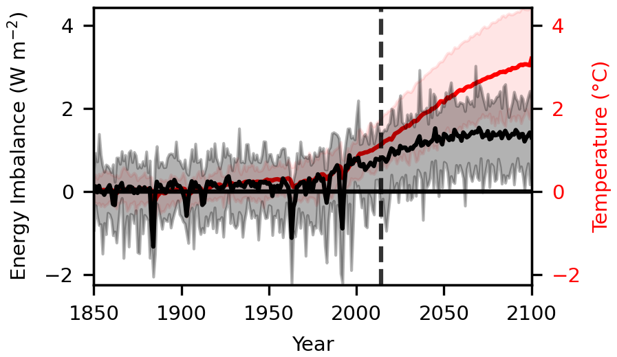
Figure 1 Energy imbalance (black line) and range of minimum and maximum imbalance in CMIP6 ensemble members (grey shaded). Near-surface air temperature (red line) and ensemble range (red shaded area). The vertical dashed line corresponds to the transition year (2014) between the historical experiment and the SSP2-4.5 scenario.

The value of observing the imbalance trend is indispensable for both science and climate policy. By definition the imbalance trend is the rate of change of accumulated energy in the climate system, so in a broad sense this trend determines the pace of global warming, with 89 % of the excess heat stored in the ocean, 6 % on land, 4 % in the cryosphere while 1 % ends up within the atmosphere (von Schuckmann et al., 2023). Specifically, the imbalance leads to rising temperatures, rising sea level, and more extreme weather (von Schuckmann et al., 2016). Climate models that run the Shared Socioeconomic Pathway (SSP) 2-4.5 scenario reveal an increase in the imbalance, reaching a nearly constant level in the second half of the 21st century, while the temperature continues to rise through 2100 surpassing 3 °C (Fig. 1). Under more stringent mitigation scenarios that limit global warming to less than 2 °C, the energy imbalance is expected to peak already in the 2030s, several decades before the surface temperature stabilises (Mauritsen et al., 2025). Thus, Earth's energy imbalance can act as an indicator of future temperature change as a result of anthropogenic activity.

The Earth's energy imbalance (N) is influenced by a number of factors, including radiative forcing, feedbacks and internal variability. In a linearised framework the change in imbalance N can be expressed as:

$$\begin{array}{}\text{(1)}& N=F+\mathit{\lambda }\mathrm{\Delta }{T}_{\mathrm{s}}+\mathit{ϵ}\end{array}$$

in relation to the radiative forcing F, the feedback λ in response to global mean surface temperature change ΔT_s and the internal variability of the system ϵ, such as random weather events and unforced temperature pattern effects. The three terms result from distinct processes:

• The dominant forcing originates from increased concentrations of greenhouse gases, primarily CO₂. Furthermore, anthropogenic aerosol emissions result in a negative forcing that translates to a cooling effect, due to an increase in the reflected shortwave radiation to space. There is considerable uncertainty in the strength and evolution of the aerosol cooling (Bellouin et al., 2020; Forster et al., 2021). However, there is evidence for a weakly decreasing aerosol cooling effect during approximately the past 20 years (Quaas et al., 2022; Forster et al., 2025), and this has contributed to the upward trend in simulated energy imbalance (Hodnebrog et al., 2024), while using reanalysis and observations Park and Soden (2025) show that aerosol-radiation and aerosol-cloud interactions have minimal impact on the energy imbalance trend.

• The equilibrium climate sensitivity (ECS) of the system, which is the long-term temperature increase in response to a doubling of the atmospheric CO₂ concentration relative to pre-industrial values, can be defined in relation to the total feedback parameter λ and the equivalent forcing $F_{\mathrm{2}\times {\text{CO}}_{\mathrm{2}}}$:

  $$\begin{array}{}\text{(2)}& \text{ECS}=-{\displaystyle \frac{F_{\mathrm{2}\times {\text{CO}}_{\mathrm{2}}}}{\mathit{\lambda }}}\end{array}$$

  A large negative λ is associated with a low climate sensitivity. As can be seen from Eq. (1), a large negative λ results in a strong dampening of the energy imbalance when temperatures rise, and Myhre et al. (2025) argue that low climate sensitivity models are not able to reproduce the trend in the shortwave component of the energy imbalance. Therefore, a high climate sensitivity is another candidate explanation for the rise in the energy imbalance.

• Finally, internal variability may be involved in causing the large trend in the Earth's energy imbalance, although it should be pointed out that internal variability alone cannot fully explain the observed trend without changes in external forcing (Raghuraman et al., 2021). Internal variability at the global scale can be caused both by atmospheric processes that lead to variations in the energy imbalance and by exchange of energy with the deep ocean, by as much as ±0.2 Wm⁻² on average over 15-year periods (Hedemann et al., 2017). Thus, internal variability can be an important factor when assessing the model-simulated magnitude and trend of the energy imbalance.

The central focus of this study is to evaluate models from the Coupled Model Intercomparison Project Phase 6 (CMIP6) regarding the simulation of both the magnitude and the trend of the energy imbalance (Sect. 3). For this purpose, we subtract the pre-industrial control experiment imbalance to account for energy leakage and remnant model drifts (Sect. 2). We explore whether the implementation of volcanic aerosols in the future scenario could have played a role in the underestimated trend (Sect. 4). Finally, we investigate the relationship between the present-day imbalance and short-term to long-term global warming (Sect. 5).

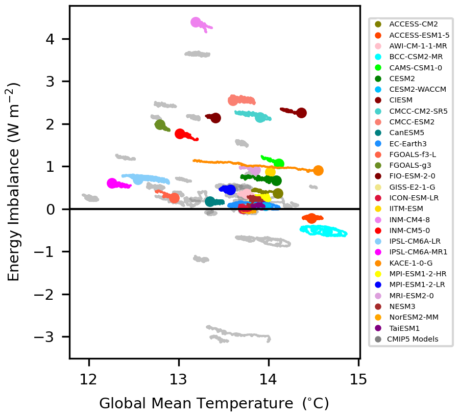
Figure 2 Energy imbalance versus near-surface air temperature for the piControl experiment. Lines correspond to the 50-year running mean of the full piControl simulation for CMIP6 models (colours) and CMIP5 models (grey). Circles correspond to the mean of the last 50 years.

2 Data and Methods

2.1 Observations

We use data from the Clouds and Earth's Radiant Energy System (CERES) mission as our observational reference, with complementary reconstructed data to extend our analysis period further back in the past. For the period 2001–2025, we use the CERES energy-balanced and filled (EBAF) product, version 4.2.1 (NASA/LARC/SD/ASDC, 2023; NASA, Langley Research Center, 2025). This data product combines radiation budget data from multiple satellites, which are known to have a bias of several Wm⁻² in the global annual mean before adjustments (Fig. A1). These data are adjusted within their uncertainties to match the global annual mean imbalance for 2005-2015 as determined from measurements of ocean heat content, so that the final EBAF data do not exhibit this bias (Loeb et al., 2018).

For the period 1985–2000, we use data from the Diagnosing Earth's Energy Pathways in the Climate system (DEEP-C) project version 5.0, which is based on satellite observations from the Earth Radiation Budget Satellite (ERBS), CERES, atmospheric reanalysis from the European Centre for Medium-Range Weather Forecasts (ERA5) and model simulations from the Atmospheric Model Intercomparison Project in CMIP6 (Liu and Allan, 2022). The use of reanalysis along with the merging process results in considerable uncertainty of the data (Liu et al., 2020). We refer to the combined 1985-2025 dataset as CERES EBAF extended.

As for temperature observations, the HadCRUT5 Analysis version 5.1.0.0 dataset from the Met Office Hadley Centre Climatic Research Unit, University of East Anglia is used (Morice et al., 2021).

2.2 Model experiments

We use output data from 239 ensemble members of 30 climate models participating in CMIP6 (Eyring et al., 2016). The models are listed in Table A1. In our analysis we combine the historical experiment from 1850 to 2014 with the SSP2-4.5 scenario from 2015 to 2100 to produce time series of the annual global mean imbalance and near-surface air temperature from 1850 to 2100.

The top-of-atmosphere energy imbalance of a model that perfectly conserves energy is expected to be close to zero after the model has been run for thousands of years. However, most models do not perfectly conserve energy and some models are also drifting in their piControl experiments (Mauritsen et al., 2012). Figure 2 shows the individual model energy imbalance values of the piControl experiment ranging from about −3 Wm⁻² to more than 4 Wm⁻². In this experiment, where the model is expected to be in a steady state, a positive energy imbalance corresponds to energy leakage, and a negative energy imbalance is associated with an artificial input or source of energy. To account for this, we adjusted the imbalance time series to compensate for both artificial energy leakage and remnant drift by subtracting the global time-mean imbalance found in the piControl experiment for each model. It is noted that the drift in energy imbalance in these 500 years or longer piControl experiments is relatively small, on the order of 0.1 Wm⁻² in most models, such that the error caused by assuming a constant leakage is negligible.

2.3 The two-layer model

As outlined in the introduction, we expect a relationship between the simulated energy imbalance and climate sensitivity. To explore this relationship we will apply the widely used two-layer model with a pattern effect (Winton et al., 2010; Armour et al., 2013; Geoffroy et al., 2013; Rohrschneider et al., 2019):

$$\begin{array}{c}{\displaystyle }C{\displaystyle \frac{\mathrm{d}T}{\mathrm{d}t}}=F+\mathit{\lambda }T-\mathit{\epsilon }\mathit{\kappa }(T-T_{\mathrm{d}})\\ {\displaystyle }{C}_{\mathrm{d}}{\displaystyle \frac{\mathrm{d}{T}_{\mathrm{d}}}{\mathrm{d}t}}=\mathit{\kappa }(T-T_{\mathrm{d}})\\ {\displaystyle }N=C{\displaystyle \frac{\mathrm{d}T}{\mathrm{d}t}}+C_{\mathrm{d}}{\displaystyle \frac{\mathrm{d}{T}_{\mathrm{d}}}{\mathrm{d}t}}\end{array}$$

where N is the energy imbalance, F the effective radiative forcing, λ the feedback parameter, C and C_d are the heat capacities of the upper and deep layers, T and T_d the respective temperatures, ε the ocean heat uptake efficacy used to represent the forced pattern effect, and κ is the deep ocean heat uptake coefficient. The parameters ε=1.3 and κ=0.7 Wm⁻² K⁻¹ are chosen such that when ECS is set to 3.0 K the transient climate response (TCR) is approximately 1.8 K, which are the combined assessed best estimates of Forster et al. (2021). The model is driven by the historical and SSP2-4.5 best-estimate effective radiative forcing time series (Smith et al., 2021).

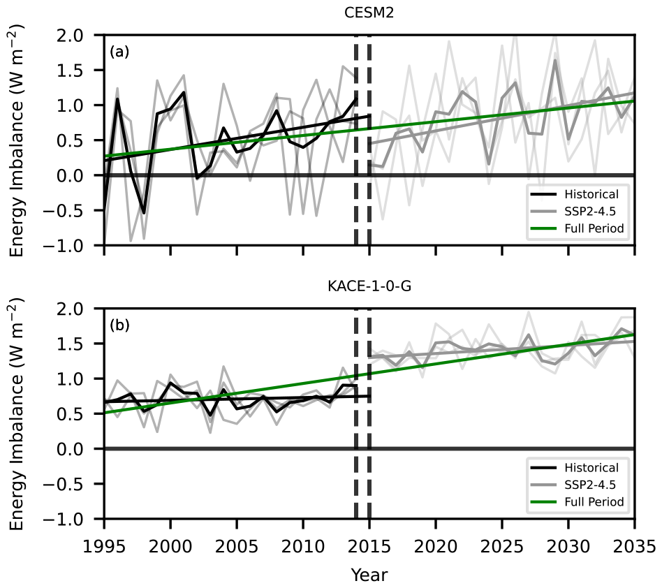
Figure 3 Energy imbalance in CMIP6 models CESM2 (a) and KACE-1-0-G (b) for 1995–2035. Time series of the historical experiment for 1995–2014 (black) and SSP2-4.5 future scenario for 2015–2035 (grey) along with a linear regression for each time period and the full time period (green). Year of transition between the two experiments in 2014–2015 (black dashed vertical lines).

2.4 Magnitude, trend and confidence intervals

We compute the imbalance magnitude and trend along with 5 %–95 % confidence intervals for both quantities, for observations and models. The magnitude of the imbalance is calculated as the time mean over the selected time period, while the trend in the imbalance is quantified as the slope of a linear regression of the annual global mean values. In the case of models with only one realisation, as well as for the single time series of observational reference data, these two quantities are straightforward to compute. In the case of models with multiple ensemble members, the magnitude and trend are first calculated separately for each member, and the mean of those values are used to represent the model. Uncertainties are presented as 5 %–95 % confidence intervals (CI), which are computed using a standard error σ:

$$\begin{array}{}\text{(3)}& \mathrm{CI}=\pm \mathrm{1.64}\times \mathit{\sigma }\end{array}$$

The standard error is computed slightly differently for different models and for observations. For models with only a single realisation, the standard error in the imbalance magnitude is computed directly from the annual time series, after first removing the linear trend over the period. The standard error in the imbalance trend is given by the corresponding linear regression. For models with multiple realisations, we use the mean of the standard errors calculated for the individual realisations. It is worth clarifying that the focus of our analysis is on the range of values that each model can simulate, rather than on the expected forced response of each model. Therefore we do not compute the standard error for a given model by dividing the quantity by the square root of the number of realisations, but instead use the mean of the standard errors for each realisation. The standard error in the observation-based imbalance magnitude is computed in the same way as for the single-realisation models, and furthermore the standard error in the observed trend additionally includes the effect of an explicit observational uncertainty σ_obs. Specifically, we use σ_obs=0.1 Wm⁻² decade⁻¹ and combine this with the standard error from a linear regression σ_reg as in Raghuraman et al. (2021) for the CERES EBAF product, but here we also include the same observational error for the CERES EBAF extended dataset for simplicity:

$$\begin{array}{}\text{(4)}& \mathit{\sigma }=\sqrt{{\mathit{\sigma }}_{\text{reg}}^{\mathrm{2}}+{\mathit{\sigma }}_{\text{obs}}^{\mathrm{2}}}\end{array}$$

2.5 Difference in imbalance in the transition between experiments

To investigate how the overall calculation of the trend might be affected by the transition from the historical experiment to the SSP2-4.5 future scenario (Sect. 4), we quantify the difference in imbalance and clear-sky components of the net shortwave and longwave radiation at the transition year 2015. We perform linear regressions for the periods immediately before (1995–2014) and after (2015–2035) the transition. Data from the historical experiment are used from 1995 to 2014, with an extrapolation for 2014–2015, while data from the SSP2-4.5 scenario are used from 2015 to 2035. To illustrate the method we show two examples in Fig. 3. For CESM2 there is a strong upward trend before and after the transition, but the negative shift leads to a weaker overall trend. For KACE-1-0-G there is a near-zero trend before and after the transition, but the upward shift, as we shall see, leads to this model exhibiting the largest trend in the simulated energy imbalance.

2.6 Climate sensitivity

Climate sensitivity values are retrieved from Myhre et al. (2025), derived from abrupt 4xCO₂ simulations over 150 years. Following Gregory et al. (2004), they calculate the effective climate sensitivity through regression of the energy imbalance and surface temperature in CMIP6 models. Because Myhre et al. (2025) do not include the CMCC-CM2-SR5 and CMCC-ESM2 models, we also exclude these models in Sect. 5.

3 Evaluation of CMIP6 modelled energy imbalance magnitude and trend

The evolution of the energy imbalance simulated by CMIP6 models was introduced earlier for the complete time series (Fig. 1), and in the following paragraphs we focus on the time period in which satellite observations are available.

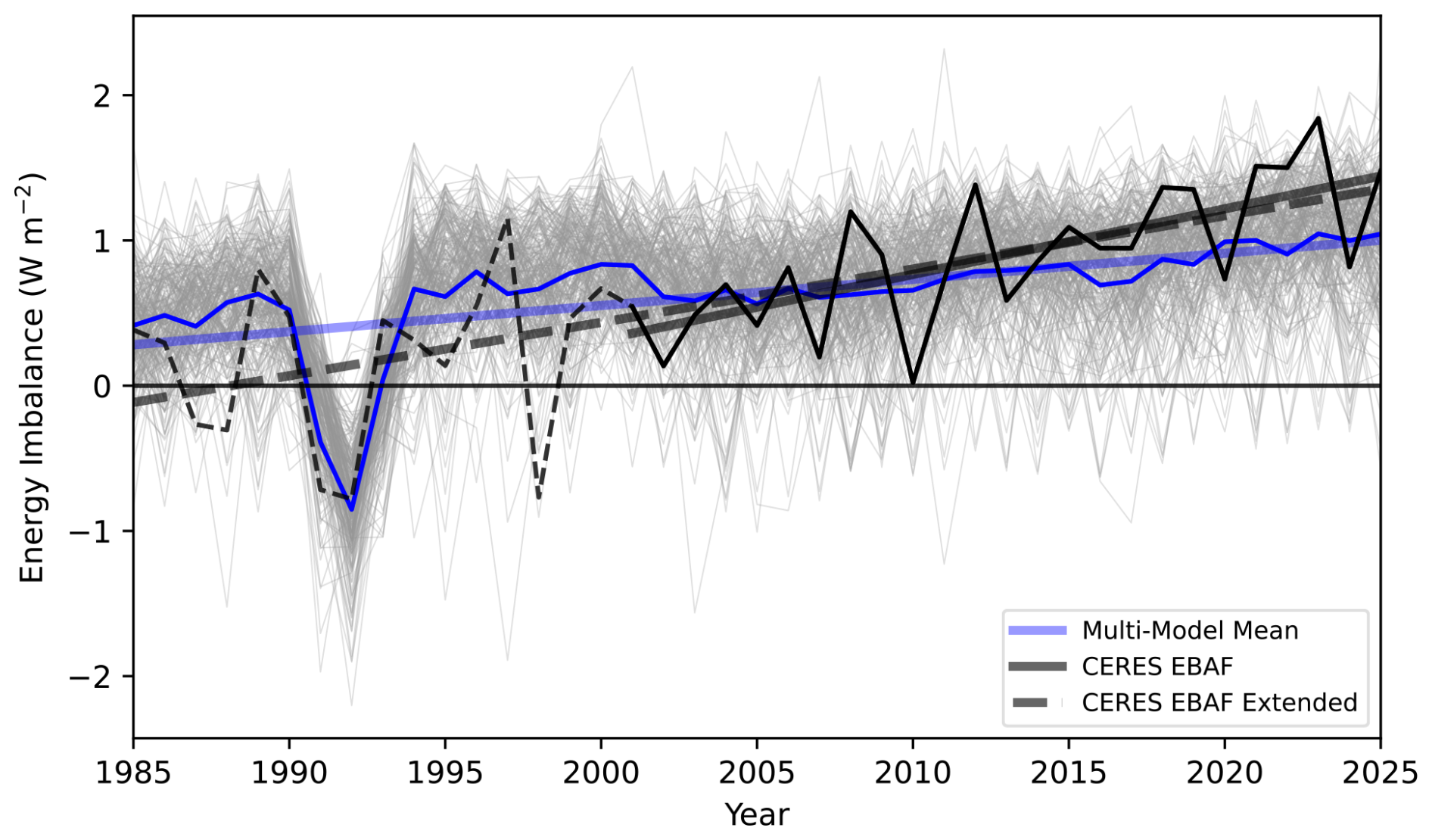
Figure 4 Energy imbalance simulated by CMIP6 models (grey lines) along with the multi-model mean imbalance and regression line (blue). The CERES EBAF values for the energy imbalance (black line) are also shown, in addition to the CERES EBAF Extended with DEEP-C data (dashed black line).

First, when inspecting the full time series we find that model-simulated values of the energy imbalance in the beginning of the observational time period are higher than those observed, whereas the opposite is the case in the end of this period (Fig. 4). As a result the trend in the observed imbalance is steeper than in the multi-model mean. Variability of the annual mean imbalance is evident within the different ensemble members, with some of the members simulating values ranging from about −2.0 Wm⁻², mainly during and right after the 1991 Pinatubo eruption, up to more than +2.0 Wm⁻² in some other years. All the observed annual means, including the record peak value of 1.8 Wm⁻² in 2023, are within the range simulated by the CMIP6 ensemble members. The fact that the model range captures the peak observations is related to internal variability. For comparison Myhre et al. (2025) found that the 2023 CERES EBAF value is higher than that of any of the CMIP6 models, but their study uses a single realisation for each model.

Second, we evaluate the temporal mean magnitude by comparing CMIP6 simulated values with the CERES EBAF data (Fig. 5). Our results indicate a good agreement between models and observations, and specifically 13 out of the 30 models are in agreement with the observational data within the 5 %–95 % confidence interval. Two models simulate values above, while 15 models are below the observational confidence interval. An alternative is to use the model estimated confidence intervals, which vary substantially between models due to different levels of internal variability. Nevertheless, in this case a slightly different subset of 13 models have confidence intervals that overlap with the CERES EBAF mean. It is worth noting that even though many models are consistent with the observed magnitude of the energy imbalance, Fig. 4 shows that this is partly the result of larger simulated values at the beginning of the period, combined with smaller than observed model simulated values towards the end of the time period.

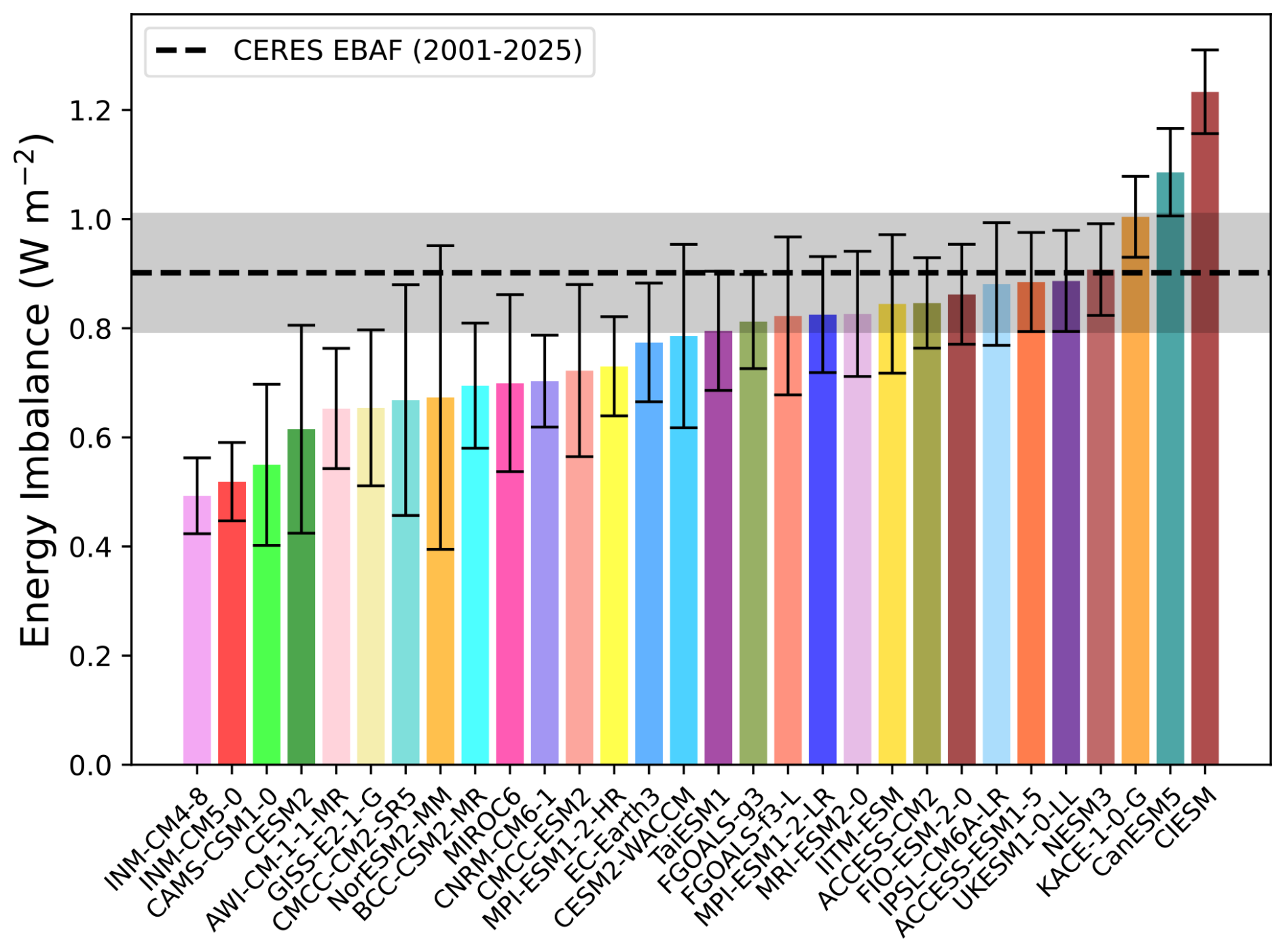
Figure 5 Energy imbalance magnitude of CMIP6 models (coloured bars) and observations (dashed black line) for the 2001–2025 CERES EBAF time period. The error bars for the models and the grey shaded area for the observational data correspond to the 5 %–95 % confidence interval.

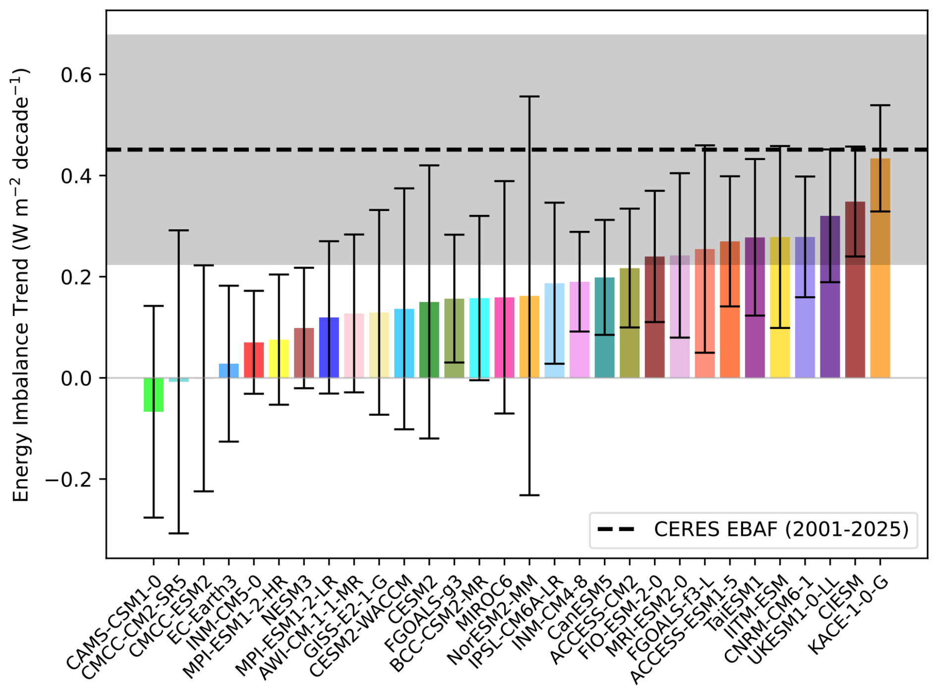
Figure 6 Energy imbalance trend of CMIP6 models (coloured bars) and observations (dashed black line) for the 2001–2025 CERES EBAF time period. The error bars for the models and the grey shaded area for the observational data correspond to the 5 %–95 % confidence interval.

Third, we turn to the CMIP6 simulated trend of the energy imbalance. In line with earlier studies (Raghuraman et al., 2021; Hodnebrog et al., 2024; Myhre et al., 2025), we find that the majority of the models fail to reproduce the large observed trend in the energy imbalance (Fig. 6). The individual models exhibit a wide range in their calculations of the trend: Of the 30 CMIP6 models considered in this study, 10 are consistent with the observational confidence interval, while 1 model has zero trend and 2 models even simulate negative trends in their energy imbalance. If we instead use the individual model confidence intervals only 6 of them show an overlap with the CERES EBAF mean trend. This difference in the number of models that are consistent is partly due to varying internal variability in the models and the inclusion of measurement uncertainty in the observational confidence interval (Eq. 4). Regardless of how it is viewed, however, it seems clear that the majority of models are not simulating trends that are consistent with the CERES EBAF observations.

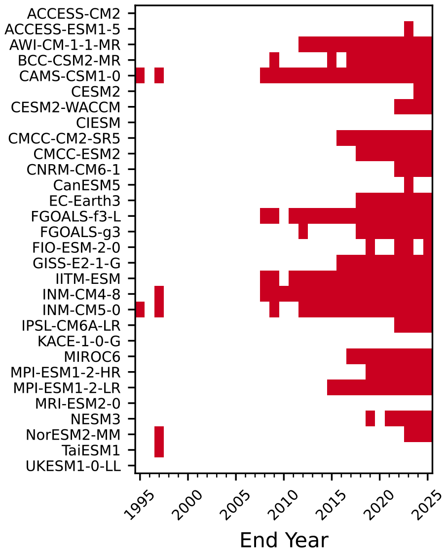
Figure 7 Agreement between CMIP6 models and CERES EBAF Extended observational data. Agreement (white shaded area), when the ensemble mean value of the energy imbalance trend lies within the 5 %–95 % confidence interval of the observations. By contrast, disagreement (red shaded), when the model ensemble mean of the energy imbalance trend falls outside the 5 %–95 % confidence interval.

To investigate these trend results further, we evaluate CMIP6 model performance regarding the trend of the energy imbalance compared with all available observational data using two separate approaches. For both methods, 1985 is chosen as the baseline year, and the trend of the energy imbalance is computed over increasingly longer intervals, for consecutive end years of the time series from 1995 to 2025. Thus, the shortest trend is calculated over 11 years and the longest over 41 years.

In the first approach, we evaluate model performance in a binary way of categorization, using an agreement/disagreement method in which each individual model is considered consistent with observations when the model ensemble mean calculated trend (Sect. 2.4) falls within the 5 %–95 % confidence interval of the observations. Initially, as illustrated in Fig. 7, agreement is found for most of the CMIP6 models, with a few exceptions in the beginning of the time period. This is only natural as 10 % of the models should be outside the 5–95 percentiles of the observations. However, a nearly continuous disagreement is apparent in several models starting in 2008, and for trends calculated over the entire 1985–2025 period, 22 of the 30 models are inconsistent with the observations.

In the second approach, we use the entire set of individual model ensemble members and evaluate the observational data relative to the full spread of the models (Fig. 8). We find that the energy imbalance trend derived from the observational data lies mostly within the range of the CMIP6 ensemble members. However, from 2014 onwards the observed calculated trend is found to be at the upper bound of the model ensemble range, on the verge of exceeding the maximum values of the CMIP6 ensembles. Consequently, both of these methods indicate that many models fail to reproduce the observed trend after about 2010–2015.

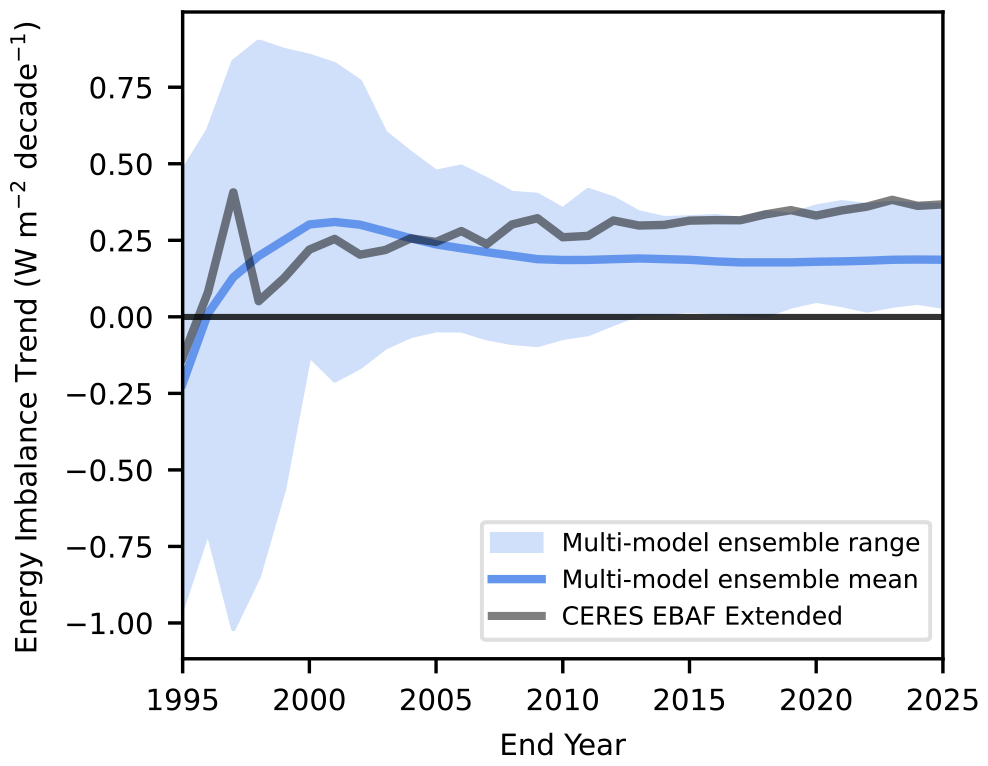
Figure 8 Energy imbalance trend per decade for starting year in 1985 and for consecutive end years from 1995 to 2025. The blue shaded area corresponds to the minimum and maximum of the ensemble members of CMIP6, the blue line is the ensemble mean, and the grey line refers to the CERES EBAF extended observational dataset.

All in all, we can say that (1) on an individual annual mean basis, none of the observations are outside the range simulated by CMIP6 models, (2) the magnitude of the observed imbalance is also in line with CMIP6 models, but (3) most models systematically underestimate the observed trend. In the next section we will investigate whether the underestimated trend in recent years can be caused by implementation issues when going from the historical to future scenario experiments.

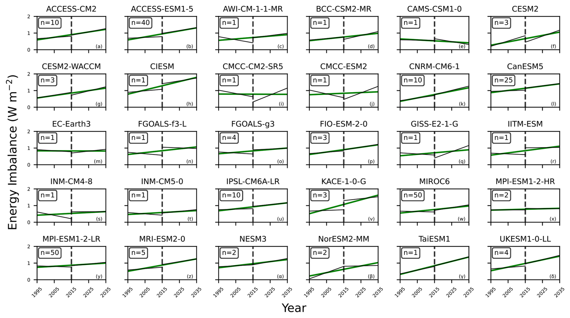
Figure 9 Linear fits (black) to the energy imbalance on 20-year time intervals before and after the year of transition (2015) from the historical experiment to the SSP2-4.5 scenario for the CMIP6 models. Green lines show linear fits on the combined 1995–2035 period.

4 A potential source of the CMIP6 underestimated trend

Here, we investigate one possible cause, related to volcanic aerosol forcing in the future scenario, that could be responsible for the underestimation of the CMIP6 simulated energy imbalance trend in recent decades. Our idea is that the introduction of a constant background volcanic aerosol in future scenarios from 2015 onward, following the CMIP6 experimental protocol as described by O'Neill et al. (2016), would manifest as a negative shift or discontinuity in the imbalance between 2014 and 2015. Because the average historical volcanic aerosol loading is larger than the actual loading during 2015–2025, implementing this would have a negative impact on the model-simulated energy imbalance trend, and to a lesser extent also result in a lower magnitude of the energy imbalance. A discrepancy attributable to the volcanic aerosol forcing in the future scenarios should be most evident in the clear-sky component of the shortwave radiation.

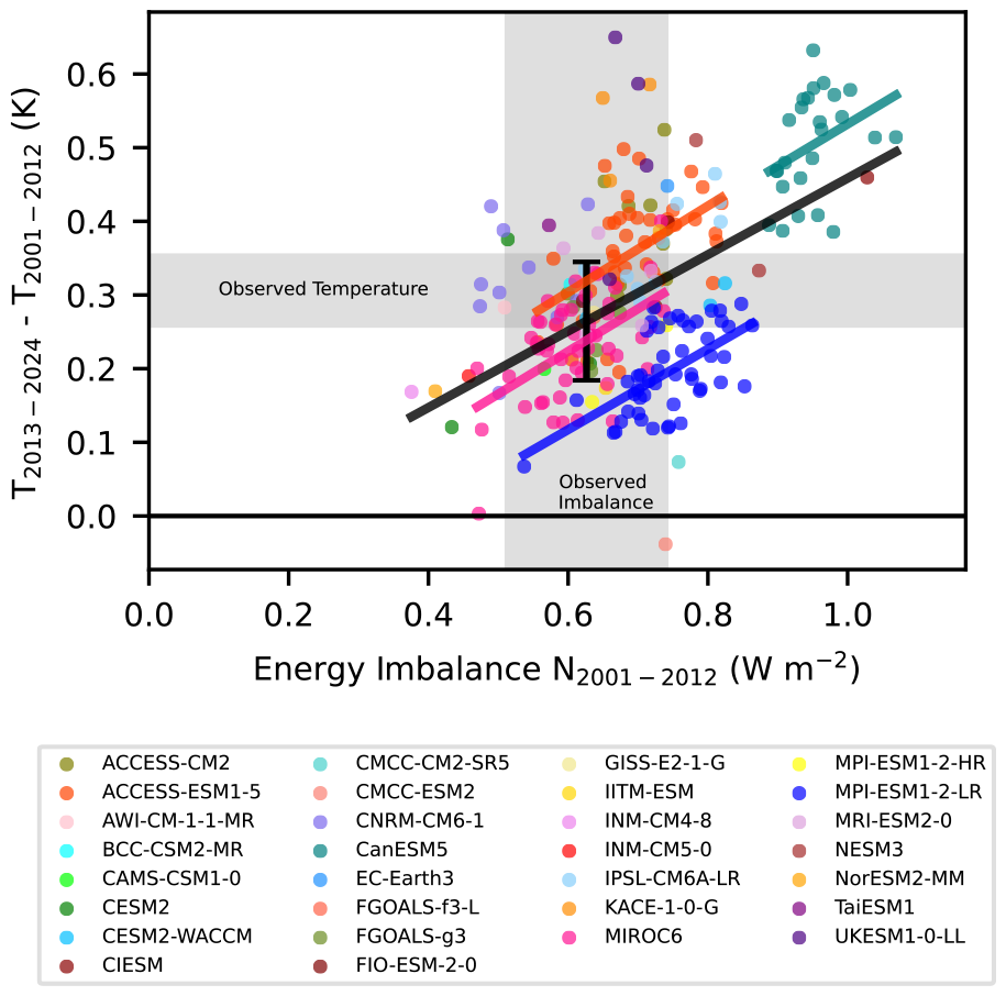
Figure 10 Scatter plot of mean energy imbalance 2001–2012 and change in near-surface air temperature from 2001–2012 to 2013–2024 as simulated by CMIP6 models. Linear regressions are shown for individual models (coloured lines) as well as for the multi-model ensemble (black line). The shaded regions show the observed temperature change and energy imbalance. The error bar corresponds to the predicted temperature change as per the emergent constraint between temperature change and energy imbalance.

We find, however, little evidence that models have generally implemented volcanic aerosols in the scenario according to protocol (Figs. 9 and A2). Instead, the majority of models show relatively small discontinuities, and most models actually exhibit positive shifts, which is inconsistent with the idea that the underestimated trend in energy imbalance is caused by too much volcanic aerosols in the future scenario.

Some models do show a negative discontinuity that appears consistent with protocol (Fig. A2). To corroborate this further, we inspect the clear-sky net shortwave and longwave fluxes (Figs. A3 and A4), here defined as positive downwards to be consistent with their impact on the energy imbalance. We do find negative shifts also in the clear-sky net shortwave radiation in CESM2, CESM2-WACCM, CMCC-CM2-SR5, CMCC-ESM2, GISS-E2-1-G, suggesting that these models followed the experimental protocol. Consequently, these models could have shown a larger positive trend in their energy imbalance if they had used more realistic volcanic aerosols after 2015. For example, CESM2 would have had a trend of about 0.34 Wm⁻² per decade over the period 1995–2035, twice as much as the model's average trend, which is more in line with the observed trends.

For the remaining models, there is either no discontinuity, or in some cases even positive shifts in both the energy imbalance and the clear-sky net shortwave radiation. The most pronounced cases of the latter are the IITM-ESM and KACE-1-0-G models. This could suggest that these models do not apply volcanic aerosols in the future scenario. For IITM-ESM this leads to an overall positive trend, despite exhibiting a negative trend in the historical experiment. And for KACE-1-0-G, the discontinuity is likely the reason it appears to be very close to the observed trend (Fig. 6), despite having only weak trends before and after the transition (Figs. 3b and 9v).

Overall, our analysis suggests that the general CMIP6 model underestimation of the observed energy imbalance trend cannot be attributed to the implementation of the volcanic aerosols in the future scenario, since only a handful of models exhibit a negative shift in the clear-sky net shortwave flux around 2014–2015. On the contrary, some models exhibit a positive shift, suggesting that they do not apply volcanic aerosol in the scenario, making the simulated trend in the energy imbalance larger than what it should have been.

5 The relation between the imbalance and short-term and long-term warming

The energy imbalance is directly related to the accumulation of energy in the Earth system, so it is a natural constraint on the current rate of warming. But can it be used to constrain warming in the coming decade, or the long-term global warming? Myhre et al. (2025) found an emergent constraint relationship between the trend in absorbed shortwave radiation and end-of-century warming. Here we take a different approach and instead use the magnitude of the imbalance, based on the physical justification that the total imbalance is the actual energy accumulation rate.

We first focus on short-term decadal warming. We divide the CERES EBAF data from 2001–2024 into two consecutive 12-year periods, using the energy imbalance in the first period as input, and global warming between the first and the second period as the quantity to be predicted (Fig. 10). This approach allows us to verify the resulting emergent constraint against observations, something that is rarely possible in climate research. The fitted regression line to all model runs (black) shows a steep and physically reasonable relationship with an intercept close to zero, such that no imbalance leads to a prediction of no warming. The line also intersects the actual observed imbalance and global warming, and therefore correctly predicts the observed decadal warming.

However, although the multi-model relation successfully predicts the observed global warming, individual model ensembles are far off, with one ensemble member showing global cooling and another showing more than twice as fast warming as observed, both cases with an imbalance within the observed confidence interval.

To investigate this problem further, we take advantage of the four largest single-model ensembles available in CMIP6: ACCESS-ESM1-5, CanESM5, MIROC6 and MPI-ESM1-2-LR. For each of these models we fit a separate regression line in colour (Fig. 10). The slopes are surprisingly close to that of the entire CMIP6 ensemble, and in three of the four cases the regression line intersects the observed imbalance and warming. This includes CanESM5, a high-sensitivity model, even though it has all its ensemble members simulating both more imbalance and warming than observed. Thus, although an outlier with respect to the observations, the model provides useful information for constraining decadal warming. The relationship for MPI-ESM1-2-LR is shifted below the observations, although some of its individual ensemble members matched observations. Figure 9y shows a small upward shift and change in trend for this model, although this does not explain why that model under-predicted the decadal warming. We interpret these results to mean that the skill in predicting decadal global warming arises from internal variability, given that the same slope is found in all single-model ensembles. The idea is that ensemble members that are colder than expected in the first period will show a larger imbalance as the negative feedback term (λΔT_s) in Eq. (1) is small, and that these realisations therefore warm relatively more in the second period as a consequence of the larger first-period imbalance. Nevertheless, some models show offsets that are too large to be purely associated with internal variability. As such the analysis shows that there is great potential to predict decadal-scale global warming based on observations of Earth's energy imbalance, but such efforts are hampered by systematic model issues.

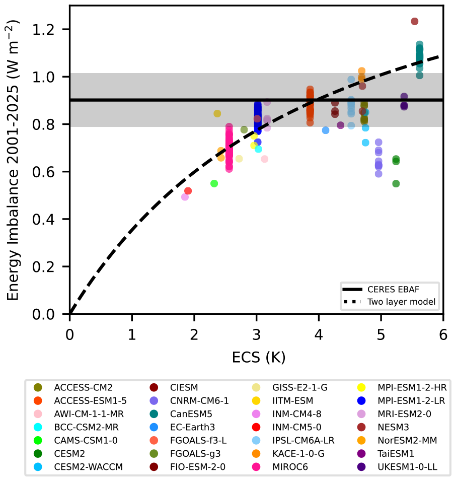
Figure 11 Scatter plot of mean energy imbalance and ECS over the CERES EBAF time period for CMIP6 models (colours) and a two-layer model (black dashed line). CERES EBAF mean energy imbalance (black solid line) along with the 5 %–95 % confidence interval (grey shaded).

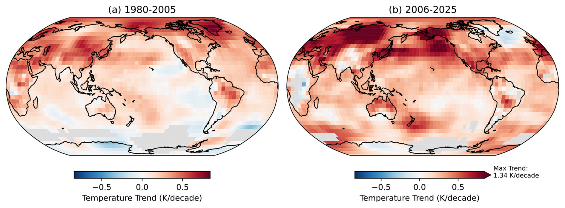
Figure 12 Maps of the near-surface air temperature trend for the periods (a) 1980–2005 and (b) 2006–2025 using the HadCRUT5 observations. Grey shaded areas correspond to regions with at least one missing data point during each period.

Moving focus to long-term warming, we consider the relationship between the current energy imbalance and equilibrium climate sensitivity (ECS $=-F_{\mathrm{2}x}/\mathit{\lambda }$). Here the rationale is that during the ongoing transient warming, if all models apply the same forcing, then models with a large ECS will have a smaller negative λΔT_s despite increased ΔT_s (Hansen et al., 1985), and therefore a larger mean imbalance. The expected relationship is shown by varying only ECS in the two-layer model (Fig. 11). The two-layer model offers an insight into the relationship between ECS and the magnitude of the imbalance, and intersects with observational uncertainties at 3 and 5 K. We see that indeed the vast majority of CMIP6 models closely follow the expected behaviour with low-ECS models showing a low imbalance, and high-ECS models simulating more energy accumulation. The results then favour models with ECS of 3–5 K, and show that some models with lower or higher ECS are less consistent with the observations. Relative to the expected behaviour from the two-layer model, the notable exceptions are the CNRM-CM6-1 and the CESM2 models, and to a lesser extent the CESM2-WACCM model. Inspecting Fig. A2, it is clear that both of the CESM2 model versions show a negative shift in the transition between the historical experiment and the future scenario, and if that had not been the case, both models would have been in line with the energy imbalance simulated by the two-layer model. For the CNRM-CM6-1 ensemble we have not found a viable explanation.

In summary, we find that CMIP6 models in general show only a weak relationship between present-day imbalance and decadal warming, whereas model internal variability shows some skill in predicting short-term warming. A surprisingly close relationship between present-day energy imbalance and long-term warming as represented by ECS suggests that models with moderate climate sensitivity are more realistic.

6 Conclusions

In this study we have investigated the ability of climate models to simulate the magnitude and trend of the energy imbalance at the top-of-atmosphere, while accounting for model energy leakage and remnant drift. We find that climate models exhibit a robust agreement with the observed magnitude of the energy imbalance (5 %–95 % confidence), and that the observed individual annual mean imbalance is within the range simulated by models over the complete time series, including the extreme year 2023.

Regarding the trend, and in line with several recent studies (Raghuraman et al., 2021; Hodnebrog et al., 2024; Myhre et al., 2025), we find that most models underestimate the trend of the energy imbalance in relation to observations. Extending the analysis using the DEEP-C data we also show that this underestimation becomes more pronounced in the most recent decade. That said, despite the general underestimation, a subset of the CMIP6 models do simulate trends that are consistent with observations: Either the simulated trends with internal variability are consistent with the observed trend, or the simulated trends are within the observational uncertainty.

A particular concern we had was that the introduction of the historical mean volcanic aerosol forcing in the future scenario, as recommended by the CMIP6 experiment protocol, could have caused a low bias in the simulated energy imbalance trend since no major volcanoes erupted after 2014. Although we find evidence that a few models could have done this in a negative discontinuity of the clear-sky shortwave radiation between 2014–2015, this does not appear to be a general issue, and some models even show the opposite behaviour. Efforts to simulate the top-of-atmosphere energy imbalance on a more continuous basis could help studies like this in the future (Schmidt et al., 2023).

Finally, we investigated whether the energy imbalance can be used to constrain short-term and long-term global warming. For short-term decadal warming, models show a weak relationship with present imbalance, but internal variability from single-model ensembles does show some potential skill in predicting short-term warming. We do, however, find a surprisingly close relationship between present-day imbalance and equilibrium climate sensitivity, which suggests that models with climate sensitivities of 3 to 5 K best simulate the observed CERES EBAF mean imbalance for 2001–2025.

Stepping back, based on the results presented here we cannot clearly distinguish whether the generally underestimated trend is due to incorrect model forcing feedbacks or an expression of internal variability. Aerosol cooling is decreasing faster than what is simulated in CMIP6 models, due to declining anthropogenic emissions (Hodnebrog et al., 2024), which could help explain the overall underestimated trend in the energy imbalance and hence also the magnitude in recent years. Nevertheless, the fact that models do simulate the magnitude of the imbalance, first above and then below the observations, favours internal variability or incorrectly applied forcing, over an underestimated climate sensitivity. To be more concrete: During the early 2000s the Pacific was dominated by La Niña conditions that caused an unusual warming pattern (Fig. 12). During 1980–2005 the East Pacific ocean shows delayed warming or cooling (Fig. 12a) associated with increased low-level cloudiness, which has a dampening effect on the Earth's energy imbalance by reflecting sunlight (Zhou et al., 2016). Subsequently, the Pacific exhibits alternating El Niño and La Niña conditions, alongside more warming in the East Pacific (Fig. 12b), which could have contributed to the upward trend in absorbed shortwave radiation. Certainly, future studies should be able to bring more clarity on the actual cause of the trend with more data in the coming years.

Appendix A

Table A1 CMIP6 models and number of ensemble members used. Following the official CMIP6 data record we include realizations (r=1 to 50) according to availability, initialisation (i=1), physics (p=1) and forcing (f=1), while for UKESM1-0-LL and CNRM-CM6-1 we used f=2.

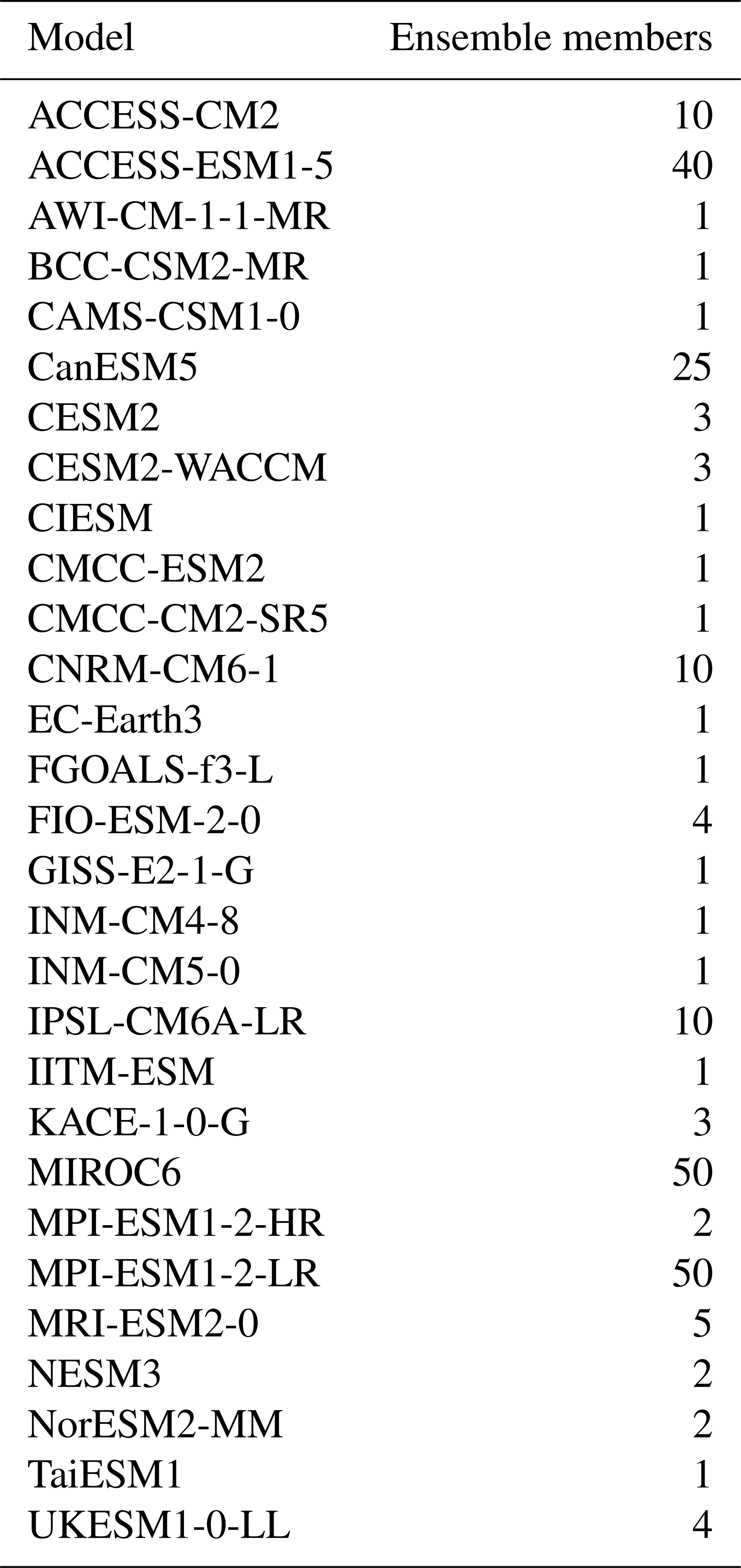
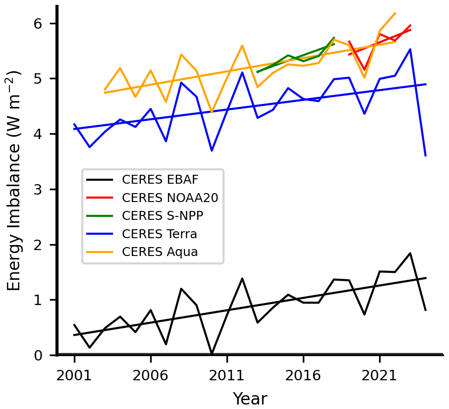
Figure A1 Annual time series of Earth's energy imbalance from the CERES EBAF and several SSF (single-satellite footprint) data products.

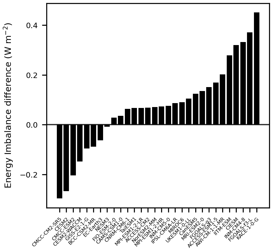
Figure A2 Bar plot of the energy imbalance difference between historical experiment in 2014 and SSP2-4.5 future scenario in 2015 for CMIP6 models.

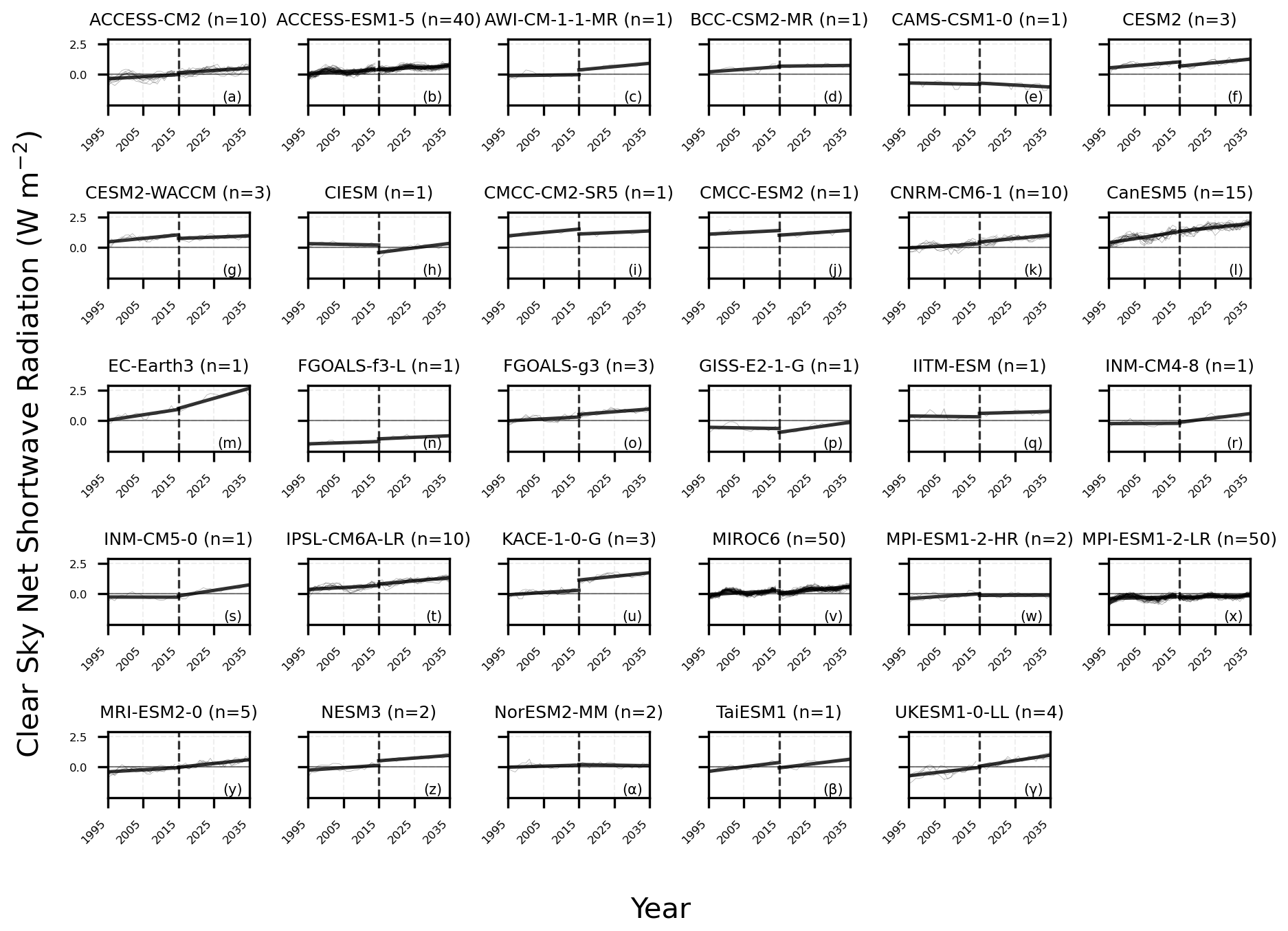
Figure A3 Clear-sky net shortwave radiation time series (grey) and linear fit (black) for historical experiment 1995-2014 and SSP2-4.5 scenario 2015–2035.

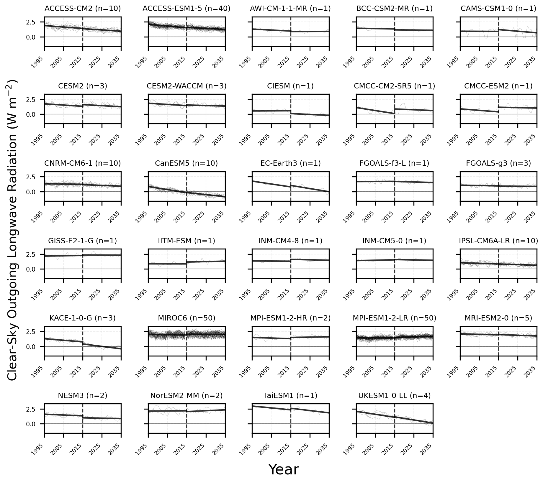
Figure A4 Clear-sky outgoing longwave radiation time series (grey) and linear fit (black) for historical experiment 1995–2014 and SSP2-4.5 scenario 2015–2035.