Large impact of extreme precipitation on projected blue–green water partitioning

Precipitation partitioning into blue (runoff) and green water (transpiration) flows is a fundamental hydroecological process shaping freshwater availability across vegetated and hydrologically active land areas. This partitioning is determined by interactions among climatic conditions, land surface characteristics, and vegetation dynamics, which change with rising temperatures and CO₂ concentrations. Yet, future global shifts in blue–green water partitioning, their controlling factors, and their broader implications remain uncertain. We address this knowledge gap using Earth system model simulations and define the Blue–Green Water Share (BGWS) metric to quantify changes in the relative partitioning of precipitation into runoff and transpiration. Here, we show that projected BGWS changes are spatially heterogeneous rather than dominated by a uniform global shift. Increases in extreme five-day precipitation are most strongly associated with these changes, favouring larger blue water shares. This effect is independent of mean precipitation increases and occurs under both drying and wetting conditions. Additionally, increases in leaf area index tend to favour larger green water shares and counteract the blueward influence of stronger precipitation extremes. Our results provide a process-based perspective on projected blue–green water partitioning and its hydroecological implications.

1 Introduction

Ongoing anthropogenic climate change and other human interventions are reshaping the terrestrial water cycle and altering water availability globally (Wada et al., 2011; Greve et al., 2014; Milly and Dunne, 2016; Wada et al., 2016). These changes affect not only how much precipitation reaches the land surface, but also how that precipitation is partitioned among terrestrial water pathways. This matters because the same amount of precipitation can be divided into different shares of runoff, soil moisture, evaporation, and transpiration. This partitioning affects water availability in rivers, reservoirs, and aquifers, as well as ecosystems and land–atmosphere interactions (Falkenmark, 2013; Falkenmark et al., 2019; Gleeson et al., 2020). Observations and Earth system models (ESMs) show that major land-water fluxes and stores are already changing in their amount, timing, and spatial distribution (Yang et al., 2023; Zaitchik et al., 2023; Gudmundsson et al., 2026). Understanding future water availability therefore requires understanding not only changes in precipitation itself, but also changes in how precipitation is partitioned at the land surface.

To interpret precipitation partitioning in terms of its relevance for ecosystems and human water use, we use the blue–green water paradigm (Falkenmark, 1995; Falkenmark and Rockström, 2006). In this framework, blue water stores refer to water stored in lakes, reservoirs, and aquifers, while blue water flows include runoff; together, these stores and flows support drinking water supply, irrigation, industrial use, and freshwater ecosystems (Falkenmark et al., 2019; Gleeson et al., 2020). Green water stores refer to soil moisture in the unsaturated zone, which supports vegetation growth and terrestrial productivity and is returned to the atmosphere through green water flows, including transpiration and evaporation (Rockström and Gordon, 2001; Falkenmark et al., 2019; Gleeson et al., 2020). Because blue and green water describe different forms and pathways of water availability, this framework complements standard variable-based hydrology by linking hydrological partitioning to its different roles for ecosystems and human water use.

We refer to the partitioning of precipitation into runoff and transpiration as blue–green water partitioning. Focusing on transpiration is useful because it is the vegetation-mediated green water flow through which plants couple water loss to carbon uptake and water-use efficiency (Swann et al., 2016; Nelson et al., 2020). Changes in transpiration are therefore relevant for interpreting vegetation productivity and plant water-use responses to soil-water limitation and atmospheric demand, as well as plant-mediated evaporative cooling and land–atmosphere exchange (Lawrence et al., 2007). By contrast, metrics based on evapotranspiration (ET) or the complement of the runoff coefficient (1−RC) describe broader water-loss or non-runoff signals and can respond differently to climate and vegetation change (Lawrence et al., 2007; Denissen et al., 2022; Bouaziz et al., 2022). Better understanding how precipitation is partitioned between runoff and transpiration is therefore important for interpreting shifts between runoff-related blue water availability and vegetation-mediated green water use.

Under climate change, this blue–green water partitioning is expected to shift because the climatic and hydroecological controls on runoff and transpiration are changing at the same time. Rising CO₂ can reduce stomatal conductance and alter plant water-use efficiency (WUE), while changes in vegetation biomass can modify terrestrial water use and runoff responses (Leakey et al., 2009; Swann et al., 2016; Ukkola et al., 2016; Zhu et al., 2016; Mankin et al., 2018). At the same time, changes in atmospheric demand, soil moisture, and precipitation characteristics, including rainfall intensity and seasonality, can alter the balance between infiltration, storage, runoff generation, and transpiration (Donat et al., 2016; Skinner et al., 2017; Yin et al., 2018; Tabari, 2020; Scheff et al., 2022). Future changes in blue–green water partitioning therefore reflect interacting changes in climate and vegetation rather than changes in precipitation alone.

A growing body of work has already examined related aspects of precipitation partitioning. Studies of drought and climate change show that runoff and ET or transpiration can respond differently, with blue water flows in some regions declining more strongly than green water flows (Ukkola et al., 2016; Orth and Destouni, 2018). ESM analyses further show that vegetation change can reduce runoff across large parts of vegetated land, including in regions where precipitation increases (Mankin et al., 2018, 2019). Other studies have analysed related forms of terrestrial water partitioning at regional to global scales and highlighted the roles of hydrologic setting, catchment characteristics, rainfall intensity, land-surface processes and land use in shaping how precipitation is divided between runoff, storage, and ecosystem water use (Weiskel et al., 2014; Eekhout et al., 2018; Yang et al., 2018; Scheff et al., 2022; Althoff and Destouni, 2023). Together, these studies have improved understanding of individual water fluxes, specific processes, and regional partitioning behaviour. However, less is known about the projected global patterns of runoff–transpiration partitioning across vegetated land areas and the factors associated with the spatial patterns of these changes.

This study aims to assess where future changes favour blue or green water pathways and which climatic and hydroecological changes are associated with these shifts. To do so, we define the Blue–Green Water Share (BGWS), a metric that quantifies the relative partitioning of precipitation into runoff and transpiration. We analyse the historical distribution of BGWS (1985–2014) and its projected changes under the SSP3–7.0 scenario (2071–2100 minus 1985–2014) using an ensemble of 12 ESMs participating in the Coupled Model Intercomparison Project Phase 6 (CMIP6; Eyring et al., 2016; Table S1). We then relate changes in BGWS to changes in mean and extreme precipitation, atmospheric water demand and cloud cover, soil moisture, and vegetation properties. Finally, we examine how BGWS changes co-occur with absolute changes in runoff and transpiration to provide a process-based interpretation of future changes in blue and green water availability and to discuss their implications in a warming, CO₂-enriched world.

2 Data and methods

2.1 Earth system model data

We use output from 12 CMIP6 ESMs for both the historical experiment and the SSP3-7.0 scenario (Eyring et al., 2016; Table S1). SSP3-7.0 represents a regional rivalry pathway (Shared Socioeconomic Pathway 3) with a radiative forcing of 7 W m⁻² by 2100 (Representative Concentration Pathway 7.0; Fujimori et al., 2017; Riahi et al., 2017). We select SSP3-7.0 because the warmest scenario, SSP5-8.5, is unlikely to be realised under current and projected emission trajectories (Hausfather and Peters, 2020). SSP3-7.0, as the second-highest emission scenario, is therefore particularly relevant for current climate impact assessments. However, we acknowledge that hydroecological responses are scenario-dependent (Yang et al., 2018). Given the impact focus of our analysis, we prioritise a scenario whose coupled forcings are more directly policy-relevant outcomes than idealised experiments.

The ESMs are selected to provide the variables required to compute the BGWS metric (Sect. 2.4) and the climatic and hydroecological variables used in the subsequent analyses (Sect. 2.5). Additionally, only models with time-varying leaf area index (LAI) were considered (Table S1). For each model, we select the ensemble member with the lowest available indices along the CMIP6 ensemble axes (“ripf”: realisation, initialisation, physics and forcing; member IDs in Table S1). This approach ensures that each model contributes equally to the analysis and avoids over-representing models with a larger number of ensemble members.

2.2 Observation-based and reanalysis datasets

To evaluate the performance of the selected CMIP6 models in representing the BGWS, we compare the ESM results against observation-based and reanalysis datasets. Specifically, we compute the BGWS from GPCC precipitation (Schneider et al., 2022), G-RUN runoff (Ghiggi et al., 2019), and GLEAM transpiration (Miralles et al., 2011), providing an observation-based reference for model evaluation. These datasets are derived using different methodologies: GPCC is a gauge-based precipitation dataset, G-RUN reconstructs global runoff using a machine-learning approach trained on streamflow observations, and GLEAM is a hybrid observation–model product that estimates land-surface evaporation and transpiration from satellite-based data. Thus, these reference datasets are not equally direct observations and, due to their independent origins, are not fully consistent with one another or with a closed global water balance (Huang et al., 2026). To account for this, we also use ERA5-Land, a physically consistent reanalysis dataset providing all required variables from a single modelling framework (Muñoz-Sabater et al., 2021). However, reanalysis data are not direct observations and inherit uncertainties from model physics, model parametrisations and input data quality. While ERA5-Land offers a spatially and temporally coherent dataset, its ability to accurately represent long-term hydrological changes remains uncertain (Dutta and Markonis, 2024). We therefore use these global-scale gridded datasets as a first-order consistency check of ESM simulated BGWS patterns, rather than as a full benchmarking of ESM skill. In addition to comparing climatological BGWS fields, we also assess whether the ensemble mean reproduces observed changes in BGWS over the recent historical period. For this purpose, we compare BGWS changes between 1985–1999 and 2000–2014 in the CMIP6 ensemble mean and the reference datasets.

2.3 Data preprocessing and multi-model ensemble

To enable spatial comparison across models and datasets, we regrid all fields to a common 1°×1° latitude–longitude grid using conservative interpolation. After regridding, we compute 30-year climatological means for a historical period (1985–2014) and a far-future period (2071–2100). Future-minus-historical changes are then calculated for all variables used in the subsequent analyses.

We apply a fixed historical mask derived from the ensemble mean over 1985–2014. The Greenland/Iceland and Antarctic regions are excluded a priori using the reference regions of the Sixth Assessment Report of the Intergovernmental Panel on Climate Change (IPCC AR6; Iturbide et al., 2020), because they are dominated by permanent ice cover and fall outside the vegetated runoff–transpiration domain targeted here. The mask restricts the remaining analysis to vegetated and hydrologically active land areas where the subsequent runoff–transpiration partitioning analysis is meaningful. Grid cells are retained only where mean precipitation exceeds 0.822 mm d⁻¹ (≈ 300 mm yr⁻¹) and where both mean runoff and mean transpiration exceed 0.05 mm d⁻¹. These values are conservative screening thresholds rather than hydroclimatic regime definitions. They exclude grid cells with low water input or negligible runoff or transpiration, where a runoff–transpiration partitioning interpretation is less robust.

The precipitation threshold follows the order of magnitude used in the IPCC description of arid zones (IPCC, 2022), and the runoff threshold matches the value used to mask very low-runoff grid cells in a comparable large-scale impact assessment (Schleussner et al., 2016). We apply the same low-flux threshold to transpiration because both fluxes enter the BGWS metric directly and symmetrically. Because non-negligible transpiration requires active vegetation, these criteria also exclude bare and sparsely vegetated land. The same mask is applied consistently to all historical fields, future changes, and reference datasets. It is also applied identically to all 12 ESMs, so that ensemble statistics and individual-model attributions are evaluated on the same spatial domain.

We employ an unweighted multi-model ensemble (hereafter referred to as the ensemble mean) to mitigate uncertainties associated with individual model biases and initial-condition variability. For each model, climatological means and changes are first computed at the model level and then averaged across models to obtain the ensemble mean. This ordering ensures that ensemble statistics reflect individual model responses before averaging. We do not apply performance-based weighting, as our objective is to assess broad climate impacts rather than to optimise the ensemble for a specific variable. Spatial means are always calculated as area-weighted averages to account for the convergence of meridians with latitude. Each grid cell is weighted by the cosine of its latitude, cos (φ), where φ denotes latitude.

2.4 Blue–Green Water Share

In this study, we analyse blue–green water partitioning using precipitation (P; mm d⁻¹) as the incoming water supply, runoff (R; mm d⁻¹) as blue water flow and transpiration (E_t; mm d⁻¹) as the vegetation-mediated green water flow in vegetated and hydrologically active land areas. We focus on transpiration because it represents the direct vegetation water-use response, whereas non-transpiration evaporation may respond differently to climate change than vegetation-mediated water use (Lawrence et al., 2007). This distinction matters because total ET can reflect offsetting changes in its components. For example, transpiration can decrease while soil evaporation increases, so the ET response emerges from opposing biological and physical processes (Berg and Sheffield, 2019). Using ET instead of transpiration would therefore address a different question, namely runoff versus total evaporative loss rather than runoff versus vegetation-mediated water use (Denissen et al., 2022).

We introduce BGWS as a flow-based partitioning metric for runoff and transpiration rather than as a complete representation of all blue and green water or water-balance components. BGWS thus does not represent total green water flow, but specifically the vegetation-mediated component of green water use captured by transpiration. The historical mask defined in Sect. 2.3 ensures that the metric is evaluated only in regions where this transpiration-based interpretation is meaningful.

We define the BGWS metric as:

$$\begin{array}{}\text{(1)}& \text{BGWS}={\displaystyle \frac{R-E_{\mathrm{t}}}{P}}\times \mathrm{100},\end{array}$$

which is dimensionless and expressed in percent. Positive BGWS values indicate that a larger share of precipitation is partitioned towards runoff, whereas negative BGWS values indicate that a larger share is partitioned towards transpiration.

BGWS is therefore complementary to existing partitioning metrics. Relative to the blue water trade-off (BWT) metric used by Mankin et al. (2018, 2019), BGWS contrasts runoff directly with transpiration, does not include interception or storage terms, and reports the result as a normalised share of precipitation. Thus, interception-driven canopy effects are not represented explicitly by BGWS. For assessing vegetation-mediated green water use, however, transpiration as a direct ESM output is useful because it provides an immediate indicator of plant water use.

We focus on water fluxes rather than water stores because hydrological fluxes are more consistently available and more directly comparable across the selected CMIP6 ESMs. Moreover, on multi-decadal timescales (here, 30-year means), storage changes tend to be small relative to fluxes, as many catchments approach a near-steady state within this period (Han et al., 2020). Neglecting storage terms therefore provides a pragmatic and interpretable framework for large-scale analysis, although this simplification remains a limitation and an avenue for future research.

Changes in BGWS, denoted as ΔBGWS, indicate shifts in blue–green water partitioning and are calculated as

$$\begin{array}{}\text{(2)}& \mathrm{\Delta }\text{BGWS}={\text{BGWS}}_{\text{Future}}-{\text{BGWS}}_{\text{Historical}}.\end{array}$$

A positive ΔBGWS reflects an increasing partitioning towards blue water flow, whereas a negative ΔBGWS indicates an increasing partitioning towards green water flow. Although ΔBGWS does not directly measure absolute changes in all blue and green water components, it provides a clear measure of the changing trade-off between runoff and transpiration.

To complement the transpiration-based analysis, we also compute non-transpiration evaporation E_nt as the difference between ET and transpiration E_t,

$$\begin{array}{}\text{(3)}& E_{\mathrm{nt}}=\text{ET}-E_{\mathrm{t}}.\end{array}$$

This quantity represents non-transpiration evaporation, including soil evaporation, interception evaporation, and other non-transpiration components as represented in each dataset. We do not use CMIP6 component evaporation variables directly because key components (e.g. evspsblsoi) are unavailable for many models.

2.5 Climatic and hydroecological variables

We analyse both the historical 30-year climatological means and the future-minus-historical changes in selected climatic and hydroecological variables associated with the distribution and shifts in blue–green water partitioning. The selected variables are mean precipitation (P; mm d⁻¹), precipitation seasonality (P_seas; mm d⁻¹), annual maximum consecutive five-day precipitation (RX5day; mm), surface soil moisture (SM_surf; mm), leaf area index (LAI; m² m⁻²), transpiration-based water-use efficiency (WUE; $\mathrm{gC}{\mathrm{m}}^{-\mathrm{2}}{\mathrm{mm}}^{-\mathrm{1}}$), mean vapour pressure deficit (VPD; hPa), VPD seasonality (VPD_seas; hPa), and total cloud cover (CLT; %). Except for RX5day, which is derived from daily precipitation, all variables are based on monthly mean output. The variable selection is based on the predictor screening described in Sect. 2.6. Seasonality, RX5day, VPD, and WUE are computed as follows.

Precipitation and VPD seasonality are defined as the standard deviation of the 12 monthly climatological means within each 30-year period. For a given variable X and monthly climatology ${\stackrel{\mathrm{‾}}{X}}_m$, seasonality is computed as

$$\begin{array}{}\text{(4)}& X_{\mathrm{seas}}=\sqrt{{\displaystyle \frac{\mathrm{1}}{\mathrm{12}}}\sum _{m=\mathrm{1}}^{\mathrm{12}}{\left({\stackrel{\mathrm{‾}}{X}}_m-\stackrel{\mathrm{‾}}{X}\right)}^{\mathrm{2}}},\end{array}$$

where ${\stackrel{\mathrm{‾}}{X}}_m$ is the climatological mean for month m and $\stackrel{\mathrm{‾}}{X}$ is the mean of the 12 monthly climatological values.

RX5day is derived from daily precipitation as the annual maximum consecutive five-day precipitation. For a given year j,

$$\begin{array}{}\text{(5)}& {\text{RX5day}}_j=max\left(R{R}_{kj}\right),\end{array}$$

where RR_kj denotes total precipitation accumulated over any five-day interval ending on day k within year j. For each 30-year period, RX5day is averaged over the annual maxima.

VPD is calculated using the Buck equation (Buck, 1981) to estimate saturation vapour pressure (e_s),

$$\begin{array}{}\text{(6)}& e_{\text{s}}=\mathrm{611.21}\times \exp \left[\left(\mathrm{18.678}-{\displaystyle \frac{T}{\mathrm{234.5}}}\right)\left({\displaystyle \frac{T}{\mathrm{257.14}+T}}\right)\right],\end{array}$$

where T is near-surface air temperature in °C, and 611.21 Pa is the saturation vapour pressure at 0 °C. Actual vapour pressure (e_a) is obtained from specific humidity (q) and surface pressure (p_s, in Pa) as

$$\begin{array}{}\text{(7)}& e_{\text{a}}={\displaystyle \frac{q{p}_{\text{s}}}{\mathrm{0.622}+\mathrm{0.378}q}},\end{array}$$

and VPD is then given by

$$\begin{array}{}\text{(8)}& \text{VPD}=e_{\text{s}}-e_{\text{a}}.\end{array}$$

VPD is converted from Pa to hPa for the analysis.

We use the ratio of gross primary productivity (GPP) to transpiration to compute WUE, a widely used proxy for the CO₂ effect on stomatal resistance (Keenan et al., 2013; Lian et al., 2021; Ruehr et al., 2023):

$$\begin{array}{}\text{(9)}& \text{WUE}={\displaystyle \frac{\text{GPP}}{E_{\text{t}}}},\end{array}$$

which quantifies the efficiency of carbon assimilation per unit of water consumed by vegetation through transpiration.

2.6 Multiple regression analysis

We construct multiple linear regression (MLR) models with Elastic Net regularisation separately for the two historical BGWS regimes to explain the spatial pattern of projected ΔBGWS across grid cells. Each grid cell is treated as one sample, and both the predictors and the response variable are based on ensemble mean changes between the future and historical periods. The analysis therefore explains spatial differences in projected ΔBGWS within each regime. It does not attribute the temporal evolution of BGWS at individual grid cells or regions.

Because neighbouring grid cells are not independent, we apply spatially blocked cross-validation. Grid cells are grouped into 10°×20° latitude–longitude blocks, and all model training, tuning, and testing are performed using these spatial blocks as groups. For each regime, we apply repeated grouped train–test splits with 20 % of the spatial blocks held out per repeat, combined with nested grouped cross-validation for Elastic Net hyperparameter tuning. To favour simpler models and reduce overfitting, the final hyperparameters are selected using a one-standard-error rule. Model performance is evaluated using out-of-sample R² on held-out spatial blocks.

To address multicollinearity among predictors and to regularise the regression, we apply Elastic Net regularisation (Friedman et al., 2010). The Elastic Net objective function is

$$\begin{array}{}\text{(10)}& \underset{\mathit{\beta }}{min}\left[{\displaystyle \frac{\mathrm{1}}{\mathrm{2}n}}\sum _{i=\mathrm{1}}^n(y_i-{\widehat{y}}_i{)}^{\mathrm{2}}+\mathit{\alpha }\mathit{\rho }\sum _{j=\mathrm{1}}^p|{\mathit{\beta }}_j|+{\displaystyle \frac{\mathit{\alpha }(\mathrm{1}-\mathit{\rho })}{\mathrm{2}}}\sum _{j=\mathrm{1}}^p{\mathit{\beta }}_j^{\mathrm{2}}\right],\end{array}$$

where y_i and ${\widehat{y}}_i$ are the observed and predicted values, n is the number of samples, β_j are the regression coefficients, α controls the overall regularisation strength, and ρ determines the balance between L1 (Lasso) and L2 (Ridge) penalties. The L1 penalty promotes sparsity by shrinking some coefficients to exactly zero, whereas the L2 penalty shrinks coefficients towards zero without eliminating them, helping to stabilise estimates under multicollinearity. Prior to model fitting, all predictors are standardised to zero mean and unit variance within each training split, while ΔBGWS is left on its original scale.

The final predictor set was selected from a larger initial set of candidate predictors according to their contribution to predictive performance, their physical interpretability, and data availability across the full 12-model ensemble (Sect. S2). The final set includes changes in mean precipitation, precipitation seasonality, RX5day, mean VPD, VPD seasonality, total cloud cover, near-surface soil moisture, LAI, and WUE. Together, these variables represent climatic and hydroecological processes relevant to climate change impacts and allow physical interpretation of their influence on ΔBGWS. Changes in mean precipitation, precipitation seasonality, and extreme precipitation represent water supply and hydrological extremes. RX5day is used as the main extreme precipitation metric because multi-day precipitation accumulation shows slightly better spatial agreement than single-day extremes in CMIP6 and observational evaluations, making it a more robust indicator of extreme precipitation in large-scale datasets (Li et al., 2021a; Dunn et al., 2022). Changes in mean vapour pressure deficit and VPD seasonality represent atmospheric dryness and plant water stress. Changes in near-surface soil moisture represent surface water availability, while changes in LAI and WUE represent vegetation state and plant physiological responses to elevated CO₂. Changes in LAI reflect both climatic and human influences, including land-use and land-cover change, although these contributions are not isolated explicitly here. Changes in total cloud cover represent an additional atmospheric control related to energy and moisture conditions.

To quantify the contribution of each predictor to model performance, we compute permutation importance scores (Breiman, 2001). This model-agnostic metric is obtained by randomly permuting the values of a given predictor and quantifying the resulting change in R². For each repeat and each predictor, predictor values are permuted 20 times and the resulting decrease in R² is recorded. We interpret these test-set importance scores as measures of the contribution of each predictor to the spatial pattern of projected ΔBGWS within each regime. For comparison with the ensemble-mean attribution, we repeat the same blocked regression workflow for each individual ESM and report individual-model permutation importances only where mean held-out R²>0.3.

3 Results and discussion

3.1 Historical distribution of BGWS

The historical BGWS pattern in the CMIP6 ensemble mean (1985–2014; Fig. 1a) reveals three overarching features: energy-limited, water-limited, and precipitation-seasonality regulated blue–green water partitioning. The first two features are consistent with the broader literature distinguishing energy- and water-limited land-surface or ecosystem regimes, while the third extends this logic to precipitation-seasonality effects that are particularly relevant for blue–green water partitioning (Seneviratne et al., 2010; Denissen et al., 2022). On average, the area-weighted BGWS is slightly positive, indicating that ∼3 % more precipitation is partitioned towards blue water flow, with notable ensemble variability from −13 % to +17 % (Table S4). These contrasts stem from differences in the model representation of precipitation characteristics, land-surface hydrology, and vegetation dynamics, which contribute to well-documented CMIP6 biases in simulated land-surface water fluxes relative to reference products (Clark et al., 2015; Gentine et al., 2019; Zheng et al., 2019; Li et al., 2021b; Padrón et al., 2022; Yang et al., 2023).

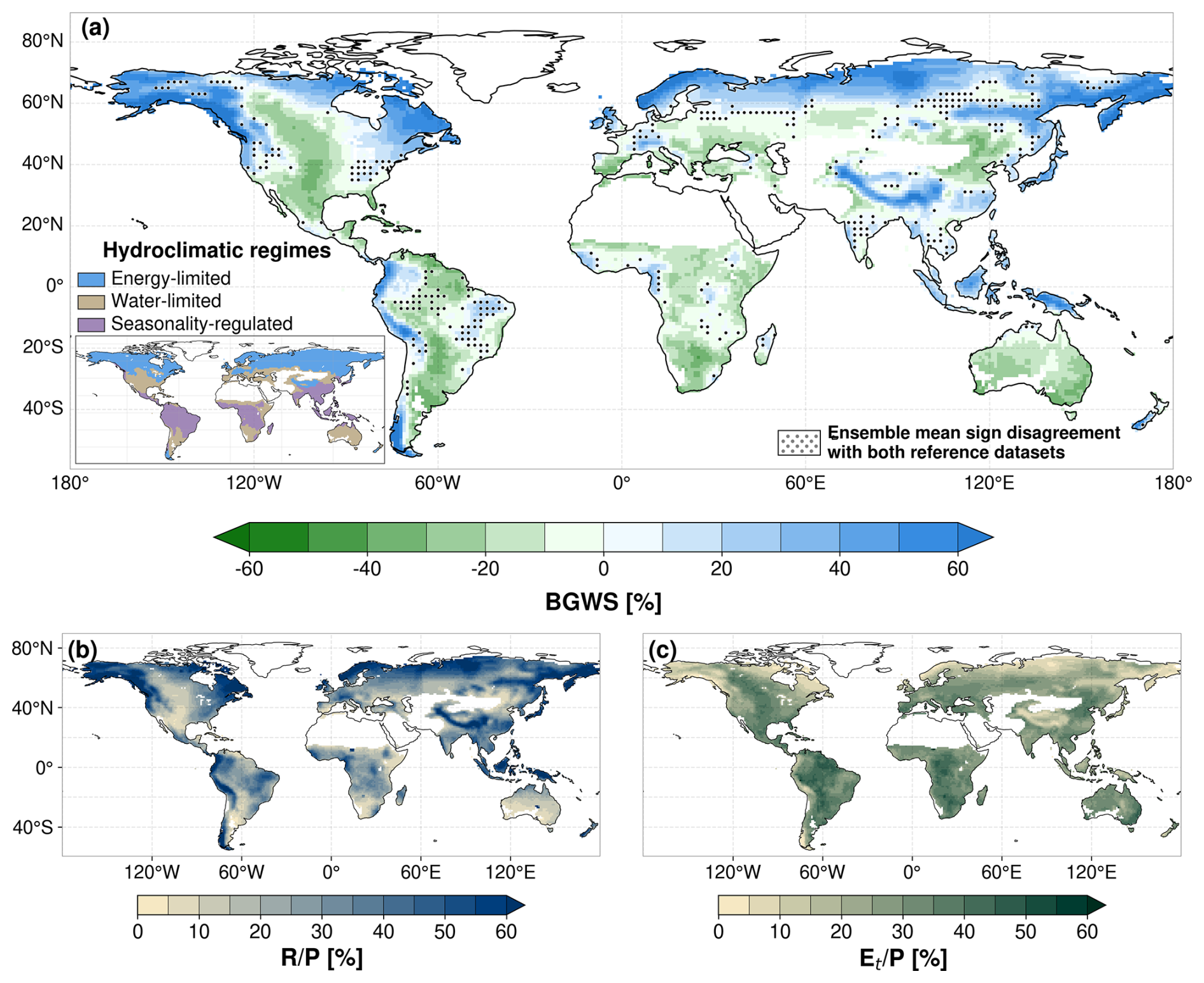
Figure 1 Ensemble mean for the historical period (1985–2014) based on 12 CMIP6 Earth system models. (a) BGWS [%] with inset showing a simple hydroclimatic regime classification in which each grid cell is assigned to the regime with the strongest standardized signal of low near-surface soil moisture, low air temperature, or high precipitation seasonality. (b) runoff share, $R/P$ [%], and (c) transpiration share, $E_{\mathrm{t}}/P$ [%]. Blue colours in the BGWS colour map indicate a greater partitioning of precipitation towards runoff (blue water flow), whereas green colours indicate a greater partitioning towards transpiration (green water flow). All panels use the fixed historical analysis mask described in Sect. 2.3. Stippling in panel (a) indicates regions where the sign of the ensemble mean BGWS disagrees with both reference datasets.

Comparing the spatial pattern of the ensemble mean BGWS with observation-based and reanalysis products indicates a reasonable large-scale representation for the historical climatology (Fig. S2). Agreement is weaker, but still qualitatively similar, for recent historical changes over the shorter evaluation period (Fig. S3). Compared with both reference datasets, the ensemble mean BGWS values are biased towards too much blue water. Decomposing BGWS into runoff ($R/P$) and transpiration ($E_{\mathrm{t}}/P$) ratios shows that the bias is driven primarily by underestimated $E_{\mathrm{t}}/P$ (negative mean offset), while regional differences in $R/P$ also contribute (Figs. S4 and S5). One possible structural contribution to the underestimated $E_{\mathrm{t}}/P$ bias is the limited representation of lateral groundwater redistribution in many large-scale land models used in ESMs, where this process is often overlooked or strongly simplified. By underrepresenting shallow groundwater support to ET in drylands or during dry periods, this may partly favour a more blue-biased BGWS (Maxwell and Condon, 2016; Liao et al., 2025). Accordingly, we treat BGWS as a process indicator and base interpretation primarily on directional patterns, sign-robust spatial structures, and covariation with relevant predictors, while avoiding detailed interpretation in regions with disagreement against both reference datasets (stippling in Fig. 1a).

Energy-limited blue–green water partitioning, the first BGWS feature, is dominant across higher latitudes (>60° N) and high-altitude regions, which consistently show greater partitioning towards blue water flow (Fig. 1a). This pattern aligns with the Budyko framework, which links energy-limited conditions to increased runoff (Budyko, 1974). In the higher latitudes, 95 % of the land area exhibits a larger blue water share, with an area-weighted mean BGWS of +36 %. Here, low net radiation (light-limited) and low air temperatures (kinetic/phenology-limited) coincide with below-global-average $E_{\mathrm{t}}/P$, while near-surface soil moisture remains comparatively high (Figs. 1c and S6). Consequently, precipitation predominantly contributes to runoff (Fig. 1b). Mountain ranges exhibit similar behaviour, where orographically enhanced precipitation and topography-controlled runoff parametrisations in ESMs (e.g., SIMTOP) can contribute to larger blue water shares (Niu et al., 2005; Gnann et al., 2025). Snowmelt-driven runoff likely further enhances blue water shares in cold regions (Barnett et al., 2005), although simplified representation of snow sublimation in ESMs may also contribute to runoff overestimation in some high-altitude regions and thus reinforce locally blue-biased partitioning (Stigter et al., 2018). Ongoing warming-related snow cover loss, by contrast, increases net radiation and ET and can reduce runoff (Milly and Dunne, 2020). Energy-limited partitioning is also evident across parts of the mid-latitudes (40–60° N/S), but with much smaller positive BGWS values than in the higher latitudes, with an area-weighted mean BGWS of about +6 %. This is consistent with seasonal transitions between winter energy limitation and summer water limitation (Seneviratne et al., 2010; Knoben et al., 2018). Compared with observation- and reanalysis-based products, however, the ensemble mean tends to overstate both the magnitude and the spatial extent of blue water shares in energy-limited high- and mid-latitudes (Fig. S2).

Water-limited blue–green water partitioning, the second BGWS feature, dominates in semi-arid and dry sub-humid regions such as the Eurasian Steppe or Australia’s Outback (Fig. 1a). These water-limited environments are marked by annual precipitation below the global mean and relatively low near-surface soil moisture (Fig. S6). Despite these hydrological constraints, these ecosystems partition a larger fraction of available water towards transpiration, increasing the green water share in line with observation-based data (Figs. 1 and S2). The RX5day-to-annual-precipitation ratio is elevated across many of these dryland regions (Fig. S7), indicating that rainfall is often temporally concentrated even where mean precipitation is low. Nevertheless, within the retained vegetated drylands, the annual partitioning still tends to favour transpiration over runoff. This is consistent with water-limited ecosystems maintaining relatively low runoff fractions while using a large share of the limited incoming precipitation for vegetation water use (Althoff and Destouni, 2023).

Precipitation-seasonality regulated blue–green water partitioning, the third BGWS feature, emerges most clearly in monsoonal and other strongly seasonal climates highlighted by the inset in Fig. 1a. In these regions, BGWS depends not only on how much precipitation falls annually, but also on how strongly rainfall is concentrated within the year. Regions with high precipitation seasonality, such as southern and eastern Asia and parts of the Maritime Continent, tend to show larger blue water shares where wet-season rainfall is strongly concentrated, RX5day is high, and near-surface soil moisture is comparatively high (Figs. 1 and S6). By contrast, humid regions with more weakly seasonal rainfall, such as much of the Amazon and central Africa, tend to show larger green water shares and higher $E_{\mathrm{t}}/P$. Thus, the contrast is not simply between wet and dry regions, but between climates with strongly concentrated wet seasons and those with more even rainfall distribution. This mechanism is also consistent with the contrast between East Asian monsoon regions, which show larger blue water shares, and subtropical regions such as the Florida Peninsula, where more evenly distributed rainfall coincides with larger green water shares.

Overall, the historical BGWS distribution is therefore consistent with a transition from energy-limited blue-water dominance in cold and high-altitude regions, to water-limited green-water dominance in semi-arid regions, and to seasonality-regulated partitioning in monsoonal and humid subtropical climates. Several regions, especially within this third feature, also show disagreement with both reference datasets or elevated ensemble spread, underscoring the challenges ESMs still face in representing humid subtropical and tropical hydroecological dynamics (Fiedler et al., 2020; Padrón et al., 2022; Figs. 1a and S8).

3.2 Projected changes in BGWS

Figure 2a maps the projected BGWS changes (2071–2100 minus 1985–2014) under the regional rivalry scenario (SSP3-7.0), separated by whether grid cells historically belong to the blue or green water regime. The four change classes occupy broadly comparable fractions of the analysed land area. In the historical green water regime, 21.5 % becomes greener and 32.8 % less green; in the historical blue water regime, 21.0 % becomes bluer and 24.7 % less blue. Despite this broad balance in areal coverage, the ensemble-mean global BGWS increases slightly by +1.35 ppts (Table S4), with individual-model global mean changes ranging from −1.86 to +5.1 ppts. Regime shifts are less extensive than the strengthening or weakening of existing regimes, and occur more often from green to blue than from blue to green (7.2 % versus 2.4 % of the analysed land area; Fig. S9). Because BGWS reflects the difference between runoff and transpiration relative to precipitation, a larger blue water share arises wherever runoff changes more positively than transpiration, whereas a larger green water share arises wherever transpiration changes more positively than runoff. The spatial expression of these mechanisms varies strongly across latitude bands and climate regimes (Fig. 2).

Larger blue water shares most directly occur where runoff increases more than transpiration increases. This pattern is evident in wetter parts of the historical blue water regime, for example, in northeastern Eurasia and along the East Asian monsoon belt, where enhanced precipitation coincides with increasing runoff and a strengthening of blue-water dominance (Fig. 2). In these regions, both blue and green water flows increase in absolute terms, but runoff gains are larger, so partitioning shifts further towards blue water. Similar positive BGWS changes are also visible in historically blue-water dominated tropical regions such as large parts of India, where future trends are generally positive and coincide with increased wetting (Fig. 2).

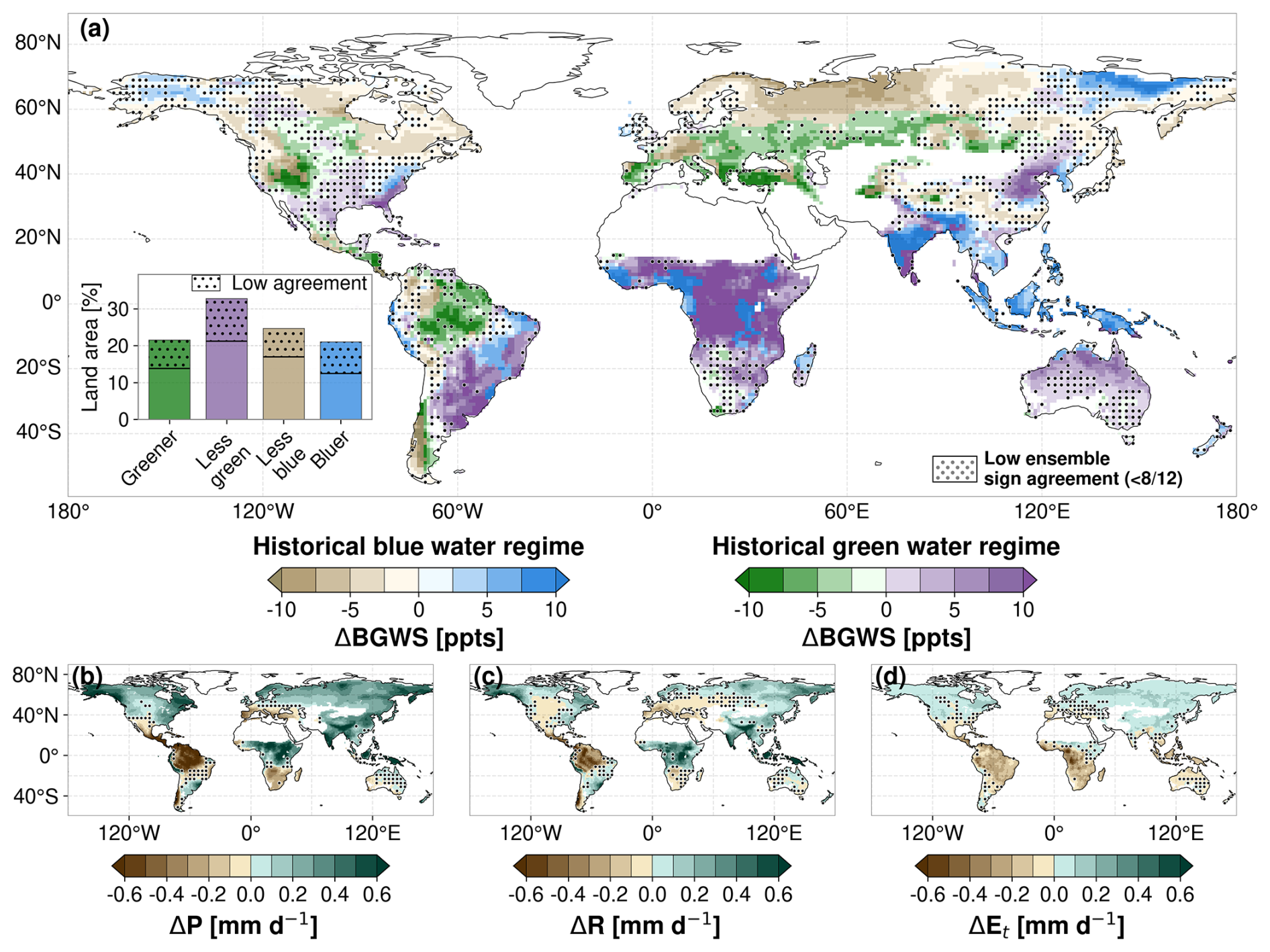
Figure 2 Ensemble mean change (2071–2100 minus 1985–2014) under the SSP3-7.0 scenario based on 12 CMIP6 Earth system models. (a) ΔBGWS [ppts], shown separately for grid cells with historically positive BGWS values (blue water regime; beige to blue colours) and historically negative BGWS values (green water regime; green to purple colours). Blue and purple colours indicate shifts towards larger blue water shares, whereas green and beige colours indicate shifts towards larger green water shares. The inset summarises the analysed land-area fractions of the four BGWS-change classes; bar heights show the total area of each class, the horizontal line marks the fraction with robust sign agreement, and the stippled upper part indicates the fraction with low model agreement. (b) Δ precipitation [mm d⁻¹], (c) Δ runoff [mm d⁻¹], and (d) Δ transpiration [mm d⁻¹]. All panels use the fixed historical analysis mask described in Sect. 2.3. Stippling marks regions of low inter-model agreement, where fewer than 8 of the 12 models agree on the sign of change.

Larger blue water shares can also occur where runoff increases while transpiration decreases. This pattern is especially relevant in parts of the subtropics and tropics, where wetter conditions and increasing runoff coincide with declining transpiration. The major rainforests exhibit an asymmetric response in this respect: only the Amazon rainforest tends towards a greater green water share, whereas parts of central Africa and Maritime Southeast Asia shift towards greater blue water shares. This divergence coincides with precipitation and runoff increases in the latter two regions, while transpiration declines across all three rainforest regions (Fig. 2). Consistent with these regional examples, 69 % of the analysed subtropical land and 77 % of the analysed tropical land are projected to experience larger blue water shares.

A third pathway to larger blue water shares occurs where both runoff and transpiration decrease, but transpiration declines more strongly than runoff. This mechanism is visible in scattered historically water-limited patches of the subtropics and mid-latitudes, for example in parts of eastern Australia and northwestern Mexico (purple in Fig. 2a). In these regions, the relative decline in transpiration exceeds the runoff loss, shifting partitioning towards blue water even though absolute blue water flow may also decline. This contrasts with observed CO₂-driven blue water losses where greening increased ET and reduced streamflow in Australia's sub-humid/semi-arid basins (Ukkola et al., 2016), and with vegetation-driven runoff declines in the American West (Mankin et al., 2017, 2019). While LAI increases across many of these regions, transpiration does not always rise in parallel because higher WUE can offset rising water demands (Figs. 2d and S10). More generally, whether dry regions will experience a blue or green water share increase depends largely on the interplay between rising vegetation water demand and WUE-related transpiration limitations, although structural uncertainties remain in how models represent vegetation responses to rising CO₂ and the resulting water-cycle impacts (Wei et al., 2024; Yang et al., 2021; Forzieri et al., 2020; Yang et al., 2023).

Larger green water shares occur where transpiration increases more than runoff increases. This mechanism is apparent in parts of the higher latitudes and mid-latitudes where leaf area expands and transpiration gains exceed the concurrent runoff increase, for example in northwestern Eurasia (Fig. S10). Consistent with this pattern, 64 % of the analysed land area north of 60° N experiences a decrease in BGWS. Although a larger share of precipitation is partitioned towards green water flow, these regions concurrently experience an increase in blue water flow (Fig. 2c). In such cases, the shift towards green water does not necessarily imply a drying climate, but rather that transpiration becomes relatively more important than runoff.

A larger green water share can also arise where transpiration increases while runoff decreases. This pattern is particularly evident in parts of eastern Europe, where greener partitioning coincides with runoff loss (Fig. 2). In such cases, vegetation gains and enhanced transpiration shift the balance towards green water while blue water availability declines in absolute terms. The same logic applies to other mid-latitude regions where warming- and CO₂-driven vegetation responses amplify transpiration despite weak or negative runoff trends.

Finally, larger green water shares occur where both runoff and transpiration decrease, but runoff declines more strongly than transpiration. This mechanism is evident in parts of southern Europe, where a greater reduction in runoff compared to transpiration results in a green water share increase (Fig. 2). This mechanism is also relevant in other regions with blue water losses, as receiving a smaller or only slightly larger share of precipitation does not offset the overall decline in runoff.

3.3 Climatic and hydroecological predictors of projected BGWS change

The regional BGWS changes described above suggest that future blue–green water partitioning reflects competing effects of changes in mean and extreme precipitation, changes in atmospheric and soil-moisture conditions, and vegetation responses. To quantify which selected predictors best explain the spatial pattern of ΔBGWS within each historical regime, we fitted separate blocked multiple linear regression (MLR) models for the historical blue and green water regimes (Sect. 2.6). Figure 3 summarises the resulting permutation importance scores for the ensemble mean together with the corresponding importance ranks from individual ESMs. The ensemble-mean ranking should be interpreted as the common large-scale signal across the 12-model ensemble field, while the individual ESM points illustrate model-to-model variability in predictor importance. Both MLR models show moderate to strong predictive skill (R²=0.51 for the historical blue water regime and R²=0.74 for the historical green water regime). This interpretation and the importance rankings are further supported by the nonlinear Random Forest sensitivity analysis (Fig. S11).

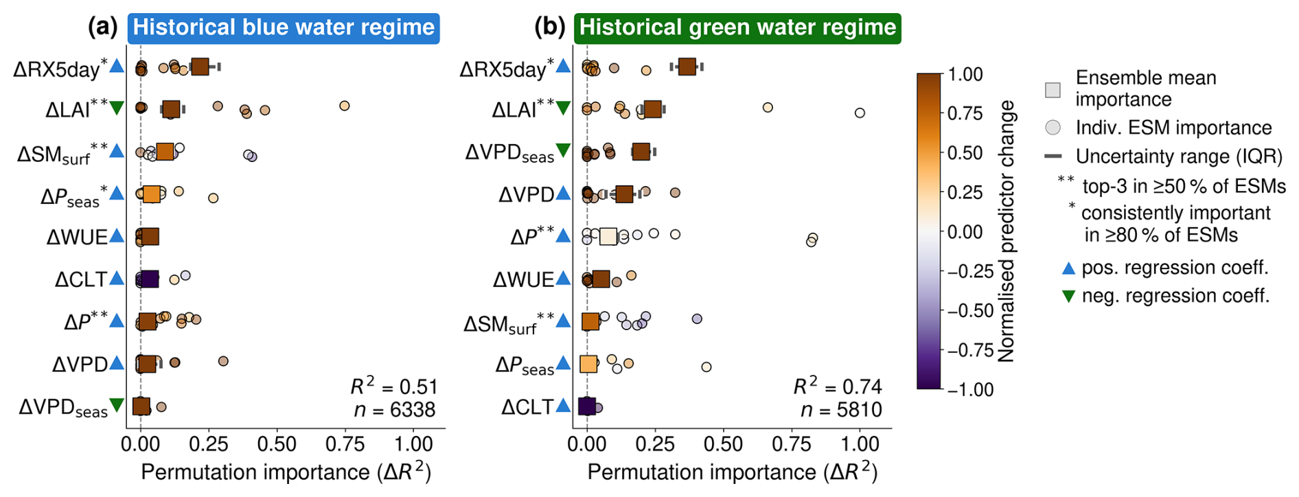
Figure 3 Variable importance for the spatial attribution of projected changes (2071–2100 minus 1985–2014) in ΔBGWS under the SSP3-7.0 scenario in the two historical BGWS regimes shown in Fig. 2: (a) historical blue water regime and (b) historical green water regime. Squares show the median permutation importance (ΔR²) of the 12-model CMIP6 ensemble mean for the predictor set, and horizontal lines show the interquartile range across repeated blocked cross-validation splits. Circles show the median permutation importance from individual ESMs with mean model performance R²>0.3. Colours indicate the normalised mean change of each predictor within the respective regime. Upward blue triangles indicate positive regression coefficients and downward green triangles indicate negative regression coefficients in the ensemble mean. Reported R² values give the mean model performance. The attribution is fitted only for grid cells retained by the fixed historical analysis mask described in Sect. 2.3; n gives the number of retained grid cells in each regime.

Our results demonstrate that BGWS alterations in both regimes are most sensitive to extreme five-day precipitation changes (Fig. 3). RX5day is projected to increase across most of the global land area (Fig. S10), consistent with theoretical expectations that warming-driven increases in atmospheric moisture intensify precipitation extremes (Trenberth, 2011; Donat et al., 2016; Tabari, 2020). Its positive regression coefficient indicates that increases in RX5day are associated with larger blue water shares. This statistical relationship is physically plausible, because more intense multi-day rainfall can quickly saturate soils, triggering saturation-excess runoff in CMIP6 land-surface schemes. The RX5day effect would likely be even larger in models that also represent infiltration-excess runoff, which only a few schemes currently include (Hou et al., 2023). Additionally, current coarse-resolution ESMs tend to underestimate precipitation extremes and often exhibit drizzle bias, suggesting that the hydrological influence of RX5day may be underestimated in our analysis (Brunner et al., 2025). The individual ESMs show that ΔRX5day is an important predictor across most of the ensemble, but not consistently one of the top three predictors. This indicates that its dominance is strongest for the ensemble-mean BGWS field, whereas individual-model importance rankings are more variable. Such smoothing of model-specific noise and internal variability is a known consequence of multi-model averaging and helps isolate the common large-scale forced response, although it can also mask structural differences among models (Knutti et al., 2010).

Our findings emphasize two key points. First, even where mean precipitation decreases regionally, stronger increases in RX5day can still shift BGWS towards larger blue water shares. This suggests higher runoff sensitivity to intense rainfall even where average runoff is decreasing. Second, where mean precipitation also increases, larger RX5day changes can further enhance blue water shares because wetter mean conditions make saturation-driven runoff during extreme precipitation events more likely. This helps explain why ΔRX5day emerges as the dominant positive predictor of ΔBGWS despite contrasting regional trends in mean precipitation.

The dominant role of ΔRX5day is consistent with studies showing strong effects of rainfall extremes on runoff ratios and catchment retention (Yang et al., 2018; Scheff et al., 2022). We extend this insight from retention and runoff-based metrics to a partitioning metric that also includes transpiration, linking precipitation intensity and plant water use to the balance between runoff and transpiration. Whereas Mankin et al. (2018) found that runoff partitioning changes are governed by precipitation changes, including mean precipitation and five-day precipitation extremes, our results identify extreme five-day precipitation as the leading spatial predictor of projected BGWS change.

The strongest negative predictor of the ensemble mean ΔBGWS field in both regimes is ΔLAI, which is strongly supported by the individual ESM results (Fig. 3). Larger increases in LAI are associated with greener partitioning, indicating that vegetation expansion tends to favour transpiration relative to runoff. This provides the main counterweight to the positive RX5day effect and helps explain why blue-to-green shifts still occupy a substantial fraction of global land area despite the dominant blueward influence of extreme precipitation. Global greening is evident in the ensemble mean, with larger LAI increases in the historical blue water regime (Fig. S10). Particularly blue water-dominated higher and mid-latitudes experience extensive vegetation growth due to global warming, where energy and temperature limitation is the primary controlling factor. In addition, CO₂ fertilisation and scenario-dependent land-use changes further impact LAI (Hurtt et al., 2020; Zhao et al., 2020). Overall, larger LAI is associated with increased transpiration water demand and may also increase canopy interception losses, thereby reducing throughfall and runoff and potentially reinforcing green-ward shifts.

Beyond the two dominant predictors, the third-ranked predictor differs between regimes. In the blue water regime, ΔSM_surf ranks third, indicating that increases in near-surface soil moisture are associated with larger blue water shares. This is consistent with the blue water regime being concentrated in already wet, energy-limited, or seasonally wet regions, where higher near-surface soil moisture can increase the likelihood of saturation-driven runoff (Singh et al., 2021). In the green water regime, ΔVPD_seas ranks third in the full-domain analysis and becomes the leading predictor when the attribution is restricted to grid cells where at least 8 of the 12 models agree on the sign of projected ΔBGWS (Table S3). This high-confidence subset, however, covers only a spatially restricted part of the green water regime (Fig. S1) and should therefore not be interpreted as a replacement for the regime-wide attribution. Nevertheless, it indicates that seasonal atmospheric demand is an important additional control in regions where models robustly agree on the sign of change, consistent with the green water regime being concentrated in water-limited or strongly seasonal climates where atmospheric moisture demand constrains transpiration (Seneviratne et al., 2010; Young et al., 2022).

The ranking beyond the leading predictors should not be over-interpreted. Differences in ensemble-mean permutation importance are relatively small for several predictors, and the individual ESMs show considerable variability in both predictor magnitude and rank (Fig. 3). This indicates that the ensemble-mean ranking reflects a common large-scale signal rather than a ranking that is reproduced identically by each individual model. The ranking also depends on ensemble composition and domain choice (Sect. S2). The leading predictors should therefore be understood as acting jointly rather than in isolation. In summary, projected BGWS changes arise primarily from the interplay between precipitation intensification and vegetation expansion, while plant–atmosphere controls on transpiration and changes in near-surface wetness emerge as additional regionally relevant predictors.

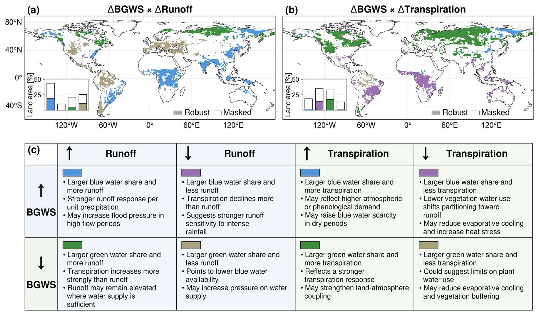
Figure 4 Projected changes in blue–green water partitioning and associated runoff and transpiration responses. Panels (a) and (b) show the ensemble mean ΔBGWS combined with changes in runoff and transpiration, respectively, for the end of the century relative to the historical period. Colours indicate the four joint sign combinations between ΔBGWS and the corresponding flux change, as defined schematically in panel (c), which also summarises their possible hydroecological implications. White grid cells in panels (a) and (b) denote areas excluded by the fixed historical analysis mask (Sect. 2.3) or masked because fewer than 8 of the 12 models agree on the same joint quadrant class. Insets show the land-area fraction of each quadrant class, with coloured bar segments indicating robust area and white segments indicating area masked because of low agreement.

3.4 Implications of future BGWS trends

The BGWS metric is a process rather than a quantity indicator. It characterises how an incremental unit of precipitation (e.g., the next millimetre of rain) is partitioned between runoff (blue water) and plant use via transpiration (green water), not how large those fluxes are in absolute terms. In this sense, BGWS addresses the question “where does the next unit of rain tend to go?” rather than “how much water is there overall?”. As our analysis excludes hyper-arid and sparsely vegetated regions, this distinction matters for impacts that depend on hydrological sensitivity and timing (Nijssen et al., 2001). It shifts the focus from one on absolute change, to one in which we try to understand controlling factors and enables another level of model evaluation that centres on comparing these controlling factors rather than just focusing on matching historical observations (Wagener et al., 2022). Although our analysis is flow-based and excludes storage terms, persistent BGWS shifts signal sustained pressure on blue water stores (e.g., rivers, reservoirs, groundwater) versus green water stores (root-zone moisture).

BGWS changes become most meaningful when interpreted jointly with absolute changes in runoff and transpiration rather than in isolation (Fig. 4). In combination with runoff changes (Fig. 4a), the robust sign combinations point to four distinct hydrological implications. Where ΔBGWS and ΔR are both positive, both runoff volume and the runoff share of precipitation increase, indicating stronger blue-water partitioning and greater potential for high-flow pressure during wet periods (e.g., southern Asia); where ΔBGWS is positive but ΔR is negative, runoff shrinks in absolute terms but its share of precipitation still increases. Thus, the relative contribution of runoff pathways per unit precipitation increases, indicating higher runoff sensitivity to intense rainfall. Yet, this pattern occurs only rarely in the robust map. Conversely, negative ΔBGWS with positive ΔR suggests more total runoff but a smaller share of precipitation, implying that runoff may remain elevated if water supply stays sufficient (e.g., northwestern Eurasia); where both ΔBGWS and ΔR are negative, shrinking blue water volumes and shares indicate concurrent pressure on blue-water supply (e.g., large parts of Europe). Comparable patterns are seen during European droughts, where blue water declines outpace green water responses, tightening low-flows even when vegetation maintains transpiration (Orth and Destouni, 2018).

Joint interpretation of BGWS with transpiration changes adds eco-physiological and land-surface insight (Fig. 4b). Where ΔBGWS and ΔE_t are both positive, landscapes become more runoff-dominated while plant water use rises, consistent with higher atmospheric/phenological demand and greater reliance on stored water (e.g., northeastern Eurasia); where ΔBGWS is positive and ΔE_t is negative, partitioning shifts toward runoff as vegetation down-regulates (e.g., southeastern South America). The latter response reduces evaporative cooling and elevates heat risk (He et al., 2022). Conversely, where ΔBGWS is negative and ΔE_t is positive, regions experience greener partitioning, which may strengthen land–atmosphere coupling and support stronger latent cooling (e.g., northeastern North America); when both ΔBGWS and ΔE_t decrease, relative allocation to green water rises despite lower plant water use, which points to weaker evaporative cooling and vegetation-mediated buffering of heat and moisture stress (e.g., parts of the Amazon rainforest).

In communicating results, it is important to make uncertainty explicit. Figure 4 therefore only shows areas where at least eight of the twelve models agree on the sign of both ΔBGWS and the corresponding flux change. Even so, the results should be read as robust regional tendencies rather than local predictions. In regions with robust sign agreement, joint interpretation of ΔBGWS with ΔR and ΔE_t provides a compact way to distinguish whether future change is more likely to intensify runoff sensitivity, strengthen transpiration demand, or simultaneously reduce water availability and vegetation cooling. Given the additional baseline biases relative to reanalysis and observation-based products (Sect. S3), a regionalised and observationally constrained analysis of ΔBGWS and co-varying hydroecological responses would still be needed before drawing site-specific management conclusions.

4 Conclusions

In this study, we assessed where future blue–green water partitioning shifts favour blue or green water pathways and which climatic and hydroecological changes are associated with these shifts. To do so, we defined the BGWS and applied it to 12 CMIP6 ESMs under SSP3–7.0, focusing on vegetated and hydrologically active land areas. Together, the results show distinct historical partitioning regimes, spatially heterogeneous future shifts, and a dominant role of precipitation intensification that is partly counteracted by vegetation expansion.

Historically, BGWS separates cold, high-altitude, and strongly seasonal regions with larger blue water shares from many water-limited regions with larger green water shares. Future changes show a slight ensemble-mean shift towards larger blue water shares, with strengthening or weakening of existing regimes more common than full regime shifts. The main predictor of projected BGWS change is increasing extreme five-day precipitation, which favours larger blue water shares, while increasing LAI provides the main counterweight by favouring vegetation-mediated green water use. Interpreting BGWS together with absolute runoff and transpiration changes helps distinguish where future changes may increase runoff sensitivity, strengthen vegetation water use, reduce blue water availability, or weaken vegetation-mediated cooling.

Nonetheless, uncertainties and biases in ESM studies remain because BGWS dynamics depend on the representation of hydroclimatic and biogeochemical processes (Clark et al., 2015; Gentine et al., 2019; Zheng et al., 2019; Padrón et al., 2022; Yang et al., 2023; Gier et al., 2024). An additional source of uncertainty is that many large-scale land models used in ESMs still represent lateral groundwater redistribution only in a limited or highly simplified way, partly because coarse model resolution does not resolve subgrid land-surface heterogeneity well (Liao et al., 2025). This can affect blue–green water partitioning by underrepresenting shallow groundwater support to ET during dry periods, potentially favouring a more blue-biased partitioning (Maxwell and Condon, 2016).

Despite these uncertainties, particularly in the land-surface components and their assumptions regarding plant responses to elevated CO₂, robust signals of BGWS shifts within the ESM ensemble emerge. While we used LAI as a proxy for vegetation responses that reflect both climatic and human influences, future research could assess land-use and land-cover changes more explicitly. Additionally, advancing both observational data and ESMs appears vital to improve the reliability of future projections on terrestrial freshwater availability, including a more consistent treatment of human influences such as irrigation. Coupling these advances with process-based ESM evaluations can deepen insights into blue–green water partitioning and vegetation–climate feedbacks and support more robust climate information, especially in understudied, high-impact regions (Stein et al., 2024).