Chaotic fluctuations in Greenland ice streams limit predictability of ice sheet collapse

The future evolution of the Greenland ice sheet (GrIS) depends on the rate and intensity of climate change and can transition to a mostly ice-free state under strong enough global warming. By applying different rates of temperature change in a state-of-the-art ice-sheet model coupled to a regional energy-moisture balance atmospheric model, oscillations in the total ice-sheet volume are found under warming magnitudes between 1.0 and 1.3 K above present-day temperatures. These oscillations are due to two ice streams located in the northern GrIS that each alternate between fast streaming and stagnation, manifesting in build-up/surge variability. These ice streams interact due to their spatial proximity, resulting in irregular periodicity. The ice streams are situated in a region where the collapse of the GrIS to an ice-free state initiates, impacting the time it takes before this transition occurs. For a fixed warming magnitude and an ensemble of warming rates and initial conditions, the timing of the collapse can differ by tens or hundreds of thousands of years. This delay is proposed to be due to a chaotic transient, suggesting that ice-stream oscillations are a potential source of internal chaotic variability in ice sheets and can complicate prospects of anticipating a collapse.

1 Introduction

The Greenland ice sheet (GrIS) is one of the principal tipping elements in the Earth's climate system (Armstrong McKay et al., 2022), meaning it could experience a massive and potentially irreversible change when an external forcing parameter, specifically the global mean temperature, increases beyond a critical threshold known as a “tipping point” (Robinson et al., 2012). Tipping of the GrIS involves the large-scale loss of ice mass (or “collapse” of the ice sheet) through melting and has a straightforward impact on the rest of the Earth by raising the global sea level (Gregory et al., 2004; Rignot et al., 2011; Wunderling et al., 2021).

Tipping of the GrIS can occur due to the presence of two strong positive feedbacks: First, a decrease in ice-sheet thickness leads to the temperature of the ice surface increasing, promoting further melting. This is known as the melt-elevation feedback. The second is the decrease of the surface albedo as a result of the melt of the ice sheet, and is known as the melt-albedo feedback. In a stable equilibrium state, where the ice sheet is in mass balance, the processes must be dominated by negative feedbacks: As atmospheric temperatures increase, so do precipitation rates, leading to a thickening of the ice sheet. Furthermore, the melt-elevation feedback is reduced by the effect of glacial isostatic adjustment: when ice thins, the resulting bedrock uplift partially compensates the reduced surface elevation. Uplift rates on the order of millimeters per year (Wake et al., 2016) mean that this effect is relevant on time scales of millennia or longer (Zeitz et al., 2022).

The feedbacks that determine the stability of the GrIS are influenced strongly by the surface air temperature of Greenland, which is increasing at a rapid pace (Intergovernmental Panel On Climate Change (IPCC), 2023). As it increases, the negative feedbacks that maintain the ice-covered state weaken, and at the tipping (or bifurcation) point the positive feedbacks accelerate mass loss and cause a transition to an ice-free state. This phenomenon is termed “bifurcation-induced tipping” (b-tipping). Although the bifurcation point of the GrIS has been assessed in different studies (Gutiérrez-González et al., 2026; Höning et al., 2023; Robinson et al., 2012; Zeitz et al., 2022), the effect of the rate of change of the forcing on tipping behavior has only been investigated for the Antarctic ice sheet (Feldmann et al., 2025; Swierczek-Jereczek et al., 2025). In non-autonomous systems with multiple dynamic time scales, increasing forcing at rates that are large compared to the time scale of negative feedbacks could lead to a tipping of the system at a forcing value less than the bifurcation point, a phenomenon known as “rate-induced tipping” (r-tipping) (Ashwin et al., 2012; Feudel, 2023).

The bulk of the GrIS evolves over time according to slow shear flow, but areas of fast flowing ice, such as topographically confined outlet glaciers or large ice streams, represent a source of variability with a faster dynamic timescale. Ice streams, which are characterized by sliding of ice at the base due to lubrication over a hard base or deformation of a till that is saturated with water, are particularly relevant. A fast warming rate can lead to an easier saturation of the base with water that cannot be compensated by drainage from under the ice sheet, thus activating ice streams and increasing mass loss. The discharge of ice through ice streams contributes substantially to the total ice-sheet mass loss despite their relatively small spatial extent (The IMBIE Team, 2020; Van Den Broeke et al., 2009). Furthermore, ice streams have accelerated due to increased atmospheric and oceanic forcings, contributing up to 50 % of the GrIS mass loss in the last decades (Box et al., 2022; Howat et al., 2008; Khan et al., 2014, 2022; Larocca et al., 2023; Luthcke et al., 2006; Rignot and Kanagaratnam, 2006; Rignot et al., 2011; Trusel et al., 2018).

Rate-induced tipping of Earth system components has previously been investigated in comprehensive models of the Atlantic Meridional Overturning Circulation (AMOC) (Lohmann and Ditlevsen, 2021) and the west Antarctic ice sheet (Feldmann et al., 2025; Swierczek-Jereczek et al., 2025). The rate of forcing is also important when considering the possibility of preventing a transition after overshooting a tipping point by imposing a subsequent cooling (Bochow et al., 2023). In this study, we use a state-of-the-art ice-sheet model coupled to a regional atmospheric energy-moisture balance model to investigate the GrIS response under different magnitudes and rates of warming in order to determine whether r-tipping of the GrIS is possible.

2 Methods

2.1 Model description

The model used in this study is the three-dimensional thermomechanical ice-sheet model Yelmo (Robinson et al., 2020, 2022) coupled with the regional energy-moisture balance climate model REMBO (Robinson et al., 2010) at the ice-sheet surface. This model setup is similar to that of Robinson et al. (2012) but with a different ice-sheet model, and has also been used in the study of Gutiérrez-González et al. (2026). The model domain covers the entirety of Greenland at a horizontal resolution of 16 km.

A full description of the ice-sheet model is not repeated here. Instead we focus this section on an illustration of the processes present at the base of the ice that are most important for the results of this article and which rely on several parameterizations. The Stokes stress balance equations that solve for the dynamic evolution of the ice sheet are parametrized as a combination of shear flow when the base of the ice is frozen to the bedrock (such that basal velocity is zero) and regions where there is sliding at the base (either for floating ice or ice streams) (Robinson et al., 2022). Thus, ice streams can be identified in model simulations by regions of grounded ice with nonzero basal velocity.

The basal frictional stress τ_b that resists basal sliding is modeled using a regularized Coulomb friction law (Schoof, 2005; Joughin et al., 2019),

$$\begin{array}{}\text{(1)}& {\mathit{\tau }}_{\mathrm{b}}=-c_{\mathrm{b}}({\displaystyle \frac{\left|{\mathit{u}}_{\mathrm{b}}\right|}{\left|{\mathit{u}}_{\mathrm{b}}\right|+u_{\mathrm{0}}}}{)}^q{\displaystyle \frac{{\mathit{u}}_{\mathrm{b}}}{\left|{\mathit{u}}_{\mathrm{b}}\right|}},\end{array}$$

where u_b is the two-dimensional basal velocity vector. The threshold speed u₀ = 100 m a⁻¹ allows the basal stress to saturate at high velocities, where it becomes independent of the basal velocity (Zoet and Iverson, 2020). Its value, along with the empirical parameter q=0.2, is derived from laboratory experiments (Zoet and Iverson, 2020). The bed friction coefficient c_b is a field that depends linearly on the effective pressure N at the base of the ice,

$$\begin{array}{}\text{(2)}& c_{\mathrm{b}}=\mathit{\lambda }N.\end{array}$$

The factor λ represents the till strength of the bedrock and depends on the elevation above or below sea level. This factor leads to larger sliding velocities at lower elevations, as the till in these areas is primarily composed of sediments that are softer and more easily deformable. A similar elevation-dependent till strength is also seen in Albrecht et al. (2020), Blasco et al. (2024), and Martin et al. (2011).

The effective pressure $\widehat{N}$ differs from the overburden pressure P₀ depending on the basal water saturation fraction $s\in [\mathrm{0},\mathrm{1}]$,

$$\begin{array}{}\text{(3)}& \widehat{N}=N_{\mathrm{0}}({\displaystyle \frac{\mathit{\delta }{P}_{\mathrm{0}}}{N_{\mathrm{0}}}}{)}^s{\mathrm{10}}^{\frac{e_{\mathrm{0}}}{C_{\mathrm{c}}}(\mathrm{1}-s)},\end{array}$$

following the parameterization of Bueler and van Pelt (2015). The parameter δ=0.02 is an empirical scaling factor of the overburden pressure. This means that the effective pressure at the base is equal to 2 % of the overburden pressure when the till is saturated (s=1), and any excess water is considered to be drained from the system (Bueler and van Pelt, 2015). The parameter N₀ = 1000 Pa is a reference pressure at reference void ratio e₀=0.69, and C_c=0.12 is the coefficient of compressibility of the till. Finally, since the overburden pressure is an upper limit for the effective pressure, the minimum of the two is taken,

$$\begin{array}{}\text{(4)}& N=min\mathit{\{}{P}_{\mathrm{0}},\widehat{N}\mathit{\}}.\end{array}$$

The basal water layer thickness H_w has a maximum value of H_w,max = 2 m, and the saturation fraction is defined as $s=H_{\mathrm{w}}/H_{\mathrm{w},\text{max}}$. In turn, H_w changes with the basal mass balance ${\dot{b}}_{\mathrm{g}}$ and is removed via a constant drainage rate C_d,

$$\begin{array}{}\text{(5)}& {\displaystyle \frac{\partial H_{\mathrm{w}}}{\partial t}}=-{\displaystyle \frac{{\mathit{\rho }}_{\mathrm{i}}}{{\mathit{\rho }}_{\mathrm{w}}}}{\dot{b}}_{\mathrm{g}}-C_{\mathrm{d}},\end{array}$$

where ρ_i and ρ_w are the densities of ice and water, respectively, and

$$\begin{array}{}\text{(6)}& {\dot{b}}_{\mathrm{g}}=-{\displaystyle \frac{\mathrm{1}}{{\mathit{\rho }}_{\mathrm{i}}L}}(Q_{\mathrm{b}}+k{\displaystyle \frac{\partial T}{\partial z}}{|}_b+Q_{\text{r}}).\end{array}$$

The function ${\dot{b}}_{\mathrm{g}}$ therefore converts the heat flux at the base to a melt rate via the latent heat of ice fusion, L. This heat flux consists of the heat generated by friction due to sliding of the ice along the base, Q_b, as well as the heat conducted into the column of ice above given by the coefficient of conduction of ice k and the temperature gradient of the ice at the base, $\frac{\partial T}{\partial z}{|}_{\mathrm{b}}$. In addition to this, there is a geothermal heat flux boundary condition Q_geo imposed 2 km below the surface, and the heat diffuses vertically through the bedrock. The term Q_r is then the flow of heat into the ice at the interface of bedrock and ice. The isostatic adjustment of the bedrock under the ice sheet uses the elastic lithosphere-relaxing asthenosphere (ELRA) model (Le Meur and Huybrechts, 1996) with a relaxation timescale of 3000 years.

At the ice-sheet surface, Yelmo is coupled to REMBO (Robinson et al., 2010). REMBO is a two-dimensional model with vertically integrated equations for energy and moisture balance. These variables are diffused throughout the model domain to represent processes at the dominant synoptic scale. The strength of this diffusion decreases with increasing latitude to represent decreased atmospheric activity at higher latitudes. REMBO also accounts for orography, whereby precipitation rates increase as the horizontal surface gradient increases. The temperature and precipitation fields of REMBO are calculated at 100 km resolution, and a bilinear interpolation is used to input these as boundary fields to the surface of Yelmo.

Ice sheets lose mass through dynamic processes such as ice streaming and calving of floating ice, but also through a negative surface mass balance (SMB). The SMB is the difference between the mass gained by precipitation in the form of snowfall and lost due to ablation, either due to melting, sublimation, or wind erosion. In the model, the SMB is determined by the air temperature at the ice-sheet surface and precipitation rates calculated by REMBO. The SMB can be separated into a positive contribution from precipitation and a negative contribution from surface melt M_s. The latter is calculated using an insolation-temperature melt method (ITM), in which insolation S and albedo α_s are explicitly taken into account (Bintanja et al., 2002):

$$\begin{array}{}\text{(7)}& M_{\mathrm{s}}={\displaystyle \frac{\mathrm{\Delta }t}{{\mathit{\rho }}_{\mathrm{w}}{L}_{\mathrm{m}}}}\left[{\mathit{\tau }}_{\mathrm{a}}\right(\mathrm{1}-{\mathit{\alpha }}_{\mathrm{s}})S+c+\mathit{\lambda }T],\end{array}$$

where Δt is the length of a day in seconds, ρ_w is the density of water, and L_m is the latent heat of melting. The atmospheric transmissivity ${\mathit{\tau }}_{\mathrm{a}}=\mathrm{0.46}+\mathrm{0.00006}{z}_{\mathrm{s}}$ is a function of the surface elevation z_s, increasing absorption of solar radiation with altitude and thereby acting as a negative feedback for large ice-sheet thicknesses. The surface albedo is calculated as

$$\begin{array}{}\text{(8)}& {\mathit{\alpha }}_{\mathrm{s}}=min({\mathit{\alpha }}_{\mathrm{g}}+{\displaystyle \frac{d}{d_{\text{crit}}}}({\mathit{\alpha }}_{\mathrm{s},max}-{\mathit{\alpha }}_{\mathrm{g}}),{\mathit{\alpha }}_{\mathrm{s},max}),\end{array}$$

where ${\mathit{\alpha }}_{\mathrm{s},max}$ is the maximum albedo of snow and α_g is the albedo of the ground, and $\frac{d}{d_{\text{crit}}}$ is the ratio of snow thickness d to a maximum value d_crit. Finally, c and λ are free parameters that fit surface temperature T to present-day melt rates of the GrIS (Robinson et al., 2010).

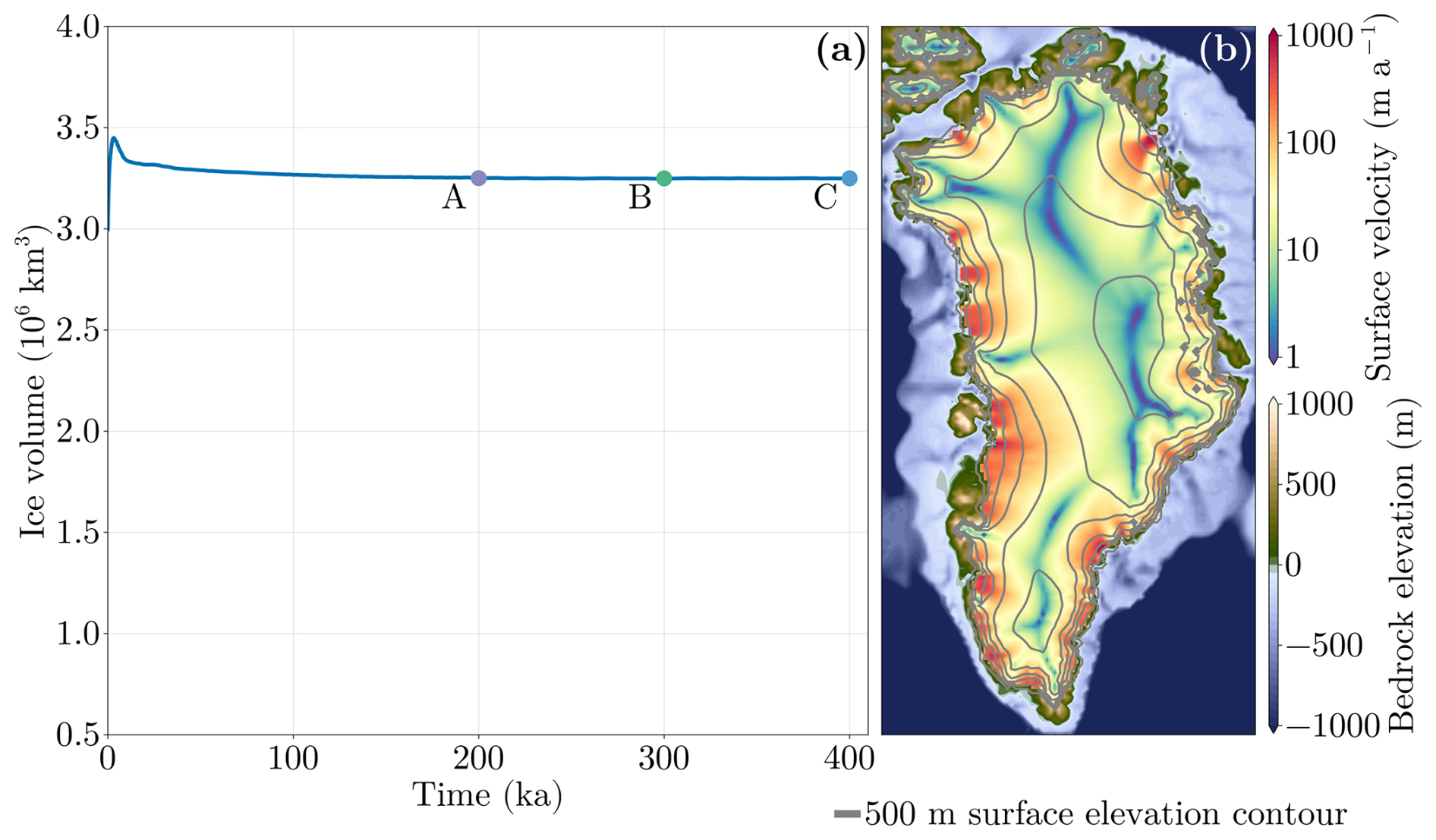
Figure 1 (a) Ice volume time series of the spinup simulation. The ice-sheet volume of three initial states A to C are shown. (b) Ice-sheet extent and surface velocities of the initial state  A.

2.2 Experimental setup and boundary conditions

To investigate r-tipping of the GrIS, an equilibrated initial state is required. This allows us to disentangle r-tipping from any effects of inertia associated with transient systems approaching equilibrium. The present-day GrIS simulation is initialized using ice-sheet thickness and bedrock topography from version 5 of the BedMachine mapping of Greenland (Morlighem et al., 2017) and the ERA-40 climatology (Uppala et al., 2005) as boundary conditions for REMBO, and allowed to relax to an equilibrium state over a 200 ka simulation. This equilibrated initial state is shown in Fig. 1. A comparison of the surface velocities of this initial state to those of the present-day GrIS (Joughin et al., 2018) is seen in Appendix Fig. 13. The states of the GrIS at 300 and 400 ka are also saved as initial states B and C, respectively, representing a small perturbation to initial state A. A comparison of the surface elevations and surface velocities of the three initial states is found in Fig. 14. The use of an ensemble of multiple initial states is not common for ice-sheet simulations, but is implemented to test the robustness of the results and a possible dependence on initial conditions.

The model is externally forced in subsequent experiments by applying a constant summer temperature anomaly to the surface temperature and an annual mean ocean temperature at the boundary of the model domain of REMBO, as in Gutiérrez-González et al. (2026) and Robinson et al. (2012). This regional summer surface temperature anomaly is approximately equivalent to a global mean temperature increase. Since r-tipping occurs for a forcing temperature less than the bifurcation point value, the latter must first be estimated. To this end, an adaptive quasi-equilibrium forcing (AQEF) function is used. The AQEF is a transient simulation with a variable forcing rate, and is implemented as such: The GrIS is considered to be quasi-equilibrated when the rate of mass loss of the last 100 years of model time is less than 2 Gt a⁻¹. While the ice sheet is not in quasi-equilibrium, the forcing is kept constant to allow it to reach quasi-equilibrium. Once quasi-equilibrated, the forcing is increased in an adaptive manner: the longer it takes the model to achieve quasi-equilibrium, the less the forcing is increased. The maximum rate at which the forcing can be increased is 10⁻⁵ K a⁻¹, and the minimum rate is 0. In this way, the forcing parameter does not increase while the collapse of the ice sheet is occurring, preventing rate-dependent hysteresis (An et al., 2021).

Once the bifurcation point has been estimated, it is used to determine a range of parameters for the subsequent ramping experiments that are used to assess the possibility of r-tipping. In these ramping experiments, the forcing is increased at a linear rate to some value less than the bifurcation point. Thereafter, the forcing is kept constant and the ice sheet is allowed to equilibrate over 400 ka. An ensemble of simulations is generated by applying different rates of increase and maximal forcing values, allowing the effect of the rate and magnitude of warming to be evaluated. These ramping experiments are also performed starting at each of the three initial states to investigate the dependence on initial condition.

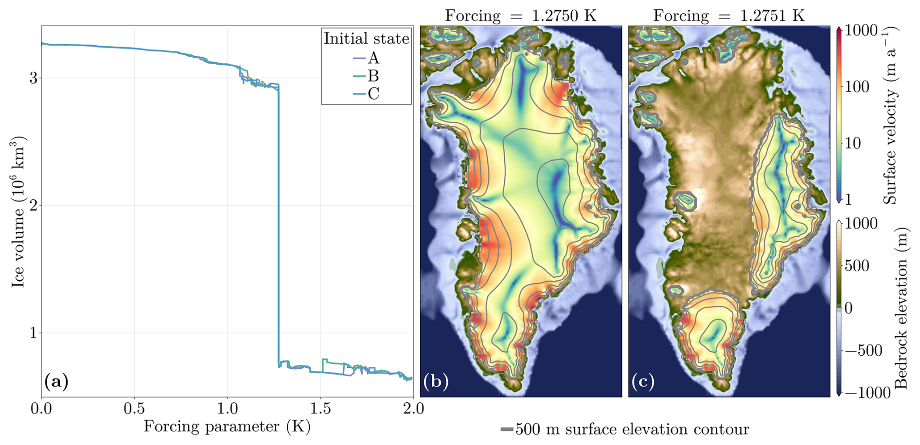
Figure 2 (a) Quasi-equilibrium ice volume of the GrIS as a function of the applied regional summer temperature anomaly in parameter space to estimate the b-tipping value for initial states A to C. (b) Ice-sheet before tipping. (c) Ice-sheet after tipping.

3 Results

3.1 Tipping of the ice sheet

Figure 2 shows the ice volume as a function of the forcing parameter, the regional summer temperature anomaly, for the three initial states. There is a clear tipping behavior for a forcing of +1.28 K, and it is essentially independent of the choice of initial state. This tipping resembles what is expected for a saddle-node bifurcation.

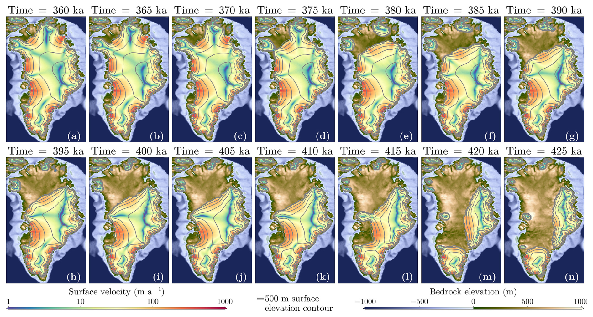
Figure 3 Ice-sheet extent and surface velocities during the tipping event at a fixed forcing value of +1.28 K.

The retreat of the GrIS during the tipping event is seen in Fig. 3. Spatially, the retreat begins in the north. The spatial tipping pattern is equivalent to that of Robinson et al. (2012). The pattern of ice-sheet loss is also similar to that of Zeitz et al. (2022) (their Fig. 3b) albeit without eventual partial regrowth of the ice sheet after collapse (their Fig. 3c).

Figure 4 Time series of the forcing amplitude during the ramping experiments.

3.2 Ramping experiments

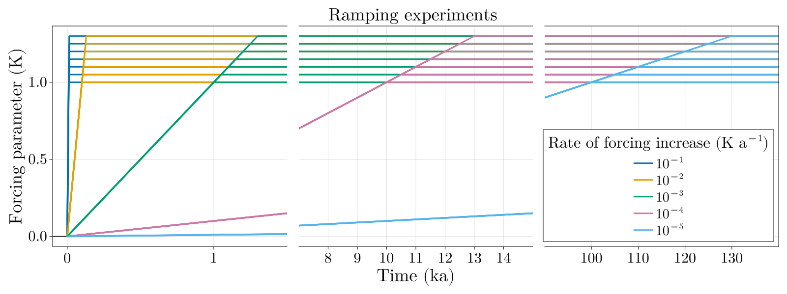
The estimated bifurcation point is used to inform the parameter range for the ramping experiments. Since the bifurcation point is located at +1.28 K, the maximal forcing of the ramping experiments are chosen as +1.00, 1.05, 1.10, 1.15, 1.20, and 1.25 K. A value of +1.30 K past the bifurcation point is also included to confirm that tipping does indeed always occur when forced past +1.28 K. The forcing increases linearly at a rate of 10⁻¹, 10⁻², 10⁻³, 10⁻⁴, or 10⁻⁵ K a⁻¹, up to one of the seven maximal forcing values noted previously. The time series of the forcing for each experiment are shown in Fig. 4.

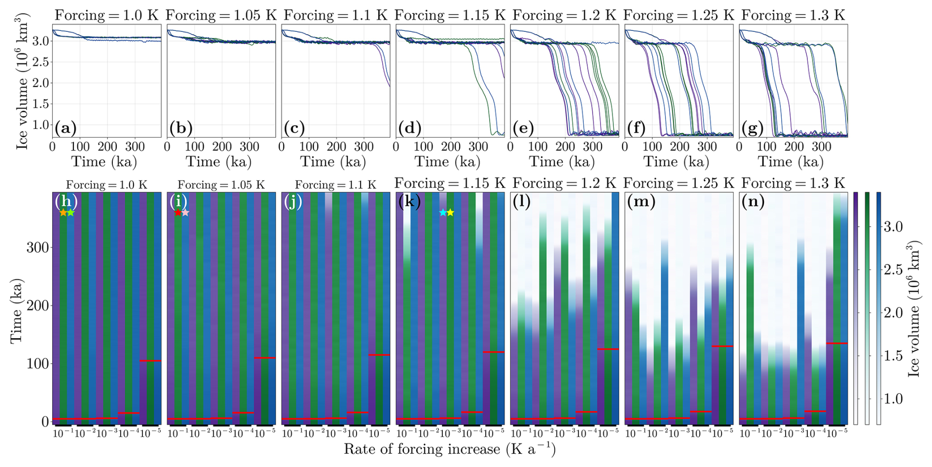
Figure 5 (a–g) Time series of the ice-sheet volume for all simulations to a given maximal forcing. (h–n) Time series of the ice sheet volume for all of the simulations grouped by maximum forcing value. The initial state of each simulation is indicated by the different colors: purple for A, green for B and blue for C. For a given maximal forcing, the simulations are ordered along the bottom axis in decreasing rate of forcing, with the red line indicating the time when the forcing reaches its maximum. The stars indicate simulations that appear in Figs. 7–11, B1–B3, and E1.

Each of the ramping experiments is initialized from one of three states A, B and C, and the entire ensemble consists of 7 × 5 × 3 = 105 members, which are all shown in Fig. 5. The appearance of tipping in Fig. 5c to f suggests rate-induced tipping, as tipping is observed for simulations forced to values lower than the b-tipping value of +1.28 K. Tipping also occurs for all simulations forced past the bifurcation point, that is, those forced to +1.30 K. What is absent, however, is some critical rate below which tipping does not occur, implying that r-tipping of the GrIS can occur even for very slow rates of forcing (Fig. 5l and n).

One prominent feature in this ensemble of simulations is the non-monotonicity in the time before the tipping occurs, hereafter referred to as the “tipping time”, with rate of forcing, magnitude of forcing, and initial condition. For the same initial conditions, longer tipping times are often seen for faster forcing rates. For instance, for initial condition C at a forcing level of +1.25 K, the trajectory forced at a rate of 10⁻² K a⁻¹ tips around 300 ka, where the trajectory forced at slower rate of 10⁻³ K a⁻¹ tips earlier, around 100 ka.

In addition, tipping times for a maximum forcing of 1.30 K can be longer than those for 1.25 K. For example, for initial condition B and the slowest rate of 10⁻⁵ K a⁻¹, the tipping occurs around 250 ka for a forcing of +1.25 K and around 400 ka for +1.30 K. Finally, even for the same magnitude of forcing and rate of forcing, the tipping times are not consistent over initial conditions. For example, the simulations forced to +1.20 K at a rate of 10⁻³ K a⁻¹ tip at 300, 350 and 250 ka for initial conditions A, B and C, respectively. Overall the tipping behavior seems to be sensitively dependent on the initial state of the system and the rate of forcing.

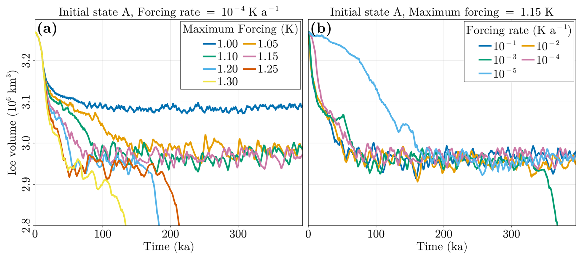
Figure 6 (a) Time series of ice volume for simulations with initial condition A, forcing rate 10⁻⁴ K a⁻¹, and a range of maximal forcing values. (b) Same as (a), but with a fixed maximum forcing of +1.15 K and range of forcing rates.

While investigating the cause of these random tipping times, irregular oscillations in the ice-sheet volume before tipping were observed. These oscillations can be isolated to a single region of the ice sheet: the northern drainage basin, where the ice-sheet also begins its retreat during a tipping event (Fig. 3a–d). It is hypothesized that the random tipping times are linked to these irregular oscillations. An example of the oscillations for each maximal forcing is shown in Fig. 6a. For all these simulations, there is an initial loss of mass during the first 50–80 ka of simulation time. Thereafter, for a maximal forcing of +1.00 K, there is a relatively small amount of variability around a steady ice volume of about 3.09 × 10⁶ km³. For maximal forcing values between +1.05 and +1.15 K, the mean ice volume is lower, between 2.9 and 3.0 × 10⁶ km³. The ice sheet experiences volume fluctuations with magnitudes on the order of 0.05 × 10⁶ km³ and periods between 8 and 30 ka. Finally, the simulations for maximal forcing of +1.20 to +1.30 K in Fig. 6 retreat to a much smaller ice volume, representing a collapsed GrIS as seen in Fig. 2c.

Figure 6b shows these oscillations for a fixed forcing magnitude of +1.15 K and varying rates of forcing, showing that the variability is not uniquely determined by the forcing magnitude, but is still similar in amplitude and period. Tipping for one of the rates (10⁻³ K a⁻¹) is also observed, albeit not for the fastest rate, as can be expected for r-tipping.

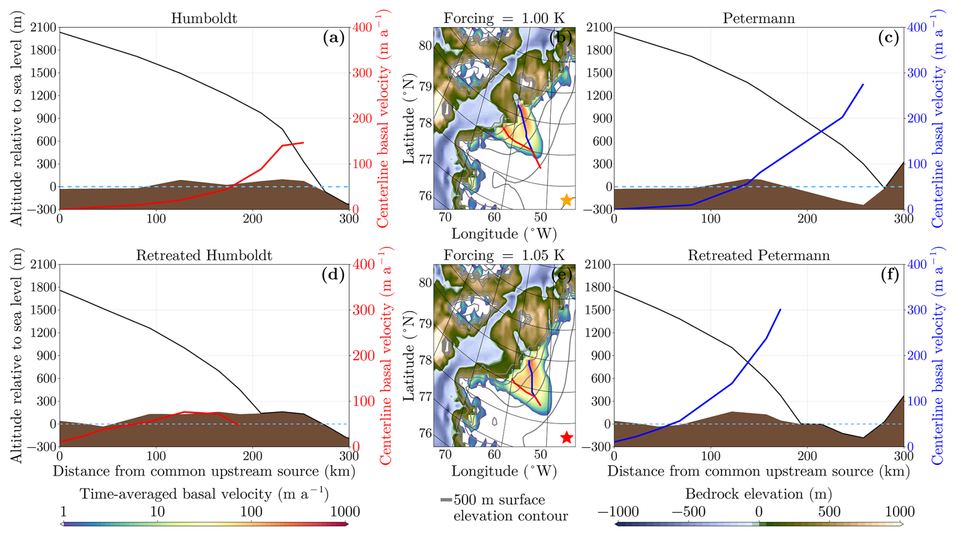
Figure 7 (a, c) Centerline ice-thickness profile (black) and basal velocities along the centerline for the HIS and PIS. (d, f) Same as (a, c) but for the retreated HIS and retreated PIS. (b, e) Time-averaged basal velocity field. The lines perpendicular to the gray height contours are the ice-stream centerlines for Humboldt (red) and Petermann (blue).

3.3 Spatial and temporal behavior of the oscillations

Two simulations at a forcing of +1.00 and 1.05 K are compared, as this represents the onset of the large-amplitude variability seen in panel (a) of Fig. 6. Further examination of the oscillations show they are a result of two ice streams that alternate between periods of stagnant and rapid basal sliding. These are the Humboldt and Petermann glaciers, which lie in close proximity to each other on the northern ice-sheet edge (Fig. 7). These glaciers are both regions of fast-flowing ice (Carr et al., 2015; Ehrenfeucht et al., 2023; Hillebrand et al., 2022) and behave as ice streams in the model simulations.

The first difference to be seen is the extent of the ice sheet in this region. For a forcing of +1.00 K, the ice-sheet margin is such that the Humboldt ice stream (HIS) is marine-terminating, with the Petermann ice stream (PIS) covering the Petermann fjord. The ice sheet in this case is termed “unretreated”. In the simulation with a forcing of +1.05 K, the ice sheet extent is much reduced. From the mean ice-thickness profiles, the ice margin is almost 100 km further inland (Fig. 7a, c, d and f). The HIS is no longer connected to the ocean, although the PIS terminates at the Petermann fjord. We refer to this as the “retreated” configuration, with the two separate ice streams designated as the retreated HIS and retreated PIS.

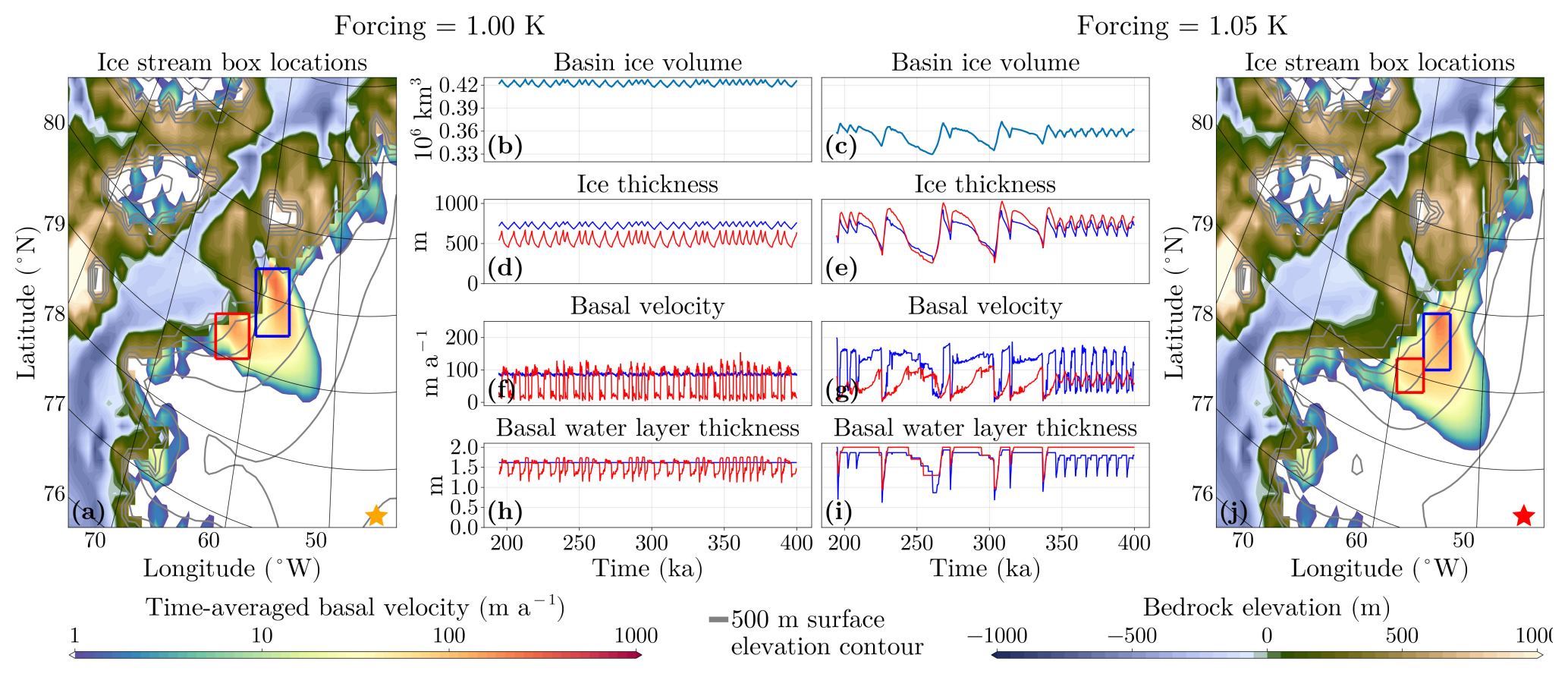
Figure 8 (a, j) Location of the PIS/retreated PIS (blue) and HIS/retreated HIS (red) ice-stream boxes superimposed over the temporal average of the basal velocity between 200 and 400 ka of the unretreated (a) and retreated (j) configurations. (b-i) Time series of basin ice volume, mean ice thickness, basal velocity, and basal water content in the ice-stream boxes in the unretreated (d, b, f, and h) and retreated (c, e, g, and i) configurations.

The temporal behavior of the unretreated and retreated configurations is compared by taking the spatial mean in two grid boxes, one containing the PIS/retreated PIS and the other the HIS/retreated HIS, as seen in Fig. 8a and j. For the unretreated case, the basal velocities in the two different ice streams behave quite differently. The PIS is in a state of steady flow of around 100 m a⁻¹, facilitated by a constant basal water layer thickness. The HIS, in contrast, alternates between near zero basal movement and sliding velocities of 100 m a⁻¹. The periods of stagnation correspond with an increase of basal friction caused by a reduction in the water content of the till due to freezing or drainage. While the basal velocities are minimal, the ice thickness increases, establishing a “build up” phase. The subsequent loss of mass due to rapid ice streaming is a “surge” phase. The period of these oscillations varies between approximately 5 and 9 ka. This steady cycle of mass gain during the build-up phase and loss during the surge results in an oscillation in mean ice thickness between 100 and 200 m in amplitude. The PIS also shows a smaller alternation in ice thickness with a similar temporal pattern while maintaining constant ice-stream flow, suggesting the thickness variations are influenced by the oscillations of the nearby HIS.

In the retreated configuration, the oscillations of ice thickness and basal velocity have larger amplitude and longer period, as mentioned previously. While the exact location of the retreated PIS and retreated HIS differs slightly in all the simulations showing oscillations, their existence is robust among the ensemble. In contrast to the unretreated PIS, the retreated PIS is no longer in a steady-flow state and instead displays the same build-up/surge variability as the unretreated and retreated HIS.

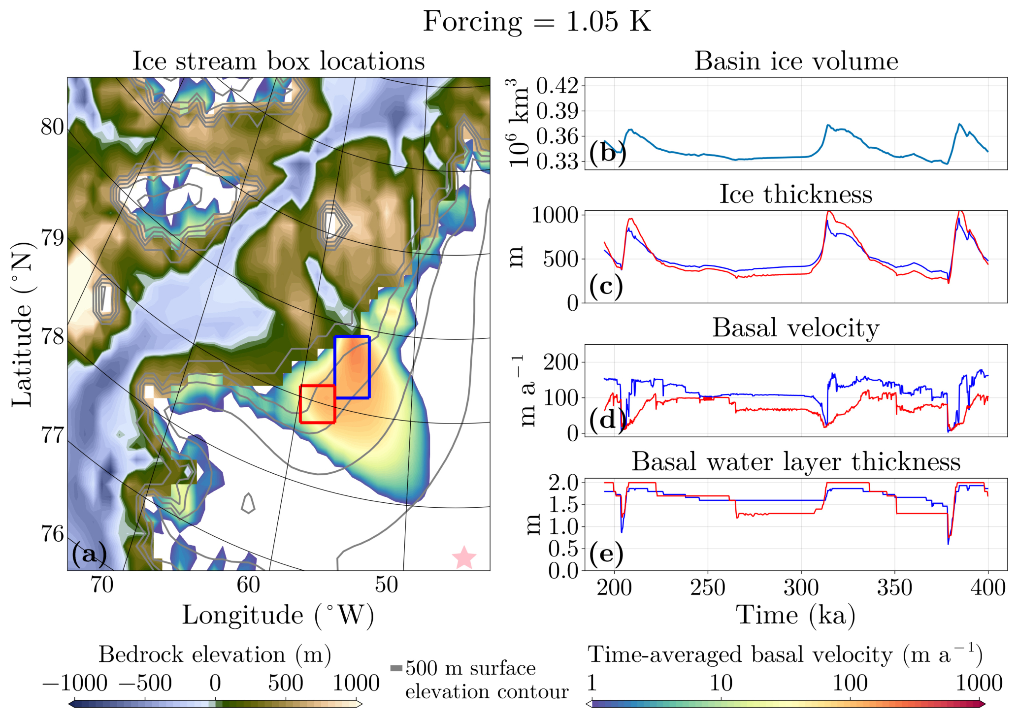
Figure 9 As Fig. 8, but starting at initial state C instead of B.

Two general patterns emerge for the oscillations of the retreated configuration. The first is one of a long, asymmetric build-up and surge event. An example is seen around 225 to 260 ka in Fig. 8c, e, g, and i. While the basal velocity in the retreated PIS switches abruptly between the build-up and surge phases, the basal velocity in the retreated HIS increases gradually. This accelerates mass loss until a point where the basal water layer thickness rapidly decreases in both ice streams when the ice thickness reaches its minimum, resulting directly from the thermomechanical coupling. The second pattern is that of short oscillations with a period of around 8 ka. These are seen in the last 60 ka of the time series in Fig. 8c, e, g, and i. The basal velocity in the retreated PIS abruptly switches between maximal and minimal, with corresponding drops in basal water-layer thickness when the velocity is minimal. In the retreated HIS, the till remains saturated with water. However, the basal velocity, and thus the flow, is not steady. It increases during the surge and decreases during the build-up of the nearby retreated PIS. This indicates an influence of the retreated PIS on the retreated HIS.

Thus the distinguishing factor between the two patterns is that during the short oscillations, the retreated PIS is in a build-up/surge mode, whereas the retreated HIS has a constant till saturation. This causes the retreated HIS to be in a steady-flow state, while still experiencing small oscillations due to the proximity to the retreated PIS. On the other hand, both the retreated HIS and the retreated PIS are in the build-up/surge mode during the longer-period events. A third mode is seen in some simulations that is shown in Fig. 9, and is identified by a long period of minimal ice volume. This mode corresponds to a steady flow state of intermediate mean basal velocities of around 100 m a⁻¹ in both the retreated HIS and the retreated PIS.

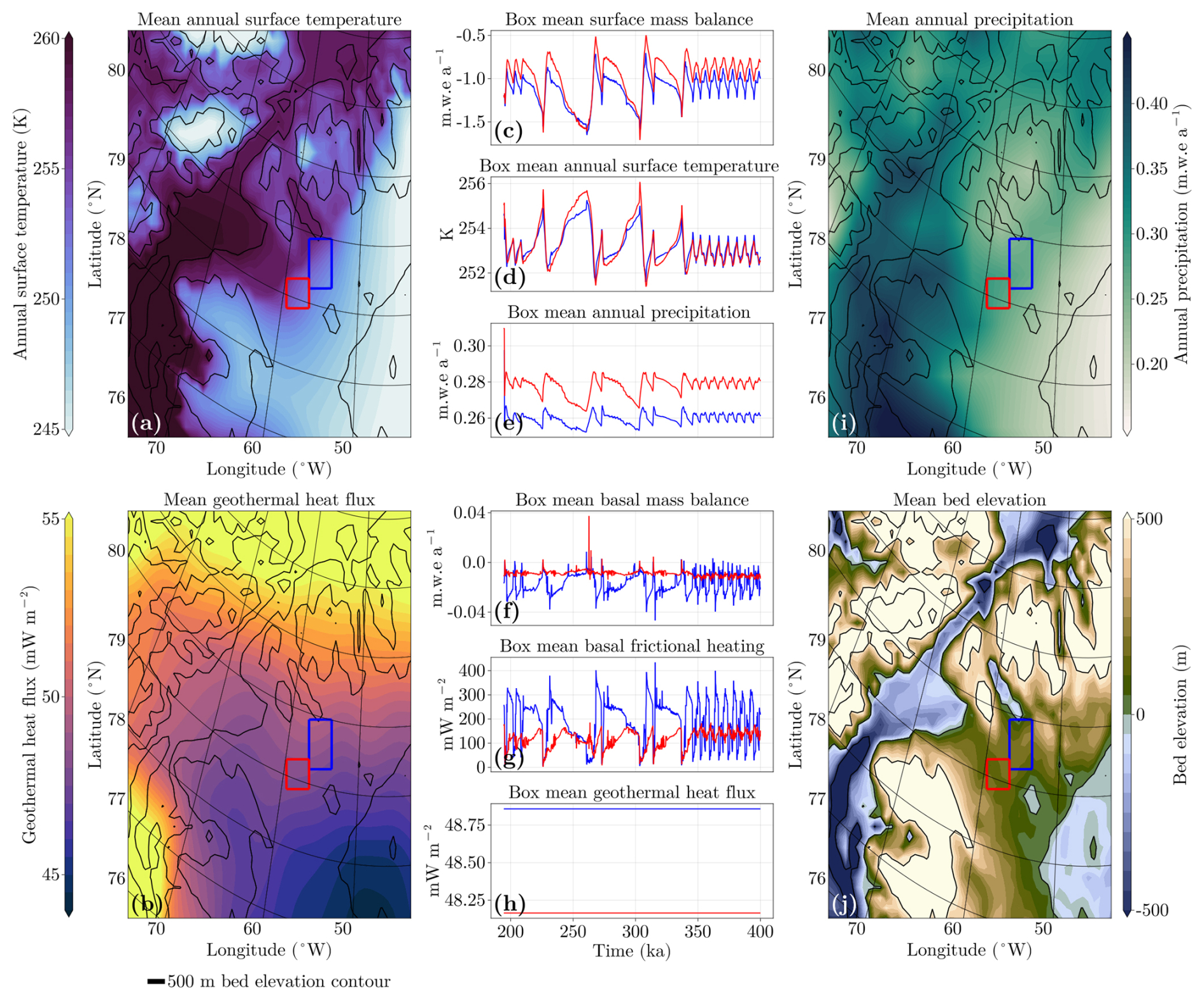
Figure 10 Location of the retreated PIS (blue) and retreated HIS (red) ice-stream boxes superimposed over the temporal average of annual surface temperature (a), geothermal heat flux (b), annual precipitation (e), and bed elevation (j). Time series of surface mass balance (c), annual surface temperature (d), annual precipitation (e), basal mass balance (f), basal frictional heating (g), and geothermal heat flux (h) in the ice-stream boxes.

The differences between the behavior of the PIS and the HIS in both configurations can be explained by slight variations in their topography and forcing fields, as seen in Fig. 10. The constant geothermal heat flux in the PIS is slightly higher than in the HIS, with a spatial average of 48.75 and 48.25 mW m⁻², respectively. During the periods where oscillations occur, the basal mass balance in the PIS varies much more than in the HIS, primarily due to the larger frictional heating (Q_b in Eq. 6) which is a direct result of larger basal velocities in the PIS while it is streaming (Fig. 10g). The bed elevation of the HIS is lower than the PIS, leading to lower average basal friction and thereby making it more prone to the steady-streaming state. Finally, the HIS receives more precipitation than the PIS on average, about 0.28 $\mathrm{m}.\mathrm{w}.\mathrm{e}.{\mathrm{a}}^{-\mathrm{1}}$ compared to 0.26 $\mathrm{m}.\mathrm{w}.\mathrm{e}.{\mathrm{a}}^{-\mathrm{1}}$, respectively. This might allow for the mass lost by the HIS during streaming to be better balanced by the accumulation, as opposed to the PIS, where lower accumulation means the ice thickness can only regrow once the streaming has quiesced.

Figure 11 Ice-sheet surface altitude, ice thickness, and bedrock altitude in the retreated HIS and PIS boxes of Fig. 8j.

3.4 Effect of glacial isostatic adjustment on the oscillations

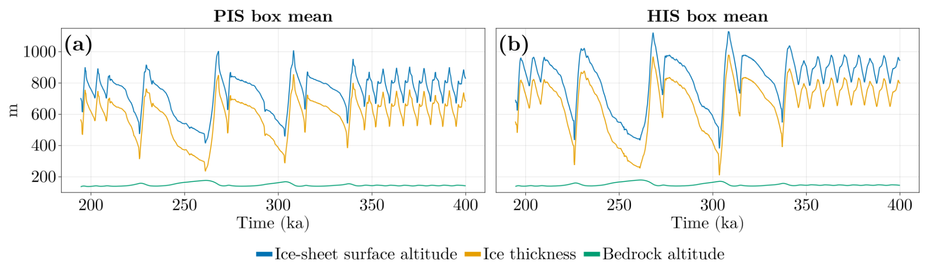
Glacial isostatic adjustment (GIA) has been demonstrated to cause oscillations in ice sheet volume (Petrini et al., 2025; Zeitz et al., 2022), and the relaxation time of 3000 years is relevant on the timescales of variability observed in the HIS and the PIS. Figure 11 shows the magnitude of variation in the altitudes of the bedrock and ice-sheet surface as well as the ice thickness. The maximum bedrock altitude in both the HIS and the PIS is close to 200 m, which is reached at the end of a long surge event (around 260 ka in Fig. 11). However, this value is only approximately 40 m greater than the minimum bedrock altitude at the beginning of the surge (around 230 ka in Fig. 11), meaning the bedrock is not the primary contributor to the difference in the surface altitude during the period of variability. In contrast, the ice thickness changes by about 600 m for the HIS and 500 m for the PIS during this time. So, while there is some effect of the GIA, the magnitude of the uplift of the bedrock is never so large as to affect the build-up/surge variability of the ice sheet. If the regrowth of the ice sheet after a surge were triggered by the GIA bringing the bedrock to an altitude that allows for a positive SMB, we may expect to see a period of minimal ice thickness during which the bedrock is uplifting, and at a certain altitude the ice thickness to start increasing again. Instead, we see the GIA simply lagging the ice thickness. The ice regrowth instead corresponds to a minimal basal velocity, i.e. an end of the surging. So, while the GIA does have some influence on the ice surface elevation, it does not set the pace of the oscillations.

3.5 Removal of the oscillations

To assess whether the lack of predictability of the tipping is due to ice-stream oscillations or due to other factors, we change the value of a parameter in the basal friction law to eliminate the tendency of ice streams to oscillate and investigate the consequences. As described previously, the ice-stream oscillations are surges in the basal velocity of the ice stream due to the thermomechanical coupling at the base of the ice sheet. To remove the oscillations but maintain the ice stream, the basal velocities in the region of interest need to be lower but non-zero. For lower basal velocities, the mass lost due to streaming is closer to the accumulation rate, bringing the ice stream to a steady flow state (Robel et al., 2013). To achieve this, the value of δ in Eq. (3) is increased. This raises the minimal effective pressure (Bueler and van Pelt, 2015) and thereby increases the basal frictional stress.

Increasing the value of δ and thereby the basal frictional stress has the effect of making the entire ice sheet less dynamically active, reducing the amount of mass loss due to ice streaming and calving. This means that the temperature forcing required to induce the collapse of the ice sheet is greater for larger values of δ.

Simulations with the original value of δ = 0.02 as well as increasing values of δ to 0.04 and 0.10 are shown in Fig. 12. As δ is increased, we note an increase in the oscillatory period until the oscillations disappear completely. As this factor affects ice streams across the entire ice sheet, the bifurcation point for each of these parameter values is different. Specifically, the bifurcation point increases as δ increases, as the ice sheet is losing less mass due to lower ice stream velocities.

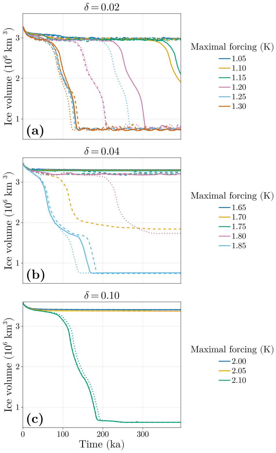
Figure 12 Time series of the ice sheet volume for increasing δ. For each value of δ, a range of forcing magnitudes at three rates starting from initial state A were applied: 10⁻¹ (dotted lines), 10⁻² (dashed lines) and 10⁻³ (solid lines) K a⁻¹.

For δ = 0.02, all (no) simulations with the strongest (weakest) forcing tip, but for intermediate maximum forcing values the tipping times do not decrease monotonically with the forcing rates. For a large enough value of δ = 0.1, the ice-stream oscillations disappear and the tipping time for a maximal forcing of +2.10 K occurs at approximately the same time for each rate. That is, the dependency on the forcing rates disappears and the tipping is much more predictable. This suggests that the ice-stream oscillations introduce a delay in the tipping.

4 Discussion

4.1 R-tipping of the GrIS

Accelerating mass loss is typically seen in marine-terminating outlet glaciers due to their sensitivity to oceanic forcing (Choi et al., 2021; Greene et al., 2024; Millan et al., 2023; Rignot et al., 2012; Wood et al., 2021), suggesting rate-induced effects may be more prevalent in these areas due to the fast timescale of the marine ice sheet instability (Feldmann et al., 2025; Schoof, 2007; Swierczek-Jereczek et al., 2025; Weertman, 1974). However, future loss due to negative SMB forced by increasing atmospheric temperatures could outweigh that of ice-sheet dynamics due to ocean forcing (Bevis et al., 2019; Enderlin et al., 2014). In addition, atmospheric forcing may be more critical in the north of Greenland compared to the south (Slater and Straneo, 2022), which is reflected in the model simulations. The ice extent shown in Fig. 3 indicates that mass loss does not start in regions with many marine-terminating outlet glaciers, specifically the southeast (Van Den Broeke et al., 2009). In fact, many remain after the tipping has completed. This indicates that the possibility of r-tipping of the GrIS primarily by oceanic forcing may not be relevant.

The remainder of the ice sheet interacts predominantly with the atmosphere, and the mass loss occurs either through surface melt or dynamically through ice streams which may not necessarily be marine-terminating, meaning the activation of ice streams does not depend on oceanic basal melting. The answer to whether the large-scale mass loss of the GrIS can be influenced by the sensitivity of these fast-moving ice streams to the rate of atmospheric warming is not entirely clear on the basis of the results of this study. There is no apparent critical forcing rate for which r-tipping occurs, at least not for a rate faster than 1 K of warming over 100 ka. The simulations indicate that the tipping behavior is affected by the rate of forcing but in a non-monotonic manner. However, the long tipping times are not explained by non-monotonic r-tipping (Ashwin et al., 2017), as we would expect any tipping events to occur at roughly the same time at a given forcing magnitude. While it may be valid to claim that r-tipping does indeed occur since the final state of the GrIS depends on the rate of forcing in some way, it is important to approach this point with nuance.

4.2 Ice-stream oscillations and chaos

Ice streams not only represent a mechanism of rapid mass loss in ice sheets, but have also been shown to be a source of internal periodic variability in models. Periodic behavior of ice masses can be seen in glaciers that are confined to some topographical valley and/or have a basal slope, for example Budd (1975); Kamb et al. (1985); Clarke (1987). Their reduced spatial extent also means their periodic behavior is on a much shorter time scale of decades to centuries and thus directly observable. While the same cannot be said of oscillating ice streams with periods of millennia, present-day ice streams have been demonstrated to be accelerating (Catania et al., 2012) or decelerating (Beem et al., 2014; Catania et al., 2006), due to thermomechanical coupling at the base of the ice sheet, see also Scambos et al. (2017). Studies of oscillatory behavior in ice sheets include parameterized models (Oerlemans, 1983; Fowler and Johnson, 1996; Payne, 1995; Robel et al., 2013) and comprehensive ice-sheet models with both idealized geometries (Calov et al., 2010; Feldmann and Levermann, 2017; Hank et al., 2023; Sayag and Tziperman, 2011; Souček and Martinec, 2011; Van Pelt and Oerlemans, 2012) and realistic topographies (Hank and Tarasov, 2024; Papa et al., 2006; Roberts et al., 2016; Schannwell et al., 2023). Additionally, some studies include a coupling to additional components of the climate system (Calov et al., 2002; Ziemen et al., 2019). Similarities between the oscillations seen in this paper and those observed in paleoclimate modeling studies are discussed in Appendix C.

Large-scale oscillations in the GrIS ice volume have been reported in the modeling studies of Zeitz et al. (2022) and Petrini et al. (2025), but the characteristics of those oscillations are an order of magnitude higher than what is seen in the present work, having periods over 100 ka and amplitudes between 0.4 and 2.1 × 10⁶ km³. The values of mantle viscosity and atmospheric lapse rate used in Yelmo and REMBO are 1 × 10²¹ Pa s and 6.5 K km⁻¹, respectively, which places it in the oscillatory regime of Zeitz et al. (2022) under moderate temperature forcing. As all three models use an ELRA model of glacial isostasy, the primary difference between the observed behavior in those studies compared to the present work is the regional atmospheric model. In Zeitz et al. (2022), the SMB is calculated using a positive degree day (PDD) method that depends on the surface temperature which is calculated locally as a function of the altitude. In Petrini et al. (2025), the SMB is calculated offline using the Community Earth System model, and then adjusted via a lapse rate during the runtime of the ice sheet model to reflect changes in ice sheet topography. However, there is no back-coupling of the ice sheet to the atmosphere. In contrast, REMBO allows for diffusion of energy and moisture, which decreases the local strength of the melt-elevation feedback, thereby also reducing the sensitivity to the GIA feedback.

Common to ice-sheet modeling is the use of a single initial state for a given combination of parameters rather than an ensemble. The use of an ensemble of states for investigating the evolution of an ice-sheet model is not too common, appearing in the studies of Tsai et al. (2017) and Verjans et al. (2025) to be able to account for the variability of the atmosphere and ocean when forcing the ice sheet. This is distinct to the results of this study, where the model is not coupled to an external climate model beyond a simple, deterministic diffusive energy and moisture balance atmosphere and thus the variability is internal to the ice sheet itself. That is, in those studies there is an external chaotic forcing that necessitates the use of an ensemble, whereas our model setup experiences constant external forcing after the temperature ramping period has ended. Despite the constant external forcing, we see simulations at a given forcing magnitude exhibit significant deviations from each other, indicating a sensitive dependence on the initial state which is a hallmark of an internal chaotic mode of variability.

While it is outside of the scope of the present study to formally prove that this mode of variability is indeed chaotic, there are some features that can be neatly interpreted as manifestations of chaos, particularly the unpredictable tipping times which are discussed in Sect. 4.3. Whether the chaos is a genuine physical phenomenon or simply a result of parameterization is under contention and will require further investigation. As this irregular variability of surging ice streams been reported in many other ice-sheet modeling studies, its existence is not entirely unfounded (Calov et al., 2002; Feldmann and Levermann, 2017; Hank et al., 2023; Hank and Tarasov, 2024; Papa et al., 2006; Roberts et al., 2016; Sayag and Tziperman, 2011; Souček and Martinec, 2011; Van Pelt and Oerlemans, 2012; Ziemen et al., 2019; Schannwell et al., 2023). What is unique to this study is the period and amplitude of the oscillations in the GrIS, as well as its switching between two different modes due to a coupling of nearby ice streams. The study of Kypke et al. (2026a) examines this variability using a simplified model, establishing that this chaos can arise in a system with no spatial extent.

An important caveat of the results of this paper is that oscillations in the model are highly sensitive to the basal friction parametrization. The physical mechanisms at the base of the ice that allow for ice streaming are not perfectly understood, and therefore the behavior of ice streams in models can depend heavily on the specific parameterization (Brondex et al., 2017, 2019). In situations where ice streams are marine-terminating, buttressing of ice shelves can serve to regulate the pace of mass loss, and thus decrease their sensitivity to the basal friction (Sun et al., 2020; van den Akker et al., 2026). Due to the lack of floating ice shelves that might provide buttressing in the HIS and PIS, it is to be understood that the oscillations are highly sensitive to the basal parameterization. Indeed, this is also reflected in the results of changing the parameter value of δ in Sect. 3.5, which is further discussed in Sect. 4.4. Further limitations are discussed in Sect. 4.5.

4.3 Chaotic transients

Due to the large mass of the ice sheet and the long timescales associated with surface mass balance processes, there is considerable inertia when transitioning from ice-covered to ice-free, especially when the system is kept very close to the tipping point. This causes the system to spend a long time in the ice-covered state after the bifurcation point has been passed, before eventually collapsing. If the ice sheet has an internal mode of chaotic variability, then the time spent before the collapse is sensitively dependent on the configuration of the ice sheet when the bifurcation point is crossed, and these transitions are called chaotic transients (Lai and Tél, 2011). The long and unpredictable tipping times seen in this study are proposed to be due to such chaotic transients, and they can obscure the detection of r-tipping.

The interplay between chaotic transients and r-tipping has been previously reported in a study by Lohmann and Ditlevsen (2021) for the AMOC. In their study, trajectories forced at different rates are brought close to the basin boundary between the stable “AMOC on” state and a chaotic saddle that separates it from the stable “AMOC off” state. This basin boundary is fractal, such that different rates of forcing may land the system differently on the saddle, where it experiences a chaotic transient resulting in transitions to the AMOC off state that are non-monotonic in rate. Alternatively, chaotic transients can arise due to a “ghost attractor” that appears for forcing values just past a bifurcation point, where the drift away from the ice-covered state, which is now no longer a stable fixed point, is slow (Strogatz, 1994). The oscillatory behavior of the build-up/surge variability can generate unstable periodic orbits that “collide” with the chaotic attractor of the ice-covered GrIS at the bifurcation point, generating the ghost attractor. Thus the chaotic transients in this study may either arise when crossing a chaotic saddle before the bifurcation point due to r-tipping, or due to being caught in a ghost attractor after passing a bifurcation point (i.e. b-tipping).

To answer the question of whether the GrIS experiences r-tipping in the ramping experiments, we must examine the chaotic transients. The system-specific critical forcing value was estimated as +1.28 K, and multiple simulations were observed to experience tipping for a forcing value less than this but with a fast rate of change of the forcing, implying r-tipping. However, the adaptive quasi-equilibrium forcing itself may exhibit a chaotic transient, which would result in overestimation of the bifurcation point. Comparing the simulations ramped to +1.25 K (below the assumed critical value) and +1.30 K (above the assumed critical value), we note that they are similar in oscillatory amplitude and period before tipping. If the oscillations are due to crossing a chaotic saddle before the assumed bifurcation point of +1.28 K, and therefore r-tipping, then they must be qualitatively different from the behavior of the system after the bifurcation point is passed. Since the variability of the simulations at the two forcing values are qualitatively similar in period and amplitude, we conclude that they are generated by similar non-attracting sets (Lai and Tél, 2011). This implies that the critical value is not between +1.25 and 1.30 K as estimated by the AQEF. This reasoning can be extended to all parameter values that result in tipping (i.e. +1.10 to +1.30 K). Thus, either the bifurcation point is between +1.05 and 1.10 K and all transients are due to a ghost attractor, or the bifurcation point is larger than +1.30 K and all of the transients are due to an r-tipping through a chaotic saddle.

The behavior of the chaotic transients in the present study more closely resembles those due to a ghost attractor after a bifurcation than due to r-tipping through a chaotic saddle. First, scaling laws indicate that the lifetime of the chaotic saddle, and thereby the tipping time, should increase as the maximal forcing approaches the bifurcation point (Mehling et al., 2024). In contrast, the mean lifetime of the chaotic transients, 〈τ〉, scales with the magnitude of the parameter p past the bifurcation value p_b (Grebogi et al., 1986),

$$\begin{array}{}\text{(9)}& \langle \mathit{\tau }\rangle \sim (p-p_{\mathrm{b}}{)}^{-\mathit{\gamma }},\end{array}$$

where γ is system-specific parameter value. This scaling of the tipping times mirrors the pattern seen in Fig. 5. Secondly, if r-tipping was present, we may expect to see tipping not occur below some critical rate, which is absent in the rates examined in this study. While it is not possible to evaluate the limit of the rate going to zero in finite simulation time, the rates investigated cover a wide range of physically realizable values. As the lowest rate of 10⁻⁵ K a⁻¹ acts over the same time span as changes in orbital forcing, rates slower than this are not relevant.

4.4 Removal of the oscillations

Removing the oscillations by increasing δ makes the tipping more predictable. At a value of δ = 0.1, the tipping occurs at approximately the same time for both the fast and slow rates of forcing increase. This is in contrast to the simulations with δ = 0.02, where oscillations are present and the tipping at a given maximal forcing can vary by tens to hundreds of thousands of years depending on the rate and in a non-monotonic manner. This corroborates the hypothesis that the oscillations cause the delay in tipping. For an intermediate value of δ = 0.04, tipping to an ice-free state only occurs for the largest forcing magnitude of +1.85 K. Interestingly, two simulations at lower forcing magnitudes see a tipping to an intermediate ice-sheet state. Such a state has been seen before in studies such as Ridley et al. (2010) and Robinson et al. (2012), but is not explored further in the present paper.

Increasing δ also reveals some interesting interplay between the parameterization that allows for the oscillations and the tipping. As increasing δ decreases the ice-stream velocity, the ice sheet loses less mass dynamically and thus the forcing magnitude required for tipping increases. However, the tipping is now no longer delayed by the oscillations. Since the lifetime of the transients can be over 100 ka, it may be the case that the tipping occurs later for a lower forcing value. As a result, the oscillations simultaneously serve to lower the value of the bifurcation point as well as to increase the time before tipping occurs.

4.5 Limitations of the modeling approach

The caveat of the results of this paper is that they are built on numerical considerations that may be highly sensitive to modeling choices. The coarse resolution of the ice-sheet model results in many small-scale processes, such as those of smaller ice streams or the topographic roughness of outlet stream such as the Petermann fjord, which may introduce additional oceanic forcing that can influence the retreat of the ice extent (Cuzzone et al., 2019). This is particularly important for the PIS, which extends through a fjord and thus its retreat is sensitive to model resolution. However, the retreated HIS and the retreated PIS observed in the model does not extend to the ocean, meaning that the chaotic variability observed is due to the ice dynamics and basal hydrology rather than due to connectivity to the ocean and the numerical instabilities associated therewith. Additionally, the retreated HIS and PIS lie on a bed topography that has much lower relief than that of the fjords at the extent of the unretreated PIS (Morlighem et al., 2017), indicating it may not be as sensitive to model resolution (Cuzzone et al., 2019). That being said, vital processes such as calving in fjords cannot be properly represented on coarser resolutions, so whether the PIS would retreat in a way that allows for sustained oscillations is questionable. More directly, it has been demonstrated that the mechanism of the ice stream oscillation itself is resolution-dependent (Hank et al., 2023; Hank and Tarasov, 2024).

The geothermal heat flux is a boundary condition that is highly uncertain but has a critical effect on the behavior of these surges, as it sets the pace of basal melting and meltwater production that is critical to the transition of an ice stream from the build-up to the surge mode (Hank and Tarasov, 2024). For example, Martos et al. (2018) report much larger geothermal heat fluxes in the region containing the PIS and HIS, which would tend the ice streams towards a steady-streaming mode, leading to a more predictable collapse of the GrIS by avoiding chaotic transients entirely.

Uncertainties in precipitation fields are yet another limitation, as accumulation rates are vital to maintaining the build-up/surge pattern. If accumulation is too large, the thinning of ice stream due to the surge might not decrease the ice thickness enough to cause re-freezing at the base, maintaining a steady-streaming mode (Robel et al., 2013). A poor estimation of the precipitation rates in the northern region of Greenland can result in the build-up surge variability never being realized.

The lack of coupling to an oceanic model decreases the impact of marine-terminating glaciers on the collapse of the ice sheet, which are an important but poorly constrained source of ice sheet mass loss (Catania et al., 2020). While there is oceanic forcing applied in the ramping experiments, it is spatially constant, which may underestimate the warming in the southeast and overestimate it in the north (Cowton et al., 2018). A proper implementation of oceanic forcing could induce an ice-sheet collapse that begins in the south, invalidating the presence of the oscillations that delay the tipping. This mechanism may also re-introduce the possibility of r-tipping of the GrIS due to oceanic forcing. There is also no bi-directional coupling between the ice sheet and the ocean, which may serve as a negative feedback (Pöppelmeier and Stocker, 2025; Wunderling et al., 2024) that can prevent the oscillations. This could results in dynamic mass loss of the GrIS that outpaces the period of the oscillations, rendering their effect on the time before tipping invalid.

Another important clarification is that the chaotic transients observed only appear for a very small range of forcing magnitudes past the bifurcation point. This is due to the strong power-law scaling of the chaotic transient lifetime (Eq. 9), meaning that many other modeling studies that investigate the tipping of the GrIS may only consider temperature forcing values outside of this narrow band. Ultimately this means the period, amplitude, or even appearance of these surges that generate the chaotic variability are highly dependent on the model configuration and sensitive to parameterization. That is, any misrepresentation of the dynamics due to the numerical modeling considerations might change how often and at what thresholds these surges occur. However, their appearance alone is worthy of investigation and is the purpose of the present study.

5 Conclusions and future work

Setting out to identify whether the GrIS is susceptible to r-tipping, we performed warming experiments at different rates using a comprehensive ice-sheet model. In the course of this line of investigation, it was discovered that the coupled model exhibits a mode of variability that has heretofore not been observed in models of the GrIS. This is presumably because, at least for our model, they only exist for a very small range of external temperature forcing between +1.05 and +1.30 K. This variability appears in the form of oscillations of ice streams in the GrIS due to thermomechanical coupling at the base of the ice. Warming of the ice sheet causes an initial retreat of the ice extent in the north, resulting in the Petermann and Humboldt glaciers entering a configuration where they experience build-up/surge variability. Due to their proximity, they influence each other and the resulting pattern is chaotic. Since the tipping of the ice sheet begins in the region where these ice streams are found, their presence delays the tipping of the ice sheet to an ice-free state.

The conclusions are limited by the amount and types of simulations conducted. An obvious next step is to repeat experiments using a different grid size to observe the dependence of these oscillations on the model domain. Additionally, sensitivity experiments should be performed to test the dependence of the appearance of these oscillations on the other modeling choices outlined in section 4.5. Further, a full investigation of the phase space and the basins of attraction in the parameter range around the tipping would give a much clearer picture on when the tipping may occur, or if there are multiple closer steady states before a larger tipping.

Most relevantly, an investigation of the nature of these oscillations in the context of the present-day GrIS should be performed, although this requires the detailed sensitivity analyses described above. Then, in connection with other elements of the climate system, the oscillations themselves on a shorter time scale are important for their implications on other subsystems of the Earth's climate. For example, the surges may represent a periodic freshwater forcing condition on the AMOC. If the retreated configuration where oscillations occur is considered as a separate state to the current ice-covered GrIS, r-tipping onto this attractor may be investigated.

The implications of chaotic transients on anthropogenic climate change in this context is phenomenological rather than sociologically relevant, both due to the long time scales of the variability as well as the difference between the initial state of our simulations and the present-day GrIS. Long tipping times might erroneously suggest that the GrIS is stable, although it eventually tips when keeping the forcing parameter constant. On the other hand, long transients allow for overshooting of the tipping point, whereafter the forcing parameter may still be reduced in time to prevent the tipping.

6 Initial states

In this Appendix we include some additional figures of the initial states of the GrIS used in the study. Figure 13 shows a comparison of the ice sheet surface velocities between the Initial state A and observations from Joughin et al. (2018) downscaled to both 16 km (the resolution of the model in the present study) and 4 km (the maximum resolution of Yelmo).

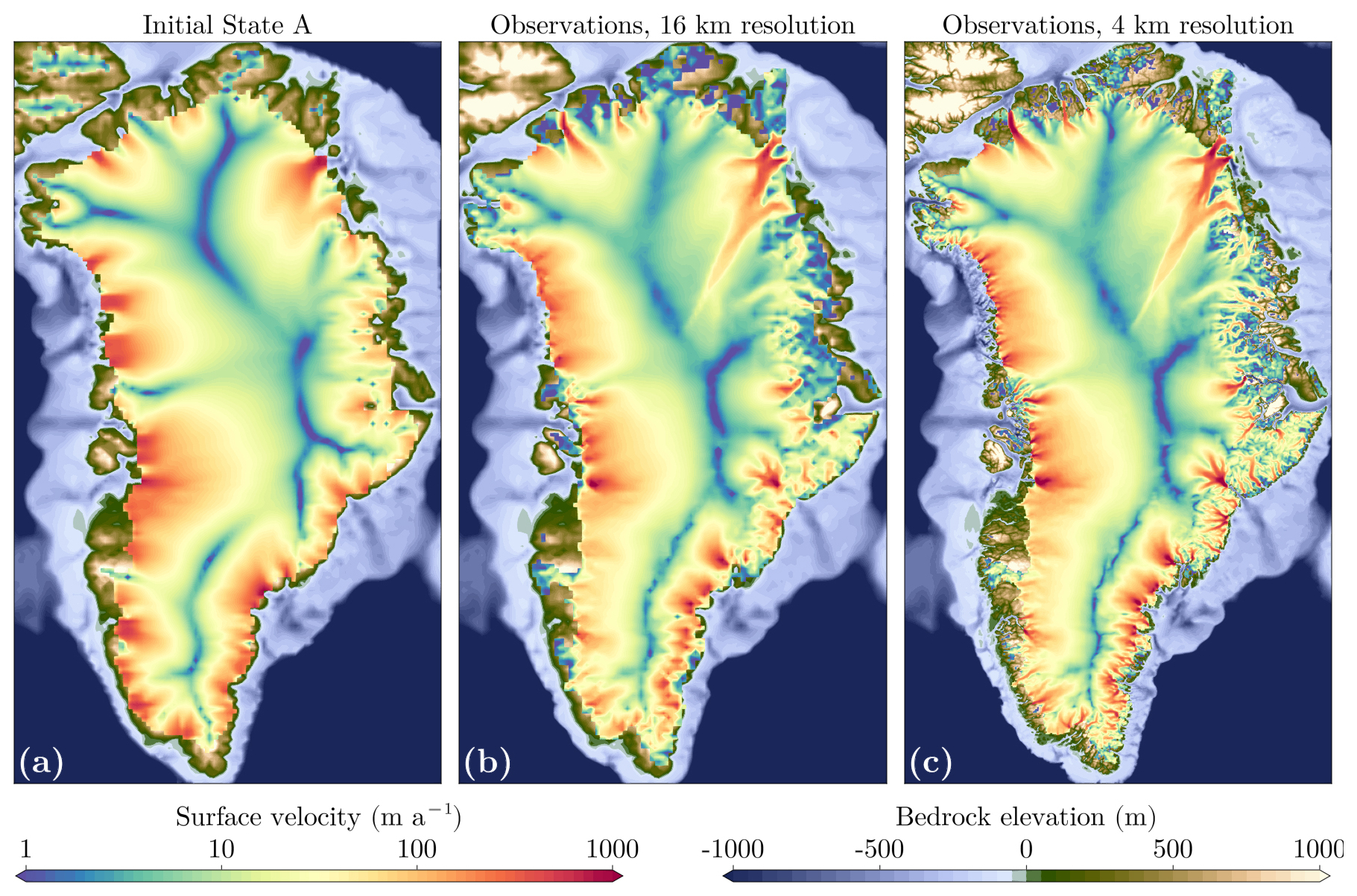
Figure 13 Ice sheet extent and surface velocities for (a) initial condition A used in this study; (b) surface velocity data of Joughin et al. (2018) at 16 km resolution; (c) surface velocity data of Joughin et al. (2018) at 4 km resolution. Panel (a) is the same as Fig. 1b.

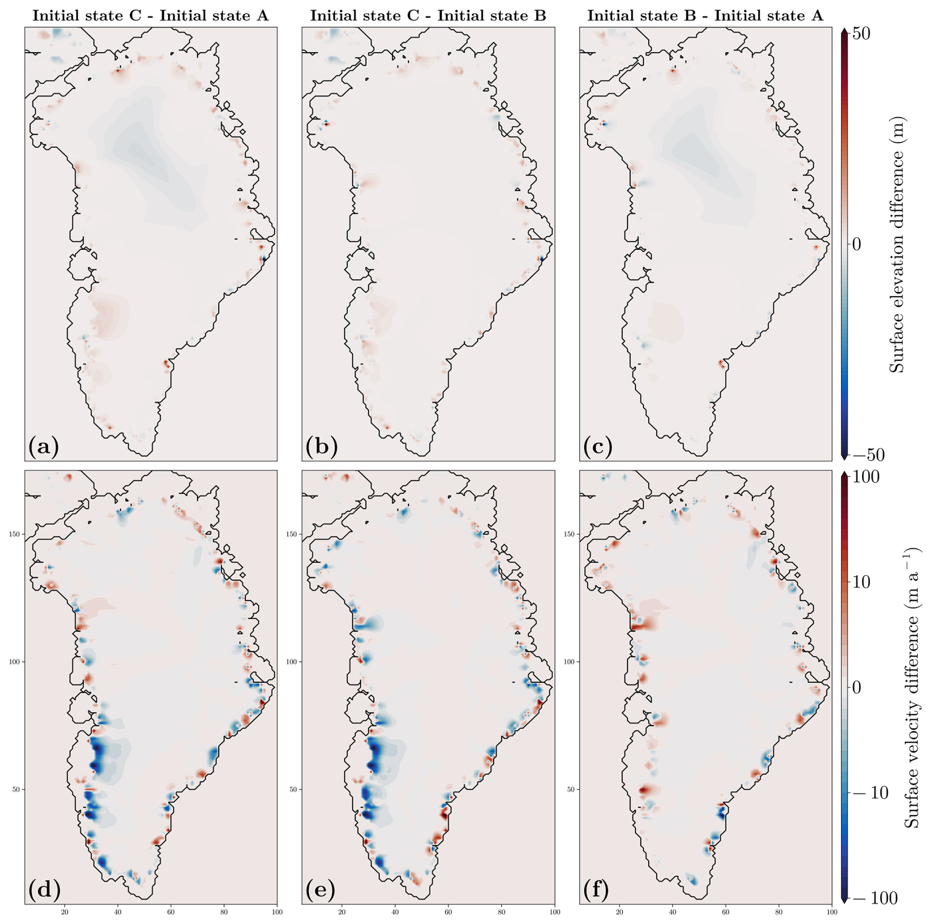
Figure 14 Differences in surface elevation and surface velocity between the three initial states.

Figure 14 shows the difference between the ice thickness and surface velocities between the three initial states A, B and C.

7 Comparison to ice streams in other areas of the GrIS

The variability of the retreated PIS and HIS is unique when comparing them to other ice streams in the model domain. Figure 15 displays the same information as Fig. 8, but with ice streams on the west coast of Greenland in the left-hand-side panels. These glaciers are all in the steady-streaming state, indicated by maximal basal water thickness and a constant, nonzero basal velocity. Very slight variations in the mean ice thickness can be seen, but none so great as for the retreated HIS and PIS glaciers that display build-up/surge variability. Notably, these are marine-terminating glaciers, meaning they experience oceanic forcing that promotes basal melting and therefore steady-streaming.

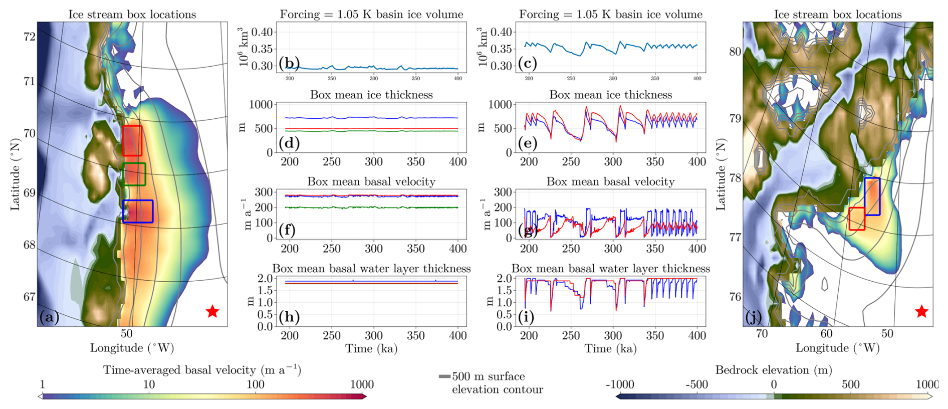
Figure 15 As Fig. 8, but with ice-streams on the west coast of Greenland between 67 and 72° N compared to the retreated PIS and HIS.

Further comparisons can be made to outlet glaciers in the nearby hydrological basin. Figure 16 indicates the variability in marine-terminating glacier along the northwestern coast of Greenland. Most notably, the northernmost glacier displays rapid fluctuations in ice thickness and basal velocity, which accounts for the dominant mode of variability in this drainage basin. These fluctuations occur on a much faster time scale than those of the retreated HIS and PIS, with a period around 2 ka, and much smaller amplitude.

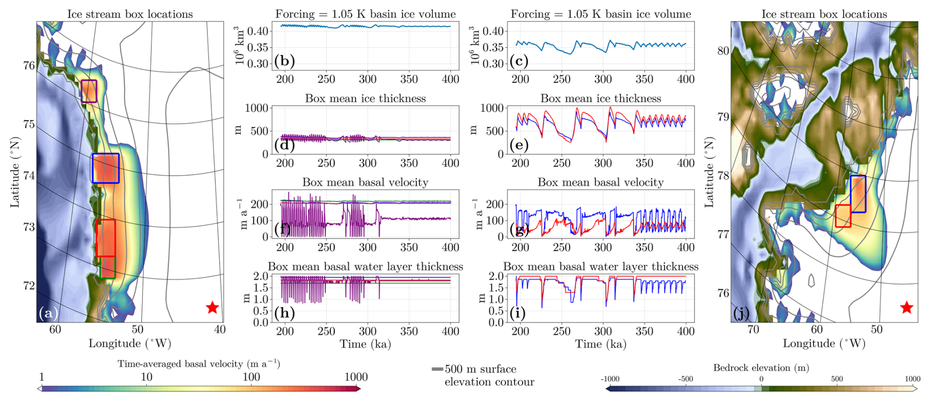
Figure 16 As Fig. 8, but with ice-streams on the west coast of Greenland between 72 and 76° N compared to the retreated PIS and HIS.

Figure 17 shows the variability of other glaciers in the west of the GrIS which are not marine-terminating. These ice streams also experience small fluctuations in basal velocity and ice thickness, but the basal water layer thickness does not notable change as in the retreated PIS and HIS.

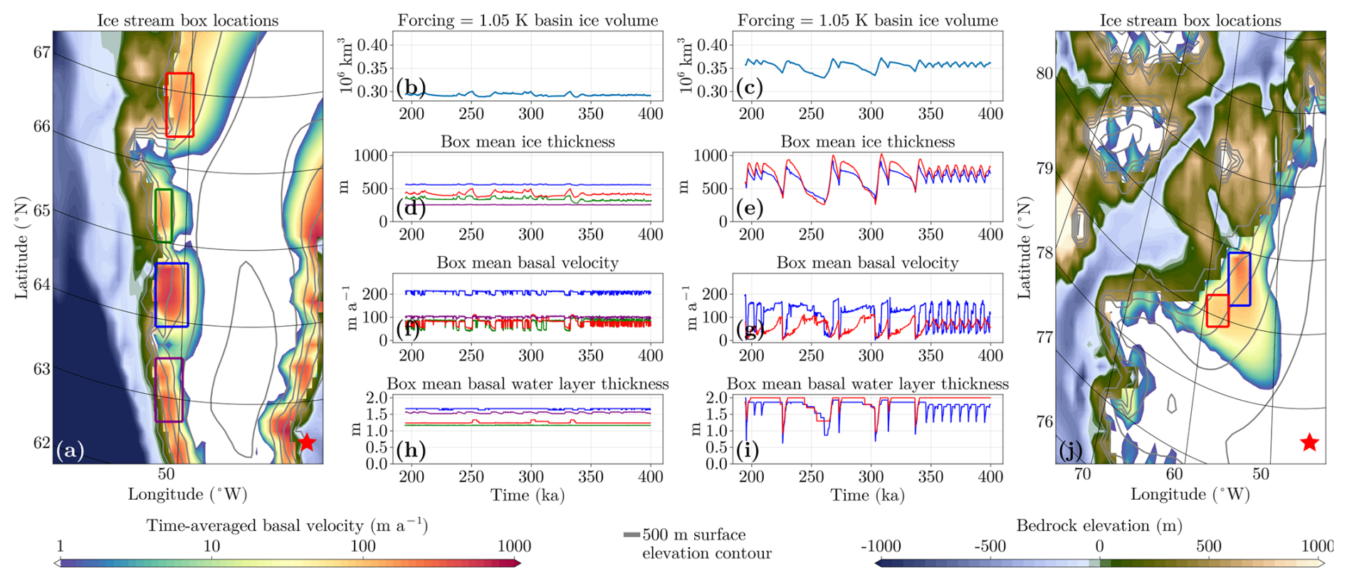
Figure 17 As Fig. 8, but with ice-streams on the west coast of Greenland between 62 and 67° N compared to the retreated PIS and HIS.

8 Comparison to oscillations of the LIS

Large-scale oscillations of ice streams were first proposed as the reason for Heinrich events (HEs) during the last glacial period (LGP) (Heinrich, 1988; Broecker et al., 1992; MacAyeal, 1993), but these events might instead be caused by external forcing (Alvarez-Solas et al., 2013; Bassis et al., 2017). While the variability of the oscillations seen in this study seems similar to the build-up/surge variability seen in most simulations of HEs in the Laurentide ice sheet (LIS) of the LGM (Calov et al., 2002; Hank and Tarasov, 2024; Papa et al., 2006; Roberts et al., 2016; Ziemen et al., 2019; Schannwell et al., 2023), they do not match exactly. Most notably, the Hudson ice stream in those studies displays a more gradual increase in ice volume followed by a sudden surge. This is in contrast to the pattern in the retreated HIS and retreated PIS in this experiment, where the build-up is either over the same time period (in the case of the short oscillations) or faster (in the case of the longer asymmetric events) than the subsequent surge. Additionally, in the latter case, the ice loss accelerates over time, rather than being maximal at the beginning of the surge. It may be the case that the variability seen in the GrIS, while having the same physical mechanism of thermo-mechanical coupling, may have a source additional of variability, e.g. the spatial interaction of the retreated PIS and retreated HIS, that causes it to behave differently from these experiments of a single oscillating ice stream.

Common to ice-sheet model simulations of the LIS are oscillations in ice-sheet volume that sometimes show quasiperiodicity or seemingly chaotic behavior. It would be expected that, due to the large spatial extent of the system and the complex basal topography, the oscillations would not have a near-constant period. Even in the idealized geometry of Calov et al. (2010) there is spontaneous spatial asymmetry that leads to inconsistent oscillatory frequency. Such irregular variability is of special importance when studying the tipping behavior of a system. Still, without an ensemble of simulations starting from similar initial conditions, it is unknown how irregular the variability seen in these studies is.

9 Transient lifetime for a forcing value of 1.05 K

Figure 6a sees a marked difference between the mean ice volume at a forcing magnitude of +1.00 K when compared to those with +1.05 K and greater, suggesting therecould be an “edge state” inhabited by the latter. This edge state would be the chaotic saddle that lies between the stable ice-covered GrIS and collapsed GrIS states. To reinforce the argument that r-tipping does not occur, it would need to be demonstrated that this is not a chaotic saddle. One method is to apply an edge-tracking algorithm that can approximate this non-attracting set (Lucarini and Bódai, 2017; Mehling et al., 2024; Börner et al., 2025), which is the subject of future work.

It can be reasoned that if this were an edge state, the simulations at a forcing magnitude of +1.05 K are also chaotic transients and should eventually tip to an ice-free state, but the lifetime is longer than 400 ka. Using the mean lifetime of the simulations that tip, the critical exponent in Eq. (9) can be estimated. Using a maximum likelihood estimation to fit them to an exponential distribution results in a critical exponent of around γ∼9.959. Using this, the mean tipping time for a trajectory with a maximal forcing of +1.05 K is around 511 ka, which is indeed longer than the 400 ka simulation run time.

A few additional simulations at this forcing level were done going to 1 Ma and are seen in Fig. 18. None of these simulations tip, suggesting that they are not chaotic transients, but rather motion on a genuine chaotic attractor (rather than a ghost) at this parameter value. This further strengthens the argument that the chaotic transients are generated ghost attractor due to crossing a bifurcation point, as this ghost attractor is qualitatively similar to the chaotic attractor that exists before the bifurcation (Lai and Tél, 2011).

Figure 18 Simulations to 1 Ma for a maximal forcing of +1.05 K at three different rates. This simulation time is estimated to be longer than the mean lifetime of a chaotic transient at this forcing value. The temporal resolution of the output of these simulations for the final 800 ka is 5 ka, in comparison to the 200 ka timestep the simulations in Figs. 6 and 8–11

10 Intermediate tipping

Within the simulation ensemble, there are “anomalous” runs that do not behave as the others at their forcing magnitudes. There are two such types: first, for a forcing level of +1.00 K, one simulation ends up in the retreated configuration with ice-volume variability similar to but slightly smaller in magnitude than those of larger forcing values, as seen in Fig. 19. This might suggest the chaotic attractor associated with the ice-stream oscillations also exists for lower forcing values, albeit with a smaller basin of attraction and thus it has a lower probability of being reached.

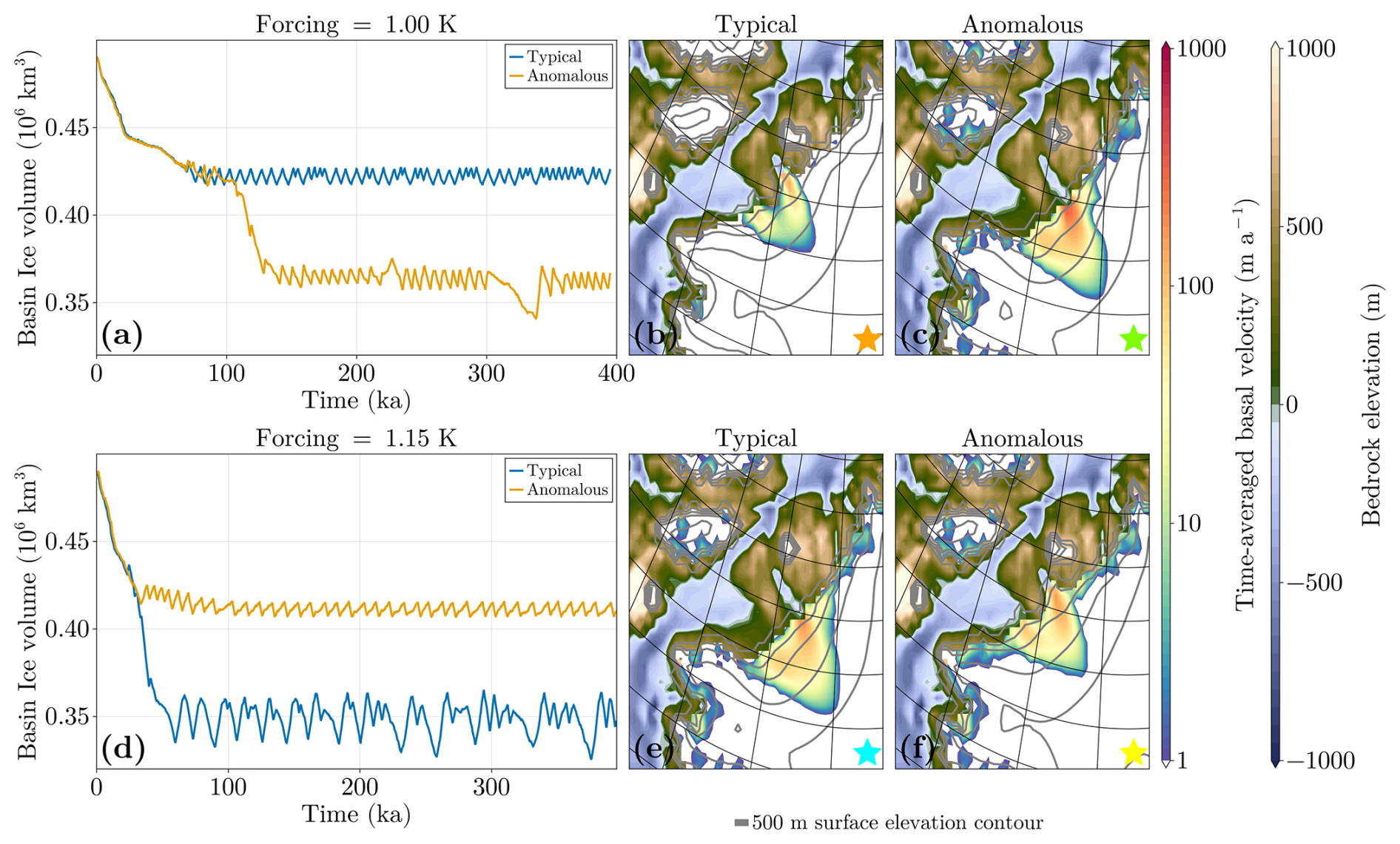
Figure 19 (a) Time series and mean ice thickness for typical and anomalous model trajectories at a forcing of +1.00. (b) Ice sheet extent and time-averaged basal velocity fields of a typical trajectory. (c) Ice sheet extent and time-averaged basal velocity fields of the anomalous trajectory. (d-f) Same as (a–c) but for a forcing of +1.15 K.

Second, there is a simulation with a maximal forcing of +1.15 K that remains in the unretreated configuration. The 1 Ma simulations for a maximal forcing of +1.05 K in Fig. 18 also show the unretreated configuration is possible at this forcing value. In this case, the structure of the attractors may be that there is intermediate tipping similar to Lohmann et al. (2024). This would imply that around a forcing value of +1.00 to +1.05 K, there are two attractors for the ice-covered state, corresponding to the retreated and unretreated configurations. The attractor for the retreated GrIS experiences a bifurcation between +1.05 and +1.10 K, with corresponding chaotic transients remaining on the associated ghost attractor. On the other hand, the attractor of the unretreated GrIS experiences a bifurcation at a forcing value slightly larger than +1.15 K. This scenario could then have r-tipping onto either the unretreated or retreated configurations, the latter of which experiences an earlier tipping to an ice-free state, resulting in an indirect r-tipping to the ice-free state. The basin boundary between the two ice-covered attractors could be fractal, leading to nearby initial conditions approaching one or the other (McDonald et al., 1985).