the Creative Commons Attribution 4.0 License.
the Creative Commons Attribution 4.0 License.
 | 19 Jun 2026
Assessing the impact of the Human Development Index on historical trends in the INFERNO fire model
João C. M. Teixeira
Chantelle Burton
Douglas I. Kelley
Gerd A. Folberth
Fiona M. O'Connor
Richard A. Betts
Apostolos Voulgarakis
Fire schemes within Earth System Models capture long-term historical trends in burnt area, but they struggle to reproduce the pronounced decline observed over the past two decades. This study investigates whether the observed decline in global burnt area during 1998–2016 can be better represented in the JULES-INFERNO fire model by introducing a globally uniform dependence on the Human Development Index (HDI) as a proxy for socio-economic fire controls.
This approach substantially reduces regional biases in annual burned area. In Temperate North America, model bias decreases from +735.57 % to +44.46 %, with similarly large reductions in Central America, Southern Hemisphere South America, Europe, and the Middle East. HDI also improves the representation of burned area trends in eight of the 14 GFED4s regions with significant negative trends in observations. However, correcting large positive regional biases removes compensating errors in the original model, leading to a stronger global negative bias, which shifts from −34.35 Mha in JULES-INFERNO to approximately −111 Mha in JULES-INFERNO with the HDI implementation.
Overall, while HDI improves regional performance and better captures observed downward trends in some regions, it also reduces interannual variability and underestimates larger fires. This highlights both the potential and limitations of representing socio-economic influences within fire models using a simplified globally uniform formulation.
- Article
(10386 KB) - Full-text XML
- BibTeX
- EndNote


Globally, burnt area trends are influenced by complex interactions between climate change, human activities, and natural ecosystem processes, resulting in large climate change and variability over the past few decades. However, the long-term trend (e.g., 1997–2016) has shown an overall decline in global burnt area, especially driven by changes in burnt area of African savannas and grasslands (decline of 1.27 % yr−1 (Andela et al., 2017)). The trend, shown in Fig. 1b), is attributed to changes in land use, particularly agricultural expansion and intensification in savanna and grassland regions, which reduces the availability of fuel for fires (Riley et al., 2019; Andela et al., 2017).
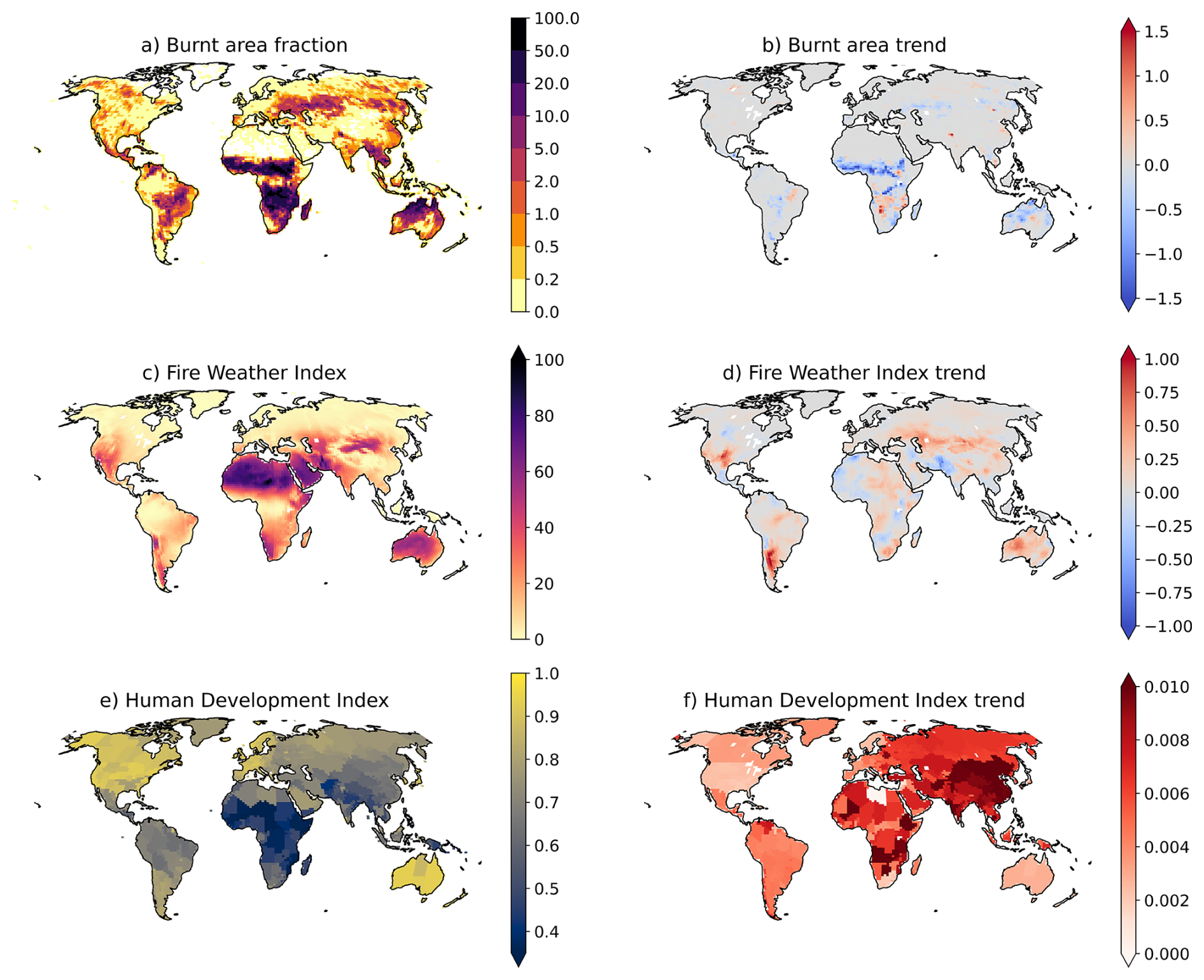
Figure 1Global distribution of (a) Burnt area fraction from the Global Fire Emission Database version 4 (GFED4s) (%) total annual average (1997–2016) and (b) respective trend (% yr−1); (c) Fire Weather Index (FWI) average across 1997–2016 and (d) respective trend (yr−1); (e) Human Development Index (HDI) average across 1997–2016 and (f) respective trend (yr−1). The FWI maps represent long-term climatological averages intended to illustrate broad-scale spatial patterns and trends in fire-conducive conditions.
In addition, fire is also actively used as a land management tool, for example to clear land for agriculture, manage vegetation, and maintain pasture systems, particularly in tropical and subtropical landscapes. Figure 1 illustrates the broad-scale spatial patterns and long-term trends of burnt area, fire weather, and the Human Development Index (HDI).
Climate is a key factor influencing fire activity. Rising temperatures are leading to longer fire seasons, particularly in temperate and boreal regions (Sullivan et al., 2022; Jones et al., 2024). Reduced rainfall during the fire season increases the likelihood of large fires, while increased rainfall can enhance vegetation growth and fuel availability. However, while climate strongly influences inter-annual variability and long-term trends, particularly in temperate and boreal regions, human activity – such as land use change, agricultural expansion, and fire suppression – has been the dominant driver of long-term declines in global burnt area, especially in tropical savannas (Riley et al., 2019; Andela et al., 2017; Marlon et al., 2008).
Furthermore, human population density and prosperity significantly influence burnt area. (Andela et al., 2017) show that population growth and socioeconomic development, driven by increased demand for agricultural products, have led to a shift towards more capital-intensive agriculture and reduced fire use. These factors produce a strong inverse relationship between burnt area and economic development.
In Coupled Model Intercomparison Project frameworks, fire processes are generally represented through simplified global-scale schemes linking burnt area to vegetation, fuel availability, and climate conditions. These models typically include lightning and human ignitions, as well as representations of flammability and fuel continuity, but do not resolve fine-scale processes such as local suppression, management practices, or sub-grid fuel heterogeneity (Yue et al., 2014; Rabin et al., 2017).
However, CMIP6 Earth System Models (ESMs) (Eyring et al., 2016) do not reproduce the observed decline in global burnt area and fire carbon emissions over recent decades, largely due to an underestimation of anthropogenic fire suppression (Li et al., 2024). This is consistent with Forkel et al. (2019), who show that fire activity is strongly sensitive to both climate and socio-economic drivers, highlighting the need for improved representation of human influences in fire-enabled models.
Moreover, key human-driven factors – such as agricultural expansion, land-use change, fire management policies, and landscape fragmentation, have substantially reduced fire activity, particularly in tropical savannas (Andela et al., 2017; Forkel et al., 2019). These processes are not adequately represented in most CMIP6 models, contributing to an overestimation of burned area and associated fire carbon emissions.
Most global fire models, such as JULES-INFERNO (Mangeon et al., 2016; Burton et al., 2019), represent human ignitions using simple functions of population density, typically increasing up to a threshold beyond which additional population has no effect (Rabin et al., 2017; Teckentrup et al., 2019; Ford et al., 2021). This approach does not represent the influence of socio-economic factors on ignition and suppression, nor does it capture regional variability in contemporary burning practices.
This limitation affects the realism of climate and carbon cycle projections and highlights the need to better represent dynamic human influences on fire regimes, including evolving socio-economic conditions such as population growth, infrastructure development, and fire management strategies (Li et al., 2024).
In current global fire models, changes in fire activity are typically quantified through a separation of climate-driven controls – such as fire weather, fuel moisture, and vegetation productivity – and anthropogenic influences, commonly represented using simplified proxies such as population density or land-use change. This structural separation strongly influences how models attribute historical and future changes in fire activity to climate and human drivers (Burton et al., 2024), and can lead to substantial differences in simulated fire responses when anthropogenic processes are under-represented.
Fire is also a key component of the climate system through two-way feedbacks, affecting atmospheric composition, surface albedo, and land–carbon exchanges, while being itself sensitive to changes in fire weather, fuel availability, and ignition conditions. Recent work (Verjans et al., 2025) shows that improved fire representations can substantially alter simulated climate responses, highlighting the importance of realistic fire modelling within ESMs.
HDI combines four indicators: life expectancy at birth, expected and mean years of schooling, and Gross National Income (GNI) per capita (Bhanojirao, 1991). These are normalised and aggregated as the geometric mean of life expectancy, education, and income dimensions. It has been widely used to study socio-economic influences on the Earth System, including links between development and environmental pressure (Türe, 2013), the decoupling between human development and resource use or emissions (Hickel, 2020), and the role of socio-economic development pathways in shaping sustainability outcomes at regional and global scales (Roy et al., 2023).
Chuvieco et al. (2021) shows that HDI is strongly correlated with inter-annual variability in burned area, with higher HDI regions exhibiting lower variability due to mechanisation and reduced reliance on fire in agriculture, while lower HDI regions show greater variability linked to continued use of fire for land management. Incorporating socio-economic indicators such as HDI therefore improves the ability of fire models to reproduce observed variability patterns.
More recently, Perkins et al. (2024) introduced WHAM! (the Wildfire Human Agency Model), a global behavioural, geospatial model designed to represent human fire use and management in a form that can be coupled to dynamic global vegetation models, demonstrated via coupling with JULES-INFERNO. WHAM! is empirically grounded in a global synthesis of anthropogenic fire impacts and seeks to move beyond single-proxy parametrisations by representing underlying behavioural and land-system drivers that shape how people ignite, manage, and suppress fires across regions. As such, WHAM! constitutes a more sophisticated, process-oriented attempt to incorporate anthropogenic drivers in fire modelling. In contrast, the HDI-based implementation in this work is intentionally simplified to remain tractable for ESM applications.
Additionally, Li et al. (2013) and Zou et al. (2019) investigated the use of Gross Domestic Product (GDP) to parametrise human influences on fire activity. While these approaches capture broad relationships between economic development and fire occurrence, they offer a limited representation of the underlying socio-economic processes that govern fire ignition and suppression.
Human influences on fire activity have become increasingly pronounced since the late 18th century, driven by industrialization, land clearance, population growth, and the evolution of fire management practices (Bowman et al., 2020). These trends highlight the need for improved representation of socio-economic factors in fire models to better quantify human–fire interactions, including aspects such as socio-economic conditions and historical and institutional context. This is particularly important as the impacts of vegetation fires are expected to intensify under anthropogenic climate change (Sullivan et al., 2022; Jones et al., 2024; Haas et al., 2024).
Socio-economic and policy factors also play a key role in shaping fire regimes. For example, changes in wildfire governance and policy learning can alter perceptions of fire risk and management strategies (Nikolakis and Roberts, 2022), while global studies show that variations in fire management policies have contributed to long-term reductions in fire occurrence and burned area (Pandey et al., 2023).
Several studies indicate that, in developed regions, fire occurrence and impacts are strongly shaped by governance and policy, rather than individual behaviour alone. For example, changes in policy and governance have been shown to influence fire outcomes (Nikolakis and Roberts, 2022), while risk framing and coordination efforts also play an important role (Jacobson et al., 2022). Modelling approaches that emphasise management institutions further highlight the significance of governance in shaping fire dynamics (Ford et al., 2021). Observed reductions in fire numbers or size following prevention and suppression policy shifts provide additional empirical support (Curt and Frejaville, 2018), and studies demonstrate that policy design and its dependence on local stakeholder and contextual factors can determine effectiveness (Carreiras et al., 2014). Finally, institutional capacity and spending have been linked directly to fire outcomes, underscoring the importance of resources and coordination (Mourão and Martinho, 2014).
Notably, Curt and Frejaville (2018) found that wildfire policies in Mediterranean France have led to a nearly linear decrease in the number of fires since 1975, though the burnt area has fluctuated more abruptly. Therefore, representing land and fire management policies in global fire models is crucial to building confidence in the modelling frameworks which are used to understand future climate regimes. This, in turn, can underpin decision-making by policy-makers in regards to fire policy in the future.
Socio-economic factors impact on fire are complex and depend on factors that are difficult to represent in an ESM context, including government policy and cultural behaviour, which vary widely across regions. As a result, current climate-ESM formulations do not fully capture these processes.
Rather than attempting to represent the full complexity of socio-economic influences, this study uses a simplified emergent relationship based on HDI as a proxy, which is more suitable for large-scale applications. Here, fire suppression broadly represents human actions that limit fire spread, including containment and land management practices, whose effectiveness varies with regional resources and infrastructure. Processes such as fine-scale suppression tactics, planned burning, fuel management, and weather-driven fire extinction are not explicitly represented. We use observed HDI, burnt area, and Fire Weather Index (FWI) datasets to derive the HDI-burnt area relationship and implement this in the INFERNO fire model.
In Sect. 2, we explore the relation between HDI and burnt area and describe the INFERNO fire model, the coupling of INFERNO to the latest representation of the land surface model (JULES-ES) as used in the UK's Earth System Model (UKESM1), and how we include HDI into INFERNO's ignition scheme. In Sect. 3, we evaluate the impact of considering HDI on burnt area, burnt area trends, as well as the impact of external model drivers of burnt area trends. Discussion and conclusions from this work are presented in Sect. 4, where we focus on novel model results, placing the link between socio-economic factors and fires in context with existing literature. Model limitations and known issues are also highlighted.
2.1 Observed Datasets
2.1.1 The Human Development Index dataset
HDI originated from the annual Human Development Reports created by the United Nations Development Programme (UNDP) Human Development Report Office. These reports had the explicit purpose of shifting the focus of development economics from national income accounting to people-centred policies. The aim was to provide a simple composite measure of human development to convince the public, academics, and politicians to evaluate development not only by economic advances but also improvements in human well-being. HDI serves as a crucial metric for assessing the development status of regions globally, and it has been used in several studies to better understand the socio-economical impacts in the Earth System (ES) (Türe, 2013; Hickel, 2020; Roy et al., 2023).
HDI is a composite index (ranging from zero to one) measuring four key metrics (Bhanojirao, 1991):
-
life expectancy at birth
-
expected years of schooling
-
average years of schooling
-
gross national income (GNI) per capita
These metrics are then normalised by their respective maximum value, and HDI is calculated as the geometric mean of life expectancy, education, and GNI per capita, as shown in Eq. (1).
where HN is the normalised life expectancy, EN is the normalised arithmetic mean of the two education indices and IN is the normalised GNI per capita.
The work conducted by Kummu et al. (2018) introduces gridded global datasets for Gross Domestic Product (GDP) and Human Development Index (HDI), covering a 25-year period from 1990 to 2015 with annual frequency and a spatial resolution of 5 arcmin. This temporal coverage and high-resolution global scope enable comprehensive analyses of trends, patterns, and changes in HDI across diverse regions and timescales.
To produce these datasets, Kummu et al. (2018) employed a comprehensive approach. The HDI dataset was compiled by initially constructing a full national HDI dataset based on data from the Human Development Reports by UNDP. For countries not included in the UNDP reports, independent data sources were utilized, and for missing or outdated data, a methodology involving scaled regional data was adopted.
2.1.2 Burnt Area observation
Global Fire Emission Database version 4 (GFED4s) is a long-running, operationally updated dataset used globally for fire and emissions research. While the core methodological reference (Giglio et al., 2013) describes the development of the GFED4s framework, the dataset itself has been continuously updated to include fire emissions up to recent years (e.g., including 1997–2016).
We use data from the GFED4s to understand the relation between HDI and burnt area, as well as to assess the model performance in simulating burnt area. This dataset is provided as a gridded product at a 0.25° resolution. It is derived from a multi-sensor satellite dataset, including satellite data based on active fire detection, and including small fires based on statistical modelling, as detailed in (Randerson et al., 2012).
We apply regions defined in the GFED4s dataset to the modelled data to evaluate the results at a regional level (Fig. A1).
2.1.3 Fire Weather Index
The Canadian FWI is a component of the Canadian Forest Fire Danger Rating System (CFFDRS) and provides a numerical rating of fire intensity based solely on weather conditions (temperature, relative humidity, wind speed, and precipitation). Although it was originally developed for Canadian boreal forest conditions, the FWI system is not region-specific and has been successfully applied in diverse ecosystems worldwide, including in Europe, South America, Australia, and parts of Africa and Asia. Its broad adoption stems from its simplicity, weather-based formulation, and scalability (Field et al., 2015).
The work developed by Vitolo et al. (2020) provides an ERA5-based global meteorological wildfire danger dataset based on the Global ECMWF Fire Forecast (GEFF) model and the ERA5 reanalysis.
In this dataset, the FWI is calculated using meteorological variables (e.g., temperature, humidity, precipitation, and wind speed) from the ERA5 reanalysis dataset. To accurately represent wildfire conditions at local noon, when fire danger is typically highest, atmospheric fields from ERA5 undergo preprocessing, stitching together hourly forecasts, ensuring that meteorological conditions are representative of 12:00 noon local time around the world.
The GEFF model, calculates the FWI by modelling fuel moisture response to atmospheric forcing at different depths. Three fuel moisture levels are used, representing surface fuels, deeper organic material, and compact fuels, each responding at different rates to changes in weather. These fuel moisture levels are then combined to estimate fire behaviour, such as the rate of spread and fire intensity, providing a comprehensive fire danger index.
The GEFF-ERA5 FWI reanalysis dataset, available from 1979 onwards at a spatial resolution of 28 km, was used in this study with monthly averaged values.
When comparing datasets (modelled or observed) at different grid resolutions, the higher-resolution dataset is re-gridded to the lowest-resolution grid using a first-order conservative area-weighted re-gridding method.
2.2 Relation between HDI and Burnt Area
As climate is a dominant factor influencing fire activity, it is essential to first account for and remove the long-term trend component associated with changing fire-weather conditions before exploring the effects of socio-economic factors on burnt area. For this, and considering that the FWI depends solely on the weather variables that drive fire activity, we perform a FWI-trend adjustment procedure at each individual grid cell.
For each grid cell (i,j), we consider the monthly time series (t) of FWI, FWIi,j(t), and burnt area, BAi,j(t). Both are normalised over the study period using min-max scaling, defined as , where X∈ FWI,BA.
To estimate the FWI-associated trend component in the time series of burnt area, we first fit a linear regression of the normalised FWI time series against time, , to capture the temporal trend in fire-weather risk. We assume that the long-term evolution of fire-weather conditions can be approximated by a linear temporal trend over the study period. Independently, we fit a linear regression to the normalised burnt area time series as a function of time to obtain its intercept, which serves as a baseline level for the trend construction.
We assume that changes in burnt area associated with long-term variations in fire-weather conditions can be represented as a first-order linear component consistent with the temporal trend observed in FWI. This assumption allows us to construct a simplified representation of the climate-related trend in burnt area, which is then isolated and removed from the total signal. The FWI-associated trend component of burnt area is estimated as:
Finally, the FWI-associated trend component is removed from the normalised burnt area time series while preserving the original mean:
where is the temporal mean of the estimated FWI-associated trend component at each grid cell.
This results in a revised time series of burnt area in which the long-term trend component associated with FWI has been reduced (FWI-trend adjustment). It will be subsequently used to analyse how socio-economic factors impact fire activity through the use of HDI.
Importantly, this procedure removes only the long-term trend component associated with FWI and does not remove interannual or short-term weather variability. Consequently, the adjusted burnt-area series retains year-to-year variability while reducing the long-term component associated with changing fire-weather conditions.
We further assume that residual long-term variations in burnt area after FWI-trend adjustment primarily reflect the influence of socioeconomic factors. We note, however, that fuel availability and continuity can also be important determinants of fire activity and may influence burnt area trends even after the FWI-trend adjustment.
To ensure consistency across our burnt area results, we define the burnt area fraction as the proportion of each grid cell that burns in a given year, calculated as the burned area divided by the total cell area (Giglio et al., 2013).
Figure 2 shows the spatial correlation coefficients between FWI and FWI-trend adjusted burnt area (panel a), and between HDI and FWI-trend adjusted burnt area (panel b). Overall, correlations are spatially variable but are predominantly not statistically significant across most regions of the globe. Where statistically significant relationships do emerge, the correlation between HDI and FWI-trend adjusted burnt area is generally negative and tends to be stronger than that with FWI. The negative relationship is particularly evident over Eurasia, Central Africa, and Eastern and Western Australia, where increases in FWI coexist with regional decreases in burnt area that are significantly correlated with HDI (Figs. 1 and 2). Nonetheless, the FWI-trend adjusted burnt area shows a strong positive correlation with FWI over the boreal regions of North America and Siberia, as well as the Cerrado ecoregion of South America.
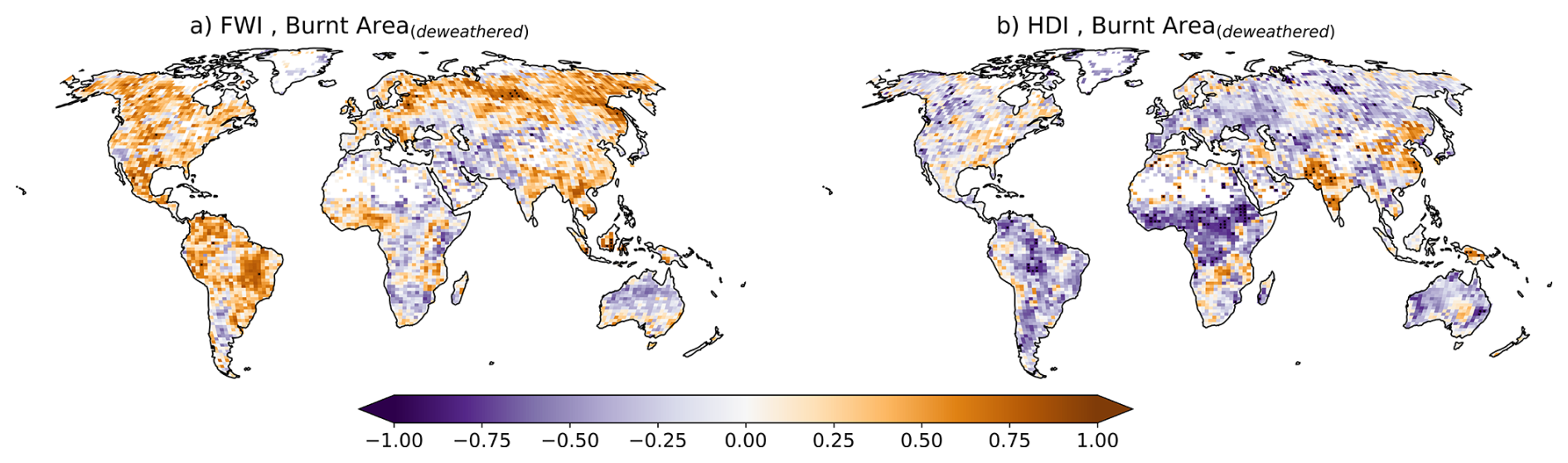
Figure 2Pearson correlation coefficient between the monthly mean (1997–2016) (a) FWI and the FWI-trend adjusted Burnt Area (GFED4s), and (b) HDI and the FWI-trend adjusted Burnt Area (GFED4s). Stippling indicates grid points where the Pearson correlation is statistically significant at the 5 % level after controlling for the false discovery rate using the Benjamini and Yekutieli (2001) procedure.
Multiple techniques are used to further investigate the relationship between HDI and burnt area. The scatter plot of the FWI-trend adjusted burnt area against HDI in log-space is presented in Fig. 3. Due to the inherent stochasticity of burnt area, the results show a wide range of values, spanning small to large relative burnt area fractions for any given HDI. To account for this variability and isolate the effects of HDI on burnt area, we applied a Bayesian Linear Regression method (Klauenberg et al., 2015) to the log-transformed burnt area fraction, denoted by log (BA*):
where c represents the expected value of log (BA) at HDI =0, m represents the change in log(BA) with HDI, and ) represents the residual error. The FWI-trend adjusted burnt area, BA*, is expressed as a fraction (0−1) prior to log-transformation.
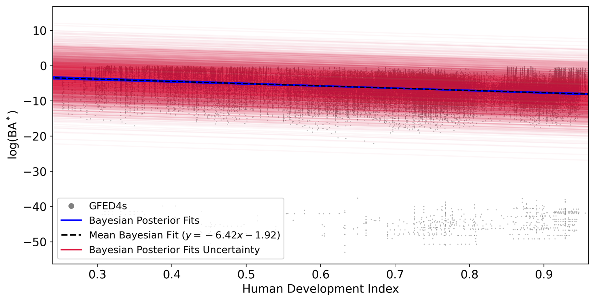
Figure 3Bayesian linear regression performed in log-space on log (BA*) with HDI as predictor. The grey dots represent the scatter plot of all monthly burnt area values at all grid cells as a function of HDI in the log-space. The blue solid lines represent posterior predictive samples of the fitted regression. The black dashed line represents the posterior mean fit. The red lines indicate the uncertainty envelope derived from the posterior predictive distribution. The regression results are shown in log-space.
We assume that log (BA*) is normally distributed centred on the linear predictor, with residual standard deviation σ treated as an additional parameter. Priors for the regression coefficients were chosen to be weakly informative, with BA, , and σ∼ HalfNormal(25).
This formulation allows both positive and negative relationships between HDI and burnt area, while the log-transformation ensures that predicted burnt area remains strictly positive when interpreted in natural space.
The model was fitted using monthly burnt area and HDI data from all grid cells, allowing short-term variability to be smoothed and the longer-term relationship between HDI and burnt area to be quantified. Posterior inference was carried out using the No-U-Turn Sampler (NUTS) implemented in the PyMC Python package (Kelley et al., 2019). Convergence was verified via R-hat values <1.01, and 1000 posterior draws were generated to quantify parameter uncertainty.
To visually represent the uncertainty, 145 posterior draws were plotted as solid blue lines in Fig. 3. This number was chosen pragmatically to provide a sufficiently large sample size to capture posterior variability while avoiding excessive clutter in the figure, ensuring a clear representation of both the spread and central tendency of the predicted relationship between HDI and burnt area.
This method shows that the observations show a linear decline in burnt area with increasing HDI, with a posterior mean slope of −6.42.
2.3 INFERNO fire model
In this work we simulate fire using the INFERNO (INteractive Fires and Emissions algoRithm for Natural envirOnments; Mangeon et al. (2016)) fire model. INFERNO uses an approach based on Pechony and Shindell (2009), adapted to allow interactions within an ESM framework. More precisely, INFERNO uses water vapour pressure deficit as one of the main indicators of flammability and an inverse exponential relationship to relate flammability to soil moisture.
where IT represents the fire ignitions, including natural and human ignitions as well as fire suppression by humans, FPFT the flammability per PFT dependent on the 1.5 m temperature, 1.5 m relative humidity and fuel density – as defined in Eqs. (4)–(6) from Mangeon et al. (2016) – and is the average burnt area for each model Plat Functional Type (PFT).
The burnt area, represented in Eq. (5), is the average burnt area per fire for each model PFT. This decouples fire spread from localised effects of wind or topography, which are not resolved at the coarse spatial scales used in ESMs. Instead, INFERNO relies on PFT-specific flammability and fire occurrence metrics, capturing broad-scale, climate and vegetation-driven fire dynamics. This approach does not explicitly represent sub-grid heterogeneity in topography or local meteorology, which is a limitation that may influence local fire spread.
It should be noted that the recent work by Haas et al. (2022) shows that topography and wind speed have an impact on fire size even when aggregated to a 0.50° grid cell scale. However, the resolution of the model used in this study is coarser – approximately 1.75°.
INFERNO fire ignitions are split into Natural Ignitions (IN) from cloud to ground lightning flashes and from Human activities (IA) dependent on population density (PD) as described in Eq. (6). Humans are also responsible for suppressing fires in the model, using a suppression function (fNS) dependent on human population density (Eq. 7) to represent the fraction of fires not suppressed by humans. The total ignitions (IT) are represented by Eq. (8).
where is a function that represents the varying anthropogenic influence on ignitions in rural versus urban environments, and the parameter α=0.03 represents the number of potential ignition sources per person per month per km2, and HDI represents the Human Development Index.
In Eq. (7) the fraction of fires that remain unsuppressed at the most populated areas is expressed by c1. The maximum number of fires that remain unsuppressed at the distant, unpopulated regions is defined by the sum of c1 and c2, and the rate at which the number of unsuppressed fires decreases with increasing population density is determined by ω. As expressed by Pechony and Shindell (2009), due to the lack of global quantitative data, constant values are selected in a rather heuristic manner: c1=0.05, c2=0.9, and ω=0.05. In this way, up to 95 % of fires are assumed to be suppressed in densely populated regions, and 95 % are assumed to remain unsuppressed in unpopulated regions.
Previously, INFERNO only included information on population density. To represent the socio-economic factors impacting fire ignition and suppression, we include a HDI term (1− HDI) in our human ignition and suppression Eqs. (6) and (7) (shown in bold). In addition it should be noted that the HDI implementation scales both c1 and c2 according to the HDI value of any given grid point.
This approach does not directly implement the empirical relationship established from observational data in Sect. 2.2. Instead, it introduces an HDI dependent formulation based on the assumption that ignition rates decrease and suppression increases with higher HDI. This reflects the hypothesis that more developed regions experience fewer ignitions and greater fire control capacity. We then test whether this indirect implementation can reproduce the observed relationship between burned area and HDI.
Despite being a simple representation, it aligns with the few studies found in literature that looked at the impact governmental policies have on prevention of wildfires (e.g., the work by Curt and Frejaville (2018)). Furthermore, although the equations used could be adjusted to provide the best results, we avoid this approach in this first implementation in INFERNO to avoid masking compensating biases that are existent or could arise from this implementation.
In this representation of socio-economic impacts on fire ignition and suppression, we assume that fire ignitions decrease and fire suppression increases for areas with more effort in human development improvements. Moreover, it reduces the impact changes in population density have in areas with high HDI while keeping a dependency on population density changes for areas with low HDI, where policies on land and fire management have a greater role than other human behaviours in controlling ignitions (Nikolakis and Roberts, 2022; Ford et al., 2021; Jacobson et al., 2022; Carreiras et al., 2014; Mourão and Martinho, 2014). The impact of HDI on INFERNO anthropogenic fire ignitions and suppression, represented as IA (Eq. 6) and fNS (Eq. 7) respectively, is depicted in Fig. 4.
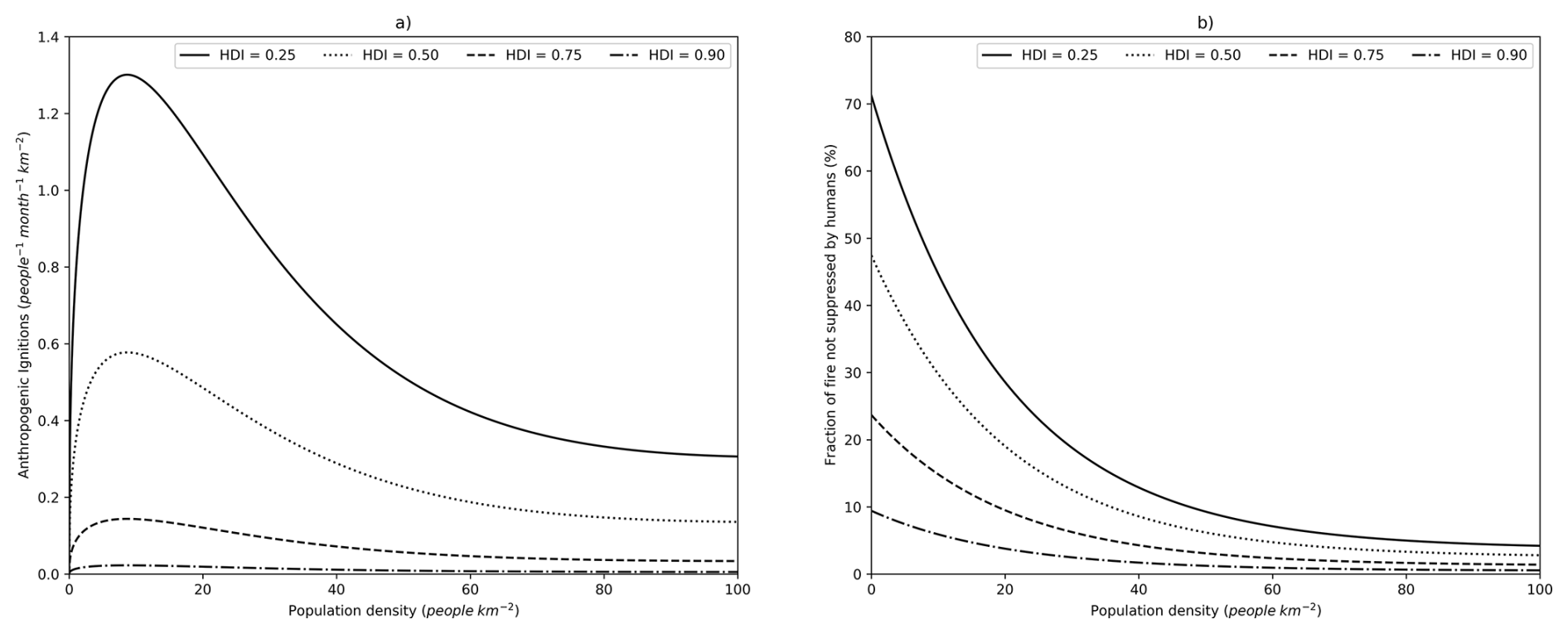
Figure 4Anthropogenic fire ignitions (people−1; per month; km−2) (a) and fraction of fire not suppressed by humans (%) (b) as a function of population density (people; km−2) and Human Development Index.
We obtained HDI data from the gridded global datasets for Gross Domestic Product and HDI (Kummu et al., 2018), which provides HDI data from 1990 to 2015. To cover the full modelled period (1860–2016), the HDI data is linearly ramped from the minimum HDI value of the dataset (0.2) to its value in 1990 for each grid point. The original HDI dataset was spatially interpolated using a nearest-neighbor interpolation method to match the model grid, and was updated at the same frequency as the original dataset – annually.
2.4 JULES-ES and INFERNO
We use the community land surface model JULES (Joint UK Land Environment Simulator; Clark et al. (2011); Best et al. (2011)) at version 5.7, with the science configuration of the land surface as used in UKESM1 (Sellar et al., 2019a), including 13 PFTs, and dynamic vegetation from TRIFFID (Top-down Representation of Interactive Foliage and Flora Including Dynamics; Cox et al. (2000); Cox (2001)). This ES configuration of JULES is known as JULES-ES (Mathison et al., 2022). JULES simulates surface fluxes of water, energy, as well as vegetation and carbon. Here, we use JULES as a stand-alone offline model run at a spatial resolution of N96 (equivalent to a horizontal resolution of 135 km in the mid-latitudes). The Climate Research Unit – National Centers for Environmental Predictions reanalysis (CRU-NCEP v7) (Harris et al., 2014; Viovy, 2018) atmospheric variables are provided at 6 h intervals to drive JULES, including carbon dioxide (CO2), precipitation, temperature, specific humidity, wind, air pressure, and short and long wave radiation. The model runs from 1860–2016 with this forcing. In this work, we analyse the period that overlaps with observations (1997–2015).
We use the fire–vegetation coupling described in Burton et al. (2019, 2020), which incorporates additional carbon cycle feedbacks from litter and vegetation burning and explicitly accounts for fire-induced mortality by plant functional type (PFT). Mortality rates, set to 40 % for trees, 60 % for shrubs, and 100 % for grasses, are based on literature values and the methodology documented in Burton et al. (2019), which includes a comprehensive evaluation of the model performance in representing the evolution of vegetation within the context of JULES-INFERNO model. This setup differs from that used in Teixeira et al. (2021), which did not include fire–vegetation feedbacks. While simplified, these PFT-specific mortality parameters are intended to capture large-scale patterns of fire-driven vegetation change rather than site-specific fire regimes.
This approach represents a simplification of real-world fire processes. Due to spatial resolution and computational constraints, global fire modelling frameworks necessarily abstract the diversity and complexity of fire behaviour across ecosystems, and variations in fuel type, structure, and landscape heterogeneity are not fully resolved at the model scale. Despite these limitations, coupling with JULES allows INFERNO to capture broad spatial and temporal patterns in fuel availability consistent with large-scale vegetation dynamics and meteorological conditions.
Fire ignitions are based on population density data from HYDE 3.2 (Klein Goldewijk et al., 2017); (Goldewijk et al., 2017) and monthly lightning flash climatology from LIS–OTD (Lightning Imaging Sensor–Optical Transient Detector; Cecil (2006)) observations over 1995–2014, regridded from 0.5° resolution to N96 (1.25 % latitude × 1.875 % longitude). The LIS-OTD climatology provides total lightning flash density (including both intra-cloud and cloud-to-ground flashes); following Christian et al. (2003), total lightning flashes are converted to cloud-to-ground flash density using an empirical partitioning based on observed global relationships between total and cloud-to-ground lightning. After spinning up the model to equilibrium, we complete a full historical simulation from 1860–2019 at N96 and use results from the present day period (1997–2015) for our analysis, which are compared against available observations of burned area.
We performed two model experiments to test the impact of representing the socio-economic factors on fire ignition and suppression in INFERNO. A control experiment referred to as JULES-INFERNO, and a similar experiment, representing the socio-economic factors through HDI on fire ignition and suppression parametrisation described in Sect. 2.3, referred as to JULES-INFERNO+HDI. Figure 5 presents the regridded HDI as provided to JULES-INFEERNO+HDI.
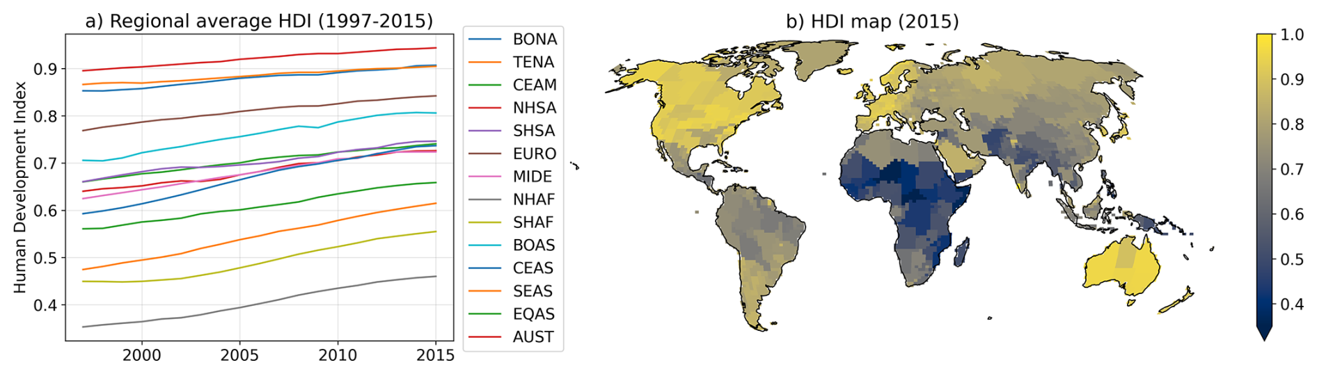
Figure 5Regridded HDI as provided to JULES-INFEERNO+HDI. (a) regional average for the 1997–2015 period and (b) spatial distribution for the year 2015. The regions depicted in (a) are described in Fig. A1.
Socio-economic impacts on fire are not represented in the initial formulation of INFERNO described in Mangeon et al. (2016) for the ignitions and suppression of fires, which affects the values used in the initial implementation of INFERNO. Posterior work by Andela et al. (2019) shows that average burnt area values can be larger than the ones used in the work of Mangeon et al. (2016).
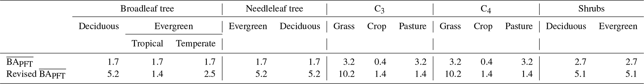
When the HDI-based parametrisation of socio-economic impacts on fire is included in INFERNO, it reduces ignitions and suppression of fires. Therefore, the values of are adapted to align with those reported by Andela et al. (2019). This was achieved by deriving the PFT-specific values by matching those reported by Andela et al. (2019) to the PFT categories represented in JULES as much as possible. These are not direct comparisons and a balance between the PFT representation of the region in JULES was used to estimate a reasonable average burnt area for INFERNO. The values in both experiments are detailed in Table 1.
Table 1Biomass burning average burnt areas (km2; fire−1) for all JULES plant functional types used in this configuration. Based on Burton et al. (2019) (top row) and adapted from Andela et al. (2019) (bottom row).
Although INFERNO has been used in other studies to estimate fire-related emissions, this manuscript focuses exclusively on assessing the influence of the Human Development Index (HDI) on fire activity and on evaluating model performance in simulating burned area fractions. Fire emissions are therefore not analysed in this study.
3.1 Representing Burnt Area – HDI relationship in INFERNO
The posterior fit distributions of the Bayesian Linear Regression parameters slope, intercept and sigma (residual variability caused by none HDI drivers) in Figs. 3 and 7 show narrow intervals for the posterior parameters, evidence of high confidence in the fit for a linear relationship between HDI and FWI-trend adjusted burnt area fraction, with the mean Bayesian fit (dashed black line) presenting a slope of −6.42, and intercept of 19.42 (%).
In summary, this analysis reveals a strong relationship between the HDI and burnt area (Fig. 7). It demonstrates a predominantly negative correlation between HDI and FWI-trend adjusted burnt area globally, and especially in Eurasia, continental North America, central Asia, Southern Africa, and Australia, where increases in FWI have not translated into higher burnt areas (Fig. 2). Conversely, positive correlations persist in regions like the boreal areas of North America, Siberia, and the Cerrado of South America. This evidence suggests that HDI can regionally capture part of the variability in burned area, reflecting some influence of socio-economic factors.
To evaluate the use of HDI as a proxy for representing socio-economic factors influencing fire ignition and suppression in INFERNO, the methodology described in Sect. 2.2 was applied, and the results are presented in Fig. 6, and the distribution of its posterior fits can be found in Fig. 7.
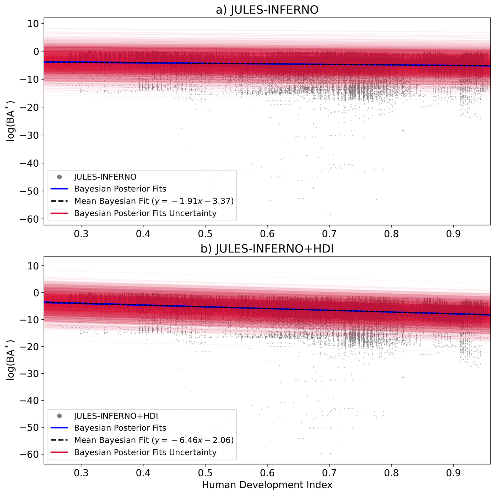
Figure 6Bayesian linear regression performed in log-space on log (BA*) with HDI as predictor for (a) JULES-INFERNO and (b) JULES-INFERNO+HDI. The grey dots represent the scatter plot of all monthly burnt area values at all grid cells as a function of HDI in the log-space. The blue solid lines represent posterior predictive samples of the fitted regression. The black dashed line represents the posterior mean fit. The red lines indicate the uncertainty envelope derived from the posterior predictive distribution. The regression results are shown in log-space.
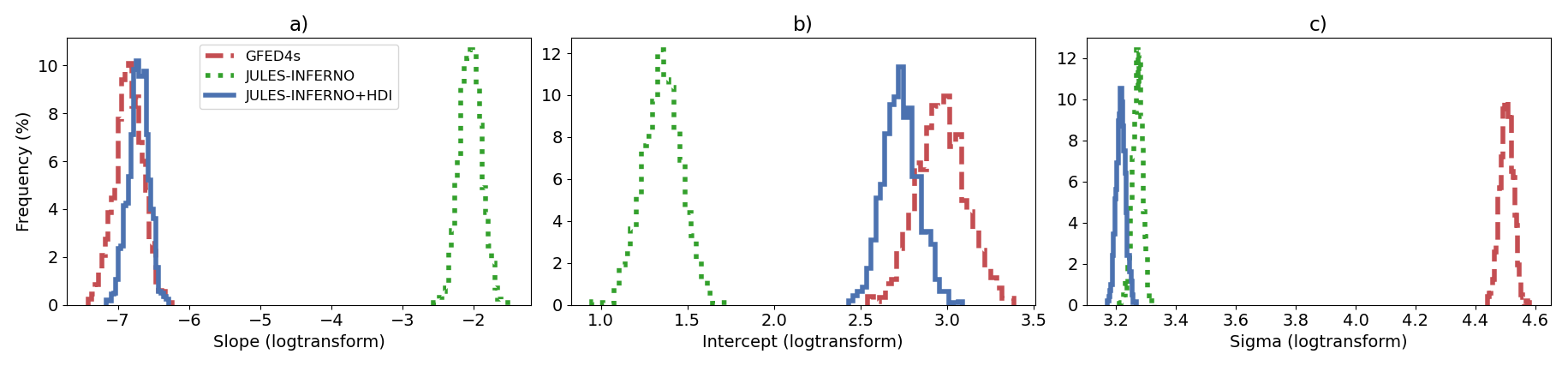
Figure 7Histograms of posterior distributions for Bayesian linear regression fit parameters derived for GFED4s (dashed red line), JULES-INFERNO (dotted green line), and JULES-INFERNO+HDI (solid blue line). Panel (a) shows the slope parameter, panel (b) the intercept parameter, and panel (c) depicts the sigma (error term representing random sampling noise) in log-transformed space.
As expected, JULES-INFERNO (the original version of the model not including the HDI) does not present a strong relationship between the FWI-trend adjusted burnt area fraction and HDI. The mean Bayesian fit slope is −1.91, indicating a weaker relationship between the variables than in JULES-INFERNO+HDI when compared to observations. In contrast, the stronger negative slope of −6.42 found in observations suggests a more pronounced socio-economic influence on fire suppression in the observational data. When HDI is explicitly incorporated to represent socio-economic effects on fire in JULES-INFERNO+HDI, the model better reproduces the relationship observed in GFED4s, with a Bayesian fit slope of −6.46. This result demonstrates an improved representation of the socio-economic impact on fire dynamics, aligning the model more closely with observations in terms of global mean dependence on HDI.
3.2 Evaluation of impact on burnt area
To better understand the regional impact of implementing the socio-economic factors on fire ignition and suppression in INFERNO, we focus on the burnt area results averaged over the GFED4s regions as defined in Fig. A1.
Both model experiments reproduce the overall geographical pattern of the annual average burnt area fraction (Fig. 8), though with some regional differences compared to observations. For instance, JULES-INFERNO simulates the observed pattern in the major fire regions: South America, Africa and Eurasia. The 2-D cross-correlation was used to determine what is referred to as spatial correlation between the model experiments and the observation data. JULES-INFERNO shows substantial spatial biases over North America, Europe and Asia, leading to a low global spatial correlation of 0.265 compared with GFED4s. Conversely, JULES-INFERNO+HDI reduces fires in the regions with higher HDI values, reducing the biases seen in JULES-INFERNO and resulting in a better agreement with GFED4s. JULES-INFERNO+HDI has a global spatial correlation of 0.465 when compared with GFED4s. However, due to the nature of the HDI data, sharp boundaries between countries can appear in the burnt area results (e.g., between Canada and the United States of America) – Fig. 1e).
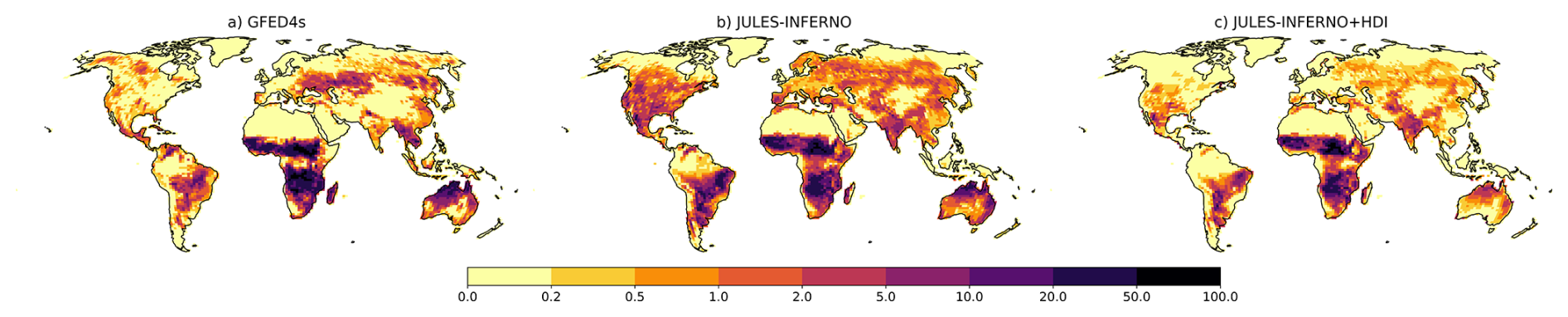
Figure 8Burnt area fraction (%) mean annual average (1997–2016) for (a) GFED4s, (b) JULES-INFERNO and (c) JULES-INFERNO+HDI. Please note that the colour mapping uses a colour axis in which the difference in colours do not correspond linearly to differences in burnt area fraction.
Representing the socio-economic factors through HDI in the parametrisation for fire ignition and suppression has an impact in all regions. However, it mostly reduces the burnt area in regions with high prosperity (high values of HDI), leading to reduced bias over North America, Europe and Asia, as shown in Fig. 9. Moreover, compared to JULES-INFERNO, JULES-INFERNO+HDI reduces the positive bias over South America and India, although it increases the negative bias over the boreal regions, Australia, and South East Asia.
To further evaluate the impact of incorporating socio-economic factors on fire dynamics in INFERNO via HDI, we present histograms depicting the frequency distribution of burnt area across different fire regions in Fig. 10. These histograms provide valuable insights into how the inclusion of socio-economic factors in JULES-INFERNO+HDI influences the occurrence of fires of different magnitudes compared to both JULES-INFERNO and GFED4s observations. To provide a quantitative assessment of model performance, the Wasserstein distance (Ramdas et al., 2017) is used as a metric of the fit between the probability distributions of the JULES-INFERNO and JULES-INFERNO+HDI histograms and the GFED4s observations. In this context, smaller values indicate better agreement between modelled and observed distributions, with a value of zero representing a perfect match and progressively larger values reflecting increasing divergence. This analysis helps to identify the dominant fire sizes in each region, assess whether the introduction of socio-economic factors leads to shifts in these distributions, and determine whether the implementation in JULES-INFERNO+HDI leads to a better representation of the burnt area probability distribution.
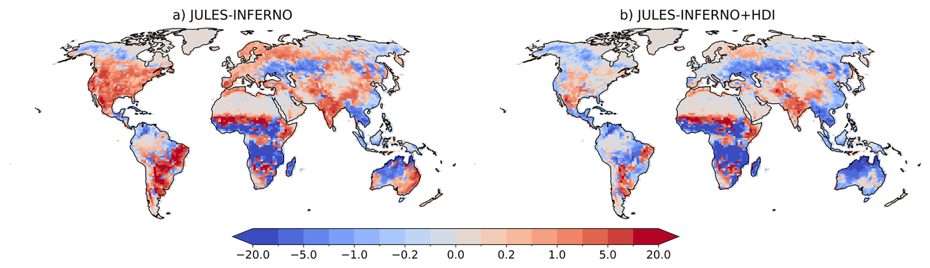
Figure 9Burnt area fraction (%) mean annual average bias (1997–2016) for (a) JULES-INFERNO, and (b) JULES-INFERNO+HDI, calculated relative to the GFED4s observations. Please note that the colour mapping uses a colour axis in which the difference in colours do not correspond linearly to differences in burnt area bias.
Globally, GFED4s observations display a steep decline in burnt area frequency as fire sizes increase, with small burnt area fractions dominating the distribution (Fig. 10a). JULES-INFERNO reproduces this dominance of small fires relatively well but exhibits a strong underestimation of the frequency of large burnt area fractions (>0.5). The introduction of HDI in JULES-INFERNO+HDI increases the frequency of the largest burnt area fractions (0.7–1.0), improving the representation of larger fire sizes relative to JULES-INFERNO. However, this improvement comes at the expense of degraded performance for small to moderate burnt area fractions (<0.5), which account for the majority of fire occurrences. This trade-off is reflected in the Wasserstein distance, which increases slightly from 0.89 % for JULES-INFERNO to 1.08 % for JULES-INFERNO+HDI at the global scale, indicating that despite the improved fit for extreme fires, this does not compensate for the deterioration across more frequent smaller fires.
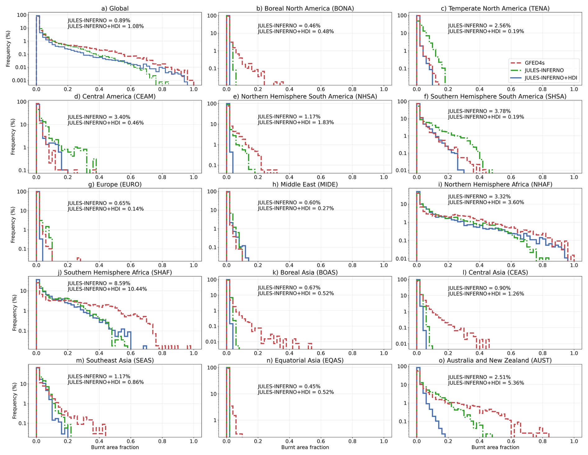
Figure 10Histograms showing the distribution of burnt area fractions across fire regions for GFED4s observations (red dashed lines), JULES-INFERNO (green dotted lines), and JULES-INFERNO+HDI (blue solid lines), for the different fire regions. Annotated values indicate the Wasserstein distance of each model experiment relative to GFED4s.
In boreal regions (Boreal North America, BONA, and Boreal Asia, BOAS), GFED4s distributions are strongly skewed towards small burnt areas, with a rapid decline in frequency beyond 0.1. Both JULES-INFERNO and JULES-INFERNO+HDI substantially under-represent moderate size fires in these regions (burnt area fractions between 0.1 and 0.4), indicating persistent challenges in capturing boreal fire dynamics. The inclusion of HDI leads to a modest additional suppression of burnt areas, but the resulting Wasserstein distances remain very similar between the two model configurations (0.46 % for JULES-INFERNO and 0.48 % for JULES-INFERNO+HDI in BONA and 0.67 % for JULES-INFERNO and 0.52 % for JULES-INFERNO+HDI in BOAS). This indicates that incorporating socio-economic factors does not provide a clear improvement or degradation in the overall agreement with observations in boreal regions, suggesting that other processes, such as fuel availability, fire weather, or ignition sources, are likely more influential in governing boreal fire regimes.
In temperate regions, including Temperate North America (TENA) and Europe (EURO), GFED4s observations again show a strong dominance of small fires (burnt area fractions <0.1). In TENA, JULES-INFERNO markedly overestimates burnt area fractions greater than 0.1, while JULES-INFERNO+HDI substantially reduces this bias. This improvement is quantitatively supported by a pronounced reduction in Wasserstein distance from 2.56 % to 0.19 %, indicating a clear overall improvement across the full distribution. For EURO, although JULES-INFERNO+HDI reduces the occurrence of larger fires, it also underestimates small and moderate burnt area fractions. Consequently, the Wasserstein distance decreases from 0.65 % in JULES-INFERNO to 0.14 % in JULES-INFERNO+HDI, suggesting a closer overall distributional match, but Fig. 10g shows that this improvement does not consistently reflect better performance across all fire size classes. In particular, JULES-INFERNO better captures the frequency of small fires, which dominate the observed distribution, indicating that the apparent improvement in the Wasserstein distance should be interpreted cautiously.
In Central America (CEAM) and Southern Hemisphere South America (SHSA), GFED4s exhibits broader distributions with contributions from small to moderate burnt areas. JULES-INFERNO strongly overestimates moderate and large fires in both regions, leading to large Wasserstein distances (3.40 % and 3.78 %, respectively). The inclusion of HDI substantially narrows the distributions and reduces the occurrence of large fires, resulting in marked reductions in Wasserstein distance (to 0.46 % in CEAM and 0.19 % in SHSA). These results indicate a genuine improvement across most of the distribution, including the dominant fire sizes. In African savanna regions (Northern Hemisphere Africa, NHAF, and Southern Hemisphere Africa, SHAF), GFED4s shows relatively high frequencies of large burnt areas. Both experiments underestimate extreme fire sizes, but JULES-INFERNO+HDI increases the suppression of medium fires further, leading to mixed results. In NHAF, the Wasserstein distance increases from 3.32 % in JULES-INFERNO to 3.60 % in JULES-INFERNO+HDI, while in SHAF it increases from 8.59 % to 10.44 %, indicating a degradation in overall distributional agreement despite improvements in larger fire sizes.
Across Asian regions (EQAS, CEAS, SEAS) and Australia and New Zealand (AUST), GFED4s distributions are dominated by small to moderate burnt area fractions. Both experiments under-predict medium-sized burnt area fractions (e.g., 0.2–0.6), with JULES-INFERNO+HDI generally exacerbating this negative bias. This is reflected in increased Wasserstein distances for JULES-INFERNO+HDI in CEAS (0.90 % for JULES-INFERNO and 1.26 % for JULES-INFERNO+HDI) and AUST (2.51 % for JULES-INFERNO and 5.36 % for JULES-INFERNO+HDI), indicating that the additional HDI-related reduction in fire activity (through both ignition and suppression processes) reduces agreement with observations across the most frequent fire sizes.
Overall, the introduction of a socio-economic representation of fire suppression in JULES-INFERNO+HDI reduces the frequency of large burnt areas and corrects strong positive biases present in JULES-INFERNO in several regions, notably TENA, CEAM, and SHSA. However, these improvements are often accompanied by a deterioration in the representation of small and moderate burnt area fractions, which dominate fire occurrence globally. As reflected by the Wasserstein distance, JULES-INFERNO+HDI does not consistently outperform JULES-INFERNO across all regions, particularly in savanna-dominated regions such as Africa, Australia, and parts of Eurasia. These results highlight the need for further refinement of the socio-economic parametrisation and the inclusion of additional region-specific processes to improve the simulation of fire size distributions across all fire regimes.
Figure 11 shows the burnt area annual mean time series. To assess the ability of the model to reproduce the observed time series, we perform a statistical analysis based on monthly averaged data, including the calculation of various metrics such as the Root Mean Squared Error (RMSE), Root Mean Squared Error after removal of a constant mean bias (RMSEUB), the bias, Pearson correlation, and the Standard Deviation (SD) of the burnt area monthly and annual mean time series for all GFED4s regions (Table A1). The SD is computed after removal of a linear trend. We also assess the model's ability to reproduce observed trends using a simple log-transformed linear regression. Figure 12 summarises these statistical measures for both model configurations.
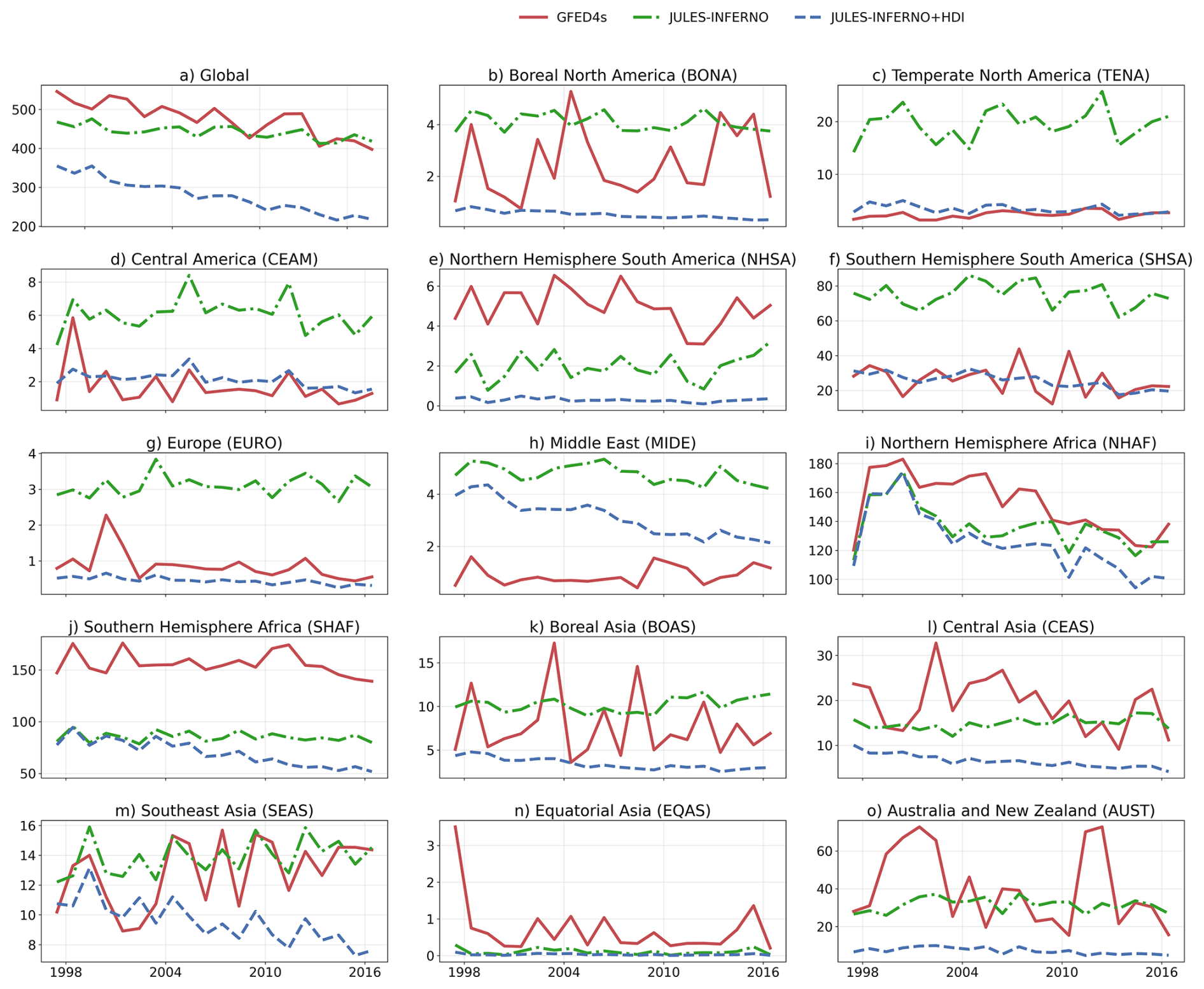
Figure 11Time series of annual mean burned area (Mha) from 1997 to 2016 across different fire regions, shown for GFED4s (solid red line), JULES-INFERNO (green dot-dash line), and JULES-INFERNO+HDI (blue dashed line).
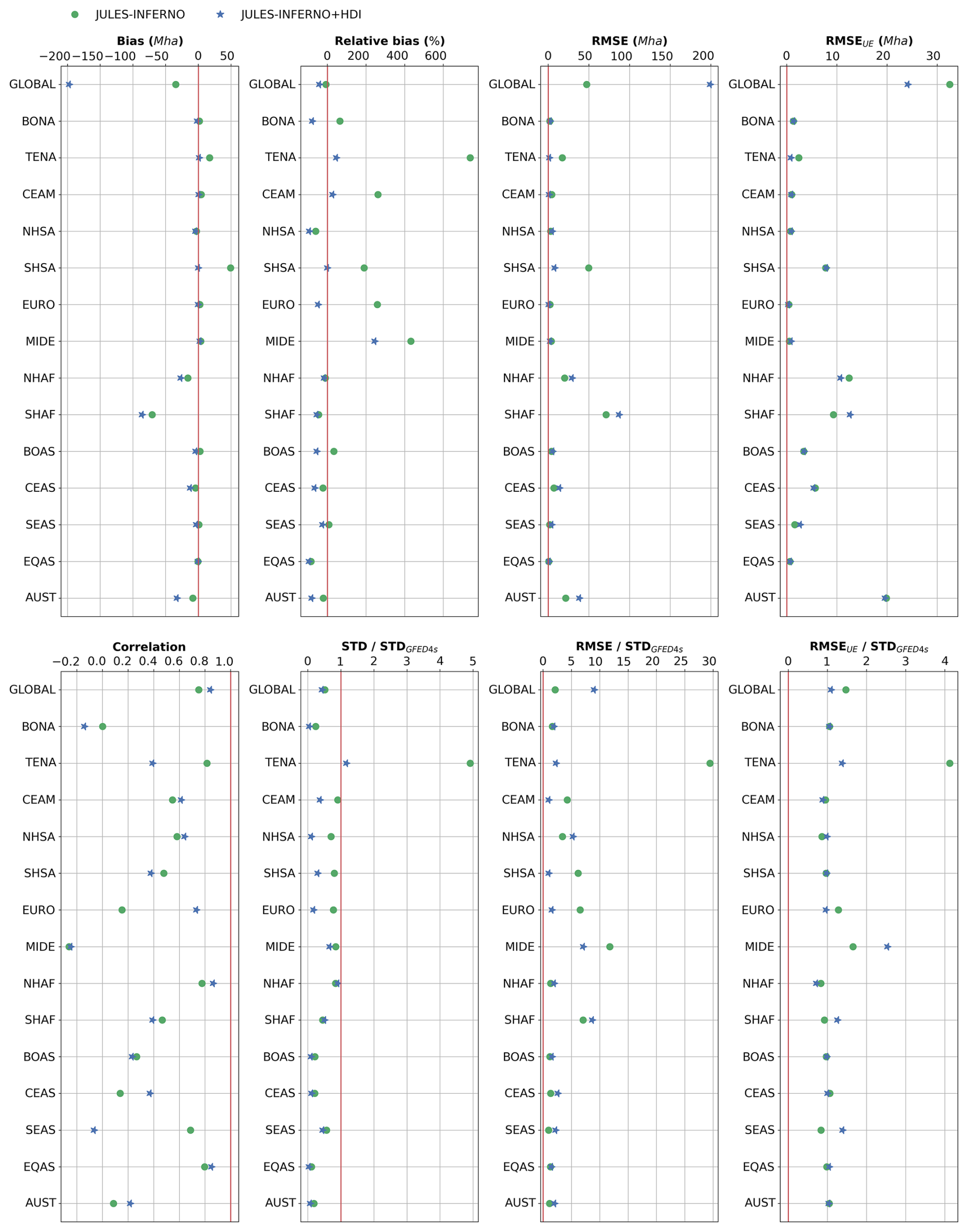
Figure 12Summary of the statistics presented in Table A1 comparing JULES-INFERNO (green circle) and JULES-INFERNO+HDI (blue star). The red line show the reference value for a perfect simulation, the closer the experiment symbol is from this line the better.
The results presented in Figs. 11 and 12, together with the regional statistics in Table A1, show that the inclusion of socio-economic factors in INFERNO leads to regional improvements in the simulation of burnt area in regions where JULES-INFERNO bias exhibits the largest deviations from GFED4s (greater than 150 %). For example, the relative bias in TENA is reduced from 735.6 % in JULES-INFERNO to 44.5 % in JULES-INFERNO+HDI, in CEAM from 259.2 % to 24.2 %, in SHSA from 191.7 % to −1.7 %, in EURO from 258.8 % to −48.8 %, and in MIDE from 420.5 % to 231.8 % (Table A1). These reductions are also accompanied by decreases in RMSE, indicating an improved agreement between JULES-INFERNO+HDI and GFED4s for these regions.
Conversely, some regions experience a smaller, but still notable, increase in relative bias. For example, relative bias in Northern Hemisphere South America (NHSA) changes from −60.1 % to −94.3 %, in Australia (AUST) from −21.8 % to −82.3 %, and in Southern Hemisphere Africa (SHAF) from −45.3 % to −55.3 %. This highlights that the inclusion of HDI does not uniformly improve model performance in all regions, reflecting a trade-off between correcting large positive biases and potentially amplifying negative biases in other areas.
In addition, the inclusion of HDI is associated with a systematic reduction in the simulated variability. The ratio of modeled to observed standard deviation (SD SDGFED4s), calculated from detrended monthly mean values, decreases in most regions. For instance, SD SDGFED4s decreases from 4.41 to 1.04 in TENA, from 0.25 to 0.11 in BONA, from 0.84 to 0.34 in CEAM, from 0.77 to 0.28 in SHSA, and from 0.68 to 0.15 in SHSA, indicating an underestimation of sub-annual variability. While this reduction in variability can contribute to lower RMSE in some regions, it also suggests that in JULES-INFERNO+HDI the amplitude of burnt area fluctuations is damped relative to observations.
At the global scale, JULES-INFERNO exhibits a relatively small mean bias due to compensating regional errors. The inclusion of HDI reduces these compensating effects, resulting in a larger negative global relative bias (from −7.21 % in JULES-INFERNO to −41.46 % in JULES-INFERNO+HDI) and an increase in RMSE (from 42.28 to 198.99). Nevertheless, RMSEUB decreases from 32.50 to 24.12, and the Pearson correlation with GFED4s increases from 0.75 to 0.84, reflecting an improved representation of temporal co-variability of monthly burnt area.
Overall, the inclusion of socio-economic factors in INFERNO through HDI results in a trade-off. JULES-INFERNO+HDI improves the mean-state representation in regions with the largest bias in JULES-INFERNO (TENA, CEAM, SHSA, EURO, MIDE). However, relative biases worsen in regions where burnt area is underestimated in JULES-INFERNO (NHSA, SHAF, AUST), and variability is generally reduced.
Nonetheless, the improvements from JULES-INFERNO+HDI in regions such as TENA, NHAF, and SHAF have a greater impact on the global metrics than the reduced performance seen for regions such as CEAM, NHSA, SHSA, EURO, and MIDE. For regions such as BOAS, CEADS, SEAS, EQAS, and AUST, both model configurations underperform in terms of standard deviation, and any relative difference in SD SDGFED4s between both are small when compared to the observed standard deviation (e.g., difference between the JULES-INFERNO and JULES-INFERNO+HDI SD SDGFED4s smaller than 15 %).
Furthermore, for some of these regions INFERNO is not expected to agree well with observations, especially in terms of variability, as the fire behaviour of some of these regions is characterised by mechanisms that are not represented in INFERNO. This will be further discussed in Sect. 4.
3.3 Impact on burnt area trends
Representing the socio-economic factors through HDI in INFERNO adds a new external constraint to the model. Through this, historical changes to socio-economic factors influence how changes in population density affect fire ignitions in the model (see Sect. 2.3 and Fig. 4). Specifically, for regions with high HDI, variations in population have less of an impact on anthropogenic ignitions, while for regions with low HDI, variations in population can have a more considerable impact. This alters the importance of population density changes for highly developed regions, making HDI the dominant factor shaping burnt area trends.
As shown in Fig. 13, both JULES-INFERNO and JULES-INFERNO+HDI represent the main global burnt area trends. JULES-INFERNO is able to represent the regions with burnt area increases (e.g., Southern Africa and Northeast South America) and captures the dominant region for decreased burnt area – North Africa. However, this model setup tends to have weaker negative trends when compared to GFED4s. Conversely, JULES-INFERNO+HDI presents stronger trends, better representing those found in observations. However, it does not reproduce the positive trends in Southern Africa and Northeast South America. Both JULES-INFERNO and JULES-INFERNO+HDI are unable to represent the observed trends in Central Asia or Boreal North America.
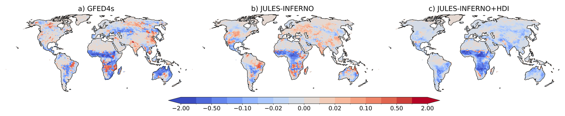
Figure 13Burnt area fraction trend (% yr−1) (calculated between the period 1997–2016) for (a) GFED4s, (b) JULES-INFERNO and (c) JULES-INFERNO+HDI. Please note that the colour mapping uses a colour axis in which the difference in colours do not correspond linearly to differences in burnt area fraction trend.
Nonetheless, it should be noted that over the 2001–2012 period, Andela and Van Der Werf (2014) estimated that 51 % of the upward trend over southern Africa can be attributed to El Niño-Southern Oscillation (ENSO), while there is also evidence that socio-economic developments can be responsible for a decline. The relation between ENSO and annual burned area depends both on the effect of ENSO on precipitation and on the antecedent precipitation-burned area response. While the model setup is able to capture ENSO variability, as its weather is driven by reanalysis, there is no mechanism that allows INFERNO to represent the antecedent precipitation-burned area effects due to litter build up. This is a limitation of the model and it should not be expected for the model to perform well in regions where this precipitation-burned area coupling can be dominant, such as Central America, Northern Hemisphere South America, Europe, Northern Hemisphere Africa, and Central Asia (Andela et al., 2017; Abatzoglou et al., 2018).
Overall, representing the socio-economic factors through HDI in INFERNO results in an improvement in burnt area trends in comparison with observations. As seen in Table A1, JULES-INFERNO+HDI better represents the global negative trend in burnt area when compared to observations (−6.77 Mha yr−1 for GFED4s, −2.24 Mha yr−1 for JULES-INFERNO, and −7.58 Mha yr−1 for JULES-INFERNO+HDI). This improvement comes mostly from a better representation of the burnt area trends in regions with strong negative trends, such as SHSA, NHAF, CEAS and AUST, but also by better representing regions with weak negative burnt area trends, namely CEAM, NHSA, EURO and BOAS. Moreover, in regions such as CEAM, NHSA, EURO, BOAS, CEAS, and AUST, JULES-INFERNO+HDI shows a negative burnt area trend, in better agreement with observations.
Contrary to these improvements, JULES-INFERNO+HDI can also produce trends that are too strong, reflecting the presence of compensating biases in the model. For example, in Southern Hemisphere Africa (SHAF), although JULES-INFERNO+HDI reproduces the observed negative burnt area trend, the magnitude of the trend is substantially overestimated (−0.54 Mha yr−1 for GFED4s, −0.14 Mha yr−1 for JULES-INFERNO, and −1.94 Mha yr−1 for JULES-INFERNO+HDI). In this region, the improved agreement in the sign of the trend in JULES-INFERNO+HDI arises from compensating biases that mask an excessive sensitivity to human influence, whereas JULES-INFERNO provides a more realistic representation of the trend magnitude. This example highlights that, as for JULES-INFERNO, apparent improvements in some metrics in JULES-INFERNO+HDI, such as regional or global trends, can result from compensating errors rather than an overall improvement in process representation.
Nonetheless, the observed dataset (GFED4s) shows that out of 14 regions, four have positive burnt area trends (Table A1). JULES-INFERNO only presents a positive trend for TENA and SEAS. While JULES-INFERNO+HDI tends to enforce decreasing trends, this only happens in four regions out of 14 (i.e., TENA, SHAF, MIDE, and SEAS). For the remaining 10 regions, JULES-INFERNO+HDI presents a similar trend to JULES-INFERNO or even an improved trend when compared to GFED4s.
It should be noted that limitations of the INFERNO fire model, including its representation of fire behaviour and the processes governing large and severe fires, are discussed in detail in the Discussion Sect. 4.2. These limitations should be considered when interpreting regional biases and model performance across different fire regimes.
3.3.1 Impact of external model drivers on burnt area trends
As described in Sect. 2.4, the JULES-ES experimental setup relies on ancillary forcing data to represent external processes to JULES, such as atmospheric weather conditions, atmospheric composition, population density, and biogenic drivers. These external forcings can drive fire by forcing changes to the evolution of land surface properties, fire ignitions, and fire weather. It is important to understand the impact these external drivers have on the burnt area trends and the interaction with the parametrised socio-economic factors in fires. Therefore a set of sensitivity experiments was performed by fixing the external model drivers to the year 1990 and only allowing an individual external driver to vary transiently through the experiment.
-
1990 control: where all external model drivers are fixed to year-1990 values
-
clim: where only the atmospheric drivers are transient (downward longwave radiative flux, downward shortwave radiative flux, precipitation, surface pressure, air temperature, meridional and zonal wind components)
-
tas: where only air temperature at 2 m is transient
-
ppn: where only precipitation is transient
-
lu: where only the land use is transient
-
Ndep: where only Nitrogen deposition is transient
-
pop: where only population density is transient
-
CO2: where only the atmospheric carbon dioxide (CO2) mixing ratio is transient
-
HDI: where only the Human Development Index is transient (only for JULES-INFERNO+HDI)
These sensitivity experiments branched from their respective control runs – JULES-INFERNO and JULES-INFERNO+HDI – starting from 1990 and run up to 2016. In this way, the underlying land surface state from the reference run is preserved, and only changes to the forcing that take place during the period of interest are taken into effect. The trends for each relevant external forcing are in Supplementary Fig. A2.
The results of these sensitivity experiments on the burnt area trends (Mha yr−1), and respective standard error, for the different GFED4s fire regions are presented in Table A2 in the Appendix for JULES-INFERNO and Table A3 for JULES-INFERNO+HDI. These results are summarised in Fig. 14. Burnt area trends in JULES-INFERNO tend to be driven by climate, land use, or population density changes (relative contribution greater than 50 % when compared to control), with the dominant driver (the sensitivity experiment with the largest absolute trend value) for the majority of regions being climate (including through air temperature and precipitation), for example, BONA, TENA, NHSA, SHSA, EURO, MIDE, SHAF, BOAS, CEAS, SEAS, and AUST. On the one hand, air temperature is a dominant, and statistically significant, driver of increasing burnt area trends for CEAM, NHSA, BOAS and CEAS. For MIDE, precipitation has a dominant role in reducing burnt area. On the other hand, despite dominating the burnt area trends, temperature can have opposite effects on the sign of the trend. Namely, for TENA, SHSA, EURO, and AUST, where temperature results in an increase in the trend.
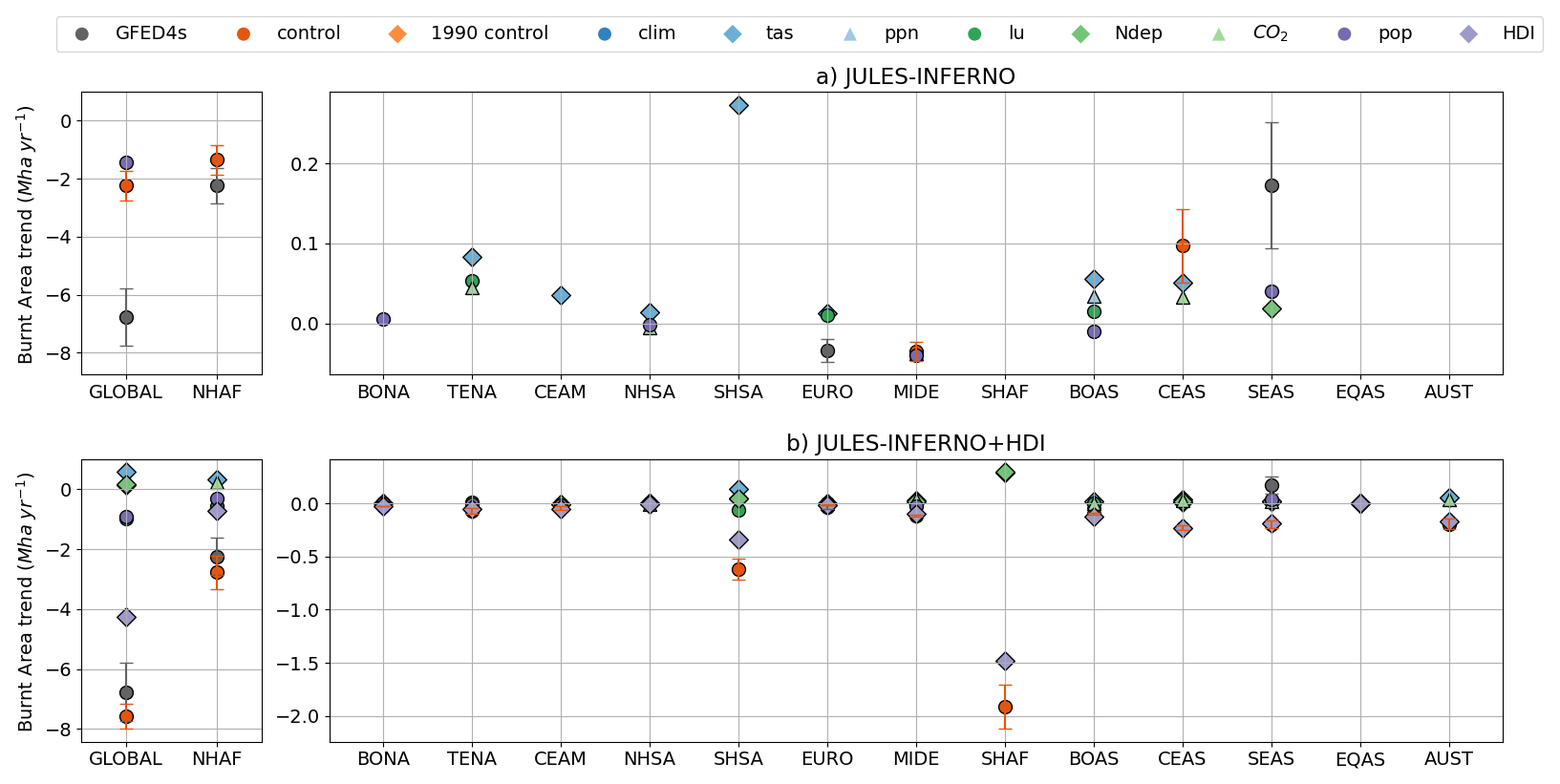
Figure 14Burnt area trends (Mha yr−1) for the different GFED4s fire regions (Giglio et al., 2013) from the model sensitivity experiments for (a) JULES-INFERNO and (b) JULES-INFERNO+HDI. Only trends that are statistically significant at the 95 % confidence level are shown. The whiskers for the values of GFED4s and control represent the standard error associated with the trend. GLOBAL and NHAF regions are presented in separate panels to improve readability, due to their large trends compared to other regions. Only the GFED4s and control datasets include whiskers representing the standard error of the estimated trends; uncertainty ranges for the remaining sensitivity experiments are not shown to maintain clarity in an already complex figure.
Anthropogenic drivers, such as land use and population density can play a major role in some regions. For example, land use is the dominant driver in SHSA and SHAF, population density in CEAM, and both are important drivers in TENA, EURO, MIDE, NHAF. Land use can cause either an increase (TENA, EURO, and SHAF) or a decrease in burnt area, while population density results in a reduction in burnt area for all the regions where this external driver is dominant (TENA, CEAM, EURO, MIDE, and NHAF).
Biogenic drivers such as nitrogen deposition and atmospheric carbon dioxide assimilation generally play a more limited role in burnt area trends compared to climate and land-use drivers, but they can still be important in specific regions and for aggregated global trends. Nitrogen deposition is a significant driver of global burnt area trends in JULES-INFERNO+HDI, while atmospheric carbon dioxide assimilation impacts trends in NHSA, and both nitrogen deposition and atmospheric carbon dioxide influence CEAS.
For JULES-INFERNO+HDI, HDI is the dominant factor in the burnt area trend for all regions, with the exception of NHAF and EQAS. This is evident in the sensitivity experiments for JULES-INFERNO+HDI where only HDI forcing is made transient (HDI). In all cases, representing the socio-economic factors through HDI in INFERNO changes the relative role that external forcings have in determining burnt area trends. For example, it reduces the role that climate, population density, and land use have in burnt area trends towards a stronger role from socio-economic effects (HDI).
This impact is especially evident when comparing the role of the climate forcing in driving burnt area trends between JULES-INFERNO and JULES-INFERNO+HDI in their respective sensitivity experiments, clim, tas, and ppn. For instance, for regions where temperature effects on burnt area trends were dominant in JULES-INFERNO, they show less of an impact from temperature in JULES-INFERNO+HDI, albeit still at a statistically significant level (e.g., TENA, EURO, CEAS, and AUST). In addition, where the climate contributions to the burnt area trends were small in JULES-INFERNO (BONA, CEAM, and NHSA), when considering socio-economic factors, these become statistically non-significant in terms of the climate contributions to the trends. In addition, representing socio-economic factors through HDI in INFERNO leads to changes in how precipitation and temperature influence burnt area trends in some regions. For example, in MIDE, precipitation contributes to a negative burnt area trend in JULES-INFERNO (−0.038 Mha yr−1). In JULES-INFERNO+HDI, the contribution from precipitation is reduced (−0.016 Mha yr−1), while temperature shows an increased positive contribution to the burnt area trend (+0.034 Mha yr−1). A similar pattern is also seen for NHAF, where the role of temperature becomes statistically significant in JULES-INFERNO+HDI (+0.342 Mha yr−1).
Moreover, results show a difference in the role of anthropogenic drivers (land use and population density) on burnt area trends between JULES-INFERNO and JULES-INFERNO+HDI sensitivity experiments. For BONA, CEAM, and NHSA regions, burnt area decreases for JULES-INFERNO+HDI (pop and lu) sensitivity experiments while for JULES-INFERNO (pop and lu) an increase was simulated.
Together, these results indicate that representing socio-economic factors through HDI can influence the simulation of burnt area in ESMs, but that its impact is regionally heterogeneous and involves clear trade-offs. The inclusion of HDI in JULES-INFERNO primarily improves the mean-state representation and trend magnitude in regions where the original model exhibits strong positive biases. However, these improvements are not uniform across all fire regions. In several regions the additional constraint imposed by the use of HDI as a proxy for socio-economic impacts on fire leads to reduced variability or amplified negative biases. Overall, JULES-INFERNO+HDI demonstrates that socio-economic development can be an important modulator of fire activity and trends at regional scales, but further refinement of JULES-INFERNO+HDI is still required to better balance its effects across different fire regions.
Results from this work indicate that incorporating socio-economic factors via HDI in the fire ignition and suppression parametrisation within INFERNO, alongside revised parameters, improves the globally-averaged relationship between burnt area and HDI (Figs. 3 and 6). This reduces large positive biases previously seen in JULES-INFERNO. However, improvements are regionally variable, and in some areas the inclusion of HDI introduces trade-offs, such as reduced variability or poorer representation of small to moderate fires, highlighting the need for further refinement.
The HDI representation captures the general tendency for socio-economic processes to suppress fires with increasing development. We assume a linear relationship between burnt area and HDI for simplicity, but this does not imply the observed relationship is linear. The result should be interpreted as conditional on the model form, representing a statistical approximation rather than a physical linear relationship.
This approach suggests that regions with higher HDI tend to have lower average values of burnt area. This trend can be attributed to various components of HDI that influence government policies and resources for fire management (Miranda-Lescano et al., 2023). Income reflects economic capacity for wildfire management. For example, Rideout et al. (2017) show how budgeting tools like STARFire support allocation of resources across suppression and fuel treatments. Health impacts from wildfire smoke also motivate mitigation and adaptation responses (Rizzo and Rizzo, 2024), including early warning and risk communication. Education may also reduce ignitions through awareness and preparedness. For example, wildfire prevention education in Florida was associated with fewer human-caused ignitions across several categories (Prestemon et al., 2010). Collectively, these factors support HDI as a proxy for socio-economic influences on fire management, though it cannot capture regional specifics.
Large bias reductions occur in TENA, CEAM, SHSA, EURO, and MIDE. However, performance degrades in AUST and SEAS, where negative biases increase. JULES-INFERNO shows strong positive regional biases (>150 %), which compensate for negative biases and reduce the global bias. Removing this compensation leads to a larger negative global bias in JULES-INFERNO+HDI. This highlights the importance of regional evaluation, as good global performance partly results from compensating regional errors.
The histograms of burnt area frequency across different fire regions (Fig. 10) show key differences in how fire sizes are distributed between JULES-INFERNO, JULES-INFERNO+HDI, and GFED4s. JULES-INFERNO+HDI improves the frequency distribution in TENA, CEAM, and SHSA by reducing overestimated large fires. In NHAF, JULES-INFERNO+HDI further suppresses medium to large fires but does not consistently improve agreement with GFED4s. In NHSA and AUST, the underprediction of medium and large fires worsens, highlighting regional trade-offs. JULES-INFERNO+HDI also improves burnt area trends, particularly where these are negative in GFED4s. JULES-INFERNO often shows no significant trends (e.g., SHSA, NHAF, CEAS, AUST) and better represents weak negative trends (CEAM, NHSA, EURO, BOAS). However, JULES-INFERNO+HDI can produce overly strong negative trends (e.g., SHAF) or misrepresent positive trends in TENA, MIDE, BONA, and SEAS.
Overall, JULES-INFERNO+HDI improves representation of burnt area trends compared to JULES-INFERNO, highlighting the importance of socio-economic factors in ignition and suppression. This is particularly evident in sensitivity experiments, where including socio-economic impacts reduces the role of climate drivers in burnt area trends, especially temperature and precipitation, with socio-economic drivers becoming dominant.
4.1 Model sensitivity to external drivers
We have shown that introducing socio-economic factors alters the contribution of external drivers to burnt area trends, with clear regional variability. The inclusion of these factors reduces or modifies the role of temperature in driving trends (e.g. TENA, EURO, CEAS, and AUST), while also changing the influence of climate drivers more generally in regions such as MIDE, NHAF, and SEAS. In addition, socio-economic factors increase the influence of land use and population density on fire activity by changing how human activity interacts with fire regimes (e.g. BONA, CEAM, and NHSA).
Although HDI does not explicitly encompass the impacts of fire management policies, these results are consistent with previous studies demonstrating that, in highly developed regions, institutional capacity and land-management policies exert a stronger control on fire activity than individual ignition behaviours.
The results from Sect. 3.3.1 show that anthropogenic drivers (land use, population density, and HDI), together with precipitation, dominate the global burnt area trend. This is consistent with the work of Kelley et al. (2019), Jones et al. (2022), and (Andela et al., 2017), which show that despite widespread increases in fire weather severity and fire weather season length, burnt area trends vary regionally, with significant declines mainly in Africa (NHAF and SHAF), Europe (EURO), and Central Asia (CEAS), driven in part by reduced savannah-grassland burning from agricultural expansion and changes in vegetation productivity linked to hydrological shifts.
The inclusion of anthropogenic drivers (land use and population density) leads to reduced burnt area trends in JULES-INFERNO+HDI compared to JULES-INFERNO in regions such as BONA, CEAM, and NHSA. Combined with a reduced sensitivity to temperature, this improves performance in parts of South America (NHSA and SHSA). This behaviour is consistent with observations from regions such as the Mediterranean, where declines in burnt area have occurred despite increasing fire weather severity and are attributed to improved suppression and fire management (Rabin et al., 2017; Jones et al., 2022). A similar mechanism is evident in Amazonia, where fire activity is closely linked to land use and deforestation (Silva Junior et al., 2021), with reductions in deforestation contributing to declines in burnt area, although modulated by drought conditions (Nepstad et al., 2014; Aragão et al., 2018).
In contrast, increases in large and severe fires have been observed in the continental United States (Goss et al., 2020; Williams et al., 2019; Abatzoglou and Williams, 2016) and boreal regions such as Canada and Alaska (Kasischke and Turetsky, 2006; Stocks et al., 2002; Veraverbeke et al., 2017), where fire activity remains strongly linked to fire weather.
4.2 Model limitations and known issues
The inclusion of socio-economic factors in INFERNO via HDI reduces inter-annual variability of burnt area across most fire regions (Fig. 11). While this improves performance in regions such as TENA and CEAM, it leads to an overall reduction in variability, limiting the model's ability to represent regions characterised by high inter-annual variability, including BONA, BOAS, AUST, CEAS, SHSA, and NHSA. Although HDI exacerbates the underestimation of variability in JULES-INFERNO+HDI, it should be noted that JULES-INFERNO also underestimates variability relative to observations despite exhibiting higher spread.
Furthermore, INFERNO is designed for Earth System Model resolutions and timescales and relies on the mean burnt area per plant functional type () formulation (Eq. 5). This approach does not resolve fine-scale fire spread processes and therefore cannot explicitly represent large and severe fire events, which likely contributes to the biases identified in regions dominated by extreme fire behaviour. Even in models with explicit fire spread schemes, these dynamics remain constrained by ESM spatial and temporal resolution. As a result, such regions may exhibit biases in burnt area and fire emissions, as well as in their simulated response to climate change.
In addition, A key limitation of JULES-INFERNO+HDI is its spatial scale, as HDI is primarily available at national level and cannot capture sub-national heterogeneity in socio-economic activity. It also does not explicitly represent regional differences in fire management practices or policy, which are important drivers of variability.
Another limitation in INFERNO is the absence of peat burning, which contributes to negative biases in equatorial Asia and boreal regions where peat fires are significant (Teixeira et al., 2021). Recent developments (Blackford et al., 2024) may improve representation and reduce these biases.
(Forkel et al., 2019) show that many global fire models fail to capture the sensitivity of burnt area to vegetation properties such as leaf area index and productivity, leading to systematic biases in fuel availability and fire behaviour. In JULES-INFERNO, Teixeira et al. (2021) identify a large (∼ 50 %) underestimation of burnt area in northern Africa (NHAF) in INFERNO, linked to an overly southward extension of bare soil into the Sahel and a resulting underrepresentation of grasslands, driven by biases in simulated precipitation and monsoon dynamics (Sellar et al., 2019b; Williams et al., 2018).
Despite improvements to vegetation-fire coupling in JULES (Burton et al., 2019), structural vegetation biases remain, including an underrepresentation of needleleaf trees in boreal regions, which affects fire regime simulation.
Finally, the large inter-annual variability observed in some regions may reflect mechanisms not fully represented in INFERNO. In regions undergoing strong anthropogenic modification, shifts in fire regimes are often driven by changes in management rather than climate alone. For example, Kirillina et al. (2020); Andela and Van Der Werf (2014) show shifts in peak fire activity linked to land use and policy changes, while prescribed burning has reduced large fires in Australia. Similarly, variability in Southern Europe, North Africa, and South America is strongly influenced by fuel continuity and socio-economic drivers (Chergui et al., 2018; Chuvieco et al., 2021).
4.3 Concluding remarks
This study demonstrates that incorporating socio-economic impacts on fire through HDI in INFERNO provides a simple and effective representation of human influences on fire activity. This improves model bias in several regions, but improvements are regionally variable, highlighting the trade-offs associated with this simplified approach.
Improvements in regions such as TENA, NHAF, and SHAF have a strong influence on global metrics, while reduced performance in CEAM, NHSA, SHSA, EURO, and MIDE partly offsets these gains. In BOAS, CEADS, SEAS, EQAS, and AUST, both configurations underperform in variability, with relatively small differences in standard deviation (generally <15 % relative to GFED4s). These results show that while HDI improves global metrics, regional performance remains heterogeneous and variability is still not well captured.
For NHSA, BOAS, CEAS, and AUST, biases increase in JULES-INFERNO+HDI. These limitations are discussed in Sect. 4.2, including missing fire processes and vegetation biases. Future improvements could include fire intensity, fuel type, seasonal timing, and vertical transport processes to better represent emissions and their atmospheric impacts.
Perkins et al. (2024) propose an alternative framework for representing human influences in INFERNO. While the WHAM! approach is more comprehensive, its complexity may limit direct application in an ESM context. In contrast, the method here is simple and directly implementable within JULES-INFERNO.
Considering this, we recommend that socio-economic factors should be included in all fire modelling studies at both global and regional scales, particularly when considering future climate change scenarios. This work will form the basis of a future study on understanding the impact of fires in the Earth System when considering future climate change scenarios.
A1 Burnt area evaluation
To analyse the model performance, we calculated the following statistical and error measures, relative to the observed (GFED4s) and modelled (JULES-INFERNO and JULES-INFERNO+HDI) burnt area:
-
Deviation of the modelled data in relation to observed values:
-
Bias, which represents the mean deviation of the modelled data in relation to the observed values.
-
The Root Mean Square Error.
-
The Root Mean Square Error after the removal of a constant bias.
-
Standard deviation for the modelled – Eq. (A5) – and observed – Eq. (A6) – data.
were i is the temporal index and N is the number of elements of ϕ considered, and is the constant bias.
Considering these statistics, a perfect simulation would have the following criteria:
-
RMSE = 0
-
RMSEUB=0
-
bias = 0
-
Pearson correlation = 100 %
-
SD SDGFED4s=1
-
RMSE SDGFED4s=0
-
RMSESDGFED4s=0
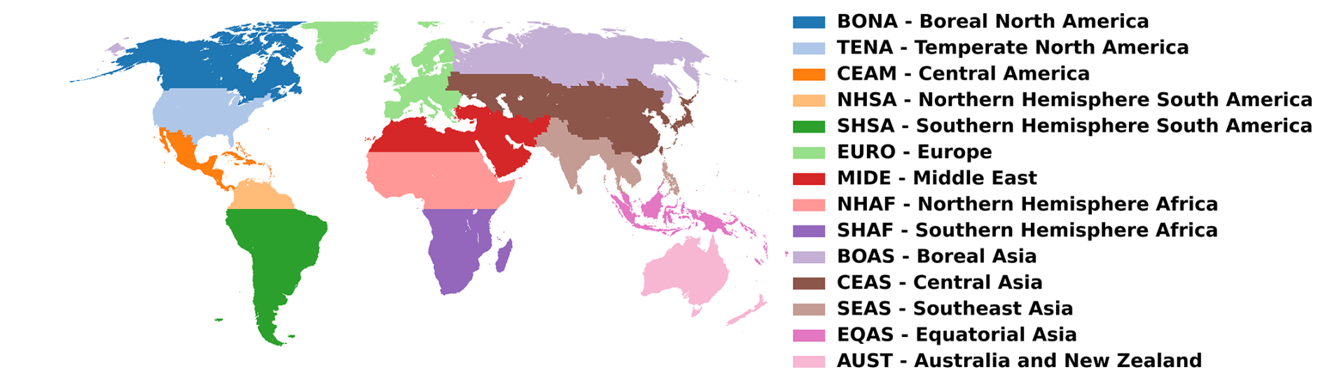
Figure A1Basis regions, as defined in the GFED4s dataset (Giglio et al., 2013).
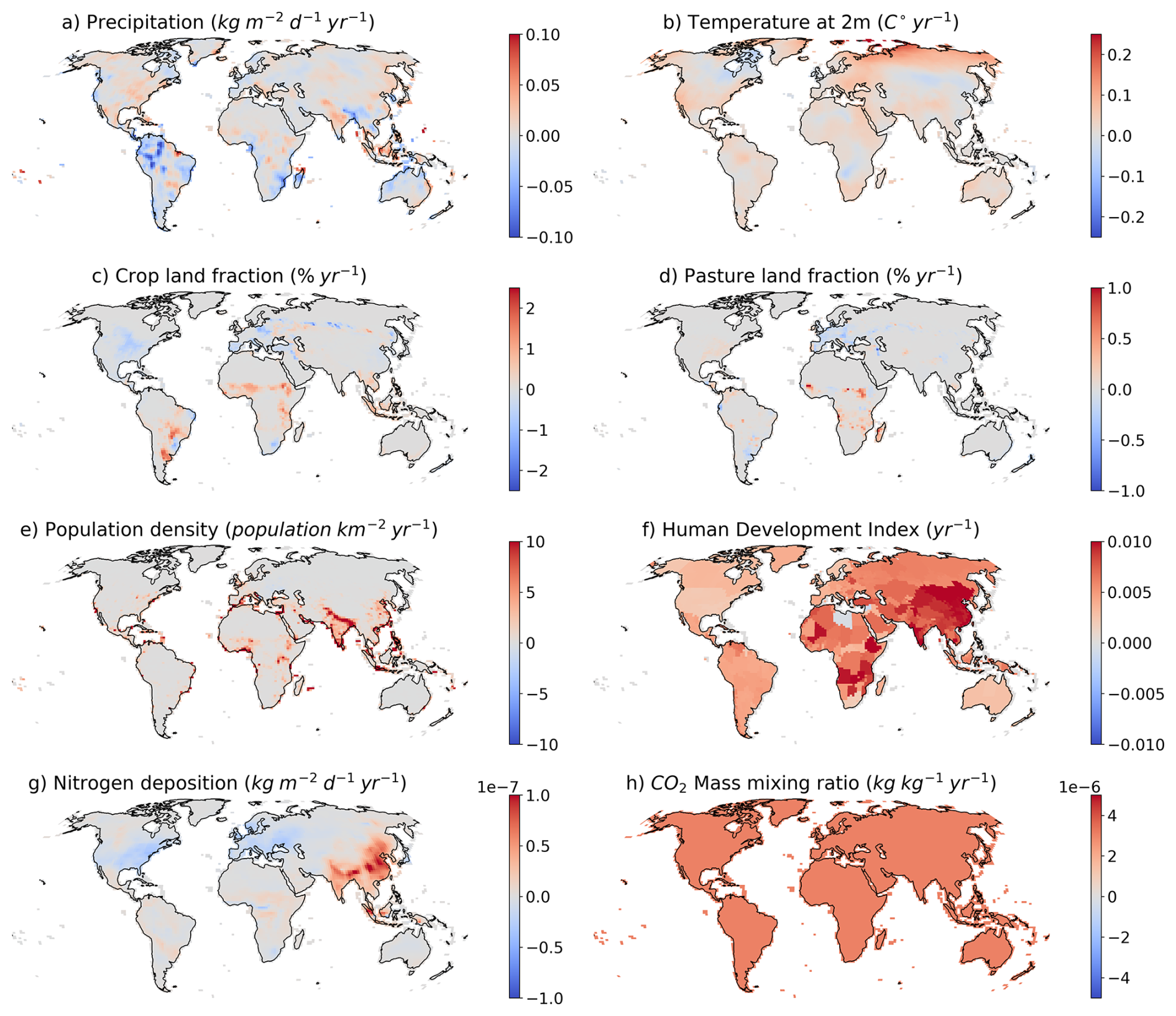
Figure A2Trends calculated between the period 1997–2016 for JULES-ES external forcing variables (a) Precipitation (kg m−2 d−1 yr−1), (b) Temperature at 2 m (C° yr−1), (c) Crop land fraction (% yr−1), (d) Pasture land fraction (% yr−1), (e) Population density (population km−2 yr−1), (f) Human Development Index (yr−1), (g) Nitrogen deposition (kg m −2 d−1 yr−1), and (h) Carbon Dioxide mixing ration (kg m−2 d −1 yr−1).
Table A1Annual burnt area statistics for the different GFED4s fire regions (Giglio et al., 2013).
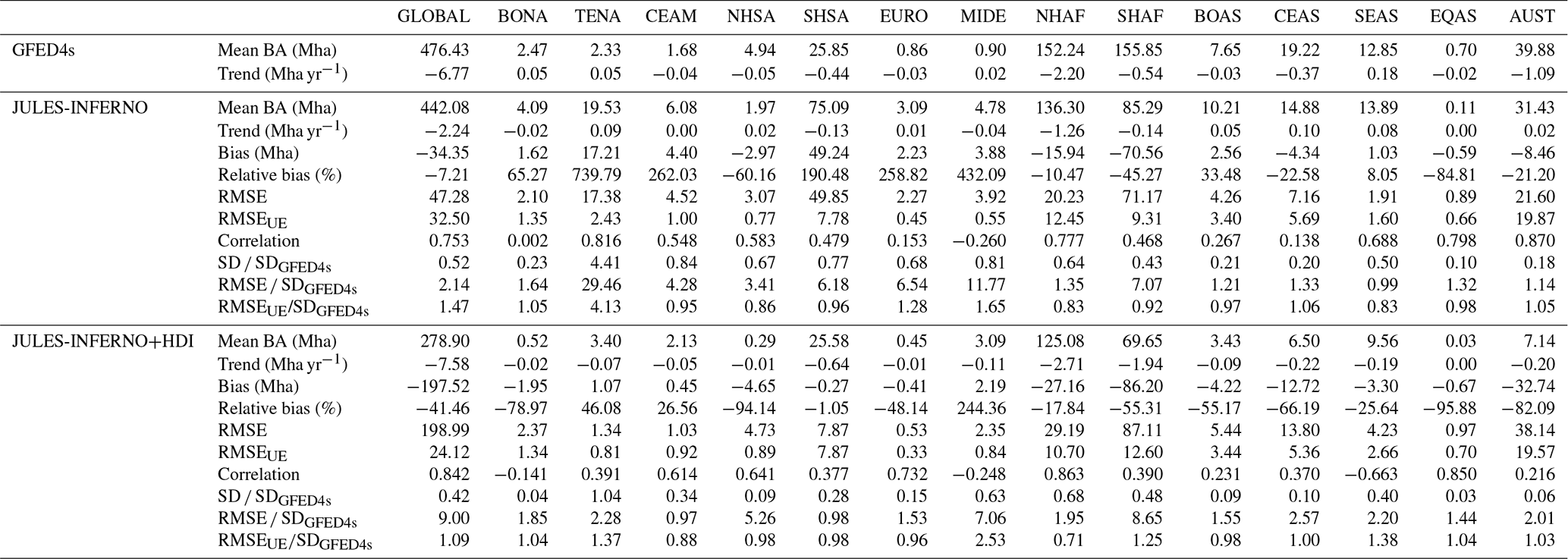
Table A2JULES-INFERNO burnt area trends (Mha yr−1) for the different GFED4s fire regions (Giglio et al., 2013) from the model sensitivity experiments. The standard error of the estimated trend, under the assumption of residual normality is shown in brackets. Values in bold represent trends that are significantly different from zero at the 95 % confidence level.
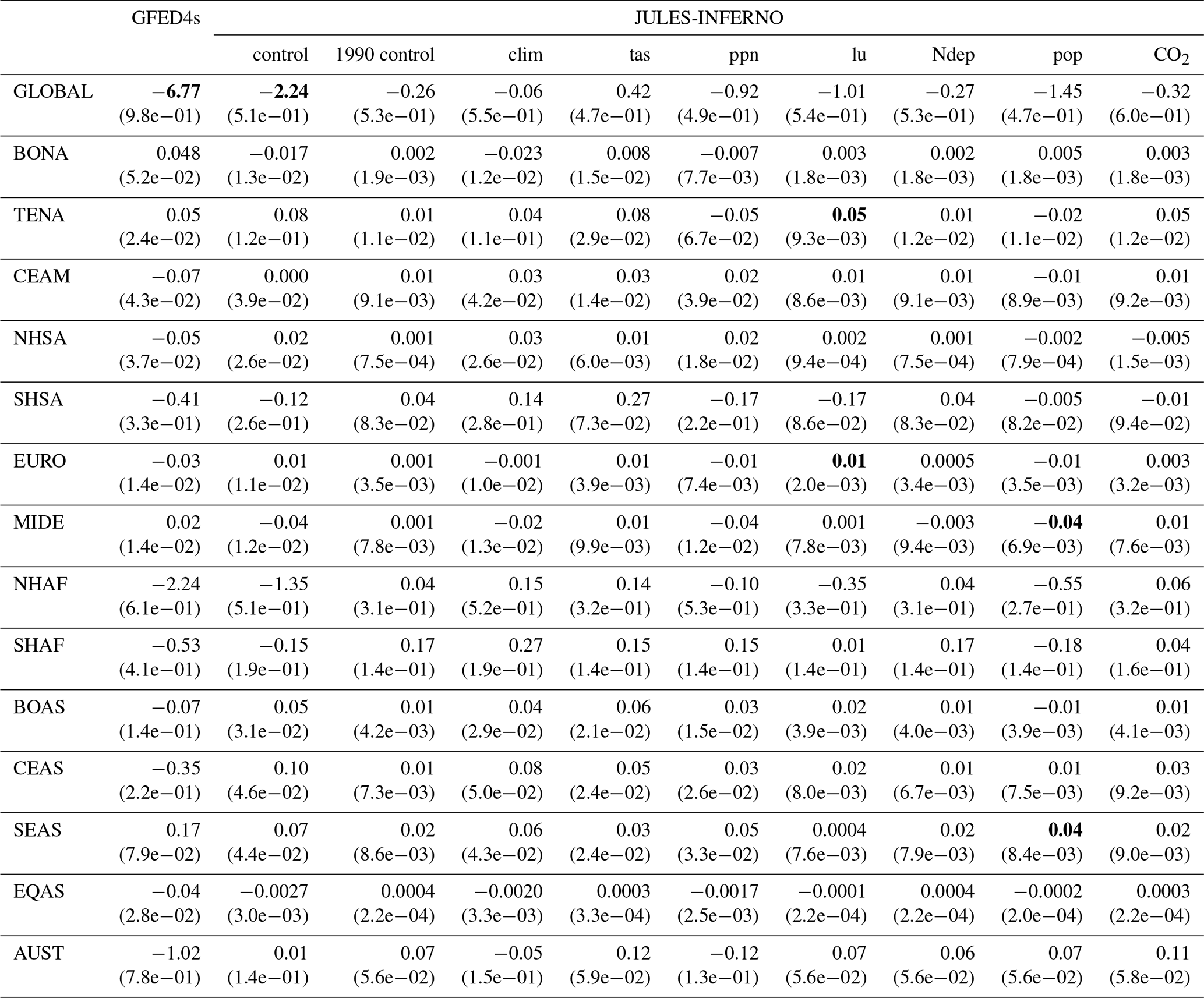
Table A3JULES-INFERNO+HDI burnt area trends (Mha yr−1) for the different GFED4s fire regions (Giglio et al., 2013) from the model sensitivity experiments. The standard error of the estimated trend, under the assumption of residual normality is shown in brackets. Values in bold represent trends that are significantly different from zero at the 95 % confidence level.
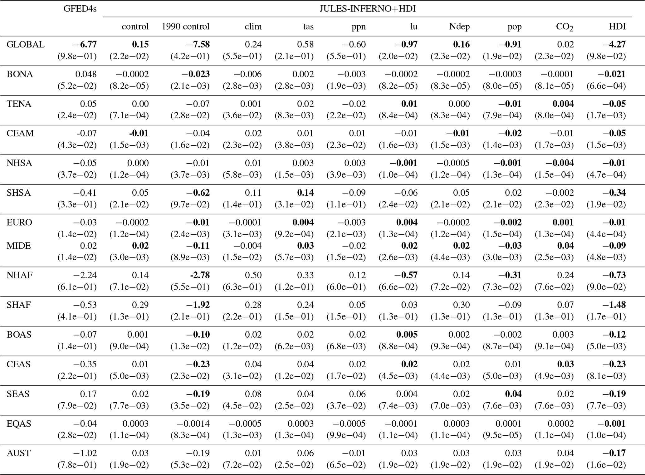
Both the model code and the files for running it are available from the Met Office Science Repository Service: https://code.metoffice.gov.uk/ (last access: 26 July 2023). Registration is required, and code is freely available subject to completion of a software license.
Details of the simulations performed: JULES simulations are compiled and run in suites developed using the Rose suite engine (MetOffice, 2022) and scheduled using the cylc workflow engine (Oliver et al., 2019). Both Rose and cylc are available under v3 of the GNU General Public License (GPL). In this framework, the suite contains the information required to extract and build the code as well as configure and run the simulations. Each suite is labelled with a unique identifier and is held in the same revision-controlled repository service in which we hold and develop the model code. This means that these suites are available to any licensed of JULES under the following suite IDs:
-
JULES-INFERNO: u-by849
-
JULES-INFERNO+HDI: u-by851
For JULES-INFERNO sensitivity experiments:
-
1990 control: u-co594
-
clim: u-cs067
-
tas: u-cs068
-
ppn: u-cs069
-
lu: u-cr440
-
Ndep: u-cr441
-
pop: u-cr442
-
CO2: u-cr443
For JULES-INFERNO+HDI sensitivity experiments:
-
1990 control: u-ct759
-
clim: u-cs070
-
tas: u-cs071
-
ppn: u-cs072
-
lu: u-cr447
-
Ndep: u-cr448
-
pop: u-cr449
-
CO2: u-cr450
-
HDI: u-cn957
JCMT led the writing of the paper and model development. All co-authors contributed to the simulation design, writing sections, performing evaluation and reviewing drafts of the paper.
At least one of the (co-)authors is a member of the editorial board of Earth System Dynamics. The peer-review process was guided by an independent editor, and the authors also have no other competing interests to declare.
Publisher's note: Copernicus Publications remains neutral with regard to jurisdictional claims made in the text, published maps, institutional affiliations, or any other geographical representation in this paper. The authors bear the ultimate responsibility for providing appropriate place names. Views expressed in the text are those of the authors and do not necessarily reflect the views of the publisher.
We would especially like to thank those who have contributed to the development of INFERNO, with a special thanks to Stéphane Mangeon for taking the first steps to develop INFERNO and the observational community, who have developed numerous datasets used in this paper to help evaluate the model.
This research and JCMT, CB, GAF, FMOC, RAB were supported by the Met Office Hadley Centre Climate Programme funded by DSIT. JCMT, GAF, and FMOC were also supported by the EU Horizon 2020 Framework Programme (CRESCENDO, grant no. 779366) and the Earth System Models for the Future (ESM2025, grant no. 101003536). CB was funded by the Met Office Climate Science for Service Partnership (CSSP) Brazil project which is supported by the Department for Science, Innovation & Technology (DSIT). DIK was supported by the Natural Environment Research Council as part of the LTSM2 TerraFIRMA project. AV was funded via the Leverhulme Centre for Wildfires, Environment and Society through the Leverhulme Trust (grant no. RC-2018-023).
This research has been supported by the EU Horizon 2020 Framework Programme, EU H2020 Societal Challenges (grant nos. 779366 and 101003536).
This paper was edited by Christian Franzke and reviewed by Vincent Verjans and one anonymous referee.
Abatzoglou, J. T. and Williams, A. P.: Impact of anthropogenic climate change on wildfire across western US forests, P. Natl. Acad. Sci. USA, 113, 11770–11775, 2016. a
Abatzoglou, J. T., Williams, A. P., Boschetti, L., Zubkova, M., and Kolden, C. A.: Global patterns of interannual climate–fire relationships, Glob. Change Biol., 24, 5164–5175, 2018. a
Andela, N. and Van Der Werf, G. R.: Recent trends in African fires driven by cropland expansion and El Nino to La Nina transition, Glob. Change Biol., 4, 791–795, 2014. a, b
Andela, N., Morton, D. C., Giglio, L., Chen, Y., van der Werf, G. R., Kasibhatla, P. S., DeFries, R. S., Collatz, G. J., Hantson, S., Kloster, S., Bachelet, D., Forrest, M., Lasslop, G., Li, F., Mangeon, S., Melton, J. R., Yue, C., and Randerson, J. T.: A human-driven decline in global burned area, Science, 356, 1356–1362, 2017. a, b, c, d, e, f, g
Andela, N., Morton, D. C., Giglio, L., Paugam, R., Chen, Y., Hantson, S., van der Werf, G. R., and Randerson, J. T.: The Global Fire Atlas of individual fire size, duration, speed and direction, Earth Syst. Sci. Data, 11, 529–552, https://doi.org/10.5194/essd-11-529-2019, 2019. a, b, c, d
Aragão, L. E. O. C., Anderson, L. O., Fonseca, M. G., Rosan, T. M., Vedovato, L. B., Wagner, F. H., Silva, C. V. J., Silva Junior, C. H. L., Arai, E., Aguiar, A. P., Barlow, J., Berenguer, E., Deeter, M. N., Domingues, L. G., Gatti, L., Gloor, M., Malhi, Y., Marengo, J. A., Miller, J. B., Phillips, O. L., and Saatchi, S.: 21st Century drought-related fires counteract the decline of Amazon deforestation carbon emissions, Nat. Commun., 9, 536, https://doi.org/10.1038/s41467-017-02771-y, 2018. a
Benjamini, Y. and Yekutieli, D.: The control of the false discovery rate in multiple testing under dependency, Ann. Stat., 29, 1165–1188, 2001. a
Best, M. J., Pryor, M., Clark, D. B., Rooney, G. G., Essery, R. L. H., Ménard, C. B., Edwards, J. M., Hendry, M. A., Porson, A., Gedney, N., Mercado, L. M., Sitch, S., Blyth, E., Boucher, O., Cox, P. M., Grimmond, C. S. B., and Harding, R. J.: The Joint UK Land Environment Simulator (JULES), model description – Part 1: Energy and water fluxes, Geosci. Model Dev., 4, 677–699, https://doi.org/10.5194/gmd-4-677-2011, 2011. a
Bhanojirao, V.: Human development report 1990: review and assessment, World Dev., 19, 1451–1460, 1991. a, b
Blackford, K. R., Kasoar, M., Burton, C., Burke, E., Prentice, I. C., and Voulgarakis, A.: INFERNO-peat v1.0.0: a representation of northern high-latitude peat fires in the JULES-INFERNO global fire model, Geosci. Model Dev., 17, 3063–3079, https://doi.org/10.5194/gmd-17-3063-2024, 2024. a
Bowman, D. M., Kolden, C. A., Abatzoglou, J. T., Johnston, F. H., van der Werf, G. R., and Flannigan, M.: Vegetation fires in the Anthropocene, Nat. Rev. Earth Environ., 1, 500–515, 2020. a
Burton, C., Betts, R., Cardoso, M., Feldpausch, T. R., Harper, A., Jones, C. D., Kelley, D. I., Robertson, E., and Wiltshire, A.: Representation of fire, land-use change and vegetation dynamics in the Joint UK Land Environment Simulator vn4.9 (JULES), Geosci. Model Dev., 12, 179–193, https://doi.org/10.5194/gmd-12-179-2019, 2019. a, b, c, d, e
Burton, C., Betts, R. A., Jones, C. D., Feldpausch, T. R., Cardoso, M., and Anderson, L. O.: El Niño Driven Changes in Global Fire 2015/16, Front. Earth Sci., 8, 199, https://doi.org/10.3389/feart.2020.00199, 2020. a
Burton, C. A., Kelley, D. I., Burke, E., Mathison, C., Jones, C. D., Betts, R. A., Robertson, E., Teixeira, J. C., Cardoso, M., and Anderson, L. O.: Fire weakens land carbon sinks before 1.5 °C, Nat. Geosci., 17, 1108–1114, 2024. a
Carreiras, M., Ferreira, A. J. D., Valente, S., Fleskens, L., Gonzales-Pelayo, Ó., Rubio, J. L., Stoof, C. R., Coelho, C. O. A., Ferreira, C. S. S., and Ritsema, C. J.: Comparative analysis of policies to deal with wildfire risk, Land Degrad. Dev., 25, 92–103, 2014. a, b
Cecil, D.: LIS/OTD 0.5 Degree High Resolution Monthly Climatology (HRMC) V2.3.2015, NASA Global Hydrometeorology Resource Center DAAC [data set], https://doi.org/10.5067/LIS/LIS-OTD/DATA303, 2006. a
Chergui, B., Fahd, S., Santos, X., and Pausas, J. G.: Socioeconomic factors drive fire-regime variability in the Mediterranean Basin, Ecosystems, 21, 619–628, 2018. a
Christian, H. J., Blakeslee, R. J., Boccippio, D. J., Boeck, W. L., Buechler, D. E., Driscoll, K. T., Goodman, S. J., Hall, J. M., Koshak, W. J., Mach, D. M., and Stewart, M. F.: Global frequency and distribution of lightning as observed from space by the Optical Transient Detector, J. Geophys. Res.-Atmos., 108, 4-1–4-15, 2003. a
Chuvieco, E., Pettinari, M. L., Koutsias, N., Forkel, M., Hantson, S., and Turco, M.: Human and climate drivers of global biomass burning variability, Sci. Total Environ., 779, 146361, https://doi.org/10.1016/j.scitotenv.2021.146361, 2021. a, b
Clark, D. B., Mercado, L. M., Sitch, S., Jones, C. D., Gedney, N., Best, M. J., Pryor, M., Rooney, G. G., Essery, R. L. H., Blyth, E., Boucher, O., Harding, R. J., Huntingford, C., and Cox, P. M.: The Joint UK Land Environment Simulator (JULES), model description – Part 2: Carbon fluxes and vegetation dynamics, Geosci. Model Dev., 4, 701–722, https://doi.org/10.5194/gmd-4-701-2011, 2011. a
Cox, P.: Description of the “TRIFFID” Dynamic Global Vegetation Mode, Met Office, https://www.paleo.bristol.ac.uk/UM_Docs/UM_Technical_Documents/HCTN_24_TRIFFID.pdf (last access: 16 June 2026), 2001. a
Cox, P., Betts, R., Jones, C., Spall, S., and Totterdell, I.: Acceleration of global warming due to carbon-cycle feedbacks in a coupled climate model, Nature, 408, 184–187, 2000. a
Curt, T. and Frejaville, T.: Wildfire policy in Mediterranean France: how far is it efficient and sustainable?, Risk Anal., 38, 472–488, 2018. a, b, c
Eyring, V., Bony, S., Meehl, G. A., Senior, C. A., Stevens, B., Stouffer, R. J., and Taylor, K. E.: Overview of the Coupled Model Intercomparison Project Phase 6 (CMIP6) experimental design and organization, Geosci. Model Dev., 9, 1937–1958, https://doi.org/10.5194/gmd-9-1937-2016, 2016. a
Field, R. D., Spessa, A. C., Aziz, N. A., Camia, A., Cantin, A., Carr, R., de Groot, W. J., Dowdy, A. J., Flannigan, M. D., Manomaiphiboon, K., Pappenberger, F., Tanpipat, V., and Wang, X.: Development of a Global Fire Weather Database, Nat. Hazards Earth Syst. Sci., 15, 1407–1423, https://doi.org/10.5194/nhess-15-1407-2015, 2015. a
Ford, A. E., Harrison, S. P., Kountouris, Y., Millington, J. D., Mistry, J., Perkins, O., Rabin, S. S., Rein, G., Schreckenberg, K., Smith, C. and Smith, T. E.: Modelling human-fire interactions: combining alternative perspectives and approaches, Frontiers in Environmental Science, 9, 649835, https://doi.org/10.3389/fenvs.2021.649835, 2021. a, b, c
Forkel, M., Andela, N., Harrison, S. P., Lasslop, G., van Marle, M., Chuvieco, E., Dorigo, W., Forrest, M., Hantson, S., Heil, A., Li, F., Melton, J., Sitch, S., Yue, C., and Arneth, A.: Emergent relationships with respect to burned area in global satellite observations and fire-enabled vegetation models, Biogeosciences, 16, 57–76, https://doi.org/10.5194/bg-16-57-2019, 2019. a, b, c
Giglio, L., Randerson, J. T., and Van Der Werf, G. R.: Analysis of daily, monthly, and annual burned area using the fourth-generation global fire emissions database (GFED4), J. Geophys. Res.-Biogeo., 118, 317–328, 2013. a, b, c, d, e, f, g
Goldewijk, K. K., Dekker, S. C., and van Zanden, J. L.: Per-capita estimations of long-term historical land use and the consequences for global change research, J. Land Use Sci., 12, 313–337, https://doi.org/10.1080/1747423X.2017.1354938, 2017. a
Goss, M., Swain, D. L., Abatzoglou, J. T., Sarhadi, A., Kolden, C. A., Williams, A. P., and Diffenbaugh, N. S.: Climate change is increasing the likelihood of extreme autumn wildfire conditions across California, Environ. Res. Lett., 15, 094016, https://doi.org/10.1088/1748-9326/ab83a7, 2020. a
Haas, O., Prentice, I. C., and Harrison, S. P.: Global environmental controls on wildfire burnt area, size, and intensity, Environ. Res. Lett., 17, 065004, https://doi.org/10.1088/1748-9326/ac6a69, 2022. a
Haas, O., Prentice, I. C., and Harrison, S. P.: Wildfires on a changing planet, Nat. Commun., 17, 1599, https://doi.org/10.1038/s41467-025-68176-4, 2026. a
Harris, I., Jones, P. D., Osborn, T. J., and Lister, D. H.: Updated high-resolution grids of monthly climatic observations – the CRU TS3. 10 Dataset, Int. J. Climatol., 34, 623–642, 2014. a
Hickel, J.: The sustainable development index: Measuring the ecological efficiency of human development in the anthropocene, Ecol. Econ., 167, 106331, https://doi.org/10.1016/j.ecolecon.2019.05.011, 2020. a, b
Jacobson, M., Smith, H., Huber-Stearns, H. R., Davis, E. J., Cheng, A. S., and Deak, A.: Comparing social constructions of wildfire risk across media, government, and participatory discourse in a Colorado fireshed, J. Risk Res., 25, 697–714, 2022. a, b
Jones, M. W., Abatzoglou, J. T., Veraverbeke, S., Andela, N., Lasslop, G., Forkel, M., Smith, A. J., Burton, C., Betts, R. A., van der Werf, G. R., and Sitch, S.: Global and regional trends and drivers of fire under climate change, Rev. Geophys., 3, e2020RG000726, https://doi.org/10.1029/2020RG000726, 2022. a, b
Jones, M. W., Kelley, D. I., Burton, C. A., Di Giuseppe, F., Barbosa, M. L. F., Brambleby, E., Hartley, A. J., Lombardi, A., Mataveli, G., McNorton, J. R., Spuler, F. R., Wessel, J. B., Abatzoglou, J. T., Anderson, L. O., Andela, N., Archibald, S., Armenteras, D., Burke, E., Carmenta, R., Chuvieco, E., Clarke, H., Doerr, S. H., Fernandes, P. M., Giglio, L., Hamilton, D. S., Hantson, S., Harris, S., Jain, P., Kolden, C. A., Kurvits, T., Lampe, S., Meier, S., New, S., Parrington, M., Perron, M. M. G., Qu, Y., Ribeiro, N. S., Saharjo, B. H., San-Miguel-Ayanz, J., Shuman, J. K., Tanpipat, V., van der Werf, G. R., Veraverbeke, S., and Xanthopoulos, G.: State of Wildfires 2023–2024, Earth Syst. Sci. Data, 16, 3601–3685, https://doi.org/10.5194/essd-16-3601-2024, 2024. a, b
Kasischke, E. S. and Turetsky, M. R.: Recent changes in the fire regime across the North American boreal region – Spatial and temporal patterns of burning across Canada and Alaska, Geophys. Res. Lett., 33, https://doi.org/10.1029/2006GL025677, 2006. a
Kelley, D. I., Bistinas, I., Whitley, R., Burton, C., Marthews, T. R., and Dong, N.: How contemporary bioclimatic and human controls change global fire regimes, Nat. Clim. Change, 9, 690–696, 2019. a, b
Kirillina, K., Shvetsov, E. G., Protopopova, V. V., Thiesmeyer, L., and Yan, W.: Consideration of anthropogenic factors in boreal forest fire regime changes during rapid socio-economic development: case study of forestry districts with increasing burnt area in the Sakha Republic, Russia, Environ. Res. Lett., 15, 035009, https://doi.org/10.1088/1748-9326/ab6c6e, 2020. a
Klauenberg, K., Wübbeler, G., Mickan, B., Harris, P., and Elster, C.: A tutorial on Bayesian normal linear regression, Metrologia, 52, 878, https://doi.org/10.1088/0026-1394/52/6/878, 2015. a
Klein Goldewijk, K., Beusen, A., Doelman, J., and Stehfest, E.: Anthropogenic land use estimates for the Holocene – HYDE 3.2, Earth Syst. Sci. Data, 9, 927–953, https://doi.org/10.5194/essd-9-927-2017, 2017. a
Kummu, M., Taka, M., and Guillaume, J. H.: Gridded global datasets for gross domestic product and Human Development Index over 1990–2015, Sci. Data, 5, 180004, https://doi.org/10.1038/sdata.2018.4, 2018. a, b, c
Li, F., Levis, S., and Ward, D. S.: Quantifying the role of fire in the Earth system – Part 1: Improved global fire modeling in the Community Earth System Model (CESM1), Biogeosciences, 10, 2293–2314, https://doi.org/10.5194/bg-10-2293-2013, 2013. a
Li, F., Song, X., Harrison, S. P., Marlon, J. R., Lin, Z., Leung, L. R., Schwinger, J., Marécal, V., Wang, S., Ward, D. S., Dong, X., Lee, H., Nieradzik, L., Rabin, S. S., and Séférian, R.: Evaluation of global fire simulations in CMIP6 Earth system models, Geosci. Model Dev., 17, 8751–8771, https://doi.org/10.5194/gmd-17-8751-2024, 2024. a, b
Mangeon, S., Voulgarakis, A., Gilham, R., Harper, A., Sitch, S., and Folberth, G.: INFERNO: a fire and emissions scheme for the UK Met Office's Unified Model, Geosci. Model Dev., 9, 2685–2700, https://doi.org/10.5194/gmd-9-2685-2016, 2016. a, b, c, d, e
Marlon, J. R., Bartlein, P. J., Carcaillet, C., Gavin, D. G., Harrison, S. P., Higuera, P. E., Joos, F., Power, M., and Prentice, I.: Climate and human influences on global biomass burning over the past two millennia, Nat. Geosci., 1, 697–702, 2008. a
Mathison, C., Burke, E., Hartley, A. J., Kelley, D. I., Burton, C., Robertson, E., Gedney, N., Williams, K., Wiltshire, A., Ellis, R. J., Sellar, A. A., and Jones, C. D.: Description and evaluation of the JULES-ES set-up for ISIMIP2b, Geosci. Model Dev., 16, 4249–4264, https://doi.org/10.5194/gmd-16-4249-2023, 2023. a
MetOffice: Rose suite engine, https://metomi.github.io/rose/doc/html/index.html (last access: 16 June 2026), 2022. a
Miranda-Lescano, R., Muinelo-Gallo, L., and Roca-Sagalés, O.: Human development and decentralization: The importance of public health expenditure, Ann. Public Coop. Econ., 94, 191–219, 2023. a
Mourão, P. R. and Martinho, V. D.: The choices of the fire – Debating socioeconomic determinants of the fires observed at Portuguese municipalities, Forest Policy Econ., 43, 29–40, 2014. a, b
Nepstad, D., McGrath, D., Stickler, C., Alencar, A., Azevedo, A., Swette, B., Bezerra, T., DiGiano, M., Shimada, J., Seroa da Motta, R., and Armijo, E.: Slowing Amazon deforestation through public policy and interventions in beef and soy supply chains, Science, 344, 1118–1123, 2014. a
Nikolakis, W. and Roberts, E.: Wildfire governance in a changing world: Insights for policy learning and policy transfer, RHCPP, 13, 144–164, 2022. a, b, c
Oliver, H., Shin, M., Matthews, D., Sanders, O., Bartholomew, S., Clark, A., Fitzpatrick, B., van Haren, R., Hut, R., and Drost, N.: Workflow automation for cycling systems, Comput. Sci. Eng., 21, 7–21, 2019. a
Pandey, P., Huidobro, G., Lopes, L. F., Ganteaume, A., Ascoli, D., Colaco, C., Xanthopoulos, G., Giannaros, T. M., Gazzard, R., Boustras, G., and Steelman, T.: A global outlook on increasing wildfire risk: Current policy situation and future pathways, Trees For. People, 14, 100431, https://doi.org/10.1016/j.tfp.2023.100431, 2023. a
Pechony, O. and Shindell, D.: Fire parameterization on a global scale, J. Geophys. Res.-Atmos., 114, D16115, https://doi.org/10.1029/2009JD011927, 2009. a, b
Perkins, O., Kasoar, M., Voulgarakis, A., Smith, C., Mistry, J., and Millington, J. D. A.: A global behavioural model of human fire use and management: WHAM! v1.0, Geosci. Model Dev., 17, 3993–4016, https://doi.org/10.5194/gmd-17-3993-2024, 2024. a, b
Prestemon, J. P., Butry, D. T., Abt, K. L., and Sutphen, R.: Net benefits of wildfire prevention education efforts, Forest Sci., 56, 181–192, 2010. a
Rabin, S. S., Melton, J. R., Lasslop, G., Bachelet, D., Forrest, M., Hantson, S., Kaplan, J. O., Li, F., Mangeon, S., Ward, D. S., Yue, C., Arora, V. K., Hickler, T., Kloster, S., Knorr, W., Nieradzik, L., Spessa, A., Folberth, G. A., Sheehan, T., Voulgarakis, A., Kelley, D. I., Prentice, I. C., Sitch, S., Harrison, S., and Arneth, A.: The Fire Modeling Intercomparison Project (FireMIP), phase 1: experimental and analytical protocols with detailed model descriptions, Geosci. Model Dev., 10, 1175–1197, https://doi.org/10.5194/gmd-10-1175-2017, 2017. a, b, c
Ramdas, A., García Trillos, N., and Cuturi, M.: On wasserstein two-sample testing and related families of nonparametric tests, Entropy, 19, 47, https://doi.org/10.3390/e19020047, 2017. a
Randerson, J., Chen, Y., Van Der Werf, G., Rogers, B., and Morton, D.: Global burned area and biomass burning emissions from small fires, J. Geophys. Res.-Biogeo., 117, G04012, https://doi.org/10.1029/2012JG002128, 2012. a
Rideout, D. B., Wei, Y., Kirsch, A., and Kernohan, N.: STARFire: Strategic budgeting and planning for wildland fire management, Park Sci., 32, 34–41, 2017. a
Riley, K. L., Williams, A. P., Urbanski, S. P., Calkin, D. E., Short, K. C., and O'Connor, C. D.: Will landscape fire increase in the future? A systems approach to climate, fire, fuel, and human drivers, Curr. Pollut. Rep., 5, 9–24, 2019. a, b
Rizzo, L. V. and Rizzo, M. C. F.: Wildfire smoke and health impacts: a narrative review, Jornal de Pediatria, https://doi.org/10.1016/j.jped.2024.11.006, 2024. a
Roy, A., Dutta, T., Li, Y., and Dong, X.: Human development at the cost of the environment? – an application of planetary pressures – adjusted human development index in the lens of planetary boundaries, Environ. Sci. Pollut. Res., 30, 32383–32405, 2023. a, b
Sellar, A. A., Jones, C. G., Mulcahy, J. P., Tang, Y., Yool, A., Wiltshire, A., O'Connor, F. M., Stringer, M., Hill, R., Palmieri, J., Woodward, S., de Mora, L., Kuhlbrodt, T., Rumbold, S. T., Kelley, D. I., Ellis, R., Johnson, C. E., Walton, J., Abraham, N. L., Andrews, M. B., Andrews, T., Archibald, A. T., Berthou, S., Burke, E., Blockley, E., Carslaw, K., Dalvi, M., Edwards, J., Folberth, G. A., Gedney, N., Griffiths, P. T., Harper, A. B., Hendry, M. A., Hewitt, A. J., Johnson, B., Jones, A., Jones, C. D., Keeble, J., Liddicoat, S., Morgenstern, O., Parker, R. J., Predoi, V., Robertson, E., Siahaan, A., Smith, R. S., Swaminathan, R., Woodhouse, M. T., Zeng, G., and Zerroukat, M.: UKESM1: Description and Evaluation of the U.K. Earth System Model, J. Adv. Model. Earth Sy., 11, 4513–4558, https://doi.org/10.1029/2019MS001739, 2019a. a
Sellar, A. A., Jones, C. G., Mulcahy, J. P., Tang, Y., Yool, A., Wiltshire, A., O'Connor, F. M., Stringer, M., Hill, R., Palmieri, J., Woodward, S., de Mora, L., Kuhlbrodt, T., Rumbold, S. T., Kelley, D. I., Ellis, R., Johnson, C. E., Walton, J., Abraham, N. L., Andrews, M. B., Andrews, T., Archibald, A. T., Berthou, S., Burke, E., Blockley, E., Carslaw, K., Dalvi, M., Edwards, J., Folberth, G. A., Gedney, N., Griffiths, P. T., Harper, A. B., Hendry, M. A., Hewitt, A. J., Johnson, B., Jones, A., Jones, C. D., Keeble, J., Liddicoat, S., Morgenstern, O., Parker, R. J., Predoi, V., Robertson, E., Siahaan, A., Smith, R. S., Swaminathan, R., Woodhouse, M. T., Zeng, G., and Zerroukat, M.: UKESM1: Description and evaluation of the UK Earth System Model, J. Adv. Model. Earth Sy., 11, 4513–4558, 2019b. a
Silva Junior, C. H., Pessôa, A. C., Carvalho, N. S., Reis, J. B., Anderson, L. O., and Aragão, L. E.: The Brazilian Amazon deforestation rate in 2020 is the greatest of the decade, Nat. Ecol. Evol., 5, 144–145, 2021. a
Stocks, B. J., Mason, J. A., Todd, J. B., Bosch, E. M., Wotton, B. M., Amiro, B. D., Flannigan, M. D., Hirsch, K. G., Logan, K. A., Martell, D. L., and Skinner, W. R: Large forest fires in Canada, 1959–1997, J. Geophys. Res.-Atmos., 107, FFR 5-1–FFR 5-12, https://doi.org/10.1029/2001JD000484, 2002. a
Sullivan, A., Baker, E., and Kurvits, T. (Eds.): Spreading like Wildfire: The Rising Threat of Extraordinary Landscape Fires., United Nations Environment Programme (UNEP), https://wedocs.unep.org/handle/20.500.11822/38372 (last access: 16 June 2026), 2022. a, b
Teckentrup, L., Harrison, S. P., Hantson, S., Heil, A., Melton, J. R., Forrest, M., Li, F., Yue, C., Arneth, A., Hickler, T., Sitch, S., and Lasslop, G.: Response of simulated burned area to historical changes in environmental and anthropogenic factors: a comparison of seven fire models, Biogeosciences, 16, 3883–3910, https://doi.org/10.5194/bg-16-3883-2019, 2019. a
Teixeira, J. C., Folberth, G. A., O'Connor, F. M., Unger, N., and Voulgarakis, A.: Coupling interactive fire with atmospheric composition and climate in the UK Earth System Model, Geosci. Model Dev., 14, 6515–6539, https://doi.org/10.5194/gmd-14-6515-2021, 2021. a, b, c
Türe, C.: A methodology to analyse the relations of ecological footprint corresponding with human development index: eco-sustainable human development index, Int. J. Sustain. Dev. World Ecol., 20, 9–19, 2013. a, b
Veraverbeke, S., Rogers, B. M., Goulden, M. L., Jandt, R. R., Miller, C. E., Wiggins, E. B., and Randerson, J. T.: Lightning as a major driver of recent large fire years in North American boreal forests, Nat. Clim. Change, 7, 529–534, 2017. a
Verjans, V., Franzke, C. L., Lee, S.-S., Kim, I.-W., Tilmes, S., Lawrence, D. M., Vitt, F., and Li, F.: Quantifying CO2 forcing effects on lightning, wildfires, and climate interactions, Sci. Adv., 11, eadt5088, https://doi.org/10.1126/sciadv.adt5088, 2025. a
Viovy, N.: CRUNCEP version 7-atmospheric forcing data for the community land model, Research Data Archive at the National Center for Atmospheric Research, Computational and Information Systems Laboratory [data set], https://doi.org/10.5065/PZ8F-F017, 2018. a
Vitolo, C., Di Giuseppe, F., Barnard, C., Coughlan, R., San-Miguel-Ayanz, J., Libertá, G., and Krzeminski, B.: ERA5-based global meteorological wildfire danger maps, Sci. Data, 7, 216, https://doi.org/10.1038/s41597-020-0554-z, 2020. a
Williams, A. P., Abatzoglou, J. T., Gershunov, A., Guzman-Morales, J., Bishop, D. A., Balch, J. K., and Lettenmaier, D. P.: Observed impacts of anthropogenic climate change on wildfire in California, Earth's Future, 7, 892–910, 2019. a
Williams, K. D., Copsey, D., Blockley, E. W., Bodas-Salcedo, A., Calvert, D., Comer, R., Davis, P., Graham, T., Hewitt, H. T., Hill, R., Hyder, P., Ineson, S., Johns, T. C., Keen, A. B., Lee, R. W., Megann, A., Milton, S. F., Rae, J. G. L., Roberts, M. J., Scaife, A. A., Schiemann, R., Storkey, D., Thorpe, L., Watterson, I. G., Walters, D. N., West, A., Wood, R. A., Woollings, T., and Xavier, P. K.: The Met Office global coupled model 3.0 and 3.1 (GC3.0 and GC3.1) configurations, J. Adv. Model. Earth Syst., 10, 357–380, 2018. a
Yue, C., Ciais, P., Cadule, P., Thonicke, K., Archibald, S., Poulter, B., Hao, W. M., Hantson, S., Mouillot, F., Friedlingstein, P., Maignan, F., and Viovy, N.: Modelling the role of fires in the terrestrial carbon balance by incorporating SPITFIRE into the global vegetation model ORCHIDEE – Part 1: simulating historical global burned area and fire regimes, Geosci. Model Dev., 7, 2747–2767, https://doi.org/10.5194/gmd-7-2747-2014, 2014. a
Zou, Y., Wang, Y., Ke, Z., Tian, H., Yang, J., and Liu, Y.: Development of a REgion-specific ecosystem feedback fire (RESFire) model in the Community Earth System Model, J. Adv. Model. Earth Sy., 11, 417–445, 2019. a