Atmospheric river trajectories organise along a global transport network

Atmospheric rivers (ARs) transport vast amounts of water vapor and cause weather extremes. However, they have typically been studied as isolated events rather than as components of a global transport system. By mapping ARs worldwide, we reveal that their transport is organized along a sparse set of preferred pathways forming a global network. Recognizing ARs as a globally interconnected system is highly relevant, not only for advancing atmospheric science but also for improving forecasts of extreme precipitation, droughts, and polar ice melt under climate change. Beyond the familiar storm tracks, we identify hubs of pronounced vapor transport changes and demonstrate that polar regions act as structural accumulation regions for persistent ARs. ARs preferentially travel along circumglobal atmospheric highways shaped by teleconnection patterns and circulation regimes, providing new opportunities for AR prediction. While previous research recognized only five AR basins, we uncover a larger, hierarchically organized set of interconnected basins that provides a more comprehensive understanding of how regional AR hotspots are embedded within large-scale flow. The global AR transport network links synoptic storms to planetary circulation, illuminating hidden pathways in the global water cycle.

1 Introduction

Atmospheric flows of moisture govern the global availability of fresh water, control land surface processes, and can cause considerable hazards and impacts. With climate change intensifying the global water cycle and exacerbating both floods and droughts globally (Held and Soden, 2006), our understanding of the intricate processes that connect moisture sinks and sources around the globe becomes ever-more vital (Rockström et al., 2023). Among the various synoptic-scale phenomena that distribute freshwater globally, atmospheric rivers (ARs) – narrow and long channels of anomalously high water vapor transport in the lower atmosphere (Zhu and Newell, 1994; Gimeno et al., 2016) – are the main mechanism of meridional moisture transport in the mid-latitudes. ARs transport 90 % of poleward moisture into the mid-latitudes while covering less than 10 % of Earth's surface (Gimeno et al., 2014). Their influence on the high-dimensional Earth system is truly multi-faceted: they affect global heat budgets (Scholz and Lora, 2024), contribute to tropical moisture transport (Park and Son, 2024), cause hydrological extremes (Francis et al., 2024), drive Arctic glacier melt (Wang et al., 2024), and reduce Antarctic sea ice (Liang et al., 2023).

Despite growing recognition of ARs as part of large-scale teleconnection patterns (Pan et al., 2024; Garaboa-Paz et al., 2017), recent studies still fall short of considering them as components of a dynamic, interconnected global moisture transport system. Instead, most research employs a local, Eulerian approach and focuses on a specific region (Ramos et al., 2016; Ryoo et al., 2015; Ye et al., 2020; Viale et al., 2018; Pan and Lu, 2020). While this approach is essential to better understand local AR hazards and impacts, it does not consider and thus likely fragments AR trajectories. Fewer studies have investigated AR dynamics at fully global scale, providing valuable insights on AR life cycles, i.e., where they are generated, where they terminate, and how most of their activity is concentrated along the mid-latitudinal storm tracks (Guan and Waliser, 2015; Gimeno et al., 2020). Both at the regional and global scale, previous work often relies on conventional composite analysis, complemented by Lagrangian dispersion models which are computationally expensive at larger spatial scales (Stohl and James, 2004; Tuinenburg and Staal, 2020; Gimeno et al., 2020). As a consequence, our understanding of how planetary-scale atmospheric moisture transport emerges from specific synoptic-scale phenomena (such as ARs) remains limited, leaving central questions about global AR dynamics unanswered:

1. Beyond the familiar regions of high AR activity along the mid-latitudinal storm tracks, where do ARs tend to strengthen or weaken their water vapor transport, and where do they structurally converge to?

2. How is AR transport structured within planetary-scale teleconnection patterns? Is there a global “highway system” of critical conduits that steer AR transport?

3. Is it sufficient to understand AR transport along the previously recognized five main basins (Park et al., 2023), or do these contain an internal structure that helps us to better understand how regional AR hotspots are embedded within large-scale flow?

To tackle these questions, we introduce a novel transport network framework for AR trajectories. Unlike conventional approaches, the network architecture highlights connectivity and reveals emergent transport pathways across scales (Coscia, 2021). In contrast to the Eulerian approach employed in the vast majority of previous studies, this framework considers ARs as individual moisture streams rather than localized disconnected events. A complex network is a set of interconnected nodes whose non-random, often clustered structure reflects the intricate organization of the underlying complex system. By understanding global moisture transport through ARs as a network, we can identify important hubs of high AR activity as central nodes, key moisture conduits as preferential edges, and large-scale transport basins as node communities. This view mirrors terrestrial river networks, where branching tributaries organize water flow across scales (LeGrande et al., 2024). The success of networks in climate is underlined by recent applications which have provided novel insights into teleconnection patterns (Runge et al., 2015; Boers et al., 2019; Liu et al., 2023), forecasting (Ludescher et al., 2021), interactions between synoptic-scale features (Gupta et al., 2021), synchronization of extremes (Vallejo-Bernal et al., 2023), moisture recycling hubs (Wunderling et al., 2022), and propagation pathways of extreme precipitation (Malik et al., 2010; Li et al., 2024). Still, most climate network studies rely on correlations, which may give rise to spurious links (Haas et al., 2023) and do not represent physical links. Lagrangian flow networks overcome some of these limitations by explicitly tracing fluid parcels and have enriched our understanding of atmospheric circulation (Molkenthin et al., 2014; Gelbrecht et al., 2017; Ser-Giacomi et al., 2015c). Yet, they remain computationally heavy and agnostic to the specific transport mechanism. This distinction matters: different mechanisms of atmospheric moisture transport exhibit varying hazard potentials, degrees of predictability, and responses to a changing climate (Gimeno et al., 2016).

Instead of tracking fluid parcels, the approach introduced here preserves the physical interpretability of the underlying transport phenomenon (Prein et al., 2023), and instead of relying on a purely statistical correlation-based approach, we encode the AR contribution to the global water cycle through a physical transport network. The objective of this study is to introduce the developed framework and demonstrate its scope through global AR transport analysis. We showcase that it holds potential for AR prediction and actionable science, clearly disentangling AR moisture flows that are critical for water resource management and hazard mitigation. By capturing the global connectivity of AR dynamics, it uniquely enables us to address open questions about how synoptic-scale weather systems collectively shape planetary-scale moisture transport.

2 Methods

2.1 Atmospheric river catalogs

We extract AR trajectories from two global state-of-the-art catalogs: the PIK Atmospheric River Trajectories version 1.0 (PIKART-1.0) catalog (Vallejo-Bernal et al., 2025a) and the Tracking Atmospheric Rivers Globally as Elongated Targets Version 4 (tARget-4) catalog (Guan and Waliser, 2015; Guan et al., 2018; Guan and Waliser, 2019, 2024). Both catalogs are based on ERA5 reanalysis data and record 84 years (1940–2023) of AR activity with high spatiotemporal resolution of 0.5° and 6 h. As a general note of caution, we would like to stress that the ERA5 extension prior to 1979 (1940–1979) is known to suffer from reduced data quality, especially before the mid 1950s (Hersbach et al., 2020). The overall structure of the global atmospheric river transport network (ARTN) is qualitatively recovered for the pre-1979 period and for an ARTN derived from the MERRA2-based version of the PIKART-1.0 catalog (Fig. S1). Quantitatively, the pre- and post-1979 ERA5 networks share a Jaccard edge overlap of 0.69 and a Spearman rank correlation of 0.87 computed from edge weights on common edges, while the post-1979 ERA5 and MERRA2 networks agree more modestly (Jaccard 0.50, ρ=0.65).

PIKART-1.0 (Vallejo-Bernal et al., 2025a) employs advanced image processing techniques to detect ARs: it identifies ARs as endogenous synoptic-scale IVT anomalies using a top-hat reconstruction technique (Xu et al., 2020a), without relying on globally fixed magnitude thresholds, and allowing the detection scheme to adapt to regionally and temporally varying atmospheric moisture content. tARget-4 (Guan and Waliser, 2024, 2019, 2015) combines relative IVT thresholds with a fixed lower IVT limit. Both algorithms track ARs based on distinct criteria for spatial proximity and morphological similarity of AR shapes, and include physically-meaningful post-processing that filters detections based on geometric and transport-related criteria. The global AR distributions produced by both catalogs have been found to agree on important key regions but yield differing frequencies in regions with anomalous atmospheric moisture content, such as the tropics, mountainous regions, and the poles (Vallejo-Bernal et al., 2025a). Both are included in the Atmospheric River Tracking Method Intercomparison Project (ARTMIP) database (Shields et al., 2018; Rutz et al., 2019).

2.2 Network construction

Atmospheric river transport networks (ARTNs) are a mathematical representation of AR transport patterns that allows visualization, quantification, and modeling approaches. The observational transport patterns that define the ARTN's topology are extracted from a sufficiently large set of spatiotemporal AR trajectories. They consequently adopt a Lagrangian perspective where each AR is tracked along its trajectory. Nodes in the network are given by geographical locations. Edges encode the observed transport patterns. Here, we formally introduce the ARTN framework (Fig. S2).

Let $\mathcal{G}=(\mathcal{V},\mathcal{E})$ represent the directed, weighted transport network of ARs, where 𝒱 is the set of nodes corresponding to spatial grid cells, and ℰ is the set of edges representing AR trajectories traversing between nodes. Each node v_i∈𝒱 corresponds to a discrete grid cell centered at coordinates (lat_i,lon_i). The grid covers a spatial domain 𝒳 (global extent in this study). While the grid could be defined with standard rectangular latitude-longitude grid cells, this would yield significant biases towards the poles due to spherical distortions (Giammarese et al., 2024). Discrete Global Grid Systems offer a more adequate gridding approach for global analyses that minimizes cell distortions (Brooks et al., 2018). Here, we employ a hexagonal gridding scheme where the Earth is projected to an icosahedron (gnomonic projection) and tiled with hexagons (Brooks et al., 2018). Hexagonal grid cells entail reduced biases for the network measures computed here (Fig. S3) and offer a set of additional advantages (e.g., intuitive cell neighboring). Every node is thus located at the center coordinates of a hexagon at a discrete spatial resolution that corresponds to average cell areas of 86 801.78 km² (≈2.65 ° at the equator).

We define a transport event as an AR passing through two arbitrary grid cells between two consecutive time steps. To establish this definition, ARs need to be represented by a set of 2D-coordinates, i.e., a locator $\mathbf{s}=\left({\mathrm{lat}}_i,{\mathrm{lon}}_i\right)$. This central constraint allows flexibility in defining different AR locators tailored to specific research objectives, but discards information on the AR's spatial extent. In this work, most ARTNs are computed from the AR centroid, an effective geometrical locator weighted by the IVT magnitude. Alternatively, ARs could be localized by their core (the position of an AR's maximum IVT), yielding an overall consistent network topology (Fig. S4). Locating them by their head (the foremost point across the AR's axis) yields less stable trajectories (Fig. S5) and shifts the geographic distribution of AR network metrics further downstream (Fig. S6).

A directed edge e_ij∈ℰ connects node v_i to node v_j if at least one AR transport event occurs between these nodes over the observational time period. This rather permissive edge definition can be scrutinized by thresholding the AR transport matrix W (see below). For each directed edge, we calculate the transport weight w_ij as the (i,j) th entry of the transport matrix W=[w_ij]. Here, we choose w_ij to denote the number of ARs arriving at node v_j from node v_i (while it could, e.g., also reflect moisture transport or other relevant transport properties). By default, we omit self-links, i.e., $w_{ij}=\mathrm{0}\forall i=j$. Consequently, W is, by definition, an asymmetric matrix with integer entries that quantify the directed AR transport between each pair of nodes. As an important caveat to the method, some observed displacements of the AR locator result from AR deformation rather than from actual AR advancement. The higher the spatial resolution, the more of such AR movements will contribute to the respective edge weight. Omitting self-links reduces the influence of such deformations. Note that edges can generally exist between any pair of neighboring or non-neighboring nodes. As there are physical constraints to how fast ARs typically move (20–100 km h⁻¹) (Guan and Waliser, 2019; Vallejo-Bernal et al., 2025a), most edges, however, connect nodes that are spatially close to each other. If spatial resolution is too coarse (>600 km = 5.41 ° at the equator), only little meaningful trajectory information can be obtained. This can have notable effects on network metrics (Fig. S7).

From the transport matrix W, we construct the transport network 𝒢 by treating each non-zero element w_ij>0 as a directed weighted edge in the graph (similar to Ser-Giacomi et al., 2015a). Alternatively, we can generate an undirected, symmetric, weighted graph by discarding edge directions, i.e., by symmetrizing the weights such that ${\stackrel{\mathrm{̃}}{w}}_{ij}={\stackrel{\mathrm{̃}}{w}}_{ji}=w_{ij}+w_{ji}$. A directed, asymmetric, unweighted graph can be obtained by setting all nonzero entries W_ij>0 to 1. This is equivalent to thresholding the transport matrix by a transport frequency of ϵ=1. Instead, we can as well choose a more informed threshold ϵ>1, e.g., based on some notion of what is the lowest AR transport frequency that we deem sufficiently high to define a “significant” transport pattern. High threshold values will erode the network and only retain the most frequent AR pathways, potentially discarding regions rarely visited by ARs but where ARs are still a vital control on freshwater supply (Fig. S8b/d). On the other hand, choosing a low (or no) threshold value increases computational complexity and could spuriously overstress rarely traversed pathways, e.g., in the computation of centrality measures (Fig. S8a/c and Sect. 2.5). Some of the network metrics defined in Sect. 2.5 (e.g., node strength (Fig. S9a–e)) respond less sensitively to varying the threshold parameter than others (e.g., edge betweenness centrality (Fig. S9f–j)). More sophisticated approaches for network sparsification that identify an optimal value for ϵ can be tested in future studies. The resulting graph is represented as $\mathcal{G}=(\mathcal{V},\mathcal{E})$ and referred to as the AR transport network (ARTN).

Beyond the basic transport definition, edges in the ARTN $\mathcal{G}=(\mathcal{V},\mathcal{E})$ can be conditioned on additional criteria to tailor the network's construction to specific research objectives. We can define a subset of AR transport events 𝒯_C⊆𝒯, where 𝒯 is the set of all AR transport events, and 𝒯_C satisfies a criterion C. For instance, C can represent a specific temporal constraint (e.g., boreal summer), an AR property threshold (e.g., IVT≥IVT_min), or a spatial constraint (e.g., genesis within a predefined region ℛ_g). Formally, let 𝒯_C be defined as:

$$\begin{array}{}\text{(1)}& {\mathcal{T}}_C=\mathit{\{}\mathit{\tau }\in \mathcal{T}\mid C(\mathit{\tau })=\text{True}\mathit{\}}.\end{array}$$

Thus, a directed edge e_ij∈ℰ exists between nodes v_i and v_j if at least one transport event τ∈𝒯_C traverses from v_i to v_j. The transport weight $w_{ij}^c$ for this edge is computed analogously to the unconditioned case but restricted to the subset 𝒯_C. The resulting transport matrix ${\mathbf{W}}_C=\left[w_{ij}^c\right]$ defines the refined network ${\mathcal{G}}_C=(\mathcal{V},{\mathcal{E}}_C)$, where:

$$\begin{array}{}\text{(2)}& {\mathcal{E}}_C=\mathit{\{}{e}_{ij}\mid w_{ij}^c>\mathrm{0}\mathit{\}}.\end{array}$$

We construct upstream networks as a particular type of a conditioned ARTN by identifying only those segments of AR trajectories that eventually feed into a specified target region. This approach conditions AR pathways on entry into the region, retaining the portion of each trajectory leading up to and including the entry point, as well as the segment within the region.

For any conditional ARTN, thresholds have to be selected carefully as conditioning naturally reduces AR frequencies along each edge. We selected all thresholds such that they yield a comparable number of edges between different phases of a given climate oscillation (e.g., seasonality) and an overall sufficient number of edges for each upstream network.

Overall, approaches following a similar pipeline could be applied to any other synoptic-scale weather system (Prein et al., 2023).

2.3 Consensus networks

The framework developed here seamlessly integrates multiple AR catalogs. The most straightforward approach is the computation of individual ARTNs from individual catalogs and direct comparison of any derived node-, edge-, path-, or community-based property. However, we can also represent the common transport patterns found among a number of K different AR catalogs by a single ARTN. Similar to climate model ensembles, a consensus weight $w_{ij}^{\text{cons}}$ can be determined for an edge connecting nodes i and j by aggregating edge weights $w_{ij}^{\left(k\right)}$ across all K AR networks:

$$\begin{array}{}\text{(3)}& w_{ij}^{\text{cons}}=\left\{\begin{array}{ll}\frac{\mathrm{1}}{K}{\sum }_{k=\mathrm{1}}^K{w}_{ij}^{\left(k\right)},& \text{if }{w}_{ij}^{\left(k\right)}\ge \mathit{ϵ}\forall k\text{ where }{w}_{ij}^{\left(k\right)}>\mathrm{0},\\ \mathrm{0},& \text{otherwise.}\end{array}\right.\end{array}$$

with the weight threshold ϵ. This simple approach emphasizes robust transport pathways supported by multiple catalogs by excluding inconsistent connections (see Fig. S8/9). We also tested a majority vote scheme (an edge is preserved if at least 75 % of the networks agree on its existence and the edge weight is the median of the latter), as well as a rank-based consensus (within each network, edge weights are replaced by their percentile rank across all edges and an edge is preserved if its mean rank exceeds ϵ). The three considered approaches yielded overall consistent networks (Fig. S10).

2.4 Null models

We developed four null models to test whether a certain ARTN property (e.g., node strength) is significant for a given node/edge or if it could appear by chance (Fig. 1). The key idea is inspired by time series surrogates (Lancaster et al., 2018): we preserve a certain set of properties in the real ARTN and randomize others to control for the effect of the non-randomized properties. With this approach, we pose the question whether a certain observed property that characterizes global AR transport could be obtained from an ensemble of AR trajectories that move randomly without any constraints imposed by large-scale atmospheric circulation, as well as land-atmosphere-feedbacks, ocean-atmosphere coupling, and overall climate dynamics. Each set of simulated random AR trajectories gives rise to a single synthetic, random ARTN. The individual models are explained below:

• i.

  Fully Random Walker (FRW): AR trajectories are generated by performing an ensemble of random walks on a fully connected global network that has the same spatial resolution as the original ARTN. The walk starts at a randomly chosen node, and at each step, the walker moves to a randomly selected connected node (Fig. 1a).
  Preserved properties: number of AR trajectories, lifetimes.
  Null hypothesis: The value of network property 𝒳 is fully explained by the number and lengths of the observed AR trajectories (and consequently not driven by atmospheric circulation)

• ii.

  Rewired Graph (RWG): This model generates new graphs by rewiring edges in the network while approximately preserving the original distribution of node strengths. For a node v_i with s edges, a new set of edges $\stackrel{\mathrm{̃}}{s}$ is generated randomly (while preserving edge weights and in/out-directions). The new, rewired edges are constrained by spatial proximity up to a certain maximum node displacement δ to avoid unphysical edge lengths (Fig. 1b).
  Preserved properties: node strengths (approximately), large-scale connectivity structure.
  Null hypothesis: The value of network property 𝒳 is fully explained by the large-scale connectivity structure, i.e., if ARs locally followed different patterns but maintained their large-scale transport basins, 𝒳 would not change significantly.

• iii.

  Genesis-Constrained Random Walker (GCW): Same as FRW, but a walker with the mth walk length (equivalent to the lifetime of the mth AR) starts at the node identified with the genesis location of the mth AR, exactly preserving AR genesis regions (Fig. 1c).
  Preserved properties: number of AR trajectories, lifetimes, genesis locations.
  Null hypothesis: The value of network property 𝒳 is fully explained by the number and lengths of the observed AR trajectories, together with the AR genesis locations (and consequently not solely driven by atmospheric advection from these locations).

• iv.

  Termination-Constrained Random Walker (TCW): Equivalent to the GCW, but instead of genesis, termination locations are preserved. This is achieved by simulating a random walk from the node that is identified with a termination location and reversing it afterwards (Fig. 1d). Preserved properties and null hypothesis are analogous to the GCW but with termination instead of genesis.

Given a specific network property (e.g., node strength), we generate N_r=200 null model networks for each model (example realizations are shown in Fig. S11). From these, p-values are computed from the node or edge-specific distribution of the network property as the number of model realizations whose value of interest exceeds/falls below the real value. When multiple tests are applied together (e.g., in Fig. 2b–d), we control for false discovery rates using the Benjamini-Hochberg method for multiple testing (Benjamini and Hochberg, 1995). A value for the property of interest is deemed significant if it exceeds the corrected α=90 %-confidence level, unless stated otherwise. We apply the hypothesis tests in the order of how closely the simulated network matches the real ARTN. Overall, the displayed null models underscore the systematic structure and sparseness of the real ARTN.

2.5 Network analysis

Here, we define the measures employed in this study for network analysis. Most of them are covered in greater depth in standard text books on graph theory, e.g., Coscia (2021). We stress that these network measures can be regarded as proxies of the underlying atmospheric processes and do not define novel physical quantities. Yet, they can in principle reveal previously unobserved circulation features.

• Node strength quantifies the total transport activity associated with a node, incorporating both incoming and outgoing transport. For a node v_i∈𝒱, the in-strength $s_i^{\text{in}}$ and out-strength $s_i^{\text{out}}$ are defined as:

  $$\begin{array}{}\text{(4)}& s_i^{\text{in}}=\sum _{j\ne i}{w}_{ji},s_i^{\text{out}}=\sum _{i\ne j}{w}_{ij},\end{array}$$

  where w_ij represents the weight of the directed edge from node v_i to node v_j in the transport matrix W. The total strength of a node is the sum of its in- and out-strengths, i.e., $s_i=s_i^{\text{in}}+s_i^{\text{out}}$. We stress that node strength is conceptually distinct from a simple histogram, as ARs passing through the node are counted twice, resulting in subtle differences between the two (Fig. S12a/e versus Fig. S12b/f).

• Node divergence measures the net transport at a node

  $$\begin{array}{}\text{(5)}& d_i=s_i^{\text{out}}-s_i^{\text{in}},\end{array}$$

  capturing whether it acts predominately as a sink d_i<0 or a source d_i>0 (see, e.g., Vallejo-Bernal et al. (2023)). In contrast to the “discretized integrated vapor transport” as we define it below, node divergence only considers the net balance of AR transport frequencies, not the actual moisture transport. It thus informs on the net AR transport frequency rather than overall IVT imbalances.

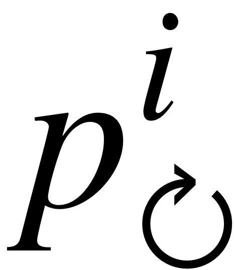
• PageRank (Coscia, 2021) assesses the relative importance of nodes based on ensembles of random walks. Originally developed to rank websites, it extends the node strength notion of importance by accounting for the influence of neighboring nodes (i.e., a node is important if it is frequently visited and connected to other frequently visited nodes). For a node v_i, the PageRank p_i is given by the recursive relation:

  $$\begin{array}{}\text{(6)}& p_i=\mathit{\alpha }\sum _{j\ne i}{\displaystyle \frac{p_j{w}_{ji}}{{\sum }_{k\ne j}{w}_{jk}}}+{\displaystyle \frac{\mathrm{1}-\mathit{\alpha }}{\left|\mathcal{V}\right|}},\end{array}$$

  where $\mathit{\alpha }\in [\mathrm{0},\mathrm{1}]$ is the damping factor (set to α=0.9, reducing teleportation relative to the common α=0.85, and $\left|\mathcal{V}\right|$ is the total number of nodes. PageRank is applied iteratively and assigns higher importance to nodes that structurally emerge as end points in the stationary distribution of the random walkers ensemble, i.e., persistent ARs that propagate through the ARTN would tend to end up at these nodes.

• Edge betweenness centrality (EBC) (Coscia, 2021; Ser-Giacomi et al., 2015c) measures the fraction of shortest paths in the network that pass through a given edge. For an edge e_ij∈ℰ, edge betweenness centrality b_ij is defined as:

  $$\begin{array}{}\text{(7)}& b_{ij}=\sum _{s\ne t\ne i\ne j}{\displaystyle \frac{{\mathit{\sigma }}_{st}\left(e_{ij}\right)}{{\mathit{\sigma }}_{st}}},\end{array}$$

  where σ_st is the total number of shortest paths between nodes v_s and v_t, and σ_st(e_ij) is the number of such paths that pass through edge e_ij. Importantly, we invert edge weights for the shortest path search to ensure that shortest paths traverse edges exhibiting the highest AR transport frequency. By doing so, “shortest path” becomes equivalent to “maximum-weight path” or “most probable path” (Ser-Giacomi et al., 2015b). EBC highlights critical conduits that connect frequently traversed regions of the network.

• Discretized IVT:
  We quantify edge- and node-wise moisture transport in the ARTN from IVT differences along individual AR trajectories. For each trajectory segment of an AR, the IVT difference between destination and origin is computed. The differences across nodes

  $$\mathrm{\Delta }{\mathrm{IVT}}_{\text{node}}\left(i\right)={\stackrel{\mathrm{‾}}{\mathrm{IVT}}}_{\text{out}}\left(i\right)-{\stackrel{\mathrm{‾}}{\mathrm{IVT}}}_{\text{in}}\left(i\right),$$

  derived from incoming/outgoing IVT values ${\stackrel{\mathrm{‾}}{\mathrm{IVT}}}_{\text{in}}\left(i\right)$/${\stackrel{\mathrm{‾}}{\mathrm{IVT}}}_{\text{out}}\left(i\right)$ are aggregated per node and express whether node i acts as a net moisture source or sink. The differences per edge

  $$\mathrm{\Delta }{\mathrm{IVT}}_{\text{edge}}(i\to j)={\mathrm{IVT}}_j-{\mathrm{IVT}}_i,$$

  with edge IVT differences IVT_i, IVT_j reflect moisture gain or loss along transport pathways. Each resulting net balance is assigned to one out of seven ordinal classes that represent the range of AR IVT gains/losses, derived from the network's global node/edge IVT difference distribution, respectively. In particular, class thresholds are determined from the empirical quantiles of the pooled IVT difference distribution across all ARs in both AR catalogs (Fig. S13). Strong losses (lowest quantile) correspond to a typical AR (mean IVT ≈ 500 $\mathrm{kg}{\mathrm{m}}^{-\mathrm{1}}{\mathrm{s}}^{-\mathrm{1}}$) losing up to 10 % of its IVT along this edge (on average), whereas strong gains (highest quantile) correspond to gaining up to 8 % of its IVT. This simple classification provides a simplified yet physically meaningful representation of IVT dynamics embedded within the ARTN topology.

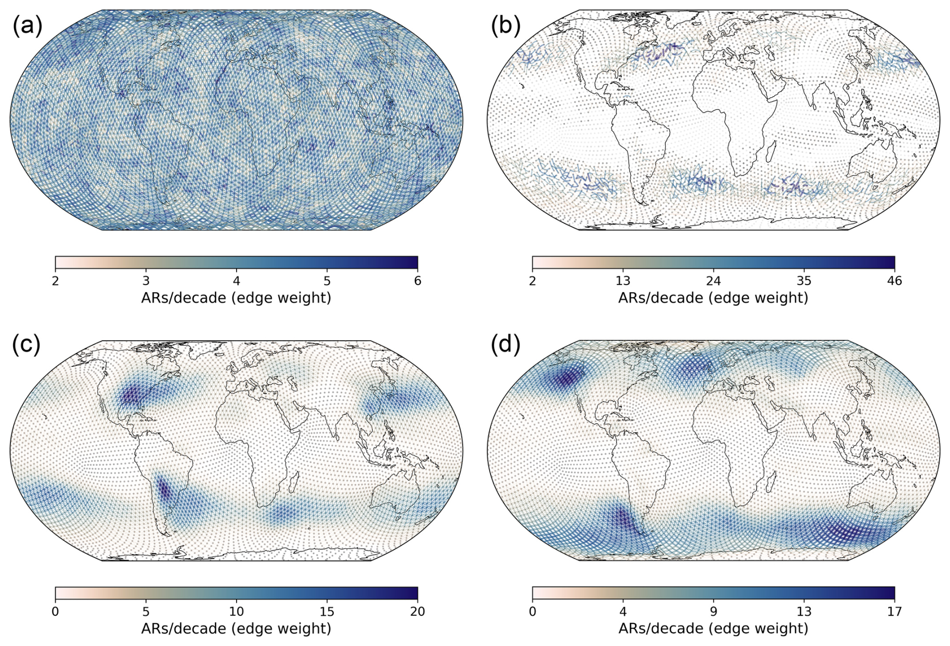
Figure 1 The four conceptually distinct types of statistical null models considered in this study. A single realization of the (a) Fully Random Walker (FRW), (b) Rewired Graph (RWG), (c) Genesis-Constrained Random Walker (GCW), and (d) Termination-Constrained Random Walker (TCW) network. The resulting networks (a) exhibit fully random connectivity, (b) conserve large-scale but randomise short-range transport patterns, (c) preserve AR genesis, and (d) preserve termination regions, respectively. Colors indicate the frequency of AR transport, represented as edge weights and expressed as ARs per decade (individually for each panel).

2.6 Community detection

We apply the Infomap algorithm to detect hierarchical communities in our directed, asymmetric, weighted transport networks (Edler et al., 2025). Infomap is a flow-based method that detects community structures based on random walks on the network. Infomap is well-known for detecting hierarchical communities across scales. In its core, it relies on the map equation:

$$\begin{array}{}\text{(8)}& L\left(M\right)=\textcolor{red}{}H\left(\mathcal{Q}\right)+\sum _i\textcolor{red}{}H\left(M^{\mathrm{i}}\right)\end{array}$$

where:

• is the total probability of exiting any module.

• $H\left(\mathcal{Q}\right)=-{\sum }_i\frac{\textcolor{red}{}}{\textcolor{red}{}}\log \frac{\textcolor{red}{}}{\textcolor{red}{}}$ is the entropy of the module exit probabilities.

• is the total probability of being inside module i, including its submodules.

• $H\left(M^{\mathrm{i}}\right)=-{\sum }_{\mathit{\alpha }\in i}\frac{p_{\mathit{\alpha }}}{\textcolor{red}{}}\log \frac{p_{\mathit{\alpha }}}{\textcolor{red}{}}$ is the entropy of the codebook for module i.

The description length of each submap Mⁱ at intermediate levels is computed analogously to the single-level formulation. Neither the number of levels nor the number of communities therein needs to be specified but emerges naturally from the random walkers' residence times within different parts of the network, rendering it a natural method to study AR transport dynamics. For a more detailed overview of the method we refer to the excellent description in Rosvall and Bergstrom (2011).

We normalize all edge weights such that their sum over the full network equals one. Isolated nodes are added to the Infomap structure explicitly to maintain a node set that completely covers the entire Earth. We consider edge directionality and omit self-loops. We filter out communities with fewer than 15 nodes to prevent them from shrinking substantially below the average synoptic-scale size of an AR. Nodes in such small communities are excluded from analyses at the corresponding and higher hierarchical levels. We apply Infomap twice: once in its standard single-level mode (Fig. 5) and once in its multilevel mode (Fig. 6) to extract a hierarchy of nested communities. In the hierarchical case, communities are recursively subdivided into sub-communities if this leads to a more efficient description of random walk flows, offering insights on how smaller AR basins are nested into larger AR basins.

To evaluate the quality of the detected communities, we compute the flow retained within a community relative to the flow exchanged with other communities:

$$\begin{array}{}\text{(9)}& \text{Flow Ratio}={\displaystyle \frac{\text{Intra-community flow}}{\text{Inter-community flow}}}\end{array}$$

where intra-community flow is the sum of flows along edges within a community, and inter-community flow is the total flow along edges connecting the community to others. High flow ratios indicate the desirable property that nodes in a community are connected considerably more strongly than to nodes in other communities.

3 Results

We construct the displayed ARTN based on tracking individual ARs across their life cycles: when an AR travels between two grid cells, we create an edge connecting those cells as nodes in the network. We sparsify the network by only considering edges exceeding a minimum transport frequency of 2 ARs per decade (see Figs. S8/S9).

ARs form global moisture transport belts through the pathways they revisit. The complex transport system that emerges from these pathways manifests as a sparse atmospheric river transport network (ARTN), revealing the planetary-scale organization of how ARs traverse the Earth's atmosphere (Fig. 2a). The global ARTN aggregates all global AR transport patterns, including four regions of high connectivity along the mid-latitude storm tracks: (i) a Northern Hemisphere (NH) western Pacific route from East Asia to the American West Coast, (ii) a North Atlantic route from eastern North America to Europe, (iii) a southwestern Pacific route towards the Chilean coastline, and (iv) a spatially extensive Southern Hemisphere (SH) route across the South Atlantic and Indian Ocean (Fig. 2a). Along these routes, edge weights are enhanced within a core region and fade out towards their boundaries.

The PIKART-1.0 catalog (Fig. S14a/b) shows densely connected regions in the (sub)tropics (e.g., close to the Caribbean low-level jet, the Amazon, the La Plata basin, the Somali low-level jet as well as tropical southeast Asia), while the tARget-4 ARTN (Fig. S14d/e) indicates strongly enhanced poleward AR moisture transport as well as cross-continental transport through North America and Eurasia. Overall, the observed mid-latitudinal main routes are more spread out in tARget-4 (Fig. S14d) than in PIKART-1.0 (Fig. S14a). This results in minor edge mismatches and notably higher edge weight differences within the core storm tracks (Fig. S15a/b, e/f). The strongest mismatches are found in the tropics where PIKART-1.0 suggests higher AR transport frequencies and in the high-latitudes where tARget-4 yields more network edges with higher weights. As intended, the consensus network (Fig. 1a) successfully enhances common transport patterns while preserving pathways that individual catalogs attest with high confidence. Edge directions in the extratropics are consistent across both catalogs, reflecting coherent advection across the storm tracks (Fig. S15).

Several other AR detection tools (ARDTs) with tracking capacities exist from which many focus mostly on the extratropics (e.g., IPART-1 (Xu et al., 2020a)) or solely cover the mid-latitudes (e.g., AR-CONNECT (Shearer et al., 2020a)). The resulting ARTNs accordingly exhibit no edges in the tropics and polar regions (Fig. S16i/j, m/n). Furthermore, they yield denser ARTNs along the mid-latitudinal storm tracks (Fig. S16c/d, g/h). Comparing all available datasets of AR trajectories collected in the ARTMIP database by means of their ARTN topologies and network metrics could further quantify these uncertainties and inform effective AR tracking strategies.

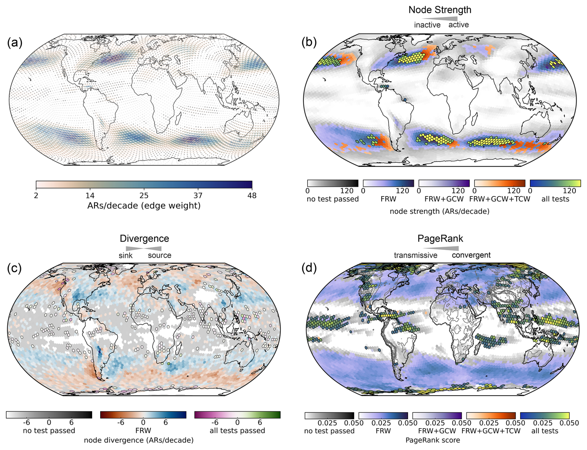
Figure 2 The global AR transport network with its sources, sinks, and structural accumulation points (1940–2023). (a) The ARTN is constructed as a consensus network from the PIKART-1.0 and tARget-4 catalogs (ϵ=2 ARs per decade). Nodes represent centroids of hexagonal grid cells and edges show AR transport frequency (ARs per decade) between grid cells. Edge directions are omitted. Colors indicate transport frequency. (b) Node strength of each node, tested against all four null models. (c) Node divergence of each node, tested against the FRW (Fully Random Walker) and the combination of all four null models. (d) PageRank score (normalized to % of total accumulated “AR walker mass”, yielding a stationary probability value) of each node (tested against all four null models). The colour maps in panel (b)–(d) indicate which set of tests was passed while still showing continuous variations of the respective network metric. Nodes that pass all tests are highlighted with a black frame.

3.1 Hubs of global atmospheric river transport

Previous research has unambiguously identified the mid-latitudinal storm tracks as the regions of highest global AR activity (Guan and Waliser, 2019). Here, ARs typically emerge from the large western ocean basins, propagate eastward and terminate along main coastlines. As a proof-of-concept, we derive node strengths (the sum of all edge weights entering or leaving a node) and test whether this pattern is recovered. Node strength reliably tracks the global regions of highest transport activity (Fig. 2b). Applying all developed null models to node strength shows that highly active nodes in the western ocean basins mark AR hotspots due to their role as AR genesis hubs (N. Atlantic, N. Pacific, S. Atlantic, S. Pacific, S. Indian Ocean), propagate eastward across hubs of strongly enhanced AR activity that pass all tests and terminate with their centroids typically located just off the coast. The core regions of the storm tracks pass all tests, suggesting AR activity here goes beyond AR genesis, termination and large-scale transport. Superimposed on the west-to-east gradient, a northward-propagation pattern tracks AR transport towards the poles (Fig. 2b).

Node divergence – the difference of incoming and outgoing edges for a given node – clearly confirms this large-scale transport pattern (Fig. 2c). Negative (positive) node divergence suggests a node acts predominately as an AR sink (source). Extending past familiar patterns, node divergence captures more complex genesis and termination hubs. In some regions with large continental lakes or seas (eastern Eurasia, eastern North America), intense moisture recycling (the Amazon basin, the La Plata basin) or strong coastal moisture gradients (North Africa/Mediterranean), nodes with significantly high negative and high positive divergence coexist in close spatial proximity, implying more intricate AR transport in and out of these regions.

If common AR pathways are traced repeatedly through the network, which nodes emerge as their most frequent long-term destinations (Fig. 2c)? By identifying the stationary distribution of an ensemble of random walkers that follow the ARTN, PageRank highlights regions that AR pathways repeatedly converge upon, effectively revealing the network’s structural “attractors”/topological sinks (beyond the basic notion of “high AR activity” provided by node strength). Most nodes exhibit higher PageRank scores than expected from random dynamics (blue pixels), with some of the highest values at known AR landfall hotspots like western North America. The Arctic and Antarctica show highly significant scores, stressing that intense, persistent ARs can reach these highly susceptible regions from many parts of the network with potentially severe hazards and impacts (Maclennan et al., 2025; Wang et al., 2024).

Elevated PageRank scores also emerge along major orographic barriers (southwestern Himalaya, southern Andes, northern Rocky Mountains), across monsoon regions such as Southeast Asia, and within key moisture recycling hubs including the Amazon basin and eastern boreal forests. Several of these regions also show significantly high (cycle) clustering coefficients (Fig. S17, e.g. the Amazon basin and the Himalaya), suggesting spatially confined, recurrent AR transport that translates to strongly interconnected regions in the ARTN. This is compatible with PageRank scores as a proxy for nodes at which ARs tend to reside for longer time periods, partly within isolated network components. The shifts of the identified AR hubs when using AR head coordinates are shown in Fig. S12.

In tropical monsoon areas, AR detection remains uncertain and formation mechanisms poorly understood. The high PageRank scores here may partially reflect spurious AR detection in the PIKART-1.0 catalog (especially along the tropical Pacific) but could also support the idea of tropical ARs as a “continuum of extratropical and monsoonal moisture plumes” (Park and Son, 2024) with high potential to generate extreme precipitation (Lyngwa et al., 2025). Future studies could scrutinize AR dynamics in these regions to resolve this uncertainty.

3.2 Tracking AR Vapor Transport Changes

Where do ARs tend to strengthen or weaken their vapor transport? We derive net IVT changes across each node in the ARTN (Fig. 3a). AR intensification is not limited to ocean basins: Eastern North America, the La Plata basin, eastern Asia as well as parts of Australia can be clearly identified with continental nodes of enhanced IVT intensification. On the other hand, eastern Eurasia and the Amazon basin show less clear tendencies of IVT change and IVT into North Africa is overall balanced. Some nodes across which ARs clearly tend to intensify their vapor transport align strikingly well with well-known low-level jets (LLJs), e.g., the Great Plains LLJ, the Caribbean LLJ, and the southward nocturnal LLJ extension of the South American LLJ (Gimeno et al., 2016). The Western Hemisphere Warm Pool represents one of the main NH evaporative regions and has been previously identified as a global hub of AR moisture uptake (Algarra et al., 2020), but Fig. 3a additionally reveals that the LLJs can be distinguished from a background of overall high moisture uptake.

Another region of markedly enhanced IVT gains emerges at the southern tip of South Africa, likely driven by moisture input from South America that drives cold-season ARs over western South Africa (Ramos et al., 2019). The most prominent IVT depletion hubs (western North America, southwestern South America, the British Isles) align well with AR transport sinks (Fig. 2b/c) and correspond to regions with a strong dynamic IVT component, where high IVT is closely tied to heavy precipitation (Gimeno et al., 2016).

If individual ARs pass across multiple nodes that tend to intensify IVT, this could imply higher IVT at landfall (and potentially stronger AR hazards and impacts). We test the presence of such correlations and the implied degree of predictability by examining the relationship between the mean IVT classifier over each AR's life cycle sequence and its IVT at first landfall. ARs in the PIKART-1.0 (tARget-4) catalog exhibit a significant Pearson correlation of 0.39 (p<0.01) (0.22 (p<0.01)), respectively (Fig. S18). Given the substantial complexities involved in predicting the intensity of an AR at landfall, this significant relationship is encouraging.

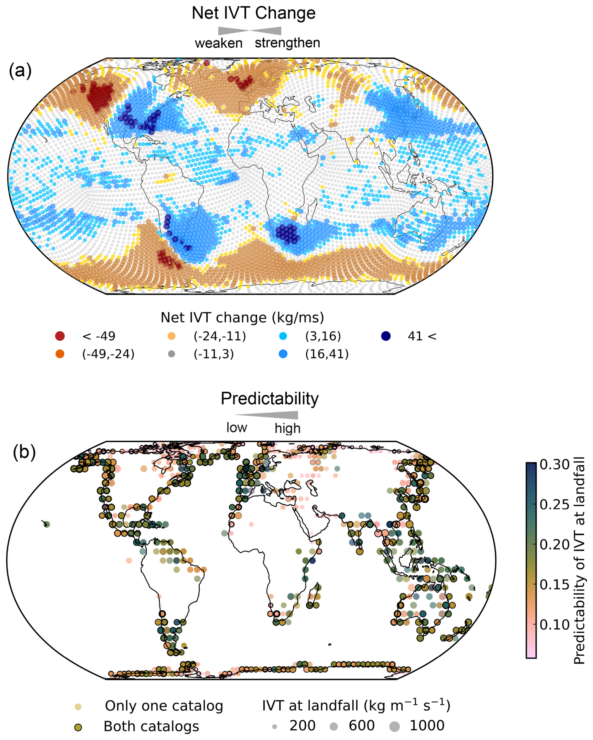
Figure 3 Net changes of IVT across nodes and IVT predictability scores at all recorded AR landfall locations. (a) Net IVT changes, i.e., along which nodes ARs tend to intensify or weaken their IVT. IVT changes of individual ARs are compared to the global change distribution and classified into seven discrete classes based on the distribution's quantiles. (b) Predictability score, derived from the residuals of a robust linear Huber-regression of IVT changes against IVT at landfall (averaged over both catalogs and each landfall location). The maximum predictability score is normalised to the average overall correlation between both variables. Marker size denotes IVT at landfall. Landfall locations recorded in both AR catalogs are highlighted with a black frame.

We unravel where the identified link is most strongly expressed by performing a robust linear Huber regression between both variables and extracting the residuals of the regression. Each residual is divided by the respective overall correlation value noted above so that the highest predictability is scaled by the overall correlation (Fig. 3b, averaged over all AR trajectories and both catalogs at each landfall location). Coastal mid-latitudinal regions that are frequently exposed to high intensity ARs (e.g., California (marker size)) exhibit relatively high predictability scores. Predicting landfall IVT in polar regions and in the (sub)tropics appears more challenging. The PIKART catalog allows ARs to make landfall at non-coastal grid cells where predictability is overall lower. These results, that are based on a simple linear model, point towards the predictive potential of the developed approach, which could be exploited in future studies.

3.3 A highway system of atmospheric river pathways

Edges in the ARTN encode crucial information about prominent AR pathways. As the emergent “roads” of global AR transport, they hold significant potential for improving forecasts of AR trajectories. We investigate where the most vital edges are located by computing the edge betweenness centrality (EBC) of each edge, i.e., which edges act as critical conduits of AR transport. Edges with low AR frequency are considered more “costly”. Thus, EBC is expected to carve out a set of edges that many ARs must cross. An edge with high EBC connects many pairs of nodes along their most likely AR routes. If that connection was disrupted, many paths that potentially link important but spatially distant regions would be blocked. We find a system of cohesive “AR highways”, along which ARs orient their flow, show clear tendencies of IVT gains/losses and which are modulated by large-scale atmospheric circulation (Fig. 4).

The observed AR highways form a near-continuous belt encircling the globe in both hemispheres. All major branches are statistically significant (95 %-confidence level, Fig. S19). The NH branch of the global AR highway pierces through northwestern North America with high EBC and spans across the North America continent, primarily supported by strong EBC edges in the tARget-4 network (Fig. 4a). Both catalogs also reveal a less prominent but notable branch towards California. The highway then veers towards northwestern Europe and splits into smaller branches reaching northern Africa, central Europe, the Arctic, and the Mediterranean. The main branch passes through the British Isles and northern Europe, continues across eastern Eurasia, and ultimately arrives in East Asia, where it merges with a fork-shaped (sub)tropical branch (identified only in the PIKART-1.0 network). After merging, it forms the well-known trans-Pacific AR pathway to the western United States. PIKART-1.0 also detects an AR highway across the central Pacific, linking Southeast Asia to the Caribbean. In the SH, both catalogs consistently identify a major AR highway extending from eastern South America across the Southern Ocean. Weaker offshoots connect this main SH highway to interior South America, South Africa, and South Australia. Some of these are not statistically significant (95 %-confidence level, Fig. S19), likely owing to the fact that they act as “one-way roads”. They can, however, still be considered important entry points from major AR genesis regions and some of them (e.g., the one exiting interior South America) exhibit high AR frequency. EBC reacts more sensitively to changes in the network threshold or spatial resolution than, e.g., node strength (Figs. S7/S9).

The network of high-EBC edges can be regarded as a planetary-scale transport belt that guides ARs through the underlying ARTN. In this context, guiding refers to the dynamical constraint imposed by large-scale upper-tropospheric circulation patterns on the preferred pathways of AR propagation. Specifically, the location and spatial extent of this high-EBC backbone align well with the spatial structure associated with the circumglobal teleconnection pattern, whose dynamical expression is a quasi-stationary Rossby wave train in the upper troposphere (Ding and Wang, 2005). Generally, low-frequency upper-level atmospheric circulation modulates Rossby wave-breaking events which, in turn, control low-level weather systems such as (anti)cyclones (Tamarin-Brodsky and Harnik, 2024) and ARs (Ryoo et al., 2013). Wave breaking events along the circumglobal teleconnection pattern amplify upper-level anticyclonic anomalies and create persistent jet streaks that steer and intensify AR pathways along preferred longitudes (Zavadoff and Kirtman, 2020). The resulting waveguide enhances the zonal coherence and longitudinal continuity of AR transport, supporting the emergence of a contiguous high-EBC AR backbone. This mechanism elucidates how ARs are efficiently navigating through the troposphere, e.g., from the North Atlantic across Eurasia and the North Pacific back to North America during boreal winter. While some previous work has conducted regional analyses of how Rossby wave breaking along the mid-latitudinal jets control AR propagation (Hu et al., 2017), our results provide the first evidence of a contiguous AR transport backbone along which these processes organize globally.

Along all AR highways, we derive net IVT gains and losses that can be induced by changes in moisture or winds (Fig. 4b). As expected, coastlines and mountainous regions deplete ARs of their IVT, likely through orographic precipitation (e.g., western North America, the British Isles, and Chile). Over the western ocean basins identified as AR sources (Fig. 1b), cyclogenesis plays a major role and ARs tend to fuel up their IVT (either through enhanced evaporation or strengthened winds or a combination of both) (Gimeno et al., 2016). Beyond oceanic sources, several continental regions stand out as key conduits along which ARs gain IVT (eastern North America, Central and East Asia) and some oceanic regions are associated with IVT losses (the North Atlantic branch towards Europe, segments of the southern Ocean branch).

Finally, the SH branch of the AR highways follows a wave-like pattern of IVT gain and loss (Fig. 4b, also prominent in Fig. 3a), reminiscent of the zonal wave-3 pattern – a dominant SH circulation mode that produces alternating ridges and troughs in geopotential height (Goyal et al., 2021). In geostrophically balanced flow, horizontal pressure gradients primarily organize the large-scale waveguide along which ARs propagate, while ageostrophic circulations associated with ridges and troughs induce convergence and ascent, promoting moisture conversion to precipitation (Dacre and Clark, 2025). These processes modulate AR pathways and moisture content along preferred longitudes, offering a physically consistent explanation for the observed pattern.

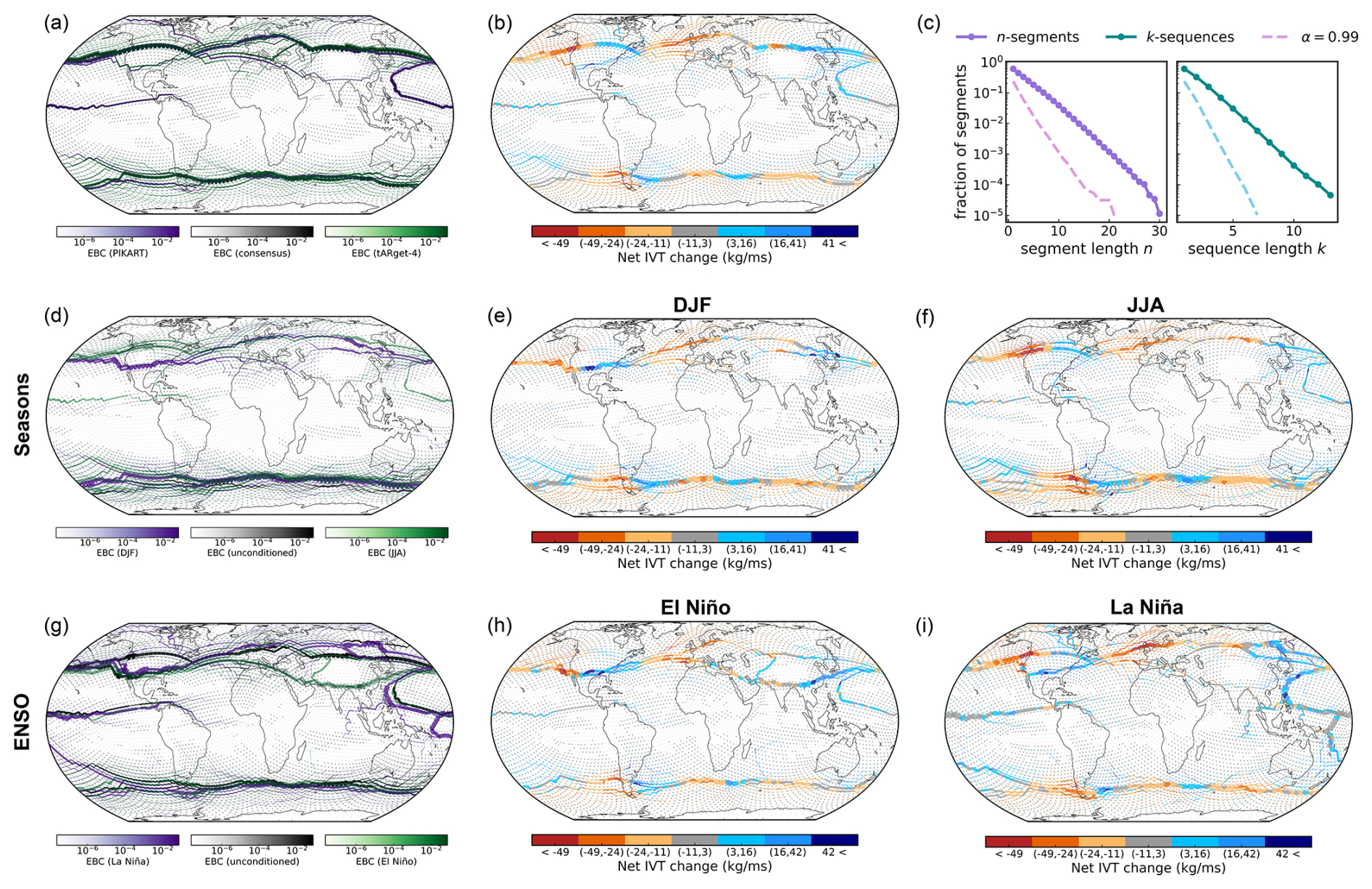
Figure 4 Network of global “AR highways”, redirected by climate oscillations. Edge widths are scaled logarithmically according to their EBC (edge betweenness centrality) values. Edge colours distinguish between the two AR catalogs in (a) and between opposing phases of the respective climate oscillation in (d)/(g). Edge colours in (b), (e)/(f), (h)/(i) denote whether ARs tend to lose or gain IVT along a given edge. (a)/(b) Unconditioned AR highways (ϵ=2 ARs per decade), reconstructed from the tARget-4 (green) versus PIKART-1.0 (purple) catalog, with consensus network (grey) for reference. (c) Fraction of n-segments and k-sequences of AR transport along any AR highway, compared to 200 random null model realizations (99 %-significance level, dashed lines). Each segment or step in a sequence corresponds to 6 h spend along an AR highway. (d)–(f) Seasonal modulations of AR highways: DJF (green) versus JJA (purple), with non-conditioned network (grey) for reference. (g)–(i) Modulations of AR highways by ENSO phase: (g) El Niño (green) versus La Niña (purple), with neutral state (grey) for reference.

The notion of “AR highways” prompts the question of how closely individual ARs actually follow them. We classify ARs into three groups based on how closely their trajectories align with major AR highways: Conformists, Straddlers, and Strays (examples in Fig. S20a–c). Conformists follow highways most rigidly, while Straddlers deviate more often and Strays exhibit marked anomalies, sometimes venturing far off the main branches. Statistical tests confirm that Strays differ significantly in intensity (but not in lifetime), tending to transport more moisture, while Straddlers exhibit enhanced lifetimes (Fig. S20d/e).

To further quantify the tendency of ARs to propagate along the discovered highways, we compute (i) the fraction of AR trajectories (≥24 h) that traverse at least n highway segments during their lifetime, and (ii) the fraction of k-sequences, i.e., trajectories that follow a highway (10 % of edges with highest EBC) for at least k consecutive steps (Fig. 4c). Both fractions substantially exceed random expectations (99 % significance from 200 random-walk ensembles with the same number and lengths as in the PIKART catalog). Hence, highways increase the predictability of AR transport: ARs are drawn toward high-EBC edges, and once aligned, tend to remain on them.

3.4 AR highways are modulated by climate oscillations

While AR seasonality has been extensively studied in North America and Western Europe (Rutz et al., 2019), research in other regions is only emerging (Ye et al., 2020; Viale et al., 2018; Pan and Lu, 2020). We delineate AR highways during December-January-February (DJF, boreal winter) from those in June–July–August (JJA, boreal summer) by conditioning the underlying ARTNs (Fig. 4d–f, conditioned ARTNs shown in Fig. S21). The band of highest AR activity towards western North America closely tracks the mean position of the eddy-driven jet across seasons, with a gradual migration from its most poleward position in JJA to its most equatorward position in DJF (Rutz et al., 2019). AR transport patterns into Europe are more complex, but overall, previous studies showed that weakened storm tracks guide less ARs towards the European West coast in JJA than in DJF when some ARDTs record peak AR frequencies (Rutz et al., 2019). We identify an overall similar backbone of high EBC edges in both seasons with a slightly less pronounced branch towards southern Europe during JJA (Fig. 4d).

In the SH, seasonal AR highways are not as sharply distinguishable but organise along a more continuous band of high EBC edges. During austral winter (JJA), ARs reach further north along the Chilean coastline and deplete significant amounts of IVT. Across the Southern Ocean, the identified AR highways do not differ considerably between both seasons apart from stronger branching towards southern Australia in JJA.

To showcase that the AR highways revealed here are modulated by climate teleconnections, we condition the ARTN on El Niño/La Niña episodes of the El Niño Southern Oscillation (ENSO) (Fig. 4g–i, conditioned ARTNs shown in Fig. S21). We classify El Niño (La Niña) episodes by detecting episodes for which the Oceanic Niño index exceeds (falls below) a value of 0.5 (−0.5) for at least five consecutive 3-month averages (Fig. S22). Previous studies found conflicting results on the role ENSO plays in reshaping AR pathways towards western North America, with some finding a significant equatorward (poleward) shift during El Niño (La Niña) episodes (Payne and Magnusdottir, 2014) while others found other teleconnections to be more relevant, e.g., the Madden-Julian Oscillation or the Pacific-Japan teleconnection (Zhang and Villarini, 2018; Guan and Waliser, 2015). We find that – at hemispheric and planetary scale – ENSO does substantially reshape AR highways. Towards northwestern North America, La Niña generates a distinctive branch (Fig. 4g). Across the North Atlantic, La Niña continues to direct ARs further poleward than El Niño with various smaller branches reaching into the Arctic. Across interior Europe, ARs tend to stay higher north, consistent with a poleward displaced jet. Conversely, El Niño channels AR highways further south with a prominent branch that crosses over the Mediterranean towards the Middle East and northern India before it ascends again towards Japan. In the (sub)tropics, La Niña generates more prominent AR highways that originate in the central-eastern Pacific and exhibit both an ascending branch towards western North America and a descending branch towards South America (similar to the findings in Guan and Waliser, 2015). Across the Southern Ocean, no major differences between the dominant branches can be identified. In most regions, IVT gains and losses do not differ substantially along La Niña and El Niño AR highways (Fig. 4h/i). However, we do find stronger tendencies of ARs to weaken their IVT during La Niña at some of the main AR landfall hotspots, including western North America, Europe, and Chile. Overall, the regions where ARs exhibit the strongest tendencies of IVT change are relatively stable across the studied seasons and ENSO regimes with the most considerable deviations in the (sub)tropics (Fig. S23).

3.5 Across which basins do ARs organize?

Most AR studies have a regional focus. Hence, our understanding of global AR basins – regions where individual AR trajectories tend to originate, evolve, and dissipate within the same broader area and AR activity is tightly interconnected – remains incomplete. Previous work has applied clustering algorithms to AR conditions (rather than trajectories) within a few confined regions (Ryoo et al., 2015; Zhang and Villarini, 2018; Pan et al., 2024). These regional, Eulerian methods overlook the connectivity of individual AR trajectories and can introduce spurious boundary effects by cutting across AR tracks that enter or exit the region.

Here, we instead detect AR basins as communities in the global ARTN from the more natural Lagrangian perspective using the Infomap algorithm (Rosvall and Bergstrom, 2011). Physically, AR communities can be understood as enclosed geographical regions whose boundaries are determined by persistent steering flows, topography, coastal moisture gradients and thermodynamic limits on AR life cycles (depending on the rates of evaporation and precipitation over an AR's life cycle). We evaluate the performance and stability of the real AR communities against those obtained from the developed null models (Figs. S24–S26). Given the stochastic nature of Infomap, we assess its robustness by running the single-level mode for 100 different random seeds. We evaluate its overall stability through Adjusted Mutual Information and Adjusted Rand Scores and compare it to 95 %-confidence levels obtained from the different null models. For each node, we furthermore quantify heterogeneity/label inconsistency as one minus the average Jaccard similarity between the sets of nodes it is grouped with across runs, capturing the consistency of its community assignments (Figs. S24/S25). We derive a setwise consensus partition by assigning each node to the most frequently co-occurring community set across all seeds. This strongly fragments community assignments for less stable communities (Fig. S24c). More sophisticated consensus clustering approaches would likely lead to a more sound consensus partition but are computationally intense. Instead, we consider the most central partition as the one whose community structure exhibits the lowest overall node-wise heterogeneity, weighted by community size (Figs. 5a, S24a). AR basins are not fully independent. For any pair of neighbouring basins, a certain degree of inter-basin traffic can be expected.

We uncover that global AR transport is organized across dozens of basins of various sizes and shapes (Fig. 5a). In the NH, the trans-Pacific and trans-Atlantic basins are most well-separated and stable (marked by high flow ratios and strong partition stability, see Fig. S24b–d). They closely match the stability of the GCW/TCW null models (Fig. S26), attesting high confidence: by definition, the GCW/TCW null models achieve high stability through their constrained AR genesis/termination regions which form strong communities in an otherwise random network.

The trans-Pacific basin splits near 175° E, suggesting that some ARs terminate early en route to western North America (in agreement with Pan et al., 2024). The northwest American coastline is intersected by five AR basins: two small basins over California and the Pacific Northwest (both likely enhanced during DJF, see Fig. 4e), a northern extension into Canada and two high-latitude basins that intersect with Alaska. The lower-latitude basins align well with previous classifications (Zhang and Villarini, 2018). The northern extension into Canada aligns with the entry point of inland-penetrating ARs responsible for triggering extreme precipitation over the continental interior (Vallejo-Bernal et al., 2023). Over interior North America, community boundaries track topography, particularly the Rocky Mountains and the Appalachians.

Towards Europe, a large AR basin is bordered by four basins along the western coast: two southern basins via Iberia and the Mediterranean, a central basin covering large stretches of coastal and interior central Europe, and a northern branch reaching across Arctic coastlines. Interior Europe hosts additional AR basins, some of which transition towards Central Asia, indicating that various ARs penetrate far into the Eurasian continent. Similar to North America, mountainous regions such as the Ural Mountains and the Alps manifest as AR basin boundaries. AR communities over the Middle East and Northern Africa are identified less stably (Fig. S24b–d), indicating a stronger degree of fragmentation of AR tracks across these regions. While the larger hemispheric AR routes are well established, many of these basins have not previously been systematically identified as the strongly interconnected systems revealed here.

In the (sub)tropics, we find that few AR basins exceed 15 grid cells, highlighting fragmented AR motion. Notable exceptions include zonal basins over the Central Pacific and an isolated Caribbean basin. Conversely, SH AR basins are spatially extensive and more elongated. We identify the most robust and well-separated communities within a South Pacific basin that is directed towards South America and two basins over the Southern Ocean (Fig. S24b–d). The GCW replicates these robust basins, albeit more spatially confined around AR genesis hotspots (Fig. S25d–f). However, higher uncertainty remains over regions such as southern South America, Oceania, and Antarctica (Fig. S24b/d).

AR lifecycle characteristics differ considerably between the identified basins (Fig. S27 and Table S1). Mid-latitudinal oceanic basins (e.g., basin #7 and #3 in the NH or basin #1 and #2 in the SH) host intense, long ARs (IVT ≈490–550 kg m⁻¹ s⁻¹, length ≈3700–4000 km) with relatively long residence times (40–60 h; partly confounded by their large spatial extent). Baja California (basin #40, 49.7 %), the southern Iberian Peninsula (basin #34, 44.8 %), and the Mediterranean coast (basin #33, 41.5 %) exhibit some of the highest AR inland penetration frequencies. ARs also appear to penetrate well into Alaska (basin #38, 35.9 %) and northern Scandinavia (basin #26, 35.3 %). Basin #11 (eastern China and Japan) receives relatively short but very intense ARs (IVT = 584 kg m⁻¹ s⁻¹, residence ≈27 h). Basin #8 (Central Asia) is entirely land-locked (97.5 % land) with relatively high residence times (≈31 h) and moderate IVT (289 kg m⁻¹ s⁻¹), indicating potential moisture recycling. While not exhaustive, this analysis showcases how the identified basins provide a coherent spatial framework for stratifying AR transport patterns, exposing regional contrasts in moisture transport, persistence, and land interactions that hemispheric or storm-track-based views would obscure.

Finally, the identified AR basins are reorganized seasonally with pronounced hemispheric asymmetries (Fig. S27). The North Pacific and North Atlantic basins extend their reach into their respective continental interior during boreal winter and some NH basins migrate poleward in boreal summer (Fig. S28a/c). In contrast, SH basins preserve their zonal continuity year-round, reflecting the persistent austral westerlies. A more intricate cluster of small Mediterranean/Middle Eastern basins emerges during SON and MAM (Fig. S28b/d), in line with a previous study that identified MAM as the dominant season for intense ARs over the Middle East (Esfandiari and Rezaei, 2022).

3.6 Net gains and losses of atmospheric vapor transport

To trace moisture pathways, we construct upstream networks by tracking ARs backward from target basins (Fig. 5b/c). For instance, some ARs strengthen their IVT over western Canada, possibly fueled by the respective LLJ or the Great Lakes (Fig. 5b, top panel). A population of ARs that traverses Hudson Bay or western Greenland originates from the trans-Pacific branch, losing significant amounts of moisture on their passage across North America (Fig. 5b, middle panel). ARs that penetrate into continental Europe across the Atlantic branch tend to start reducing their IVT once their centroid has crossed ≈ 35 ° W or keep gaining IVT along a more southerly route across northern Africa/the Mediterranean (Fig. 5b, bottom panel). IVT losses could initially be induced by ascent in an extratropical cyclone warm conveyor belt or a reduction of zonal winds, followed by orographic uplift.

In the SH, a spatially extensive Southern Ocean AR basin is fed by three distinct AR populations (Fig. 5c, top panel): ARs that surpass Chile with significant IVT losses, ARs that originate from interior South America over the La Plata basin and ARs originating from South Africa. Southern Australia draws ARs with IVT gains from a northerly route and with more IVT losses from a southerly route (Fig. 5c, center panel). ARs that may make landfall over eastern Antarctica are strongly diverted from their zonal movement, incurring large IVT losses (Fig. 5c, bottom panel).

With these examples, we clearly demonstrate how the ARTN not only delineates previously unrecognized basins of interconnected AR transport but also characterizes water vapor flows along the network. The ARTN framework thus complements computationally intense parcel-tracking approaches by offering a lightweight yet physically meaningful view into global moisture transport.

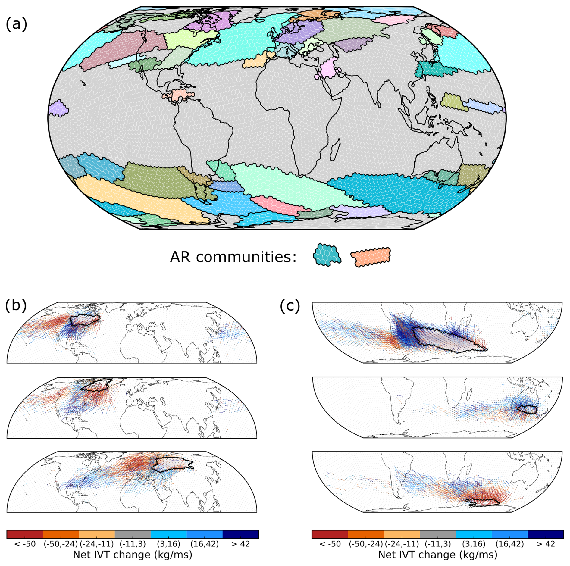
Figure 5 Global AR basins and AR moisture transport into these basins. (a) AR basins are identified as network communities using the (non-hierarchical) Infomap algorithm. Infomap is run 100 times with distinct random seeds and only the most central partition is shown. Communities with less than 15 grid cells are discarded (grey). (b)/(c) Upstream networks into three exemplary AR basins (black contours) for the NH/SH respectively. Edge colours denote whether ARs tend to lose or gain IVT along a given edge. Upstream networks are constructed “backwards” from all AR trajectories that pass through the specified basin, using only the segments leading up to their last encounter with the basin.

3.7 The hierarchical organization of atmospheric river transport

According to the prevailing paradigm, there are five main basins of global AR transport: the North Pacific, North Atlantic, South Indian Ocean, South Pacific, and South Atlantic, each serving as a major corridor for long-range moisture delivery (Park et al., 2023). Figure 5 suggests the existence of a significantly higher number of AR (sub-)basins. We investigate how these are embedded within larger basins using hierarchical Infomap community detection (Fig. 6). At the 0th level, the algorithm simply distinguishes both hemispheres (assigning the tropics to the NH, not shown). At the first level, the (sub)tropics are separated from both extratropical hemispheres (Fig. 6a). With every additional level, these large-scale communities are broken down into more fine-grained communities. Their intra- and inter-community flow (i.e., AR transport within and between communities) is shown in Fig. 5e–h and the hierarchical branching is visualized through a Sankey diagram (Fig. 6i).

At level-2, the NH AR community fragments into an Atlantic and a Pacific domain. Some tropical communities disappear as they are fragmented into sub-communities that are smaller than 15 grid cells (grey). The SH remains stable, underscoring its strong internal connectivity. The community flow is still mostly concentrated as internal flow in the two extratropical hemispheres, similar to level-1 (Fig. 6f).

Only at level-3, the flow homogenizes more equally across the globe (Fig. 6g) as communities become even more fine-grained, especially in the NH (Fig. 6c). In contrast, the SH only breaks down into less, larger communities. This asymmetry likely arises from how the hierarchical Infomap algorithm naturally splits communities in a physically meaningful way: communities are split only if doing so significantly reduces the map equation, i.e., if sub-communities offer a better compression of random walk dynamics. In the SH, AR pathways tend to follow long, coherent, and relatively uninterrupted tracks across the Southern Ocean (Fig. 6). These transport patterns translate to high internal connectivity (indicated by high internal flow, Fig. 6g) and less strongly defined substructures. Conversely, the NH exhibits more frequent AR branching and termination due to larger continental landmasses which entail numerous orographic barriers as well as thermal gradients at coasts, which in turn promotes more frequent and meaningful community subdivisions at higher levels.

At the final hierarchical level, the SH breaks up into various communities (Fig. 6d). A few of these align well with the AR basins identified in Fig. 5a. For instance, the large-scale AR basin directed towards the Chilean coast is sub-divided into multiple sub-basins, including a southern and two northern basins in Fig. 6d with strong inter-community flow. While AR flow has strongly homogenized (i.e., no single community contains the large majority of AR tracks, Fig. 6h), the most dominant communities are still the ones in the Southern Ocean (e.g., the purple and the olive basin). These two communities contain some of the globally most active AR hubs (Fig. 2b). In the NH, fragmentation has rendered many communities smaller than the synoptic-scale whereby the remaining ones form a continuous conduit that aligns with the AR highway (Fig. 4), underscoring the robustness of the main moisture transport route.

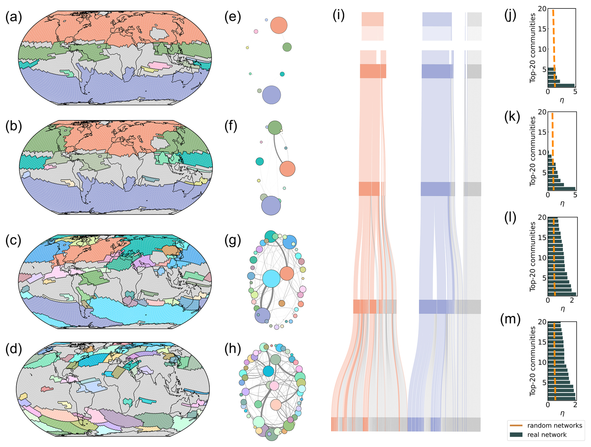
Figure 6 The hierarchical organization of AR basins as identified through Infomap community detection. Communities are arranged hierarchically from top to bottom across each column. Panels (a)–(d) show the communities from level-1 to level-4 (discarding level-0). Small communities (<15 grid cells) are absorbed into the grey background. Panels (e)–(h) display intra- and inter-community flows in a network representation where each node represents a community at the given level. Node size scales with total flow, edge width scales with inter-community flow. (i) Sankey diagram to visualize hierarchical branching of communities into smaller and smaller sub-communities. Each vertical box represents a separate community, colored by its parent community at level-0 (indicated at the top with gap below). Each connection represents how a community is split into sub-communities, with grey boxes/connections denoting discarded small communities. Panels (j)–(m) evaluate the quality of the top-20 highest flow communities at each level in terms of their flow ratio η, i.e., the ratio from intra- to inter-community flows. These are compared to the 95 %-quantile from realizations of the FRW network model.

Figure 6j–m show that, at every hierarchical level, most of the top-20 communities (by how much AR transport is contained) are significantly better separated than expected from the FRW model (95 % confidence). Only some smaller communities fall below this threshold. The discrepancies between Figs. 5 and 6 likely reflect differences in flow magnitude: many small communities in Fig. 6 lie within the range expected at random, even though the median flow ratio exceeds the 95 % quantile (Fig. S24). Thus, some smaller AR basins may be less strongly connected than the main global ones. By contrast, larger, high-flow basins – such as southern California, western Greenland, the Middle East, southern Australia, and western Antarctica – emerge as robust, understudied regions warranting further attention.

4 Discussion and conclusions

We demonstrated that Atmospheric River (AR) pathways form a distinctive, interconnected global transport network. While most prior work has studied ARs regionally and from an Eulerian hazard perspective, our network framework reveals their organization within a dynamic, planet-wide moisture system shaped by atmospheric circulation. Here, we introduced the ARTN framework and showed that it offers a versatile analysis tool. We demonstrated its potential by identifying global AR transport hubs, highways, and basins, shedding light on the structure and connectivity of AR transport on a global scale. Hubs transmit or accumulate exceptional numbers of ARs, highways act as critical conduits between them, and basins form hierarchically nested regions of enhanced connectivity. Overall, these network measures quantify topological properties of the developed ARTN rather than independent, previously unknown dynamical mechanisms. However, the ARTN unifies otherwise disparate regional phenomena into a single, quantitative representation and may help to better understand the underlying atmospheric transport mechanisms.

ARs typically originate from one of five major genesis hubs (Figs. 2/3) from which they follow a backbone of edges with high betweenness, the network of AR highways (Fig. 4). Beyond mere AR activity along the storm tracks, we reveal vapor transport hubs which offer novel insights on where ARs gain, recycle or deplete substantial amounts of their moisture (e.g., Central Asia and South Africa). While the mid-latitudinal storm tracks host the hubs of highest AR activity, we stress that the ARTN structurally directs persistent ARs towards the highly susceptible polar regions where they can cause a complex range of extremes, including surface melting events and extreme snowfall. The locations of the revealed global AR highways that guide global AR propagation vary with the seasons and respond to basic climate modes, such as ENSO. Knowledge of their positions and response times may offer a useful basis for improved forecasts of AR trajectories. The lack of cohesive source/sink regions and distinctive highways in the tropics (Figs. 2b, 3) likely reflects the different meteorological nature of (sub)tropical ARs, which are tied to low-level jets or monsoons rather than cyclogenesis or warm conveyor belts (Gimeno et al., 2020). Their heterogeneous pathways warrant closer investigation of the (sub)tropical component of the global ARTN.

Previous research suggested five major AR basins – the North Pacific, North Atlantic, South Indian Ocean, South Pacific, and South Atlantic (Park et al., 2023). We uncover a rich substructure of interconnected AR sub-basins (Fig. 5). Their high internal connectivity reflects physical constraints on AR dynamics. Their hierarchical structure underscores the multiscale nature of ARs as discrete synoptic-scale features embedded within larger flow regimes (Fig. 6), a structural property of AR transport only few frameworks so far have captured effectively (Park et al., 2023). Western Greenland, the Middle East, southern Australia, and western Antarctica emerge as noteworthy basins warranting further attention. AR basins are particularly fragmented in the NH due to orographic and land–sea contrasts. If, as argued, “not all ARs are created equal” (Zhang and Villarini, 2018), the identified basins could provide a foundation to better understand differences in AR dynamics. Future research should exploit the high internal connectivity of these basins for AR forecasting and study their structural changes over time.

Our approach complements more traditional Lagrangian and Eulerian methods (Stohl and James, 2004; Tuinenburg and Staal, 2020; Gimeno et al., 2020) by providing a scalable, data-driven, and mechanistically grounded framework for studying moisture transport. It enables comparison between AR catalogs and evaluation of model performance. Unlike correlation-based climate networks, which risk spurious links (Haas et al., 2023), our transport definition retains physical interpretability and can be meaningfully combined with graph diffusion methods. Looking forward, ARTNs could be embedded in multilayer network architectures to link AR transport with other components of the high-dimensional Earth system (e.g., the Ocean and land surface) and track their cascading hazards (Miralles et al., 2024). The ARTN could be physically substantiated by linking edge weights to physical water flows within a constrained water balance (De Petrillo et al., 2025). Finally, akin to how transport networks revolutionized traffic prediction (Jiang and Luo, 2022), network-based modeling and graph neural networks offer a pathway toward predictive tools for AR dynamics by learning the underlying structural rules of their propagation. The first steps taken here to demonstrate this predictability – inferring landfall IVT from edge sequences and quantifying how ARs follow the discovered highway system – revealed a moderate but promising degree of predictability.

Altogether, our work lays the foundation for future studies on global Lagrangian analyses of AR trajectories, potentially improving AR predictability, and scrutinizing AR-related risks under climate change. For studying how synoptic meteorology connects to planetary-scale climate dynamics, we advocate shifting the prevailing AR paradigm from Eulerian, localized events toward a Lagrangian perspective that follows AR trajectories and captures their transitions and dynamics. The global AR network offers a framework to better understand how AR pathways may shift, intensify, or reorganise in a warming world. Moreover, it opens the door for applying similar network-based methods to AR-induced heat or aerosol transport, as well as other weather features (e.g., fronts or cyclones) (Prein et al., 2023). This could enable a broader rethinking of global hydrological connectivity.