Attribution of changes in winds over the Southern Ocean from 1950 to 2100

Strong near-surface westerly winds drive the Southern Ocean circulation and play a key role in setting regional and global climate. In the latter half of the 20th century, depletion of stratospheric ozone over Antarctica has caused these winds to accelerate and move polewards, particularly in austral summer. However, the future evolution of these winds remains uncertain. We use reanalysis data and the UK Earth System Model (UKESM1), with full atmospheric chemistry, to assess the drivers of winds over the recent past and coming century. We first characterize the wind mean state, distribution, and trends over 1980–2019 in the most commonly used atmospheric reanalyses (ERA5, JRA3Q, and MERRA2) to gain insight into observed wind behaviour in the past. We show that while the representation of the mean wind is similar among reanalyses, MERRA2 shows stronger wind acceleration trends that persist year-round, while JRA3Q and ERA5 show weaker acceleration, primarily in austral summer. Using an observational Southern Annular Mode (SAM) index, we show that the weaker, summer-focused trends of JRA3Q and ERA5 are likely more realistic. UKESM1 represents historical trends in winds accurately compared to ERA5 and is within the range of other CMIP6 models for wind and SAM trends over the historical period. Targeted simulations with UKESM1 show ozone depletion is overwhelmingly responsible for the wind acceleration observed in 1980–2020, primarily in austral summer. The effect of ozone depletion on wind speeds peaks in 1980–2000, when it is roughly double that for the entire 40-year period. Ozone recovery is then associated with a slowdown of winds from 2000 to 2050. Beyond 2050, the ozone effect becomes minimal and winds accelerate primarily due to greenhouse gas induced warming, with this trend more evenly distributed across seasons.

1 Introduction

Strong near-surface westerly winds are a dominant feature of the midlatitude atmospheric circulation over the Southern Ocean, driving the Antarctic Circumpolar Current (ACC), the largest ocean current on Earth. The ACC is an important control on the Atlantic Meridional Overturning Circulation (AMOC; Marshall and Speer, 2012) and plays a fundamental role in controlling Southern Ocean heat (Huguenin et al., 2022) and carbon uptake (Le Quéré et al., 2007).

Over the last four decades, substantial changes in the Southern Hemisphere wind regime have been seen in both reanalyses and observations. Chiefly, the wind jet (i.e., the location of the strongest westerly winds) has intensified and moved poleward (Swart and Fyfe, 2012), with substantial longitudinal variation (Goyal et al., 2021; Waugh et al., 2020). These changes are manifested in significant trends in the Southern Annular Mode (SAM; Fogt and Marshall, 2020).

The observed changes in southern hemisphere winds over the latter half of the 20th century have been linked to the depletion of stratospheric ozone, particularly the Antarctic ozone hole (Thompson and Solomon, 2002). The absorption of incoming solar UV radiation by ozone warms the stratosphere, so ozone depletion leads to a relative stratospheric cooling. This cooling strengthens the north-south temperature gradient, which in turn enhances the vertical wind shear and deepens the polar vortex, especially in austral spring and summer (for an overview, see, e.g. Previdi and Polvani, 2014; Thompson et al., 2011). This acceleration results in an overall strengthening and poleward shift of Southern Ocean winds throughout the troposphere, particularly in austral summer (DJF), with an accompanying shift towards a more positive index of the SAM, the principal mode of atmospheric variability in the region (Marshall, 2003; Swart and Fyfe, 2012; Thompson et al., 2011).

Substantial modeling efforts have sought to understand the relative contributions of ozone depletion versus greenhouse gas forcing to the observed Southern Hemisphere wind changes. Past work, using several generations of CMIP (Coupled Model Intercomparison Project) and CCMI (Chemistry-Climate Model Initiative) models, has shown the recent Southern Hemisphere atmospheric circulation changes are primarily attributable to stratospheric ozone depletion (e.g. Son et al., 2009, 2018). However, inter-model spread is often large, and the quantitative responses of the winds and other atmospheric responses differ substantially between models (e.g. Gerber and Son, 2014). For example, the poleward migration of the westerly jet tends to be stronger in models whose mean jet position is biased toward lower latitudes (Son et al., 2010). The representation of ozone also plays a role in the character of the atmospheric response. For example, CMIP5 models with interactive ozone have a larger spread in the historical and future changes in jet position than those with prescribed ozone (Eyring et al., 2013). Simultaneously, CMIP6 models with interactive ozone tend to have a stronger role for ozone in the SAM strengthening than models with prescribed ozone (Morgenstern, 2021). Together, these results highlight the importance of correctly representing ozone loss and recovery for capturing circulation changes.

Ozone-driven shifts in the jet stream and wind intensification are expected to reverse as Southern Hemisphere ozone recovers (Polvani et al., 2011; Solomon et al., 2017). However, this recovery will be simultaneously opposed by greenhouse gas-driven warming, which acts in the opposite direction (Arblaster et al., 2011; McLandress et al., 2011; Zambri et al., 2021). The future evolution of the overall wind patterns thus depends on which forcing dominates. Barnes et al. (2014) showed that ozone recovery delays the effect of greenhouse gas driven climate change on multiple Southern Hemisphere climate indicators, including the position of the jet stream, and that the historical ozone-driven circulation changes are larger than those projected to the end of the twenty-first century. Other studies observe that under ozone recovery, the westerly jet that had previously moved poleward in response to ozone depletion remains largely stationary, as the effects of ozone recovery are opposed by greenhouse gas forcing (Gerber and Son, 2014; Son et al., 2010).

Considering trends in the SAM index, which can be taken as a proxy for wind speed, over the period ozone recovery is expected (∼ 2000–2050) Simpkins and Karpechko (2012) show the effects of greenhouse gas forcing, pushing the SAM index to be more positive, opposes ozone recovery acting to make the SAM more negative. In the latter half of the century, they show that the evolution of the SAM is sensitive to the magnitude of greenhouse gas emissions. This sensitivity of atmospheric circulation features to the strength of greenhouse gas emissions is seen in multiple studies (e.g. Eyring et al., 2013, Barnes et al., 2014), highlighting that uncertainties in both future emissions and model response play a role in the uncertainty in future atmospheric circulation changes.

In this paper, we examine both recent changes in the Southern Ocean winds in reanalysis products and quantify the relative contribution of stratospheric ozone depletion and rising greenhouse gas (GHG) concentrations in driving these changes. While the general trends in the Southern Ocean winds are well understood, differences in the representation of wind trends exist between reanalysis products. These may translate into differences in ocean responses when global ocean models are forced by different reanalyses (Friedlingstein et al., 2023; Tsujino et al., 2020) or have implications for energy production, as wind energy infrastructure depends on accurate estimates of regional wind state (Gualtieri, 2022). Furthermore, most studies to date have focused on the mean trend in the wind jet and omitted variability and extreme winds, which are disproportionately important for a number of ocean and climate processes, for example in rapid sea-ice loss (Jena et al., 2022), ice shelf calving events (Francis et al., 2021), and air-sea CO₂ exchange (Gu et al., 2021).

We first intercompare a suite of the most commonly used reanalysis products over the period 1980–2020, assessing the wind climatology and wind speed frequency distribution, as well as time trends in the mean wind speed, in extreme wind speeds, the position and variability of the wind jet, and the SAM index. Our general aim is to determine which reanalyses are most suitable for wind applications in the Southern Ocean, for example for forcing offline ocean models.

In the second part of the paper, we assess the representation of the winds from the UK Earth System Model (UKESM1) and then use this model to attribute relative drivers of historical and future Southern Ocean winds. We first evaluate the UKESM1 wind and SAM representation against the reanalyses and then compare wind speeds, SAM, and total column ozone (TCO) in UKESM1 to other CMIP6 models that include interactive atmospheric chemistry and have relevant output available. We have two main applications in mind. First, we want to understand how suitable UKESM1 is for studying the wider climate effects of changes in the wind distribution. For example, we recently used UKESM1 to study the role of wind changes in modifying the uptake of carbon dioxide by the Southern Ocean (Jarníková et al., 2025); here we aim to provide an evaluation of the robustness of the wind changes reported there. Second, we want to understand to what extent this model can be used to attribute the relative contribution of ozone and greenhouse gases to past and future changes in the wind distribution.

Finally, following this evaluation, we attribute the relative drivers of historical changes in Southern Ocean winds and project their future evolution through to the end of the century. To do this, we perform a set of experiments with UKESM1 covering the period 1950–2100, modifying the surface mixing ratios of Ozone Depleting Substances (ODS) to generate two stratospheric ozone scenarios (one with essentially no ozone loss and a second with historically accurate ozone evolution, i.e. Antarctic ozone depletion, followed by a subsequent recovery). These two ozone scenarios are each combined with two CMIP6 SSP (Shared Socioeconomic Pathway) scenarios that represent a high and low GHG emission scenario. The resulting four simulations, covering 1950 to 2100, allow us to assess both past and future wind speed changes over the Southern Ocean and attribute these changes to one or both of ozone and greenhouse gas forcing.

2 Methods

2.1 Selection of reanalyses and previous evaluation

Meteorological reanalyses provide a gridded estimate of the complete atmospheric state by assimilating satellite and in-situ observations within a numerical weather prediction model. A large number of global atmospheric reanalysis products are available (see https://reanalyses.org/, last access: 1 December 2025, for an overview). Reanalyses are commonly used in climate monitoring and policy applications, as well as in fundamental research more broadly. For example, global and regional carbon cycle models are often forced by reanalysis products (Friedlingstein et al., 2023), so any differences between reanalyses may influence such studies.

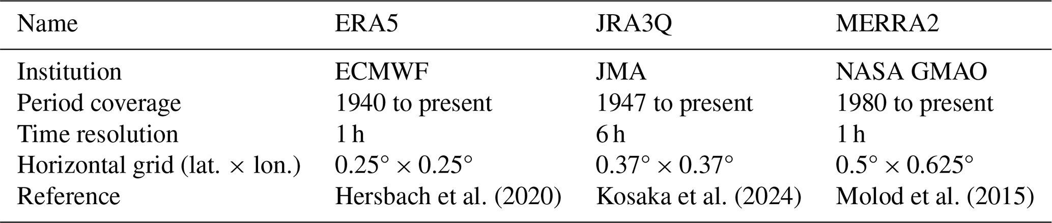
We use a subset of the latest generation of products that are commonly used in earth system research: ERA5, JRA3Q and MERRA2. The main characteristics of these reanalyses are given in Table 1. We excluded the NCEP-NCAR reanalysis as it is planned to be discontinued in 2026. We initially also included NCEP-DOE2, an update of NCEP-NCAR, but ultimately excluded it because of anomalously large wind speed biases relative to the other products. Spuriously high winds in NCEP-DOE2 have been noted previously. For example, Lucio-Eceiza et al. (2019) found that NCEP-DOE2 has worse performance than its predecessor NCEP-NCAR in estimating surface wind speeds in the North Atlantic, while Dong et al. (2020) found it had markedly worst performance in estimating Antarctic Ice Sheet winds compared to five other contemporary products.

Table 1 Basic characteristics of the reanalysis products used.

Here we briefly survey some existing assessments of our chosen reanalyses and their predecessors, focusing on the Antarctic and Southern Ocean. Though a number of past studies have evaluated reanalysis winds in the Southern Ocean, the extent of past evaluation in the near-Antarctic region remains relatively limited because of the sparsity of available in-situ measurements (Caton Harrison et al., 2022; Jones et al., 2016).

Broadly, most analysis found ERA5 performed better than, or as well as, other products when evaluated against in-situ observations. Li et al. (2013) found that ERA-Interim (a predecessor to ERA5) generally had a low bias in 10m wind speed compared to in-situ shipboard observations across the entire Southern Ocean (0.06 m s⁻¹, as compared to a high bias of 1.37 m s⁻¹ for NCEP-DOE (the predecessor to NCEP-DOE2). When Jones et al. (2016) evaluated the ERA-Interim, JRA-55 (predecessor to JRA3Q), and MERRA1 (predecessor to MERRA2) reanalyses against research vessel observations, radiosonde automatic weather station (AWS) measurements, and radiosondes in the Amundsen sea, the group found JRA-55 had the smallest wind speed biases compared to AWS and research vessel observations, while ERA-Interim showed lowest biases compared to radiosonde profiles. Overall, Jones et al. showed that all three products represented open-ocean wind speeds reasonably against observations. Caton Harrison et al. (2022) found ERA5 slightly outperformed JRA-55 and MERRA2 winds in an analysis against coastal station and Advanced Scatterometer (ASCAT) measurements, though performance was similar between reanalyses. Similarly, Dong et al. (2020) found ERA5 outperformed MERRA2, ERA-Interim, and JRA-55 against 56 meteorological stations over the Antarctic Ice Sheet. Li, Jones, and Caton Harrison all note that all reanalysis products overestimate in-situ winds at low-wind speed conditions (< ∼ 4 m s⁻¹) and underestimate them at high-wind conditions (> ∼ 25 m s⁻¹).

A global intercomparison of near-surface winds that included ERA5, MERRA2, and JRA-55 (a predecessor of JRA3Q) found ERA5 substantially outperformed the other reanalyses in reproducing in-situ observations from (land-based) tall tower platforms (Ramon et al., 2019). Based on these findings and the studies outlined above, we treat ERA5 as our benchmark reanalysis, following other Southern Ocean wind studies (e.g. Goyal et al., 2021).

2.2 Spatiotemporal standardization

We account for differing spatial and temporal resolution when comparing reanalysis products. 10 m wind speed calculated from u and v components at hourly resolution and then averaged to daily resolution is typically higher than wind speed calculated from the same u and v components that have been first averaged to daily resolution. We therefore average all u and v components to daily resolution before deriving wind speed. For similar reasons, we interpolate all three fields (u-component, v-component, and wind speed) to a standard 1° × 1° grid using the cdo package (Schulzweida, 2023). We are interested primarily in the mean state, trends, and extremes of the open-ocean circumpolar winds. As the wind jet is typically found between 48 and 54° S (Swart and Fyfe, 2012), we focus our analysis on the open water winds in the region 40 to 60° S.

Annual and seasonal means are reported by first calculating area-weighted daily mean wind speeds from the 1° × 1° gridded product for the region 40 to 60° S, then calculating the seasonal mean from these daily means. To calculate extreme high (low) wind speeds, we first calculate the daily weighted 95th (5th) percentile of winds from the 1° × 1° product over 40 to 60° S, then take the weighted average of all cells above (below) this percentile. The seasonal extreme winds are then the average of these daily extreme winds for each season in each year. We calculate linear decadal trends in mean and extreme winds from annual and seasonal values for the time periods 1980–2019 and 1980–1999, testing for significance at the 5 % level using the Wald test (Wald, 1943). We calculate the interannual variability (IAV) of each reanalysis from the annual (seasonal) means as the unbiased standard deviation of the time series, expressed as a percentage of the mean wind speed. When calculating the frequency distribution of wind speeds, we consider the full time series of area-weighted, daily mean open water wind speeds from the 1° × 1° gridded product for the region 40 to 60° S, using 100 evenly spaced bins between 0 and 20 m s⁻¹.

We use the 1° × 1° gridded products to calculate the wind jet position. At each longitude, for each day, we record the jet position as the location of the maximum of the u-component of the 10 m wind speed between 30 and 70° S, following Bracegirdle et al. (2013). We then use this daily wind jet position at each longitude to calculate the zonal average and the seasonal average. This approach introduces less variability than an alternative in which winds are first averaged seasonally before the jet is identified at each longitude and averaged zonally. A further option – taking the zonal mean of the wind speed prior to jet identification – reduces the effective resolution to 1°, limiting the ability to detect trends.

We consider a forty-year time period (1 January 1980–31 December 2019), available for all considered reanalyses; prior to 1979, satellite measurements are limited. We further separately consider the first half of the time period (1980–1999), which corresponds to the period of maximum Antarctic ozone loss (Solomon et al., 2017), and which is expected to drive wind speed increases and a poleward shift of the westerly jet.

2.3 SAM index

In each reanalysis, we calculate and then evaluate the SAM index at monthly resolution against the observational SAM index (Marshall, 2003). Following Velasquez-Jimenez and Abram (2024), the “natural”, or non-normalized, SAM index is calculated as:

$$\begin{array}{}\text{(1)}& \mathrm{SAM}=P{*}_{\mathrm{40}\mathit{°}\mathrm{S}}-P{*}_{\mathrm{65}\mathit{°}\mathrm{S},}\end{array}$$

where P*_40° S and P*_65° S are the zonal MSLP anomalies at 40 and 65° S, respectively, relative to the time period 1980–2019.

In the observational SAM index, these MSLP anomalies are calculated from the mean of six station records near each of the two latitudes for which good long-term records exist. In the reanalysis SAM index we simply use the zonal mean at both latitudes as in Gong and Wang (1999). We use the zonal mean rather than subsampling the reanalysis to the six station locations to maintain consistency with standard reanalysis-based SAM calculations (e.g. Morgenstern, 2021) and to avoid sampling biases introduced by point-location extractions from gridded fields. The zonal mean better represents the large-scale circulation patterns that define the SAM, whereas point samples can be influenced by local topographic effects and sub-grid-scale processes that are not fully resolved in reanalysis products.

Unlike the Marshall and Gong and Wang indices, the natural SAM index presented here is not normalized by dividing by the reference interval standard deviation. It is therefore not dimensionless and given in units of hPa. This approach has the advantage of making the trends and magnitude of the index less sensitive to sampling frequency.

2.4 Modelled Ozone Depletion

We perform simulations with UKESM1 to quantify the relative contribution of ozone depletion and greenhouse gas induced warming on the wind field trends. UKESM is a well-established earth system model (ESM, Sellar et al., 2020; Yool et al., 2021) based on the HadGEM3-GC3.1 coupled physical atmosphere-ocean model (Kuhlbrodt et al., 2018). We refer readers to these articles for a general evaluation of UKESM1, and only highlight here components of the model that are central to our work. The atmospheric component of UKESM1 is the Global Atmosphere 7.1 (GA7.1) science configuration of the Unified Model (Walters et al., 2019), with horizontal resolution of approximately 135 km (1.25° × 1.875°), 85 vertical levels and a model top located at 85 km altitude. Unusually for a CMIP6 model (Coupled Model Intercomparison Project Phase 6; Eyring et al., 2016), UKESM1 simulates full atmosphere ozone chemistry through the UK Chemistry and Aerosols (UKCA) model (Archibald et al., 2020; Mulcahy et al., 2018), interactively coupled to the model's physics and dynamics. Ozone is therefore prognostic, with its evolution dependent on, and influencing, the simulated atmospheric thermal, dynamical and chemical states (Keeble et al., 2021).

The ability of UKESM1 to simulate the historical and future evolution of ozone has been discussed in Keeble et al. (2021), Morgenstern et al. (2022) and Zeng et al., (2022), while representation of the SAM in CMIP6 models (including UKESM1) has been analysed by Morgenstern (2021). UKESM1 overestimates the observed global mean total column ozone (TCO) over the period 1980 to 2015, with this overestimation reduced over the Antarctic region (60 to 90° S). In addition, UKESM1 has a stronger negative TCO trend globally than observed, with this overestimate also reduced for the 60 to 90° S region. The bias in UKESM1 trends in TCO (discussed further in Sect. 3.3) should be kept in mind when the impact of ozone depletion and recovery on surface winds is discussed.

2.5 CMIP6 model intercomparison

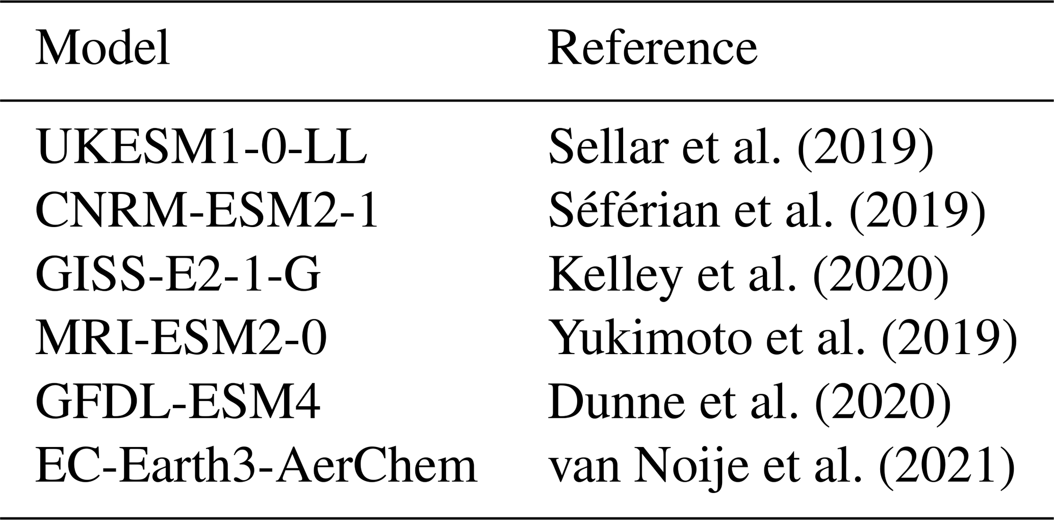
To contextualize UKESM1 results, we report trends in the winds and the SAM index, as well as in total column ozone (TCO), for other CMIP6 models with interactive chemistry for which SAM, TCO, and (at least) daily-resolution wind fields are available (Table 2). Spatiotemporal standardization and SAM index calculation is performed as described in Sect. 2.2 and 2.3. For the intercomparison of the subset of CMIP6 models, we use the historical run for the period 1980–2014 and the SSP 3-7.0 run for the period 2015–2019. We calculate trends in SAM, 10 m wind speed, and total column ozone (TCO) for the band 70–90° S, for 1980–1999 and 1980–2019.We compare CMIP6 TCO trends to an observational dataset (Bodeker et al., 2021). For this intercomparison, to maintain consistency in method, only one ensemble member of each model, including UKESM1, is used.

Table 2 CMIP6 models with interactive chemistry used in the intercomparison. Only models with both interactive chemistry and 10 m wind fields available at (at least) daily resolution are used. One ensemble member is used per model.

2.6 Experimental Design

Morgenstern (2021), Revell et al. (2022) and Zeng et al. (2022) emphasize that to simulate forced trends in Southern Ocean winds models need to interactively simulate ozone chemistry, GHGs and ODS. This is to capture multiple interactions between GHGs (e.g. CO₂, CH₄, N₂O), ozone, and their combined impact on model dynamics. Prescribing an externally generated ozone field risks it being chemically inconsistent with other time-evolving GHGs (Zeng et al., 2022), and potentially be offset with respect to the model thermodynamical fields (Morgenstern, 2021). Morgenstern (2021) shows that the CMIP6 DAMIP (Detection and Attribution Model Intercomparison Project) experiments (Gillett et al., 2016); hist-GHG (historical GHG forcings with all other forcings pre-industrial) and hist-stratO3 (prescribed historical ozone and all other forcings pre-industrial) do not combine to give the (forced) time evolution of the SAM index seen in full historical simulations. This is due to feedbacks between the time-varying GHGs and ozone leading to a different impact on model dynamics compared to the combination of the two individual drivers. This feedback is captured in models that run with interactive chemistry.

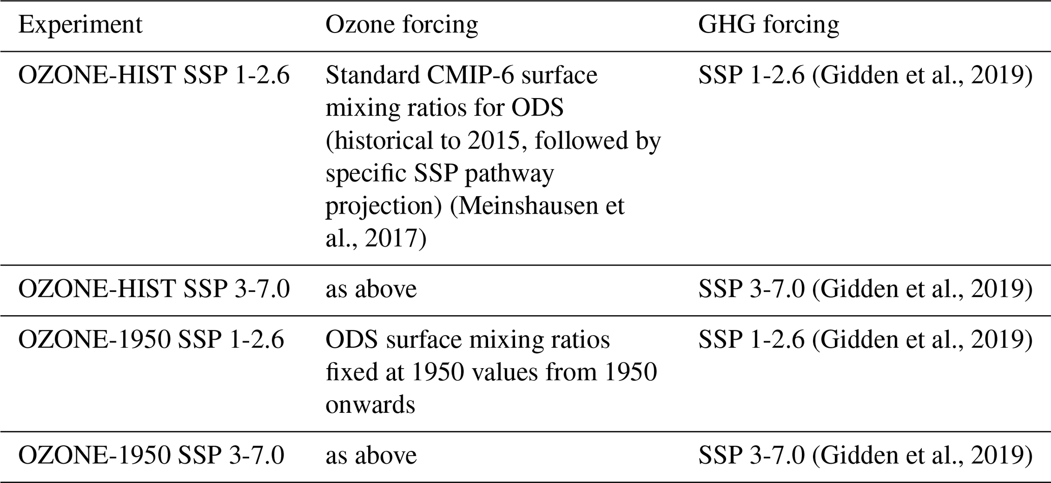
Motivated by these studies, we use UKESM1 with interactive chemistry to study the role of stratospheric ozone loss and recovery on Southern Ocean winds. We control the evolution of stratospheric ozone in UKESM1 by modifying surface mixing ratios of ozone depleting substances (ODS, e.g. chlorofluorocarbons and hydrochlorofluorocarbons), which play a central role in driving stratospheric ozone loss (Farman et al., 1985; Solomon et al., 1986). We perform simulations for 1950 to 2100 using two ODS surface mixing ratio scenarios: (i) ODS use the standard CMIP6 surface mixing ratios (historical followed by a projection), and (ii) ODS are fixed at 1950 values. We refer to these two experiments as OZONE-HIST and OZONE-1950. OZONE-HIST results in ozone loss from approximately 1970 to 2000, followed by a slow recovery through to 2100 (Keeble et al. 2021, Fig. 7). OZONE-1950 minimizes stratospheric ozone loss throughout the simulation as only trace amounts of ODS, emitted or produced in the atmosphere before 1950, are available for ozone destruction in the stratosphere.The two ODS scenarios are combined with two CMIP6 SSP scenarios (SSP 3-7.0 and SSP 1-2.6; Gidden et al., 2019) that represent a high and low GHG emission scenario.

This configuration results in four experiments that allow us to isolate the effects of simulated stratospheric ozone and GHG on wind trends; see Table 3 for a summary. Following McLandress et al. (2011), we assume that ozone-driven trends (resulting from the different ODS surface mixing ratios) and GHG-driven trends are additive; that is, the OZONE-HIST run demonstrates a linear addition of ODS-driven trends and GHG-driven trends, so [OZONE-HIST – OZONE-1950] will isolate the ODS-driven trend, while any trends in the OZONE-1950 runs are due to GHG emissions alone. We acknowledge the potential for some non-linear interactions that may weaken this assumption but suggest to first order it is a reasonable approximation for attributing the primary differences identified either to ODS or GHG differences in the respective experiments.

Table 3 Summary of experiments with description of ozone and GHG forcing.

For each UKESM1 experiment, we run three ensemble members, each branched in 1850 from the CMIP6 UKESM1 piControl following the procedure for generating initial conditions outlined in section 4 of Sellar et al., (2020). With respect to means and trends, we report the ensemble mean value, calculated at daily 1° × 1° resolution. When reporting extreme values, interannual variability, jet position, and standard deviation in the jet position, we calculate them for each ensemble member separately and give the mean of these calculations.

3 Results

3.1 Reanalysis Intercomparison

3.1.1 Wind climatology and distribution evaluation

We intercompare the reanalyses both to identify their utility for applications such as forcing ocean-only models, and to provide a baseline against which to evaluate the UKESM1 historical simulation. All the reanalysis products feature a prominent band of high winds between 40 and 60° S, with intensification over the Indian Sector (Fig. 1). MERRA2 agrees with ERA5 at high latitudes, but is evenly low compared to ERA5 over the open ocean. JRA3Q is generally higher than ERA5 (Fig. 1).

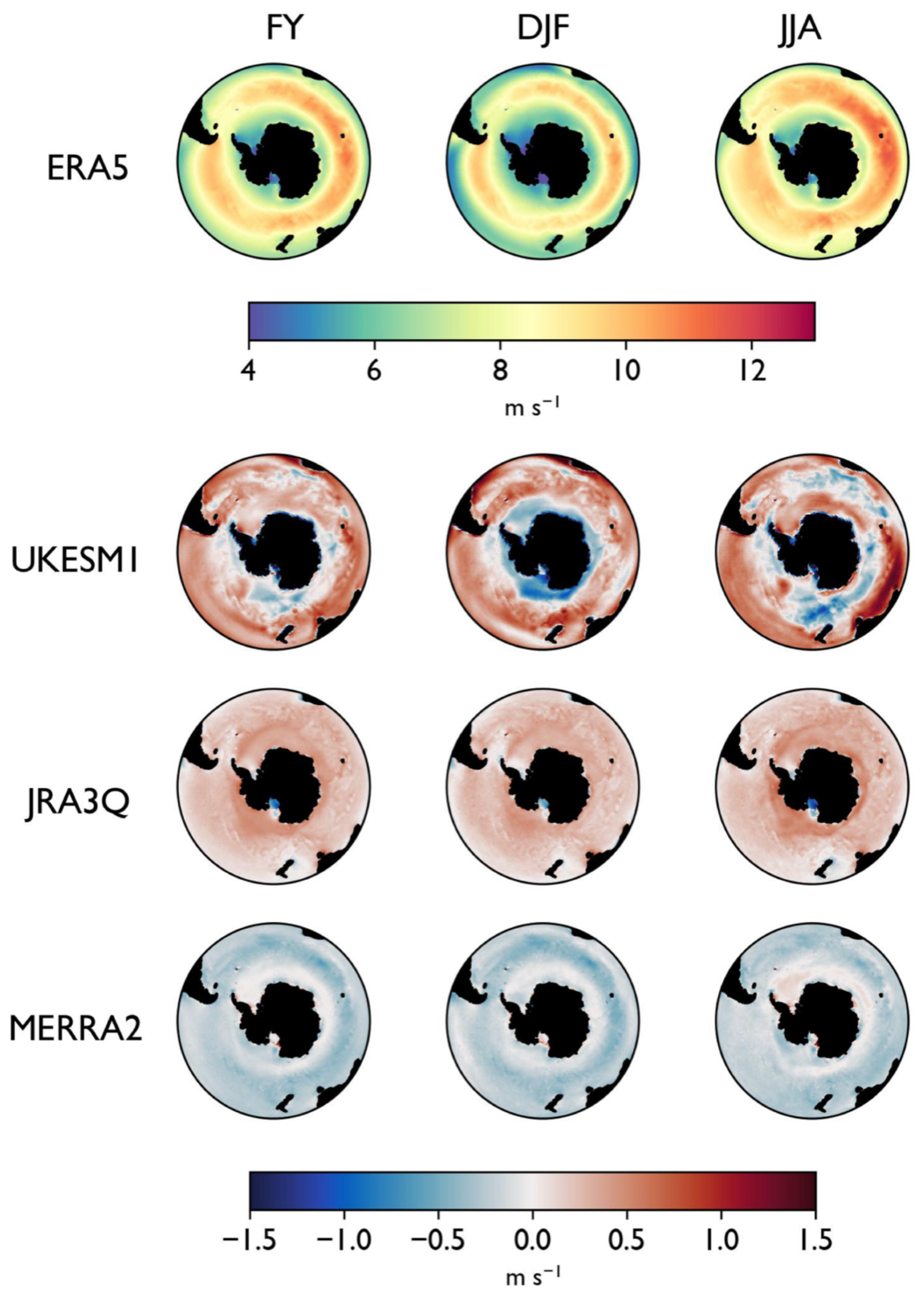
Figure 1 Climatological wind speed for 1980–2019. For ERA5, the climatological wind speed for the full year and austral summer (DJF) and winter (JJA) is shown. For the other two reanalyses and UKESM1, differences from ERA5 are shown as [product x – ERA5]; i.e. positive (red) values indicate higher winds than ERA5. See also Table 4.

The reanalysis products generally agree when considering only open-ocean winds between 40 and 60° S. Most reanalyses are relatively similar to ERA5, ranging from a difference of −0.20 m s⁻¹ (MERRA2) to +0.28 m s⁻¹ (JRA3Q) for annual-average winds. In comparison, NCEP-DOE2, excluded from this analysis for high bias, has a bias of +1.31 m s⁻¹ for yearly-averaged winds in the same region. Interannual variability (IAV) is relatively consistent but varies somewhat between reanalyses, ranging from 1.2 % in ERA5 to 1.80 % in MERRA2 (Supplement Table S1). No strong seasonal differences in interannual variability are seen in any reanalysis.

The frequency distribution of the daily winds is remarkably similar between the reanalyses (Fig. 2, Table S2), with differences mostly visible at the tails of the distribution. ERA5 has the lowest “low” (5th percentile) winds, but the other reanalyses have “low” winds only slightly (∼ 0.1 m s⁻¹) higher than ERA5. There is more spread at the high end of the distribution, where ERA5 sits in the middle of the reanalysis set and year-round differences from ERA5 range from −0.35 m s⁻¹ (MERRA2) to 0.59 m s⁻¹ (JRA3Q).

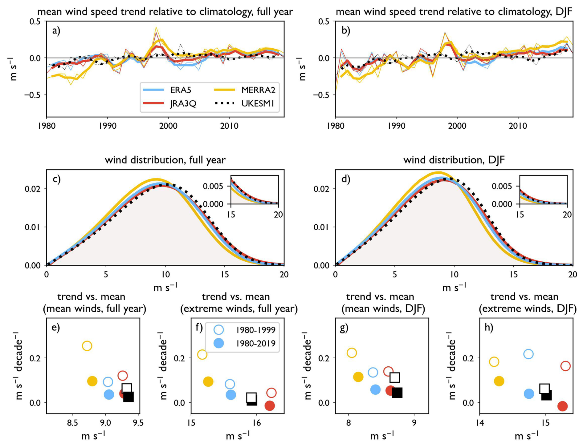
Figure 2 Summary statistics for wind distributions in four reanalysis products and UKESM1. (a–b) mean 10 m wind speed trends relative to climatology for (a) full year and b) DJF only. Thick lines have been smoothed by a three-point running filter. (c–d) windspeed frequency distribution (100 bins, 0–20 m s ⁻¹) for (c) full year and (d) DJF, with high tails shown in inset. (e–h) Trends in mean and extreme winds for full year and DJF vs. climatological means, with colours the same as in panel a). Filled symbols represent 1980–2019, while open symbols represent 1980–1999; circles represent reanalyses while squares represent UKESM1. Colours from panel (a) are repeated throughout the figure. Summary statistics shown in panels (e)–(h) are also given in Tables 4 and 5. All figure statistics are calculated for daily winds at 1° × 1° resolution, 40–60° S.

3.1.2 Wind speed trends

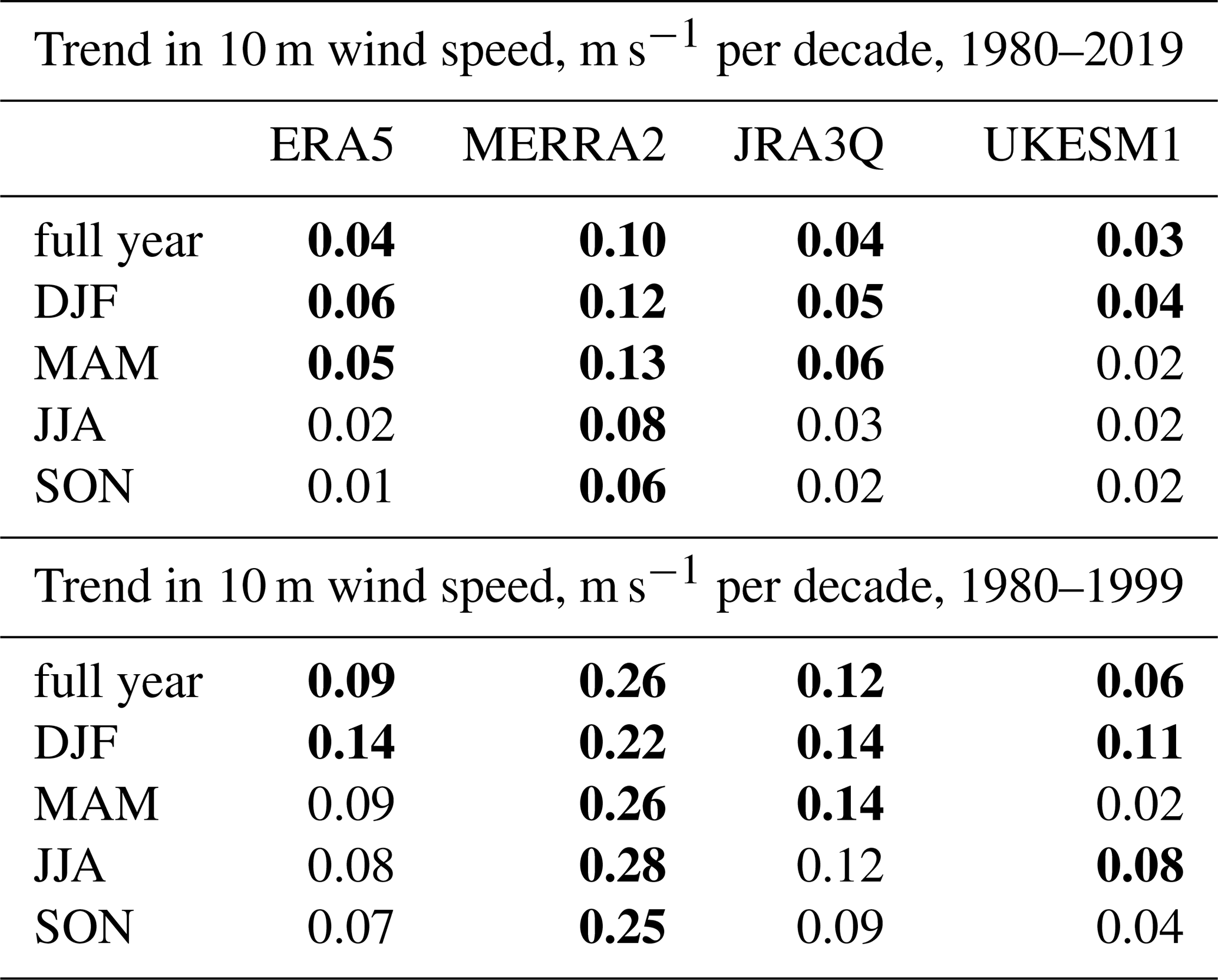
Trends in open-ocean wind speed differ between the reanalyses much more than the climatological mean fields (Figs. 2a–b, 3, Table 5). JRA3Q and ERA5 behave similarly over the whole time period (1980–2019), having a statistically significant year-round mean trend of ∼ 0.04 m s⁻¹ per decade that is slightly stronger in austral summer and autumn and not statistically significant in winter (JJA) and spring (SON). In contrast, MERRA2 has much stronger trends – ∼ 2.5× the magnitude of the ERA5 annual mean tren. The seasonality in this reanalysis is also very different from ERA5, with relatively strong, statistically significant trends persisting year round. Trends in MERRA2 are also statistically significant over a much larger area of the Southern Ocean, as well as in the JJA season (Fig. 3).

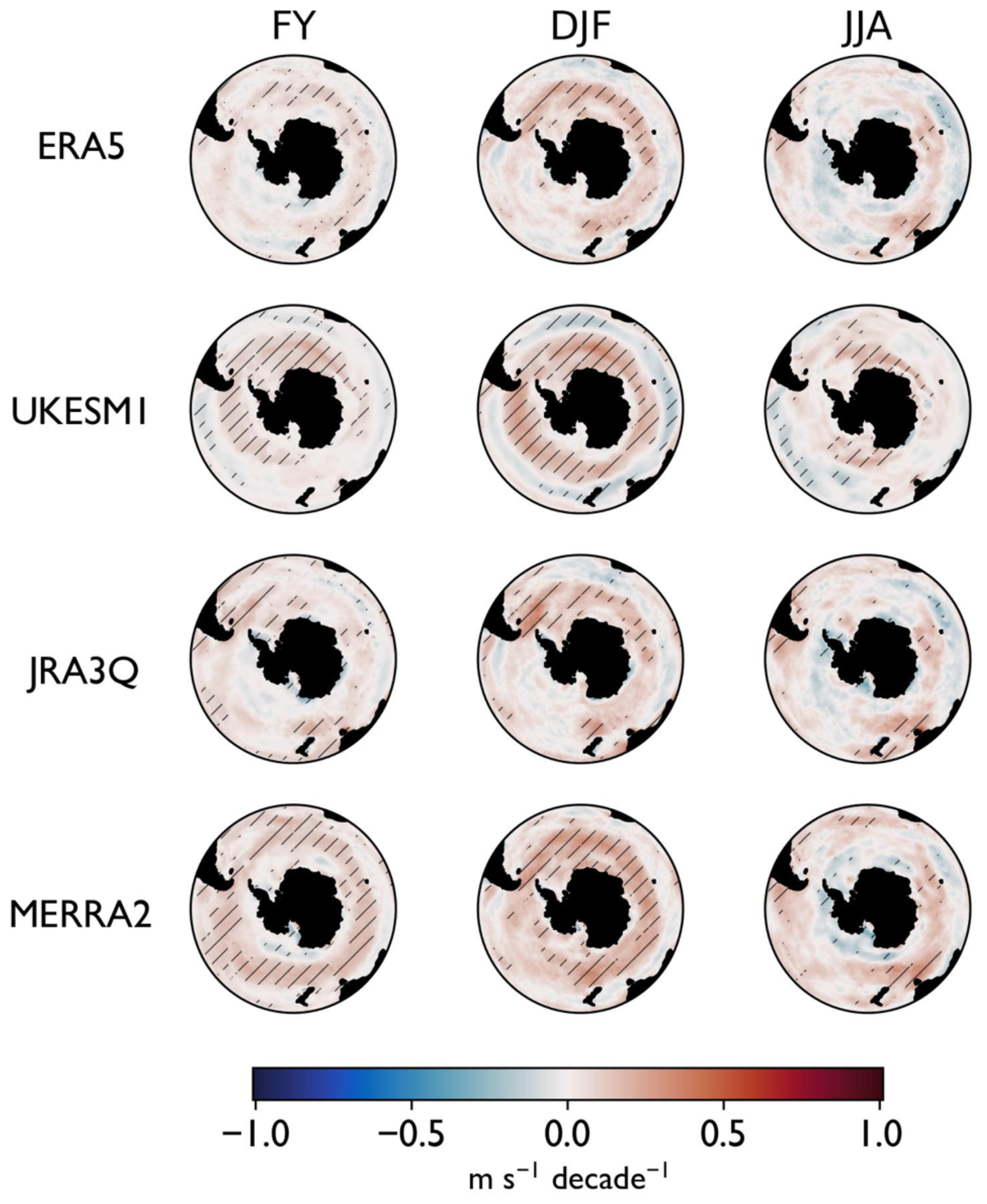
Figure 3 Decadal trends in 10 m wind speed (1980–2019). Hatching shows trends significant at the 95 % confidence level. See also Table 5.

Summer (DJF) mean wind speed trends in the period of maximum ozone depletion (1980–1999) are approximately double those for the full time period in all reanalyses (Fig. 2, Table 5). Trends in the extreme winds follow a similar pattern to the mean winds, with MERRA2 trends much stronger than those of JRA3Q and ERA5 (Fig. 2e–h). Trends in extreme winds are not systematically stronger than trends in mean winds and are less likely to be statistically significant.

3.1.3 Jet position and poleward trend

The annual average zonal mean wind jet sits at 52.1° S in ERA5 and is similar between products (Fig. 4, Table S3). The jet position exhibits a substantial seasonal cycle, being at its most southerly location in austral autumn and most northerly location in austral spring. All reanalyses represent this seasonal cycle in the jet position, with an approximate amplitude (of the seasonal averages) of ∼ 1.6°. Interannual variability of the mean jet position over the time period 1980–2019 is comparable between reanalyses – with a standard deviation of the zonal mean of approximately 0.8° (MERRA2). The zonally-varying standard deviation of the jet position (shown in Fig. 4 only for ERA5, for clarity) is also comparable. The strongest poleward trend in the wind jet occurs in austral summer and autumn, and is much stronger (1.8$\times -\mathrm{3.8}\times$) during the period of maximum ozone depletion (1980–1999) than over the whole time period (Table S4). Trends in the position of the jet are not always statistically significant in the reanalyses because of the large interannual variability.

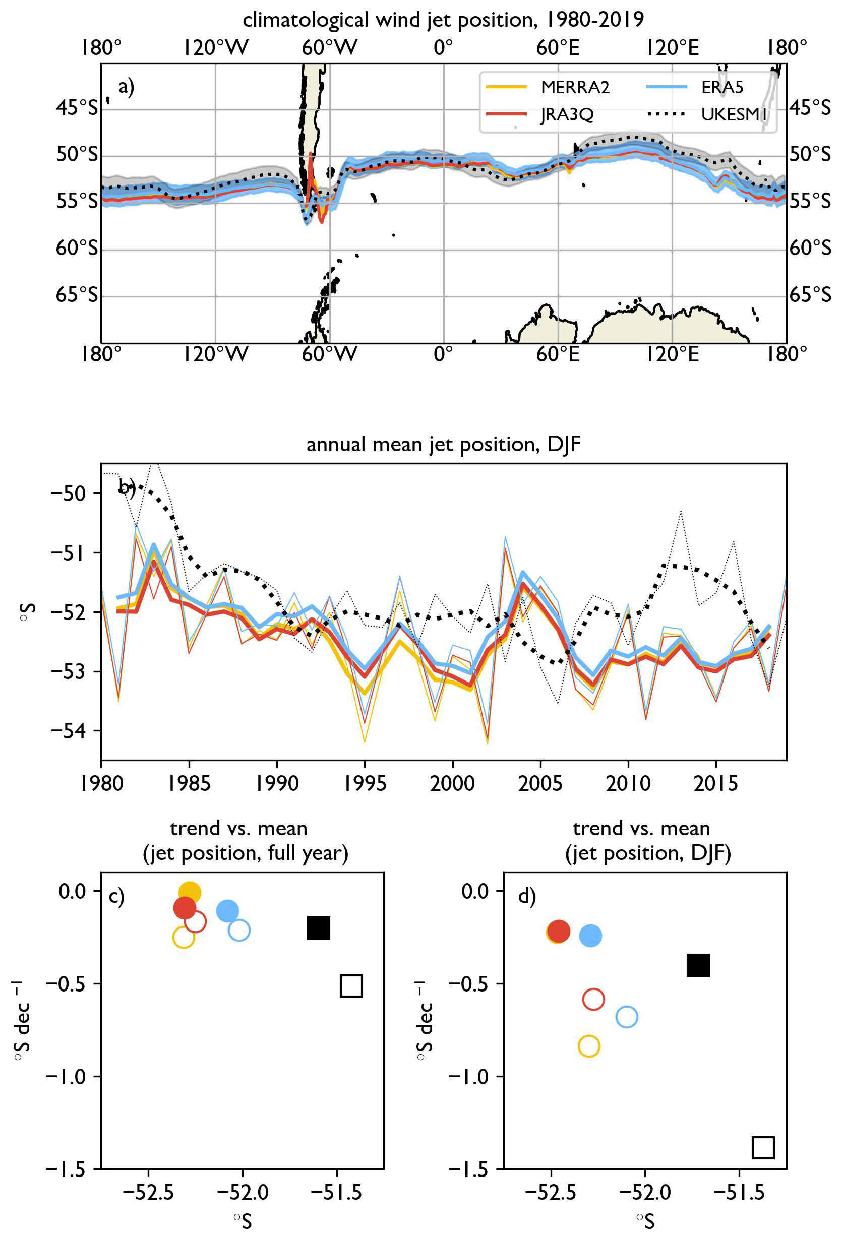
Figure 4 Summary statistics for the wind jet. The wind jet is calculated as the location of the maximum of the u-component of the 10 m wind speed between 30 and 70° S (see Methods). (a) the climatological mean annual jet position, with one standard deviation of the annual mean shown for ERA5 and UKESM1. (b) The zonal mean of the austral summer jet position. Thick lines indicate smoothing by a 3-point running mean filter. (c–d) Trends in the annual (c) and summer (d) jet position mean vs. climatological means. Colours from panel (a) are repeated throughout the figure. See also Tables S3 and S4.

3.1.4 SAM index

The timeseries of the station-based SAM index (see Methods) provides a possible observational constraint on the accuracy of the reanalysis products. The SAM indices derived from reanalyses exhibit a high temporal coherence with the observational SAM index, with some deviations – for example in JRA3Q during 2005–2010 (Fig. 5). The trend in the SAM index has a seasonal character both in the observations and in the reanalyses. It is strongest in austral summer (DJF) and autumn (MAM), and typically much weaker and not statistically significant in the other seasons (Fig. 5, Table S5). The observational trend is much stronger in the period of maximum ozone loss than in the whole time period (factor of ∼ 3×), which is reflected in the reanalyses (factor of ∼ 2.3–3.6×).

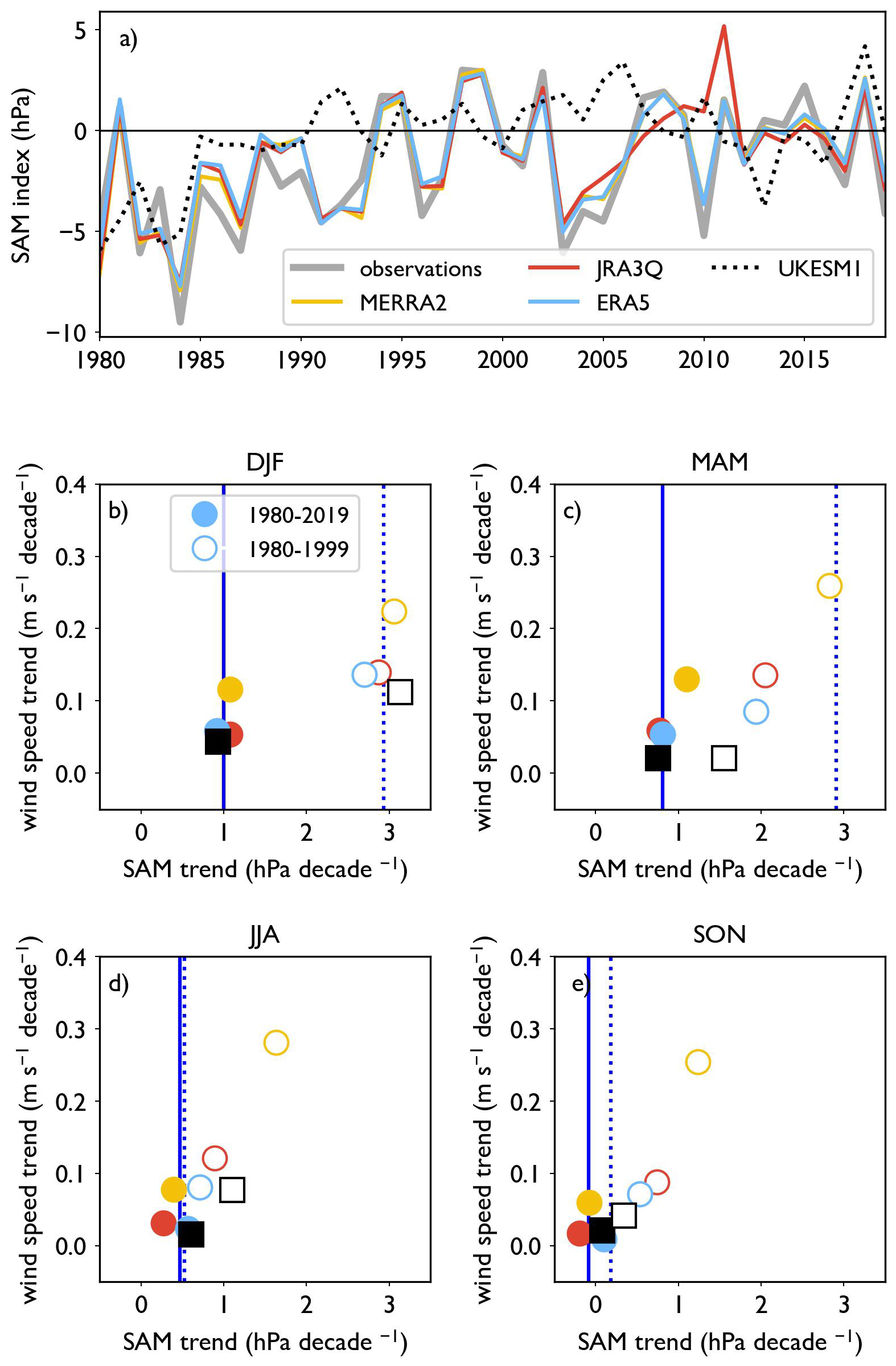
Figure 5 Summary statistics for the SAM index. (a) Timeseries of the austral summer (DJF) SAM index. To highlight coherence of interannual variability, no running-mean filter has been applied. (b–e) Trends in the wind speed vs. trends in the SAM index, subdivided by season. Filled symbols represent 1980–2019, while open symbols represent 1980–1999. Vertical lines show the observational SAM index (full line represents 1980–2019, dotted line represents 1980–1999). Colours from panel a) are repeated throughout the figure. See also Table S5.

In all seasons, the trend in the SAM index in the reanalyses correlates tightly with the trend in the estimated wind speed (r= 0.72–0.93, p<0.05). Because the wind acceleration is mechanistically linked to the trend in the SAM, evaluating the accuracy of the reanalysis-derived SAM indices against the observational index may provide a constraint on the accuracy of reanalyzed wind speed trends; i.e. a trend in the SAM should result in a trend in the wind speed. Notably, this observational SAM constraint suggests that the strong trends in the MERRA2 reanalysis in austral winter and spring over the period of maximum ozone depletion may be spurious, as they are accompanied by strong SAM index trends that are not present in the observations (Fig. 5, panels d and e). Additionally, in autumn, the ERA5 and JRA3Q time series appear to underestimate the SAM trend during 1980–1999, while MERRA2 overestimates it over the course of the whole time series, suggesting possible corresponding overestimations/underestimations of the respective wind trends. In summer, the observational constraint appears to have less power, as the reanalyses show a variety of wind speed trends while all representing the SAM relatively accurately (Fig. 5b).

3.1.5 Reanalysis intercomparison summary

All four reanalyses show relative coherence in mean wind speed climatology, distribution, jet position and jet seasonal cycle. Moderate differences in extreme winds, interannual variability and jet latitudinal trend are observed. Reanalyses tend to exhibit systematic biases in capturing the tails of the observational wind distribution (i.e., they overestimate extremely low winds and overestimate extremely high winds relative to observations; see summary of previous in-situ evaluation in Methods). Thus, it is plausible that ERA5, which has the lowest extreme low winds, is the best representation of the low tail of the distribution, while JRA3Q may be the best at representing high winds.

The most important differences between the reanalysis products are in the representation of the wind speed trends over the time period 1980–2019. MERRA2 has considerably stronger trends than ERA5 and JRA3Q, and moreover these trends persist year round. To evaluate which trends seem more plausible, we consider an observational constraint in the form of the observational SAM index. MERRA2 appears to overestimate SAM index trends, especially in austral winter and spring, suggesting that their strong wind trends in these time periods may be spurious. This provides additional rationale for using ERA5 as the baseline reanalysis against which to evaluate the UKESM1 model at southern high latitudes.

3.2 UKESM1 evaluation against reanalyses

We next evaluate the main Southern Ocean wind features in UKESM1 against our default reanalysis, ERA5, to assess the model's suitability for answering scientific questions related to changing wind patterns in this region. The UKESM1 model has an overall year-average positive bias of ∼ 0.3 m s⁻¹ relative to the ERA5 climatology in the band between 40 and 60° S (Fig. 1), which does not vary substantially by season (Table 4). UKESM1 underestimates winds at high latitudes compared to ERA5 while showing the strongest positive bias over the mid-latitude open ocean. However, on average, the UKESM1 distribution is similar to that of ERA5, though slightly shifted towards higher winds than the reanalyses in the middle of the distribution (Fig. 2). Extreme low (5th percentile) winds are nearly identical to ERA5 values, while the highest winds are somewhat higher (∼ 0.3 m s⁻¹, S2).

Table 4 Climatological 10 m wind speed (1980–2019). Seasonally subdivided open-ocean wind speed between 40 and 60° S for ERA5, and differences from ERA5 for the other reanalyses and UKESM1.

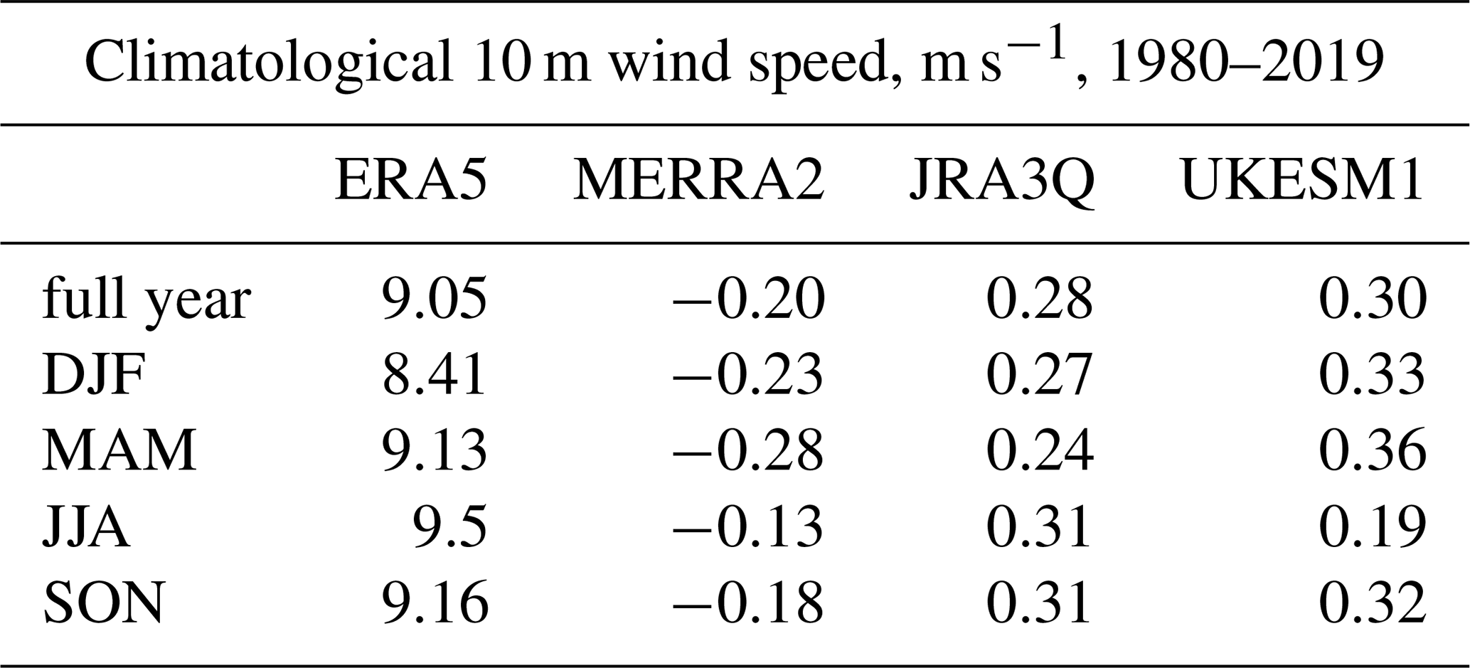
Table 5 Decadal trends in 10 m wind speed. Seasonally subdivided trends in open-ocean wind speed between 40 and 60° S are shown for 1980–2019 and 1980–1999. Trends significant at the 5 % level are given in bold.

Interannual variability in UKESM1 is comparable to that of ERA5, with an average ratio of 0.8 (IAV_UKESM1 $/$ IAV_ERA5) for annual values (S1).

UKESM1 has similar decadal trends in wind speed to ERA5, with strongest acceleration in austral summer (0.04 and 0.06 s⁻¹ per decade for for UKESM1 and ERA5, respectively, over 1980–2019, as compared to 0.11 and 0.14 s⁻¹ per decade over 1980–1999; Table 5). The general pattern of significant wind trend strength peaking in austral summer is consistent between the model and ERA5. Spatial patterns (significant acceleration occurring mostly in the 40–60° S band, and more visible in austral summer, Fig. 3), are also reproduced by the model.

The UKESM1 jet position is similar to that of ERA5 (Fig. 4, Table S3) and accurately captures the observed seasonal cycle in position (most southerly in MAM, most northerly in SON). The majority of the temporal variability in jet location is a result of natural variability (as opposed to from a forced signal, such as ozone depletion). We would therefore not expect a free running model like UKESM1 to capture the temporal evolution of this variability. (We would, however, expect the model to capture any externally forced, longer-term trends.) The magnitude of variability in the jet location is comparable between UKESM1 and ERA5, as seen in the zonally-varying standard deviation for 1980–2019 (Fig. 4). The UKESM1 trends in the poleward position of the jet are much stronger than in the reanalyses over the whole time period (∼ 1.8× ERA5 in the annual mean, ∼ 1.7× ERA5 in the DJF mean, Table S4), a feature that is amplified in the period of maximum ozone loss (1980–1999, Table S4). This feature is likely due to Antarctic ozone loss being higher in UKESM1 than observed (Keeble et al., 2021, and Sect. 3.3 of this paper).

The variability and trend in the SAM index is comparable to that of ERA5 and observations (Fig. 5, Table S5). As in the case with the jet position, UKESM1 does not reproduce the time variation in the SAM index seen in the reanalyses because of the significant role played by natural variability. Trends in the SAM index during 1980–1999 are much (up to ∼ 3×) stronger than those during 1980–2019, both in the ERA5 reanalysis and in UKESM1. Similar to ERA5 and JRA3Q, in both time periods, UKESM1 has strongest, most significant SAM trends during DJF and MAM, accompanied by stronger wind acceleration in those seasons (Fig. 5). In particular, UKESM1 accurately captures the SAM trend in DJF, including the differential trends between the full period and the shorter 1980–1999 period. This differential response is less accurately captured in MAM, although the SAM trend for the full period is well simulated.

Overall, the UKESM1 Southern Ocean wind climatology and distribution, including extremes, as well as decadal trends wind speeds and the SAM index, are remarkably consistent with that of ERA5; however, mean wind speeds are somewhat higher in the model. The mean jet position is also reproduced, though UKESM1 demonstrates stronger poleward movement than all reanalyses.

3.3 UKESM1 in the context of CMIP6 models with interactive chemistry

The CMIP6 models with interactive ozone show substantial spread (∼ 1 m s⁻¹) in their representation of the mean wind speed over the Southern Ocean (Fig. 6a–c). All models, except GISS-E2-I-G and EC-Earth3-AerChem, overestimate the climatological mean wind speed with respect to ERA5, with UKESM1 within the spread of other models. Agreement across the models in wind speed trends is also generally weak. Most models (except MRI-ESM2-0) show larger DJF trends for 1980–1999 than 1980–2019, with GFDL_ESM4 and UKESM1 being notably accurate for both time periods. Furthermore, all models except UKESM1 underestimate the JJA wind speed trend during 1980–1999, though trends in this season are not expected to be strongly forced by ozone trends. UKESM1 performs well in capturing wind trends compared to other CMIP6 models, reproducing relatively well the wind speed trends seen in ERA5, for DJF and JJA, for both time periods considered, including differences between the two periods.

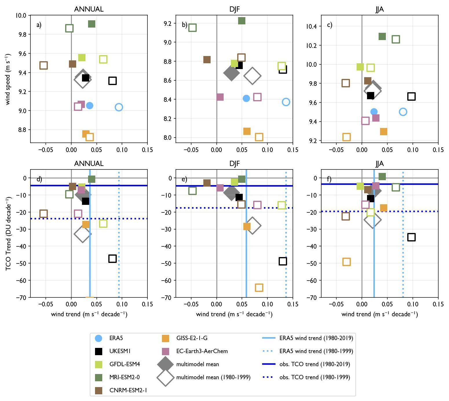
Figure 6 10 m wind speed, decadal wind speed trend, and decadal TCO trend (70–90° S) for CMIP models with interactive chemistry. For each model, one ensemble member is used (see Table 2). Wind speeds and trends are calculated from daily winds at 1° × 1° resolution, 40–60° S. Note the caveats regarding TCO trends in GISS-E2-I-G discussed in Sect. 3.4.

On average, the models overestimate TCO depletion (for the area 70–90° S), though with considerable inter-model variation: MRI-ESM2-0 underestimates depletion, GFDL-ESM4, EC-Earth3-AerChem, and CNRM-ESM2-1 are quite accurate, while UKESM1 and GISS-E2-1-G substantially overestimate ozone loss across all seasons and time periods (Fig. 6 lower panels, Fig. S1 in the Supplement). Though stronger ozone depletion is expected to correlate with larger wind speed trends, this relationship holds only partially in austral summer. GISS-E2-1-G substantially overestimates ozone depletion in 1980–1999, but fails to produce a correspondingly strong wind speed trend, even in summer. Note that GISS-E2-1-G is known to have biases in simulating the recovery of volcanic eruptions, which amplifies the influence of ODS on TCO, so while we include it in the comparison of models, we keep this bias in mind when interpreting results. Similarly, CNRM-ESM2-1 reasonably captures the observed ozone loss but underestimates wind speed trends. GFDL-ESM4 best matches both metrics in austral summer but not winter. While the strongest ozone loss typically occurs in austral spring (SON), inter-model TCO trends and their relationship with wind speed trends are consistent whether wind speed trends in DJF are plotted relative to TCO trends in SON or DJF (Fig. S2). To maintain consistency with the rest of this study, we therefore present only DJF results in Fig. 6.

UKESM1 overestimates ozone depletion, primarily in the 1980–1999 period, but accurately reproduces the ERA5 wind speed trends for both periods, suggesting the dynamical link between Antarctic ozone loss and near-surface westerlies is weaker in UKESM1 than in reality. The weak TCO–wind relationship across models in austral winter (JJA) for 1980–1999 indicates observed wind increases during this period are likely not ozone-driven. As in the reanalyses (Fig. 5), SAM trends correlate strongly with wind speed trends across CMIP6 models (Fig. S3), due to the mechanistic link between these metrics. While acknowledging recent trends in Antarctic TCO are larger than observed in UKESM1, our analysis of wind speed and SAM trends, and the implied response to ozone forcing, suggests UKESM1 is suitable for studying (and attributing) past and future changes in Southern Ocean winds, and by extension the drivers of changes in Southern ocean carbon uptake, as carried out in our earlier study (Jarníková et al., 2025).

3.4 Attribution of wind speed trends to GHG and ozone forcing with UKESM1

Finally, we use UKESM1 to attribute past, and potential future, changes in the Southern Ocean wind regimes to either stratospheric ozone changes or greenhouse gas forcing. We do this by combining two ODS scenarios (ODS-HIST and ODS-1950) with two CMIP6 emission scenarios: SSP 1-2.6 and SSP 3-7.0 for the period 1950 to 2100 (see Methods). For each experiment, we show all three model ensemble members, as well as the ensemble mean.

Over the full time period, winds increase in all seasons and scenarios (Fig. 7). The most prominent feature in the time series is a sharp increase in wind speeds in the scenario with historical ozone depletion (OZONE-HIST), approximately during 1980–2000, occurring predominantly in austral summer (DJF) and to a lesser extent in austral spring (SON; Fig. 7). During the same time period, we observe no wind increase in the scenario without ozone depletion – in fact, a minor decrease is seen (Fig. 7, Table S6). We first partition the attribution of the observed historical wind changes to greenhouse gas emissions and ozone forcing, comparing them with those seen in ERA5, and then consider potential changes over the 21st century, again attributing changes to ozone forcing and/or greenhouse gas emissions.

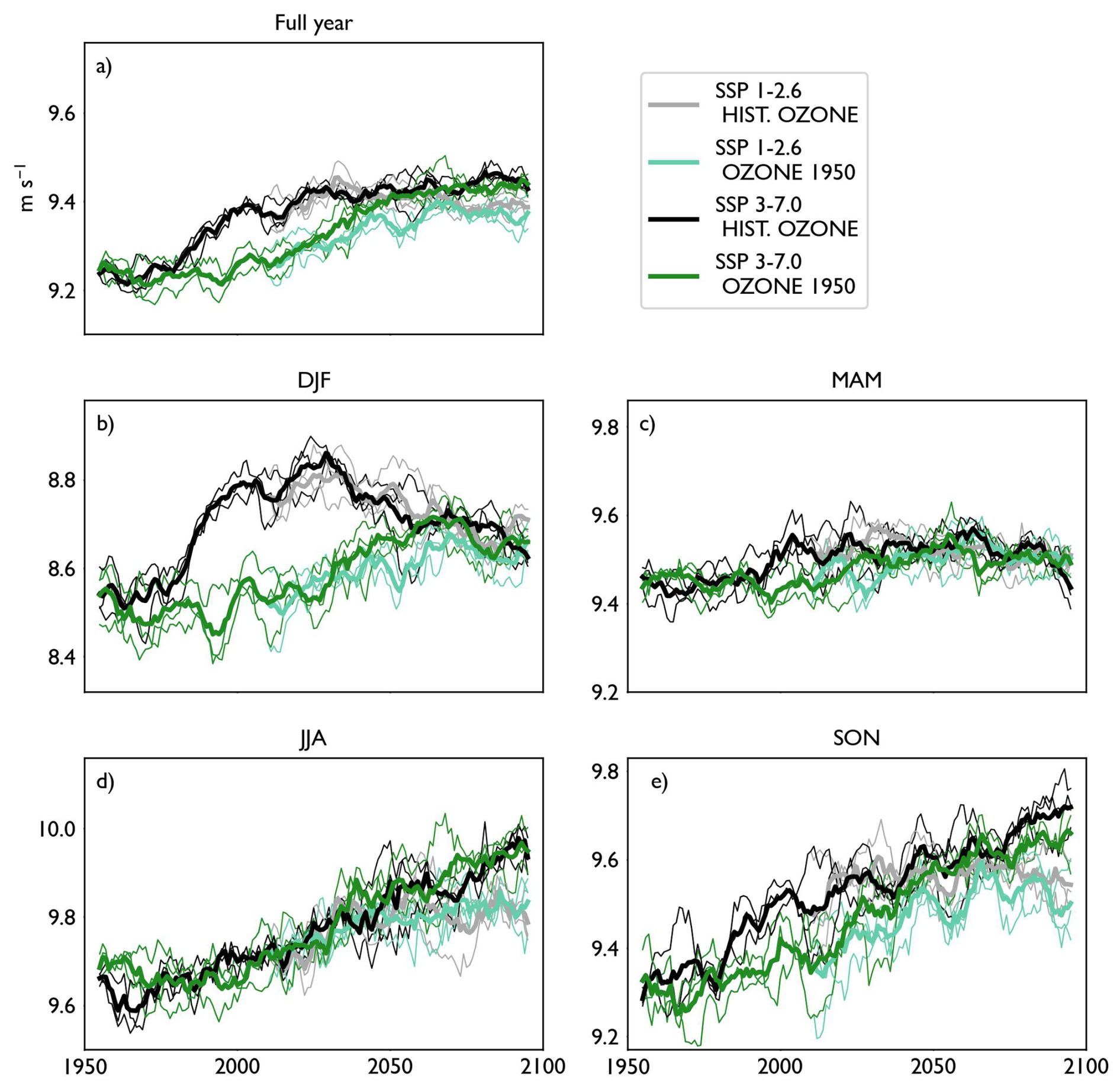
Figure 7 10 m wind speed evolution from 1950 to 2100 in the OZONE-1950 and OZONE-HIST experiments. (a) Full year, (b–e) seasonally subdivided means. All means are calculated for daily winds at 1° × 1° resolution, 40–60° S. For each experiment, three ensemble members are shown, with the ensemble mean shown in bold. All lines are smoothed with a 10-year running filter. See also Table 6.

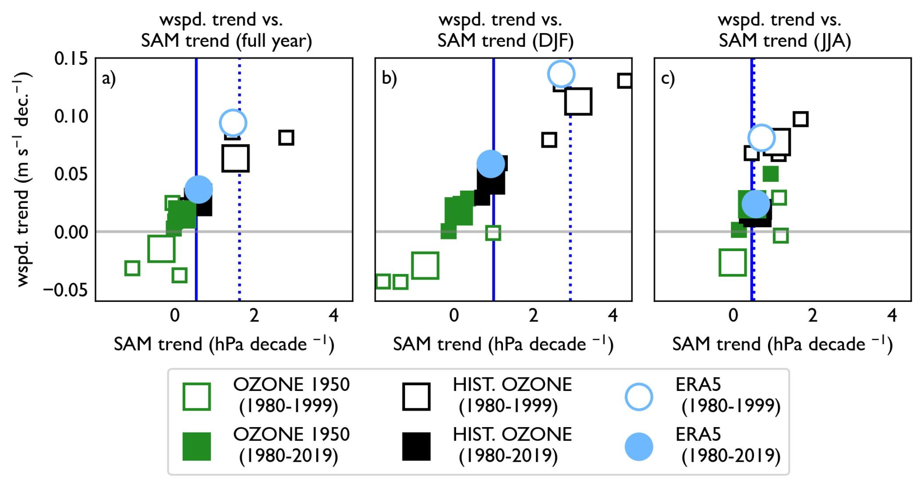
Figure 8 Trends in mean wind speed vs. trends in the SAM index for the OZONE-1950 and OZONE-HIST experiments. ERA5 is shown for comparison (blue circles), and the observational SAM index is shown as vertical lines (full for 1980–2019, dotted for 1980–1999). For the OZONE-1950 and OZONE-HIST experiments, individual ensemble members are shown as smaller squares, while the ensemble mean is shown as a larger square. As in Figs. 2, 4, and 5, filled symbols represent 1980–2019, while open symbols represent 1980–1999.

UKESM1 exhibits the same positive relationship between the trend in the SAM index and wind speed that was seen in the reanalyses. Wind acceleration (deceleration) corresponds to a positive (negative trend) in the SAM index in all ensemble members of the two experiments over the historical period (Fig. 8). Though absolute wind speeds are higher in UKESM1 than in ERA5, the magnitude of the trends in the SAM index and wind speeds, for both periods, are very similar in both datasets for all seasons (Fig. 8, Table 5), suggesting the forced signal of ozone depletion in UKESM1 captures real-world dynamics.

The key role of ozone in driving the historical SAM and wind speed changes becomes further apparent when comparing the OZONE-HIST and OZONE-1950 runs: all three ensemble members of the OZONE-1950 experiment show a much weaker wind speed trend over the whole time period (Fig. 8, filled green squares) and a negative trend over the period of maximum ozone depletion (empty green squares). Meanwhile, the OZONE-HIST runs (black squares) agree with both ERA5 and the observational SAM index over both the whole time period (filled black squares) and the period of maximum ozone depletion (empty black squares), with the differential response in DJF between these two periods, in both the SAM index and wind speeds, particularly well captured.

The general congruence of the historical UKESM1 runs with ERA5 suggests that UKESM1 captures both the sensitivity of the wind and SAM response to the time-varying trend in the ozone forcing, as well as the seasonality of this response. Both wind and SAM trends are stronger over the period of maximum ozone depletion than over the full time period, and changes in the austral summer mean are larger than in the annual mean, with minimal changes in austral winter.

We next attribute the wind changes throughout the whole simulation period 1950–2100 to either ozone or GHG forcing, subdividing the time series into three 50-year periods. In the latter half of the 20th century (1950–1999; Table 6), winds accelerated in all seasons but most strongly in DJF, followed by SON. This acceleration was driven entirely by ozone loss; winds actually slowed down slightly over 1950–2000 in the OZONE-1950 run, in all seasons except SON (Table 6).

Table 6 Attribution of 10 m wind trends (m s⁻¹ per decade) to GHG and ozone forcing in three 50-year time-periods in the UKESM1 model runs. Values for GHG + ozone refer to the ensemble mean trend of the OZONE-HIST run, while the GHG only column refers to the OZONE-1950 run. The effect of ozone only is then obtained by subtracting OZONE-1950 from OZONE-HIST. Statistically significant trends are given in bold.

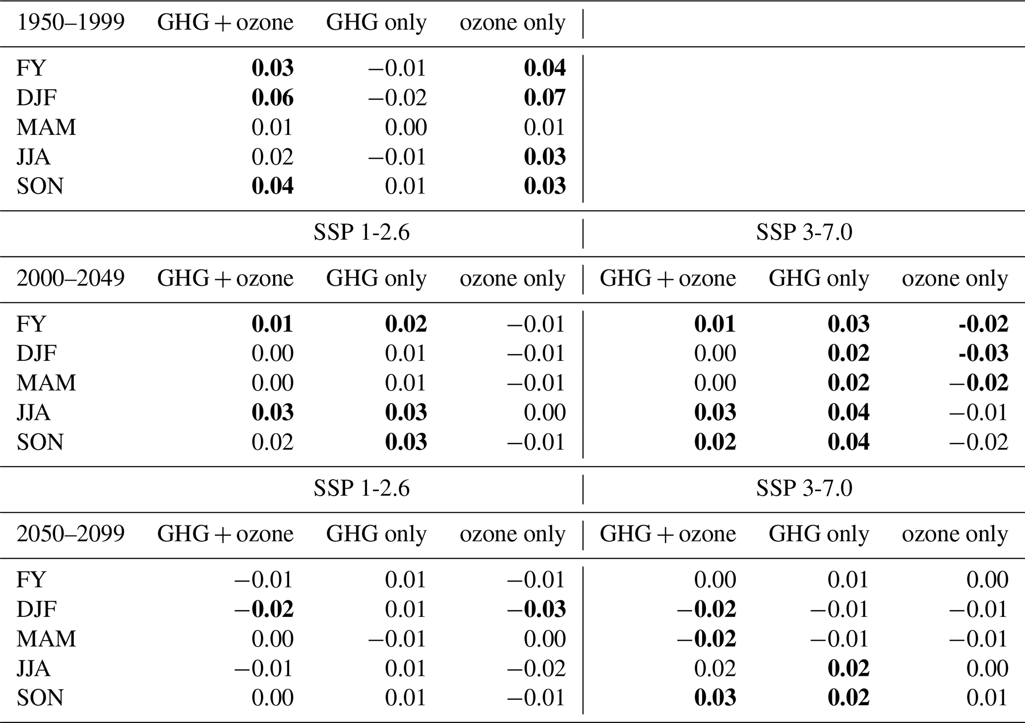
In the first half of the 21st century (2000–2049), in the realistic (ODS-HIST) runs, winds stay approximately constant in most seasons in both SSP scenarios, though they increase substantially in austral winter (Table 6). This lack of trend is due to the (accelerating) GHG effect countering the (decelerating) ozone recovery effect, which can be seen when decomposing the overall signal into the two forcing factors (Table 6). Though the acceleration due to GHG is stronger under the higher-emissions (SSP 3-7.0) scenario, the effect of ozone recovery is also stronger under this scenario and the two effects cancel out (Table 6). The sensitivity of ozone recovery to SSP pathway reflects the interaction of other GHGs (e.g. CH₄ and N₂O) with ozone chemistry. SSP 3-7.0 has higher CH₄ concentrations in the future than SSP 1-2.6, and UKESM1 has a significant ozone response to increasing CH₄ (see Fig. 14 in Zeng et al., 2022). Ozone recovery will therefore be accelerated in SSP 3-7.0 relative to SSP 1-2.6, with a concomitant stronger forcing of surface winds. The overall acceleration seen in austral winter (JJA) is a result of the different seasonalities of the two forcing factors: while ozone depletion and recovery is predominantly a summer phenomenon, these simulations show that GHG-driven wind increase is strongest in winter, resulting in an unbalanced GHG forcing of wind trends during austral winter. Using a regression analysis of CMIP6 simulations, Morgenstern (2021) finds a similar seasonality in CO₂ forcing of the SAM. Simpkins and Karpechko (2012) also see this strong winter increase in the SAM, which is related to the winds, also concluding that the difference is due to the lack of ozone recovery in winter.

Finally, in the latter half of the 21st century (2050–2099), the simulations show a difference in wind trends based on GHG emission level. Under SSP 1-2.6 with historical ozone recovery, wind speed stagnates in all seasons, while under SSP 3-7.0, winds accelerate in austral winter and spring, both with and without ozone depletion (Fig. 7). However, these trends are typically not statistically significant, due to large interannual variability. Analogous results were found by Simpkins and Karpechko (2012), who noted the dependence of SAM trends on emissions scenario and also noted the lack of statistical significance.

4 Discussion and Conclusions

The main aims of this work were to evaluate the representation of recent-past Southern Ocean winds in the most commonly used contemporary reanalysis products, in a free-running Earth system model (UKESM1) and other CMIP6 models with interactive ozone, and finally to use UKESM1 to attribute the drivers of changes in winds over the recent past and through to 2100. The initial intercomparison of the reanalyses shows that, while the general features of the Southern Ocean winds (mean, distribution, jet location, and extremes) are relatively congruent, the reanalyses vary considerably in wind speed trends. In all reanalyses, trends are strongest in the period of maximum ozone depletion (1980–1999), and comparatively strongest in austral summer, consistent with the existing understanding of surface wind forcing by ozone loss, which is primarily a summer phenomenon. However, trends in MERRA2 are comparatively much stronger and tend to persist year-round, while trends in ERA5 and JRA3Q are weaker and concentrated in austral summer.

We assess which trend representation is more realistic using a novel observational constraint: we compare trends in the observational SAM index to their representation in the reanalyses, and then relate them to wind speed trends. Because a positive (negative) SAM index trend is mechanistically linked to a positive (negative) wind trend, performance in one metric can provide information about performance in the other. Applying this constraint suggests the large winter trends seen in winter and spring in the MERRA2 reanalysis may be spurious, as they are accompanied by strong SAM trends not seen in the observational record. Spuriously large trends in the previously commonly used NCEP-NCAR reanalysis were also observed by Morgenstern (2021); here we suggest that this problem persists in MERRA2. Thus, we conclude that ERA5 and JRA3Q are best suited for studies of wind and SAM changes in this region, as well as for forcing ocean models.

UKESM1 winds and SAM index evaluate well against our baseline reanalysis (ERA5). Notably, UKESM1 performs well in reproducing the intensity distribution of daily wind speeds seen in ERA5, including the high wind speed tail of the distribution, though the overall mean of the distribution is somewhat higher in UKESM1 (∼ 0.3 m s⁻¹). UKESM1 also reproduces the ERA5 historical decadal trends in both wind speed and the SAM index, including the differential response between the 1980–2000 period and the full 40 year period, indicating a realistic sensitivity of winds to ozone changes. The seasonality of the SAM and wind speed trends is also well reproduced, with strongest trends in austral summer. However, the poleward progression of the jet latitude is stronger in UKESM1 than in any of the reanalyses, somewhat in contrast to the correctly reproduced behaviour of the other metrics.

We find that UKESM1 represents wind trends well relative to similar CMIP6 models with interactive chemistry (Sect. 3.3), but highlight again that the accurate wind speed trends in UKESM1 are realized in combination with too strong ozone decline, particularly in the period 1980–1990. We note that the relationship between TCO depletion and wind trends in the CMIP6 models holds only partially in austral summer. No relationship is observable in austral winter, consistent with the understood low role of ozone in forcing wind changes in this season.

Using future projections made with UKESM1, with and without ozone depletion, we attribute the observed changes to the relative influence of ozone depletion and greenhouse gas emissions, both historically over 1980–2020 and as projected by the model to the end of the 21st century. The UKESM1 simulations show the observed acceleration of winds in the latter half of the 20th century is entirely attributable to ozone depletion. In the first half of the 21st century, summer winds stagnate, as the decrease of wind speeds due to ozone recovery competes with wind speed increase due to GHG emissions. In contrast, wind speeds increase in austral winter and spring, as the GHG effect outcompetes the ozone recovery effect, which is predominantly a summer phenomenon. In the latter half of the 21st century, a more clear bifurcation between wind speed trends under the low and high SSP scenario is visible, especially in austral winter and spring. Winds accelerate more under the high SSP scenario, while stagnating under the low SSP scenario. In this time period, the role of ozone recovery is minor.

We show that ozone depletion overwhelmingly drove the observed summer wind acceleration in the latter half of the 20th century, and we expect this trend to reverse in the first half of the 21st century. By the second half of the 21st century, greenhouse gas loading is the main factor driving wind changes, with more emissions leading to more acceleration, but it is strongly active only in austral winter and spring. Thus, we demonstrate a shift in the dynamical controls on the wind behaviour over the Southern Ocean from ozone in the latter half of the 20th century to greenhouse gas emissions in the latter half of the 21st century.

This control shift is consistent with the general understanding. As in Barnes et al. (2014), we find historical wind speed trends due to ozone depletion are stronger than greenhouse gas driven trends seen in the twenty first century. Similar to Barnes et al (2014)., Gerber and Son (2014.), McLandress et al. (2011), and Simpkins and Karpechko (2012), we observe a cancellation of effects in the first half of the twenty first century, as ozone recovery competes with greenhouse gas emissions, leading to only weak wind trends in this period. We also reproduce the dependence of future trends on greenhouse gas emission strength seen in Simpkins and Karpechko (2012) and other studies. Our work, focusing on near-surface winds, extends this understanding by providing an estimate of the changing wind trends in response to the shift in dominant forcing. We do this using an Earth system model (UKESM1), with full-atmosphere interactive chemistry, allowing a large set of interactions and feedbacks to be simulated; chemically between a range of GHGs and stratospheric ozone, between both sets of gases and atmospheric dynamics, and between the atmosphere and the underlying ocean and sea ice. The ability of UKESM1 to represent these interactions, and how they shape surface winds over the Southern Ocean, was validated against both reanalyses and an observational SAM index and further contextualized against other CMIP6 models with interactive ozone chemistry. Our analysis suggests UKESM1 is suitable for investigating links between ozone loss and recovery, GHG scenarios, and Southern Ocean uptake of heat and carbon.