Critical freshwater forcing for AMOC tipping in climate models – compensation matters

Ocean and climate models of various complexity have shown that the Atlantic Meridional Overturning Circulation (AMOC) can undergo tipping, i.e., transition abruptly to a state without North Atlantic deep-water formation, as a function of freshwater forcing. Most of these model experiments compensate for the freshwater input to conserve global salinity, with salt being added either at the surface or throughout the ocean volume. However, these two different compensation methods have so far only been compared in a single, coarse-resolution climate model, and therefore little is known robustly about the effect of salinity compensation on the AMOC tipping point. Here, using an ocean model at 1° resolution and an intermediate-complexity coupled climate model, we systematically compare the effect of surface vs. volume compensation on the tipping point of the AMOC as diagnosed from quasi-equilibrium experiments using a freshwater flux over the region 20–50° N. Salinity compensation at the surface consistently delays AMOC tipping compared to volume compensation. This is mainly because the compensation salinity added over the subpolar North Atlantic counteracts the weakening salinity gradient from freshwater forcing. In contrast to an earlier study, the compensation method does not introduce qualitative differences in AMOC recovery when tracing the full hysteresis loop. In light of these results, volume compensation appears to provide the best trade-off between global salinity conservation and similarity to the effects of a physical freshwater flux. Our results indicate that the distance of present-day climate to the AMOC tipping point with respect to freshwater forcing might have been overestimated in recent modeling studies, compounding the effect of model biases.

1 Introduction

The Atlantic Meridional Overturning Circulation (AMOC) shapes the Earth's present-day climate through its northward transport of heat, carbon and nutrients. Climate model simulations and paleoclimate evidence suggest that the AMOC can not only operate in the present-day “On” state but also in a qualitatively different “Off” state, in which deep water formation in the North Atlantic would cease (Broecker et al., 1985; Rahmstorf, 2002; Boers et al., 2022; Loriani et al., 2025). An abrupt transition (tipping) from the “On” to the “Off” state would have global climate implications, including Northern Hemisphere cooling (e.g., Vellinga and Wood, 2002; Jackson et al., 2015; Liu et al., 2017), a shift in monsoon patterns (e.g., Ben-Yami et al., 2024) and a reduction in ocean carbon uptake (e.g., Schaumann and Alastrué de Asenjo, 2025). It is an open question whether the AMOC could reach a critical threshold in the 21st century or beyond (Fox-Kemper et al., 2021; Dijkstra and van Westen, 2026), but due to the substantial impacts associated with such an event, it is of high importance to understand the associated mechanisms.

Most conceptual and climate modeling studies have probed AMOC stability and tipping with respect to freshwater input into the North Atlantic (Weijer et al., 2019). The idea first proposed in a two-dimensional box model (Stommel, 1961) is that, in a certain parameter range of freshwater forcing, the AMOC can have two competing stable states, with the “On” state losing stability beyond a critical forcing threshold. By slowly ramping the freshwater forcing parameter up and down in “quasi-equilibrium”, it is possible to trace the AMOC hysteresis loop (Rahmstorf et al., 2005) and identify the critical forcing parameter or tipping point. This approach has been successfully applied across the hierarchy of ocean and climate models, from conceptual models (see review by Dijkstra, 2024), Earth System Models of Intermediate Complexity (e.g., Schmittner et al., 2002; Rahmstorf et al., 2005; Willeit and Ganopolski, 2024) and global ocean models (e.g., Rahmstorf, 1995; Prange et al., 2003; van Westen et al., 2025) to atmosphere–ocean general circulation models (GCMs; Hawkins et al., 2011; Hu et al., 2012; van Westen and Dijkstra, 2023).

The use of a single, scalar forcing parameter necessitates the choice of a region of freshwater input, whose effect was first studied by Rahmstorf (1996), and a strategy to conserve global salinity (Jackson et al., 2017). Some modeling studies (e.g., Rahmstorf et al., 2005) did not prescribe any salinity compensation, and instead allowed the global ocean to gradually freshen when ramping up the freshwater forcing. However, on timescales of centuries to millennia, global salinity is usually seen as a fixed integral condition determined by the continental ice sheet configuration (e.g., Kageyama et al., 2017). In addition, without salinity conservation, the quasi-equilibrium approach cannot demonstrate multistability, as the “On”- and “Off”-states for the same freshwater forcing value would have different global salinities. To keep the global salinity constant, quasi-equilibrium experiments compensate for the freshwater input regionally or globally at the surface (“surface compensation”; Rahmstorf, 1996; Gregory et al., 2003; Hawkins et al., 2011; van Westen et al., 2024b), or through the entire ocean volume (“volume compensation”; Jackson et al., 2017, 2023). Surface compensation is sometimes framed as freshwater flux anomalies being induced by changes in the hydrological cycle (e.g., Hogg et al., 2013), while volume compensation can be motivated as a trade-off between mimicking a net freshwater input (e.g., from land ice) while keeping global salinity as a fixed integral condition (Jackson et al., 2023).

While the sensitivity to different surface compensation regions has been reported qualitatively in several (coarse-resolution) models (Rahmstorf and Ganopolski, 1999; Dijkstra and van Westen, 2024), only one study has so far systematically compared the effects of global surface compensation vs. volume compensation: using the coarse-resolution climate model FAMOUS, Jackson et al. (2017) found that the difference between the compensation methods was mainly in the AMOC recovery due to qualitatively different “Off” states. However, the impact of the compensation strategy on the position of the AMOC tipping point at which the “On”-state loses stability has so far remained inconclusive. In addition, it is not known how well the strong differences in hysteresis generalize to other models.

In this study, we systematically assess the influence of surface vs. volume compensation on the critical freshwater forcing values of the AMOC in two global climate models – an ocean model at 1° resolution and an intermediate-complexity climate model. This allows probing the dependence of the AMOC tipping point on the compensation strategy, with implications for the interpretation of previous quasi-equilibrium hosing studies.

2 Materials and Methods

2.1 Models

The very high computational cost of the quasi-equilibrium approach precludes the exploration of different methodological choices with state-of-the-art (CMIP-class) coupled climate models. Because both resolution and atmosphere–ocean coupling (Jackson et al., 2017) have previously been shown to be important for AMOC tipping and hysteresis, we use two different models in this study: a standalone ocean model at 1° resolution, i.e., at the same ocean resolution as state-of-the-art coupled climate models, and a coupled climate model of intermediate complexity, which can capture large-scale atmospheric feedbacks on the AMOC.

The standalone ocean model is version 2α of the Parallel Ocean Program (POP; Dukowicz and Smith, 1994) at a horizontal resolution of 1° and 40 vertical levels with a layer spacing between 10 m near the surface and 250 m in the deep ocean. The model uses a dipole grid (“gx1v6”) with the North Pole centered over Greenland, such that the local resolution reaches about 50 km in the Labrador Sea. Here, we use the same model configuration as the “x1” configuration of Weijer et al. (2012) and refer to their supplementary material for a detailed description and validation. Surface boundary conditions are provided by standard bulk formulae (Large and Yeager, 2004) and correspond to the monthly averaged normal-year forcing of Large and Yeager (2004), which represents average 1958–2000 climatic conditions. The model was spun up for 2000 years and shows no significant drift in the AMOC strength under fixed normal-year forcing. It does not include interactive sea ice but applies temperature and salinity restoring with a timescale of 30 d under a prescribed seasonal sea ice extent, which mimics sea ice freshwater fluxes. No salinity restoring is applied elsewhere.

The intermediate-complexity climate model is version 1.4.0 of Climber-X (Willeit et al., 2022). In the configuration used here, it consists of dynamic ocean, atmosphere, sea-ice, and land components at a horizontal resolution of 5°×5°. The ocean component is the frictional-geostrophic ocean model GOLDSTEIN (Edwards et al., 1998; Edwards and Marsh, 2005) using 23 vertical layers with a spacing between 10 m near the surface and 200 m in the deep ocean. Calculating horizontal velocities from the frictional-geostrophic balance generally leads to dampening of strong currents such as the Antarctic Circumpolar Current and the Gulf Stream (Edwards and Marsh, 2005; Müller et al., 2006), but otherwise the ocean mean state compares favorably to observations (Willeit et al., 2022). The atmospheric component SESAM (Willeit et al., 2022) can be classified as 2.5-dimensional, as prognostic variables are only horizontally resolved, but empirical information about their vertical structure is taken into account for heat and moisture transport and for longwave radiation. The sea ice model SISIM includes both thermodynamics, based on the zero-layer model of Semtner (1976), and dynamics, using an elastic-viscous-plastic rheology (Hunke and Dukowicz, 1997; Bouillon et al., 2009). We refer to Willeit et al. (2022) for a comprehensive model description and evaluation against present-day observations.

Both models have different strengths and shortcomings. POP has a much higher resolution than Climber-X but simulates a slightly too strong AMOC mean state (21.5 Sv under normal-year forcing) compared to present-day observations of around 17 Sv (Johns et al., 2023) and has a positively biased freshwater transport at 34° S in the South Atlantic (F_ovS≈0.2 Sv compared to −0.15±0.09 Sv in observations; Arumí-Planas et al., 2024). However, these biases are correlated in climate models and POP lies well within the range of CMIP6 models (van Westen and Dijkstra, 2024). In addition, they are only expected to shift the AMOC tipping point quantitatively (van Westen et al., 2025) and should not influence our results in a qualitative way. Climber-X, while featuring a rather diffusive AMOC due to its low resolution, has an AMOC strength (19.4 Sv) and an F_ovS value (−0.10 Sv) closer to observations, in addition to sea ice and a (simplified) atmosphere coupling. We believe that the diversity of both approaches implies robustness for results corroborated by both models.

2.2 Experimental design

Here, we follow the quasi-equilibrium hosing approach used most recently by van Westen and Dijkstra (2023). Each model is initialized from an equilibrated (present-day or pre-industrial) state and freshwater forcing is ramped up at a rate of 0.3 Sv kyr⁻¹, for which it has been shown that the AMOC remains relatively close to its (quasi-)equilibrium strength (Vanderborght et al., 2025). This forcing is applied over a time-period of 1500 years, corresponding to a final value of 0.45 Sv. By this point, all simulations have reached an “AMOC off”-state. The freshwater forcing is then decreased at the same rate until the AMOC recovers, and the hysteresis loop can be closed by ramping up the forcing again until it reaches zero.

In this study, the freshwater forcing is applied uniformly between 20–50° N in the North Atlantic. This ensures consistency with previous quasi-equilibrium experiments in different climate models which used the same hosing region (Rahmstorf et al., 2005; Hawkins et al., 2011; Hu et al., 2012; van Westen and Dijkstra, 2023) and is motivated by not forcing the regions of deep-water formation directly, but instead inducing an AMOC collapse through large-scale feedbacks (cf. Weijer et al., 2019; Vanderborght et al., 2025). The hosing is applied as a virtual salt flux (Jackson et al., 2023), for which the surface salinity tendency is given as:

$$\begin{array}{}\text{(1)}& {{\displaystyle \frac{\mathrm{d}{S}_{\mathrm{0}}}{\mathrm{d}t}}}_{\text{hos}}=\mathrm{-}{\displaystyle \frac{{\mathit{\varphi }}_{\text{hos}}{S}_{\mathrm{0}}}{\mathrm{\Delta }{z}_{\mathrm{0}}}},\end{array}$$

where ϕ_hos is the hosing freshwater flux per unit area (in m s⁻¹), S₀ is the surface salinity and Δz₀ is the depth of the upper layer. Note that POP uses a fixed reference salinity of 35 g kg⁻¹ instead of the surface salinity (as in Climber-X) on the right-hand side of Eq. (1).

We compare two different salinity compensation strategies to ensure conservation of global salinity: surface compensation (“S-comp” hereafter) and volume compensation (“V-comp” hereafter). In the surface-compensated case, a salt flux of opposite sign is added uniformly over the entire ocean surface (excluding the hosing region) such that the total surface salt flux from hosing and compensation add up to zero. This yields:

$$\begin{array}{}\text{(2)}& {\mathit{\varphi }}_{\text{comp}}=-{\displaystyle \frac{A_{\text{hos}}}{A-A_{\text{hos}}}}{\mathit{\varphi }}_{\text{hos}},\end{array}$$

where A_hos is the area of the hosing region and A is the global ocean surface area.

In the volume-compensated case, the compensation salinity is distributed over the entire ocean volume (including the hosing region) and calculated as Jackson et al. (2023)

$$\begin{array}{}\text{(3)}& {{\displaystyle \frac{\mathrm{d}S}{\mathrm{d}t}}}_{\text{comp}}=F_{\text{tot}}/V,\end{array}$$

where V is the global ocean volume and

$$\begin{array}{}\text{(4)}& F_{\text{tot}}=\int {\mathit{\varphi }}_{\text{hos}}{S}_{\mathrm{0}}\mathrm{d}x\mathrm{d}y,\end{array}$$

is the total salt input at any timestep.

2.3 Reconstruction of AMOC changes

To attribute changes in AMOC strength, the AMOC is reconstructed using the thermal wind balance relation, which relates the AMOC strength to the density – and therefore temperature and salinity – gradient within the Atlantic basin. We follow the methodology of Vanderborght et al. (2025), which has successfully been applied to the quasi-equilibrium AMOC collapse in the Community Earth System Model (CESM), which uses POP as its ocean model component. We start out from the relation

$$\begin{array}{}\text{(5)}& {\displaystyle \frac{{\partial }^{\mathrm{2}}\widehat{\mathrm{\Psi }}(z,t)}{\partial z^{\mathrm{2}}}}={\displaystyle \frac{gC}{{\mathit{\rho }}_{\mathrm{0}}f}}{\mathrm{\Delta }}_y\mathit{\rho }(z,t)\end{array}$$

Butler et al. (2016), where $\widehat{\mathrm{\Psi }}$ is the reconstructed interior streamfunction maximum between 0 and 30° N, Δ_yρ is the meridional density gradient, g=9.81 m s⁻¹ is the gravitational acceleration, ρ₀=1026 kg m⁻³ is the seawater density, and $f={\mathrm{10}}^{-\mathrm{4}}$ is the Coriolis parameter at northern mid-latitudes.

In theory, the AMOC is associated with a zonal, rather than meridional, pressure gradient. The proportionality between these two gradients is encoded in the non-dimensional constant C through CΔ_yρ=Δ_xρ, with Δ_xρ representing the zonal density difference (e.g., Marotzke, 1997). The precise origin of this proportionality remains poorly understood, with earlier studies highlighting the importance of eastern-boundary dynamics, where stratification anomalies radiate into the interior via propagating Rossby waves (Gnanadesikan, 1999; Pedlosky and Spall, 2005; Cessi and Wolfe, 2009; Schloesser et al., 2012; Vanderborght and Dijkstra, 2025). Schloesser et al. (2014) derived an expression for C in a simplified overturning model. Although this derivation has not yet been generalised, the relation expressed in Eq. (5) captures real, but still incompletely understood, physics and has been broadly validated across studies that successfully reproduce the AMOC response under variable forcing conditions (e.g., de Boer et al., 2010; Haskins et al., 2019; Bonan et al., 2022; Nayak et al., 2024; Bonan et al., 2025; Vanderborght et al., 2025), providing confidence in our approach. The value C=0.85 used here is motivated in Appendix A.

Equation (5) is integrated with the boundary conditions $\widehat{\mathrm{\Psi }}\left(\mathrm{0}\right)=\widehat{\mathrm{\Psi }}\left(z_b\right)=\mathrm{0}$, where z_b=4750 m is the lower boundary of the North Atlantic Deep Water cell in the initial state. The density gradient Δ_yρ in the Atlantic is calculated between two boxes spanning 20° S to the equator for the southern box and 43–65° N for the northern box (see Appendix A).

When diagnosing the AMOC directly from the model velocities, we refer to the AMOC index as the maximum of the Atlantic overturning streamfunction between the equator and 30° N.

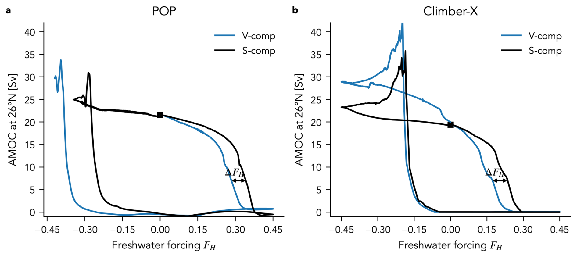
Figure 1 Hysteresis loop obtained from quasi-equilibrium experiments with a forcing rate of 0.3 Sv kyr⁻¹ for (a) POP and (b) Climber-X. Black lines show the cases with surface compensation and blue lines with volume compensation, and squares indicate the initial AMOC state. ΔF_H is the difference between critical forcing values (here approximated as the point where the AMOC reaches 7 Sv).

3 Results

3.1 AMOC hysteresis

The quasi-equilibrium freshwater forcing triggers abrupt AMOC changes and a wide hysteresis in both POP and Climber-X (Fig. 1). In both models, the AMOC “On”-state initially weakens more strongly with volume compensation (V-comp) than with surface compensation (S-comp). Because the AMOC strength at the tipping point is similar between compensation cases, this implies that the AMOC tipping point is crossed for lower freshwater forcing values with volume compensation. The difference ΔF_H between critical freshwater forcing values (S-comp minus V-comp) is very similar in both models, around 0.06 Sv (Fig. 1). In Climber-X, the quasi-equilibrium experiment was repeated at a six-fold slower rate of 0.05 Sv kyr⁻¹ (as in Rahmstorf et al., 2005), at which the difference between critical forcing values becomes slightly smaller (0.04 Sv) but remains robust qualitatively (Fig. B1).

Before investigating the mechanisms of the lower critical freshwater forcing in V-comp compared to S-comp in detail, we briefly focus on the “Off”-state and the AMOC recovery. In the S-comp case in both POP and Climber-X (Figs. 2 and B2), the overturning circulation develops a strong reverse cell with deep convection in the Southern Ocean immediately after the AMOC collapse (cf. van Westen et al., 2025), resembling the “southern sinking” states of Marotzke and Willebrand (1991) and Huisman et al. (2009). In V-comp, the “Off”-state initially does not feature this reverse cell, and generally no deep overturning cell in any of the basins (Figs. 2 and B2). Interestingly, this resembles the “Off”-state in van Westen et al. (2024b), although they used surface compensation. In both models used here, this state appears to be transient: by the time the “Off”-branch of the V-comp hysteresis has reached 0 Sv, the “Off”-state also shows the strong reverse cell. In contrast to Jackson et al. (2017), none of the four simulations show an active Pacific Meridional Overturning Circulation (PMOC) at any point in the hysteresis (Figs. 2 and B2).

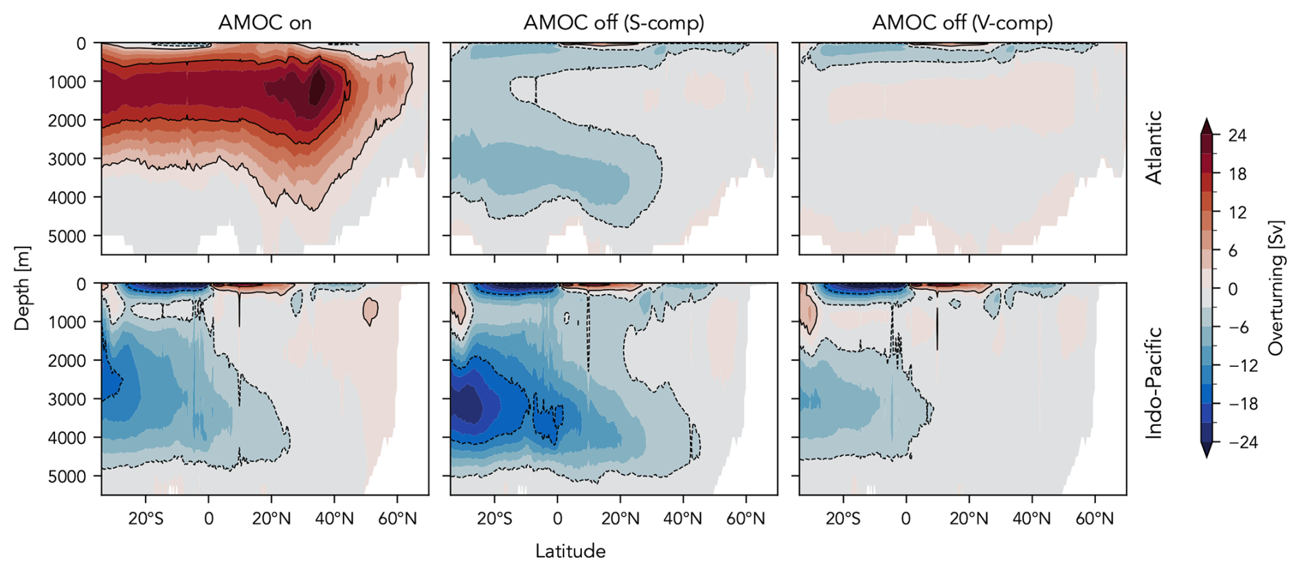
Figure 2 Overturning streamfunction of the AMOC “On” and AMOC “Off”-states in POP. First row: Atlantic, second row: Indo-Pacific. The AMOC “On” state is the initial state indicated by the black marker in Fig. 1a. The AMOC “Off” states are averaged over the last 100 years ($F_H\in [\mathrm{0.42},\mathrm{0.45}]$ Sv) of the ramp-up simulations. See Fig. B2 for the streamfunctions in Climber-X.

In both models, the simulation with volume compensation recovers from the “Off”-state later (i.e., for lower freshwater forcing values) than with surface compensation. In Climber-X, this difference is small and can be attributed to the rate of freshwater forcing; at the slower rate of 0.05 Sv kyr⁻¹, both compensation cases recover at the same forcing value, which is also larger compared to the recovery at a fast rate (Fig. B1). In POP, the difference in recovery between S-comp and V-comp is much larger than in Climber-X (by around 0.2 Sv) and therefore unlikely to be only an effect of the forcing rate. One possible explanation is that Southern Ocean surface freshwater forcing is capable of triggering an AMOC recovery from the AMOC “Off”-state as previously demonstrated by Weaver et al. (2003), and the surface compensation becomes a freshwater forcing outside the North Atlantic for hosing values smaller than zero. However, we consider this issue outside the scope of this paper and focus on the differences in loss of stability of the “On”-state in the following.

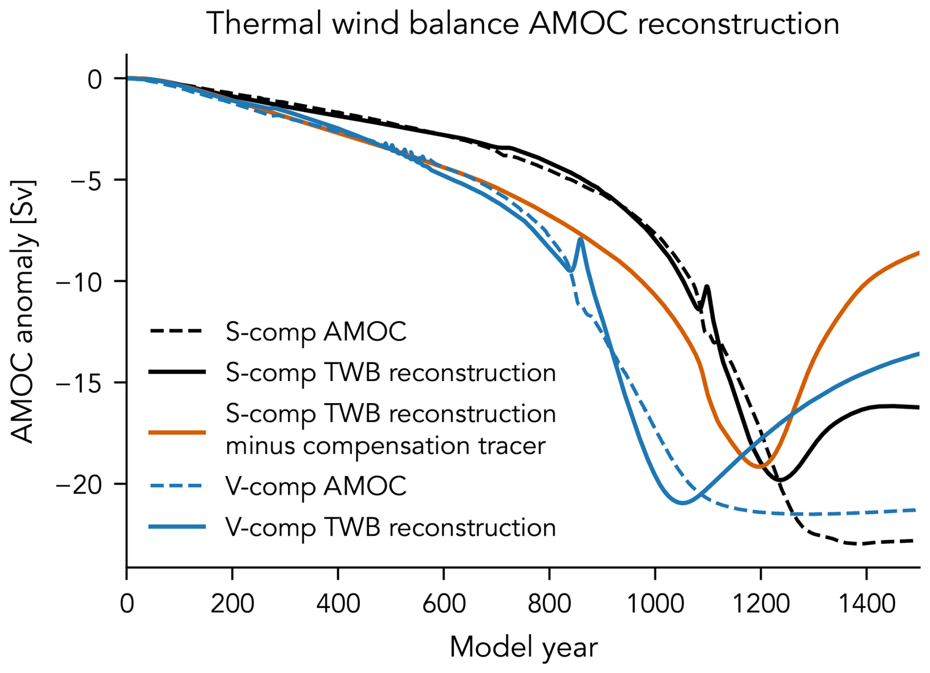
Figure 3 AMOC anomalies in POP (compared to the initial state) diagnosed directly from model velocities (dashed lines) compared to the AMOC reconstruction $\widehat{\mathrm{\Psi }}$ from the thermal wind balance relation of Eq. (5). The orange line shows the reconstruction repeated after subtracting the compensation salt tracer and applying a linear temperature feedback term (see text for details).

3.2 Attribution of changes in AMOC strength before the tipping point

In POP, in both S-comp and V-comp, the AMOC anomalies on the “On”-branch can be faithfully reconstructed from the meridional density gradient Δ_yρ using the thermal wind balance framework introduced in Sect. 2.3. The resulting timeseries at a depth of 1000 m are shown in Fig. 3. The reconstruction matches the original AMOC timeseries only up to the tipping point, after which the structure of the overturning changes fundamentally (cf. Fig. 2). Because of this and the fact that tipping in S-comp and V-comp occurs at a similar AMOC strength, we focus on attributing the differences in the initial AMOC weakening (until model year 800) in the following.

To this end, the AMOC weakening is decomposed into a temperature and a salinity component, as well as into density changes in the northern and in the southern box. Temperature and salinity contributions are diagnosed by re-calculating Δ_yρ while keeping salinity and temperature, respectively, at their initial values. Similarly, the northern and southern contributions are diagnosed by keeping the southern and northern density fixed, respectively.

The results of this decomposition are shown in Fig. 4a, demonstrating that the AMOC weakening in the quasi-equilibrium experiment is mostly driven by salinity and by changes in the North Atlantic. As in Vanderborght et al. (2025), the negative salinity contribution ${\widehat{\mathrm{\Psi }}}_{\mathrm{S}}$ is opposed by a positive temperature contribution ${\widehat{\mathrm{\Psi }}}_{\mathrm{T}}$. These two contributions are almost perfectly linearly proportional (${\widehat{\mathrm{\Psi }}}_{\mathrm{T}}=-\mathrm{0.814}{\widehat{\mathrm{\Psi }}}_{\mathrm{S}}$, r²=0.9995), such that we can treat the temperature contribution as a linear feedback term below. As expected, changes in the North Atlantic dominate the density gradient changes as well as the salinity contribution, with a small, opposite contribution from the South Atlantic.

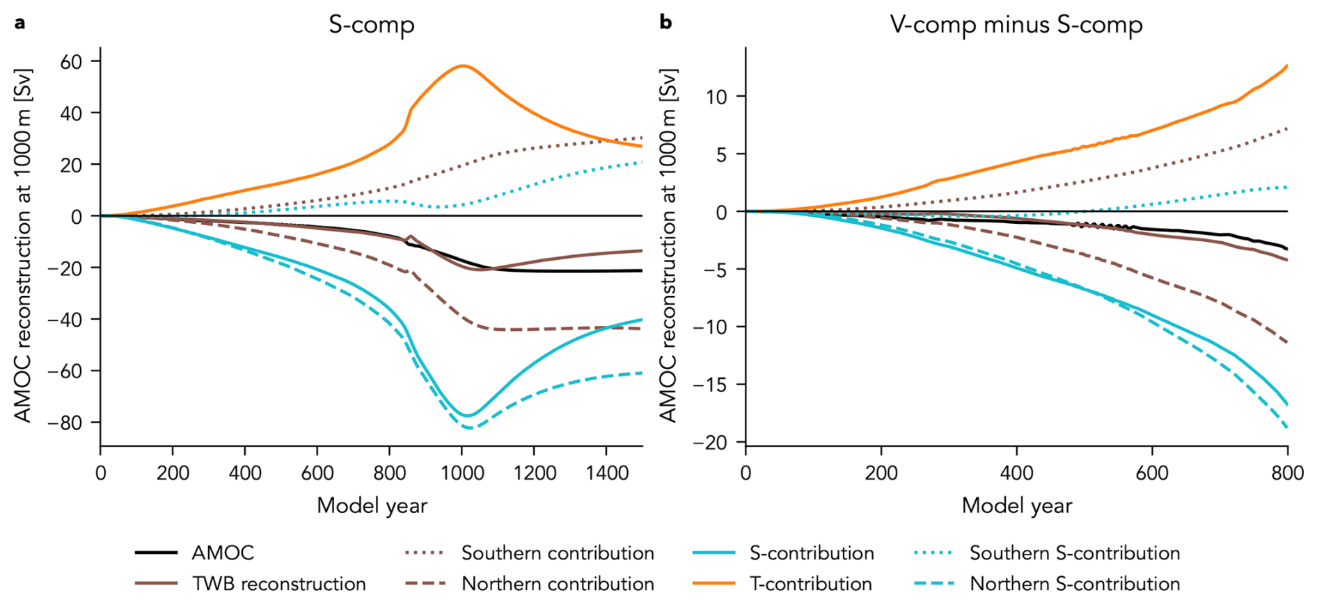
Figure 4 Decomposition of the reconstructed AMOC anomalies in POP: (a) decomposition of AMOC anomalies in S-comp into contributions from temperature and salinity changes as well as density changes in the North and South Atlantic, (b) difference between V-comp and S-comp for each of the components. Note that only model years 1 to 800 are shown here.

A similar picture emerges for the differences between S-comp and V-comp (Fig. 4b). The additional weakening in V-comp can be attributed to salinity changes, with an opposing contribution from temperature changes. This salinity contribution can be almost entirely attributed to the North Atlantic, with salinity changes in the South Atlantic contributing slightly to the additional weakening in the first 400 years, before changing sign and slightly opposing the additional weakening. However, when including the temperature component, South Atlantic changes once again are a small but opposing contribution to the additional AMOC weakening throughout.

3.3 Fate and impacts of compensation salinity

Having established that the differences in AMOC weakening between S-comp and V-comp are mainly due to salinity differences in the North Atlantic, we now diagnose the origin of these salinity differences in more detail. For this purpose, we included a passive tracer for the compensation salinity in the S-comp simulation in POP. The passive tracer follows the same model physics as the prognostic salinity. It is set to zero everywhere initially and is subject to the same virtual salt flux ϕ_comp at the surface where salinity compensation is added. This allows tracing the fate of the surface compensation salinity in a physically consistent way.

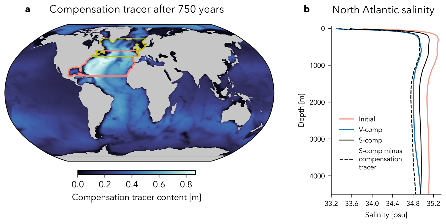
Figure 5 Fate of the compensation salinity in the POP S-comp simulation after 750 years (freshwater forcing F_H=0.225 Sv): (a) Vertically integrated concentration of the compensation salinity tracer; the hosing region is indicated by the orange box. (b) Salinity profiles in the North Atlantic box (43–65° N, yellow box in panel a). The initial salinity profile and the profile in V-comp are shown for comparison, and the total salinity minus the compensation tracer is shown as a dashed line.

The geographical distribution of the surface salinity tracer in POP after 750 years is shown in Fig. 5a. Somewhat surprisingly, the highest concentrations of compensation salinity can be found in the hosing region (20–50° N), the only region where no compensation salinity is added at the surface, and in the subpolar gyre just north of the hosing region. Relatively high concentrations can also be found in the South Atlantic and in the Arctic Ocean, while the Indo-Pacific shows lower concentrations, suggesting a strong leakage of the compensation salinity from the Indo-Pacific into the Atlantic. A similar picture emerges in Climber-X (Fig. B3a), except that there is more storage of compensation salinity in the Arctic Ocean in S-comp compared to POP. Climber-X also allowed testing the fate of the compensation salinity in V-comp (Fig. B3b). In strong contrast to S-comp, the compensation tracer remains distributed almost uniformly across the world ocean.

The impact of surface compensation on the North Atlantic salinity profile, which we identified as decisive for the less strong AMOC weakening in S-comp compared to V-comp in POP, can be clearly seen in Fig. 5b. Due to the freshwater input and AMOC weakening, there is a negative salinity anomaly throughout the water column in both S-comp and V-comp compared to the initial state. However, the anomaly is only about half as strong in S-comp as in V-comp. This can be almost entirely attributed to the added salt from surface compensation: when subtracting the surface compensation tracer in S-comp, the salinity profile matches that of V-comp well, especially in the upper 1000 m.

We can now quantify the impact of the (northern) compensation salinity on the AMOC weakening in S-comp via the thermal wind balance relation. To this end, we subtract the compensation salinity tracer from the prognostic salinity for POP and re-calculate Δ_yρ and $\widehat{\mathrm{\Psi }}$ using this modified salinity. The AMOC anomaly obtained this way is only physically meaningful when accounting for the temperature feedback, which we treat as a linear term by multiplying the result with the temperature feedback factor derived above. The resulting AMOC anomaly without the influence of compensation salinity is shown as orange line in Fig. 3. It matches the AMOC weakening in V-comp very well until around year 600, regardless of whether the procedure is applied to the entire Atlantic or only to the northern box (not shown). This means that the initial difference in AMOC weakening between S-comp and V-comp is directly determined by the effect of surface compensation salinity, which counteracts the freshening in the North Atlantic. Only after year 600, additional feedbacks appear to become important in V-comp.

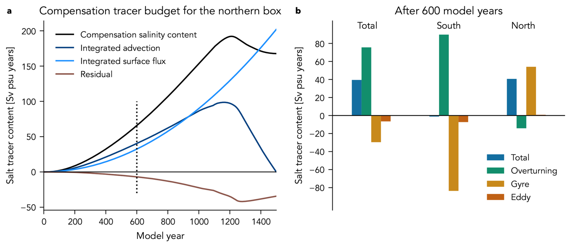
Figure 6 Integrated budget of the salinity compensation tracer in POP S-comp for the North Atlantic between approximately 43 and 65° N. (a) Time series of tracer content, time-integrated advective and surface tracer fluxes, and a residual calculated as the difference between these three components. The budget includes the (parametrized) eddy contribution, such that the small but non-negligible residual is probably due other parametrizations not included in the model output, such as horizontal diffusion. (b) Integrated contributions to the advection component, after subtracting the barotropic component, after 600 years (dotted line in panel a).

If the compensation salinity in the North Atlantic determines the first-order differences between S-comp and V-comp, where does it originate from? In S-comp, there are only three possible pathways: transport from the South or from the North, or input at the surface. These components, as well as the tendency $\mathrm{d}{S}_{\text{comp}}/\mathrm{d}t$, are calculated offline from monthly POP output and their integrated (cumulative) contributions to the compensation salt content in the North Atlantic (43 to 65° N) are shown in Fig. 6a.

For most of the AMOC weakening phase before the tipping point, the surface flux directly over the region and the advective transports both contribute about half to the accumulation of compensation salinity. The advective contributions are further detailed (after 600 years, but the results do not change qualitatively for other years before the tipping point) in Fig. 6b. Because the overturning and gyre components almost entirely compensate at the southern boundary of the region, the net inflow of the compensation tracer is determined by the inflow from the North. The northern inflow can be mostly attributed to the azonal (gyre) transport, with a small, opposing contribution from the overturning transport.

3.4 Effect of different compensation regions

To obtain a more detailed estimate of the importance of different surface compensation regions on the AMOC tipping point, we conduct a series of sensitivity experiments with Climber-X. In these experiments, different regions (defined in Fig. 7) are removed one-by-one from the surface compensation mask. To provide an “apples-to-apples” comparison, the remaining compensation salinity is instead distributed throughout the global ocean volume, such that the unit compensation salinity flux per surface area is the same across all simulations. This way, we can assess the influence of individual regions on the progressive AMOC destabilization when switching from surface to volume compensation.

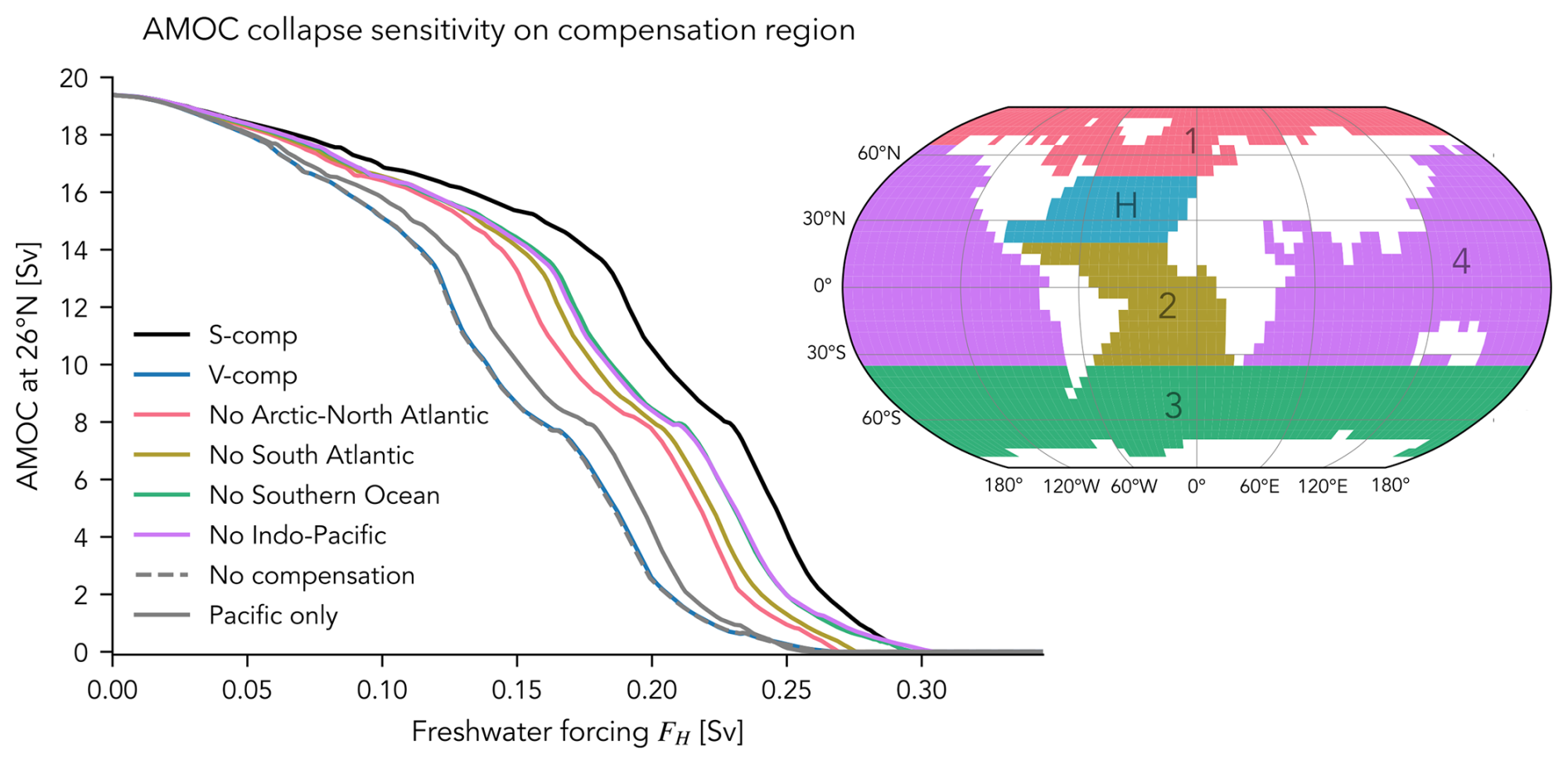
Figure 7 AMOC collapse in Climber-X with a forcing rate of 0.3 Sv kyr⁻¹ when removing different regions from the surface compensation mask. Regions are shown in the map inset: 1 = Arctic-North Atlantic, 2 = South Atlantic, 3 = Southern Ocean, 4 = Indo-Pacific. The hosing region is marked with an “H”. The additional compensation cases are shown in grey: “No compensation” does not apply any compensation salinity (i.e., the global salinity changes) and “Pacific only” applies all surface compensation over the Pacific (with no additional volume compensation).

Figure 7 shows that the AMOC tipping point of each of these simulations lies between S-comp and V-comp. Removing the Indo-Pacific or Southern Ocean from the surface compensation mask has a moderate impact on the AMOC tipping point, with the freshwater forcing threshold decreasing by around 30 % compared to the difference in thresholds between S-comp and V-comp (Table 1). The change in thresholds is around 40 % for the South Atlantic and more than half for the North Atlantic and the Arctic Ocean combined. This is consistent with the analysis of POP above, in that adding salinity within the Atlantic basin is the main cause for the differences in the AMOC tipping point between S-comp and V-comp.

Table 1 Differences between the AMOC tipping points in Fig. 7. ΔF_H(Exp)= difference in critical freshwater forcing values (here defined as where the AMOC reaches 7 Sv) between this experiment (“Exp”) and S-comp; $\mathrm{\Delta }{F}_H\left(\text{Exp}\right)/\mathrm{\Delta }{F}_H\left(\text{V-comp}\right)=$ same as the previous column, but divided by the difference between V-comp and S-comp; Normalized by area = same as normalized difference, but additionally divided by the area ratio between the masked-out region and the global surface compensation area.

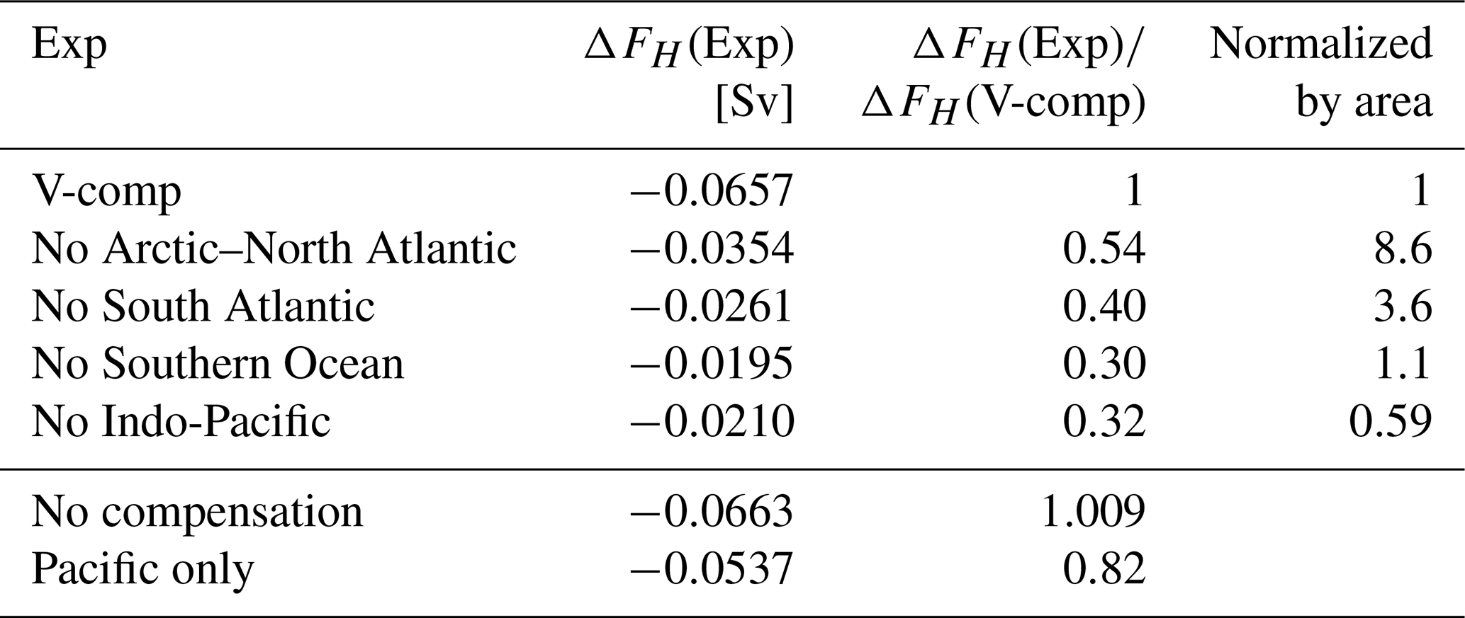
The area (and therefore the total salt input) of these regions differs widely, such that the impact of the different regions can be more equally compared when normalizing the change in critical thresholds by each region's surface area (Table 1). This is done by dividing the percentage effect by the area of each region, such that an index of 1 is equal to the globally averaged effect of surface compensation. According to this metric, surface compensation in the North Atlantic and Arctic has an 8-times stronger influence on the AMOC tipping point than the global average surface compensation. This factor is still larger than 3 for the South Atlantic but only around 0.6 for the Indo-Pacific. The Southern Ocean has an influence that is comparable to the global average. The regional effects do not entirely add up linearly, so that these numbers should be interpreted qualitatively rather than quantitatively, but they clearly show that surface compensation added over the North Atlantic has an outsized role in shaping the differences between S-comp and V-comp, with an important role also for the South Atlantic.

On the other hand, the relatively small role of the (Indo-)Pacific motivates revisiting alternative surface compensation strategies; for example, Dijkstra and van Westen (2024) and Rahmstorf and Ganopolski (1999) have previously applied the surface compensation term over the Pacific instead of globally. In agreement with our previous analysis, in this “Pacific only” case (grey solid line in Fig. 7), the AMOC tips for only slightly higher freshwater forcing values (around 18 % of the difference between V-comp and S-comp) than the volume-compensated case.

Finally, we performed a simulation without any salinity compensation (dashed grey line in Fig. 7), in which the global salinity is allowed to gradually freshen, keeping in mind that this “no compensation” case is not suitable to demonstrate a multi-stable AMOC regime. The AMOC collapse trajectory is extremely similar to that of V-comp, with a negligible difference (less than 1 % of the difference between S-comp and V-comp) of the critical AMOC threshold. This justifies the use of volume compensation when assessing the effect of a physical freshwater flux on the AMOC tipping point.

The results in this section raise the question whether using an effective surface freshwater flux parameter $F_H^{\text{eff}}$ would make V-comp and S-comp more comparable in forcing space. Indeed, when defining $F_H^{\text{eff}}$ as the net surface freshwater forcing (from hosing and surface compensation) over the entire Atlantic and Arctic basins, S-comp and V-comp match very well in POP and at least become closer in Climber-X (Fig. B4). While this is only a very approximate indicator, it may be helpful for future inter-model comparison if different compensation strategies had been used.

4 Discussion and Conclusions

In this study, we showed that the method of salinity compensation matters when estimating critical freshwater forcing values for AMOC tipping from climate models. In two different modeling setups, the AMOC tipping point consistently shifted to higher freshwater forcing values with surface compensation compared to volume compensation. The thermal wind balance AMOC reconstruction as well as targeted sensitivity experiments showed that the most important cause of the differences between the two configurations is the input and accumulation of surface compensation salinity north of the hosing region, i.e., in the deep-water formation regions of the North Atlantic.

We can now compare our results with those of Jackson et al. (2017), who performed a similar comparison between S-comp and V-comp with the coarse-resolution ($\approx \mathrm{5}\mathit{°}\times \mathrm{5}\mathit{°}$) atmosphere–ocean GCM FAMOUS. In agreement with both models used here, they also found a stronger initial AMOC weakening in V-comp compared to S-comp. Based on the analysis of the prognostic salinity and velocity fields, they concluded that this additional weakening was due to the salt input at the surface in S-comp, a result that we could now rigorously demonstrate with the use of a diagnostic surface compensation tracer. The FAMOUS results (cf. their Fig. 6a) are therefore consistent with an AMOC tipping point shifted to later values in S-comp, underlining the robustness of our main conclusion.

The main differences with Jackson et al. (2017) lie in the recovery of the AMOC from the “Off”-state. The hysteresis in FAMOUS was much wider in S-comp than in V-comp owing to the formation of a vigorous Pacific Meridional Overturning Circulation (PMOC) during the AMOC collapse in the S-comp, stabilizing the “AMOC off” state. In contrast, no PMOC forms in any of our four model simulations, and consequently there is only a quantitative but no qualitative difference in hysteresis between the two compensation cases. As pointed out by Jackson et al. (2017), one possible explanation for PMOC formation in their model (and the absence of a PMOC here) is that FAMOUS has a subsurface salinity maximum in the North Pacific which is not seen in observations. In contrast, the North Pacific salinity and density profiles in POP and Climber-X, and therefore stratification, are in fairly good agreement with observations (Fig. B5). However, FAMOUS is actually biased toward a too strong (and not too weak) upper-ocean stratification in the North Pacific (Fig. B5d), i.e., a larger “barrier” to overcome to form a PMOC. Hence, it remains for further study which model differences facilitate PMOC formation, especially since Baker et al. (2025) proposed a link between AMOC weakening and strengthening of the Pacific overturning under global warming.

The main trade-off of our relatively expensive experimental design is the use of simplified modeling approaches, which come with several caveats. For POP, these are mainly the absence of interactive atmosphere and sea ice components. It was shown by van Westen et al. (2024a) that sea ice feedbacks mainly affect the physics of the “Off”-state and AMOC recovery; however, we do not expect that it would affect the difference between S-comp and V-comp in a qualitative way. Climber-X includes both a sea-ice and a (simplified) atmospheric component, but the ocean model has a coarse resolution and only includes quasi-geostrophic dynamics. Nevertheless, in the spirit of the model hierarchy (Held, 2005), our different but complimentary approaches, combined with the results of Jackson et al. (2017), demonstrate that the main result that the AMOC collapses for lower freshwater forcing in V-comp compared to S-comp is robust.

A final caveat for both models (and all coupled models which have run quasi-equilibrium hosing experiments so far) is that, due to their resolution, they parametrize the effects of mesoscale eddies. Using an idealized eddy-permitting ($\mathrm{1}/\mathrm{4}\mathit{°}$) model, Hogg et al. (2013) found that the AMOC weakened more with surface compensation compared to no compensation when applying a strong freshwater input of 0.5 Sv over the North Atlantic for 400 years. They attributed this difference mainly to stronger Southern Ocean upwelling in the “no compensation” (their FW2) case. However, it is unclear whether this means that the effect of surface compensation would actually be different in a high-resolution global model, or whether the differences arise due to the idealized setup in Hogg et al. (2013), especially the use of a rectangular single-basin geometry and a linear equation of state.

Quasi-equilibrium experiments with climate models have so far mostly used surface compensation (Hawkins et al., 2011; Hu et al., 2012; van Westen et al., 2024b), while volume compensation has been used in the recent North Atlantic Hosing model intercomparison project (Jackson et al., 2023). There may be good reasons to use surface compensation, for example to enable direct comparison with previous quasi-equilibrium simulations or potentially faster convergence to a new equilibrium. However, we showed that surface compensation, especially applied over the North Atlantic and the Arctic Ocean, has non-negligible unintended side effects. It has previously been shown that surface compensation can also affect the climate response to AMOC weakening (Stocker et al., 2007), an aspect that would be worth revisiting in future work. It is worth noting that there is little physical justification to apply a positive salinity flux term over the mid- and high-latitudes, as the intensification of the hydrological cycle under global warming will increase (and not decrease) P−E there (Held and Soden, 2006).

On the other hand, volume compensation affects the AMOC behavior very little compared to a physical freshwater input with no compensation (Fig. 7), e.g., from ice sheet mass loss. When volume compensation cannot be used for technical or scientific reasons, surface compensation over the Pacific can be a pragmatic compromise that limits artificial stabilization of the AMOC. In any case, the choice of salinity compensation should always be explicitly documented; otherwise, future comparisons of different modeling studies will be complicated further.

To conclude, this study demonstrated a robust mechanism why the critical freshwater forcing threshold for the “AMOC on” state shifts to higher values when using global surface compensation compared to volume compensation. If this result indeed translates to more complex coupled climate models, this would mean that critical thresholds estimated from quasi-equilibrium simulations (e.g., van Westen et al., 2024b) would have been overestimated. This could compound the effect of model biases such as a salinity bias in the Indian Ocean, which is also expected to bias the critical freshwater forcing towards higher values (Dijkstra and van Westen, 2024; Boot and Dijkstra, 2025).

Appendix A: AMOC reconstruction using thermal wind balance

The thermal wind balance reconstruction of the AMOC from Eq. (5) has three free parameters: the boundaries of the northern and southern boxes, and the proportionality constant C. Here, we outline how these were chosen for POP.

The northern box is fixed at 43–65° N in the Atlantic following Vanderborght et al. (2025), consistent with the region of outcropping isopycnals that overlap with the Southern Ocean (Fig. A1). However, probably because the densest waters in the North Atlantic do not reach the Southern Hemisphere (Fig. A1a), the reconstruction following Eq. (5) does not agree well with the actual AMOC strength if the southern box is chosen in the Southern Ocean as in the coupled CESM (Vanderborght et al., 2025). Good agreement could only be achieved if different values of C were chosen for S-comp and V-comp, for which there is no physical justification.

Instead, in line with the initial Atlantic density structure (Fig. A1), we choose the southern box inside the South Atlantic at 20° S–0° N. The parameter C=0.85 is chosen such that the reconstructed AMOC strength in the initial state agrees well with the modeled AMOC, with the reconstructed AMOC decline matching the actual decline well during the first 800 years (i.e., before reaching the tipping point) for both S-comp and V-comp. This leads to a good agreement of the simulated and reconstructed AMOC changes, which are the focus of this study, for both configurations.

We tested that our conclusions remain robust to changes in the definition of the southern box, namely by repeating the analysis in Sect. 3.2 with the southern box definitions of Bonan et al. (2025) (30° S–30° N) and Vanderborght et al. (2025) (56–34° S, 53° W–20° E) with C=1.1 and C=0.6, respectively. In both cases, the northern salinity contribution remains the dominant component in Fig. 4 (not shown), with a slightly larger opposing contribution from the southern box using the definition of Bonan et al. (2025).

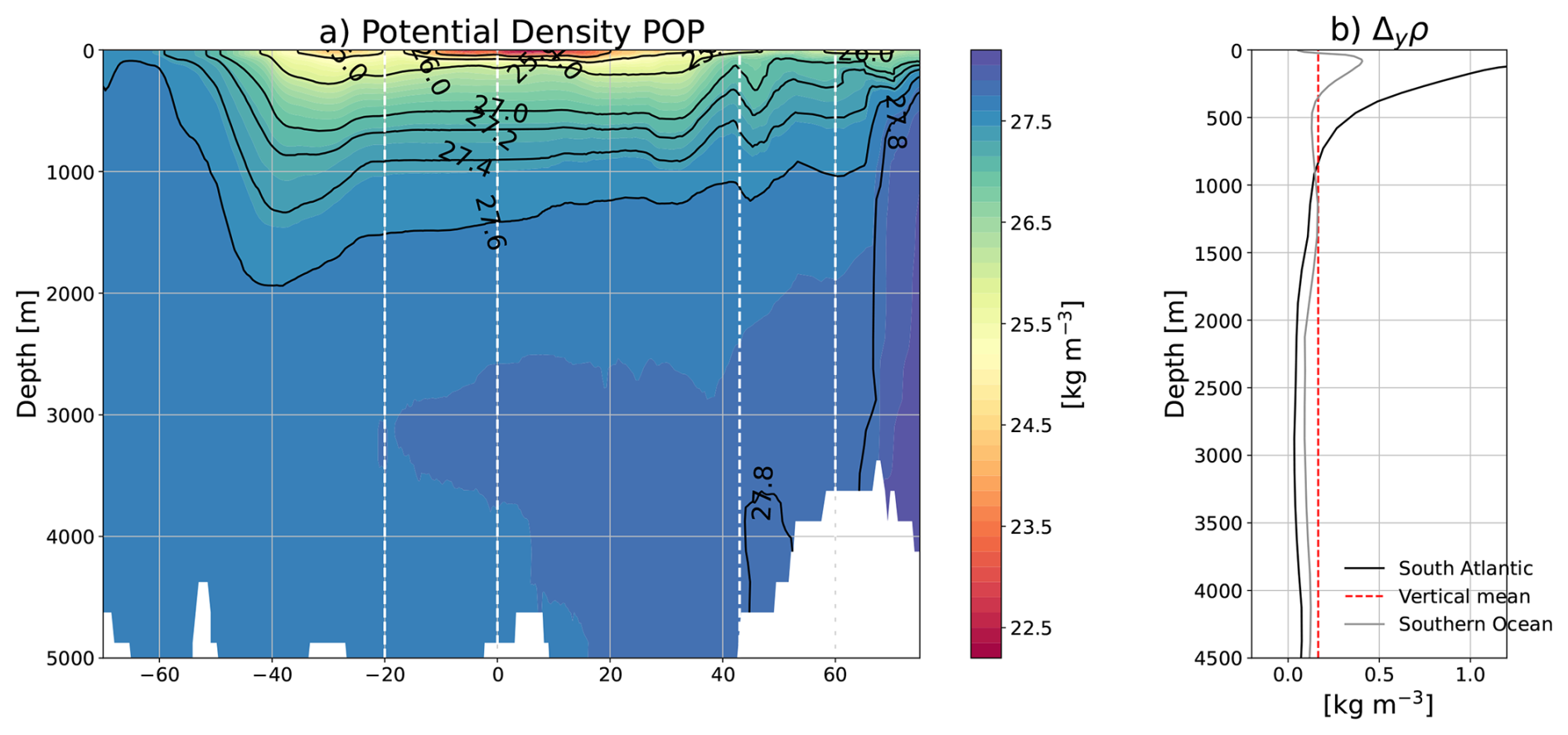
Figure A1 (a) Zonal mean potential density (σ₀) in the Atlantic and in the Southern Ocean (south of 34° S, zonal extent 53° W to 20° E) for the initial state of POP. (b) Potential density gradient Δ_yρ using two possible choices of the southern box: 20° S to the equator (“South Atlantic”, used in the main text) and 56 to 34° S (“Southern Ocean”, as in Vanderborght et al., 2025). The vertical mean is shown for the “South Atantic” box.

Appendix B: Supplementary figures

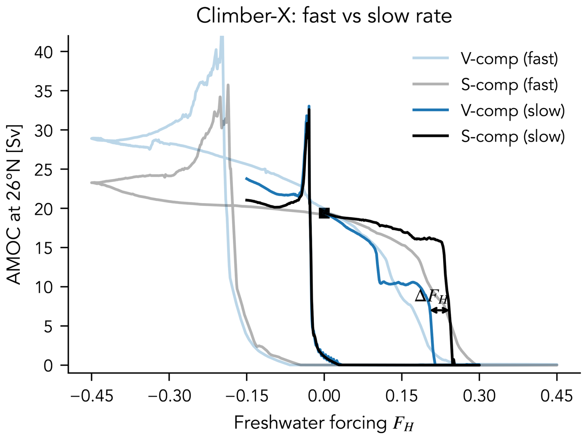
Figure B1 Comparison of AMOC hysteresis in Climber-X at two different rates: 0.3 Sv kyr⁻¹ (“fast”; same as in POP) and 0.05 Sv kyr⁻¹ (“slow”). ΔF_H marks the difference in critical thresholds (as in Fig. 1) in the slow hysteresis. The “plateau” in the V-comp case appears to be an intermediate stable state resembling the stable “weak AMOC” state of Willeit and Ganopolski (2024).

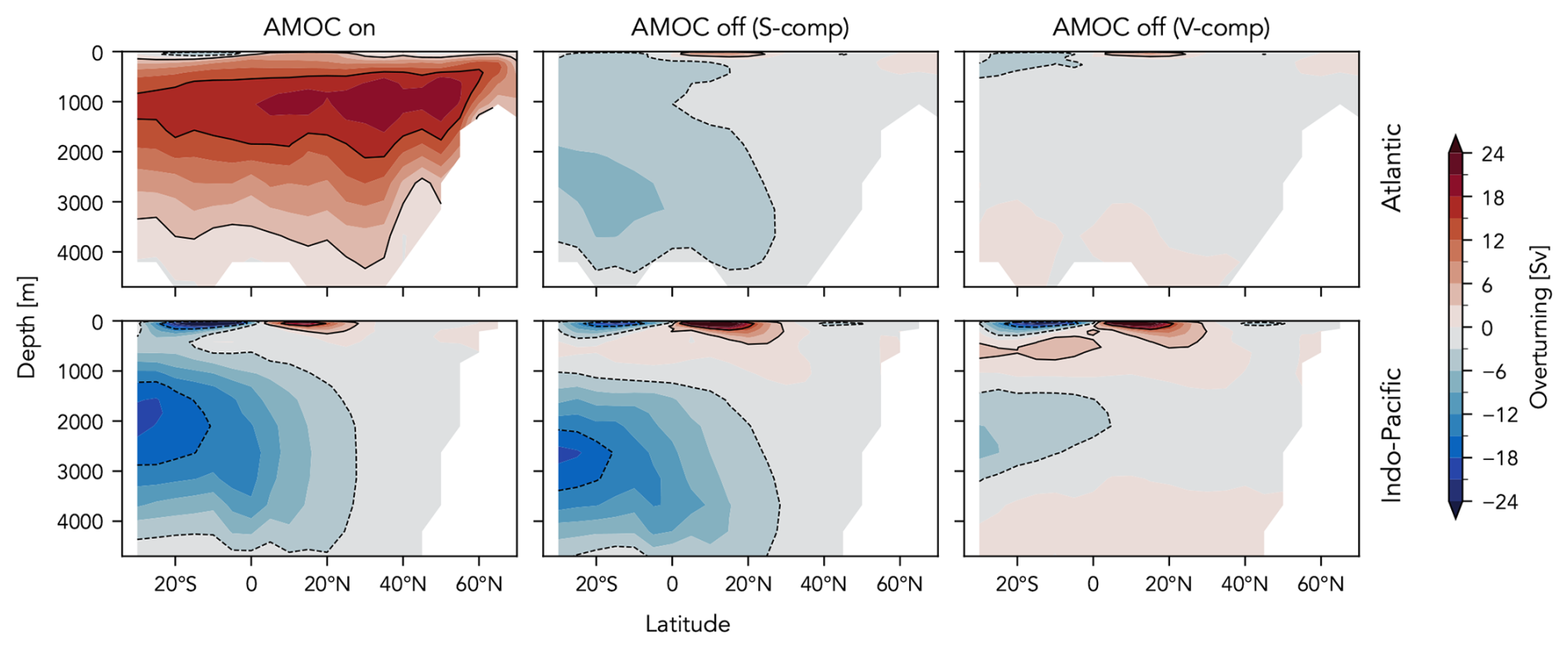
Figure B2 Overturning streamfunction of the AMOC “On” and AMOC “Off”-states in the Climber-X hysteresis. First row: Atlantic, second row: Indo-Pacific. The AMOC “On” state is averaged over the first 100 years and the AMOC “Off” states are averaged over the last 100 years of the ramp-up simulations.

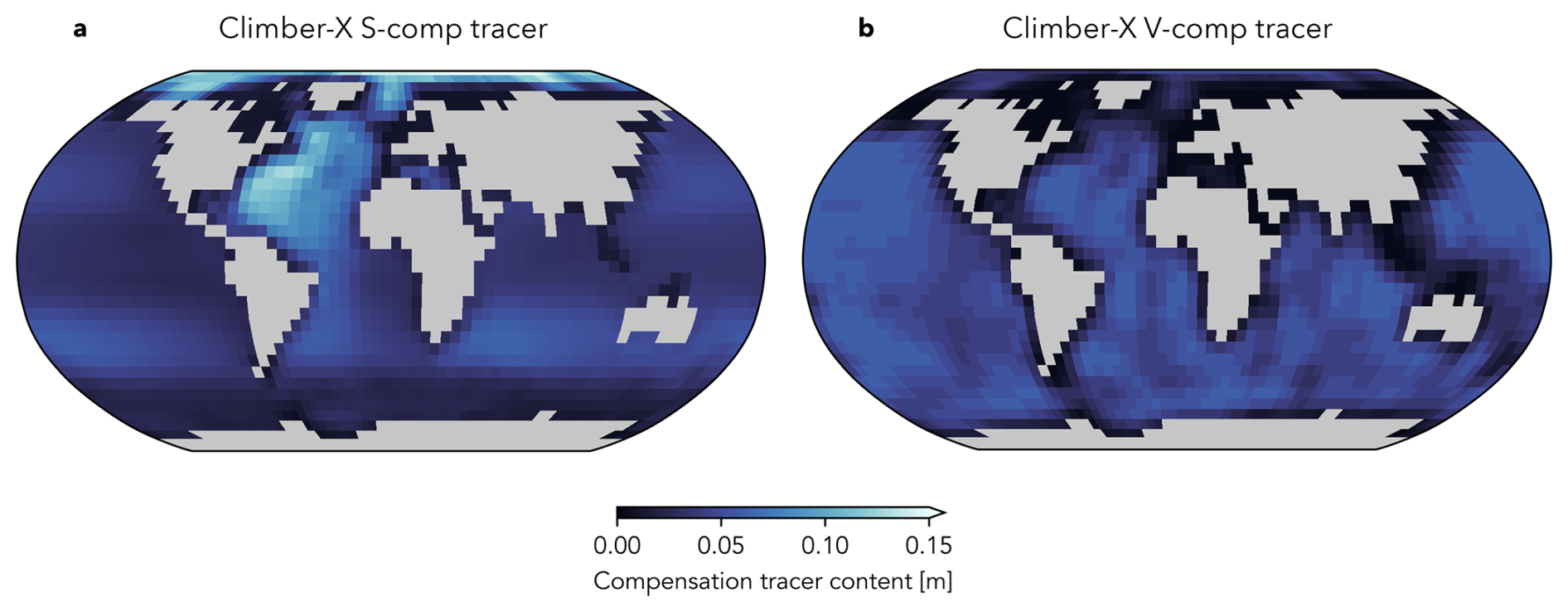
Figure B3 Fate of the compensation salinity in Climber-X after 300 years (before the tipping point in any of the simulations): (a) S-comp, (b) V-comp.

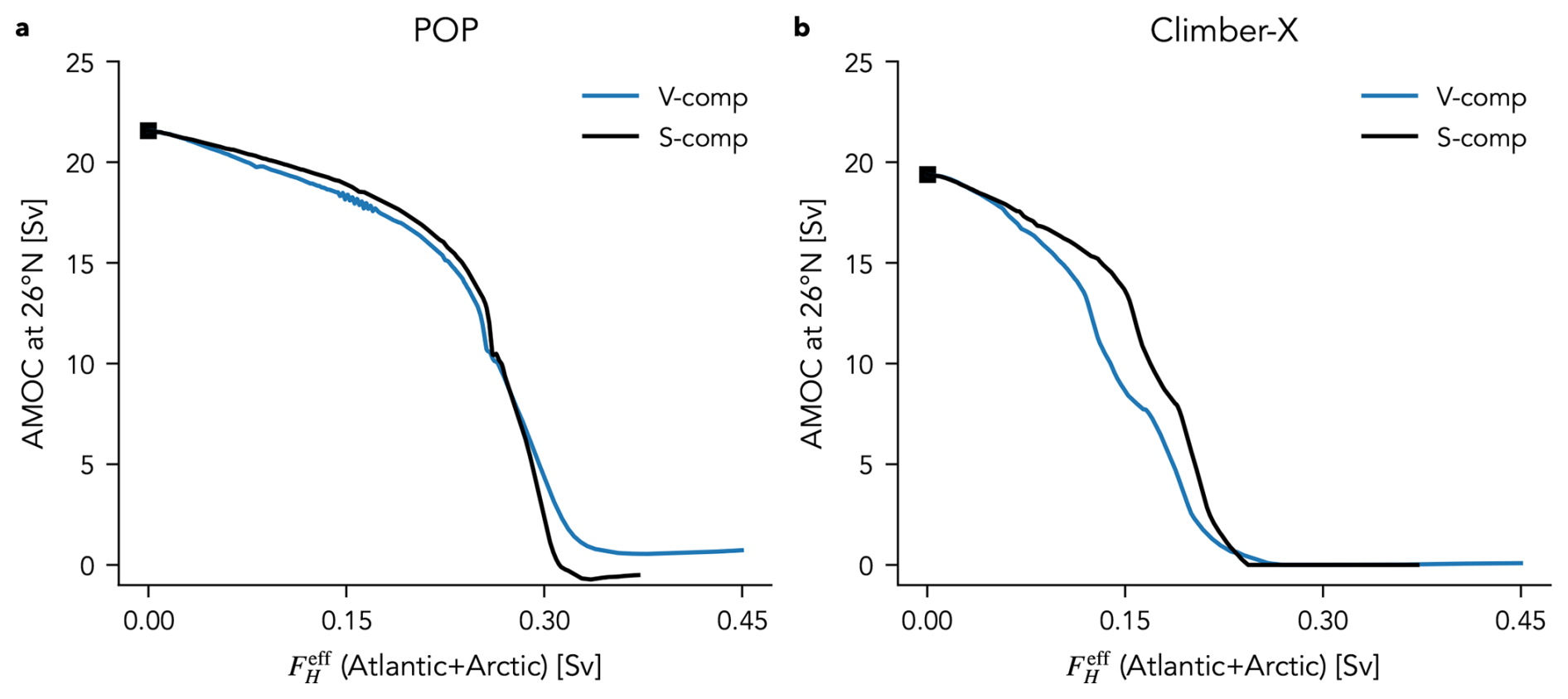
Figure B4 Forward branch of the hysteresis curves from Fig. 1 against effective freshwater forcing $F_H^{\text{eff}}$ over the entire Atlantic and Arctic basins.

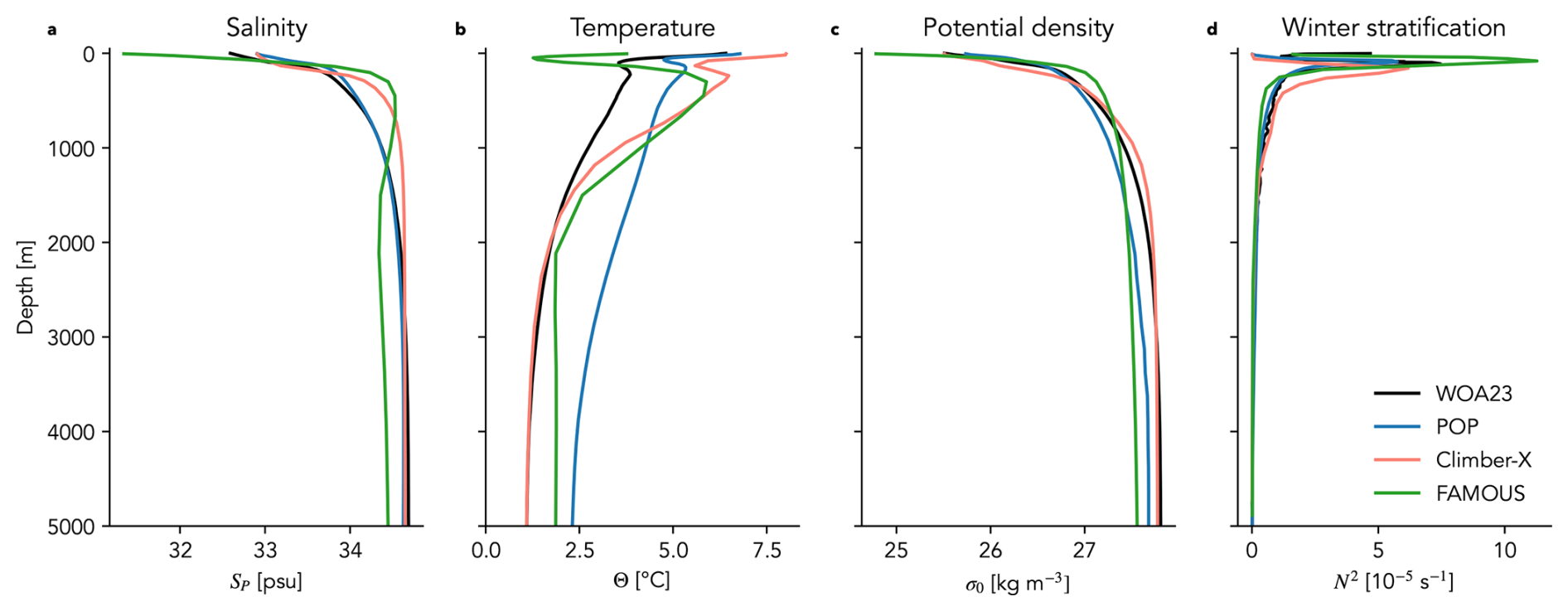
Figure B5 Model evaluation against observations for the North Pacific (north of 45° N). Observations are the 1970–2000 climatology from the World Ocean Atlas 2023 (WOA23; Locarnini et al., 2024; Reagan et al., 2024) and the FAMOUS climatology is the pre-industrial state from version XDBUA (Smith et al., 2008), which is very similar to the initial state in Jackson et al. (2017). (a) Salinity, (b) potential temperature, (c) potential density, (d) stratification ($N^{\mathrm{2}}=-g/{\mathit{\rho }}_{\mathrm{0}}\partial \mathit{\rho }/\partial z$). All quantities are annual means except for stratification, which is averaged over the winter months (December to March).