Detecting transitions and quantifying differences in two SST datasets using spatial permutation entropy

Weather prediction systems rely on the vast amounts of data continuously generated by Earth modeling and monitoring systems, and efficient data analysis techniques are needed to track changes and compare datasets. Here we show that a nonlinear quantifier, the spatial permutation entropy (SPE), is useful to characterize spatio-temporal complex data, allowing detailed analysis at different scales. Specifically, we use SPE to analyze ERA5 and NOAA OI v2 sea surface temperature (SST) anomalies in two key regions, Niño 3.4 and Gulf Stream. We perform a quantitative comparison of these two SST products and find that SPE detects differences at short spatial scales (<1°). We also identify several transitions, including a transition that occurs in 2007 when ERA5 changed its sea–surface boundary condition to OSTIA, in 2013 when OSTIA updated the background error covariances, and in 2021 when NOAA SST changed satellite, from MeteOp-A to MeteOp-C. The robustness and statistical significance of the detected transitions are tested using surrogate data. We demonstrate that, using standard distance and cross-correlation analyses, the transitions are not detected with the same level of statistical significance and robustness as when using ordinal analysis.

1 Introduction

Due to the large amount of data generated by Earth modeling and monitoring systems, much effort is currently being devoted to developing new, efficient climate data analysis techniques (Dijkstra et al., 2019; Messori et al., 2017; Boers et al., 2019; Gupta et al., 2021; Díaz et al., 2023; Krouma et al., 2024; Allen et al., 2025). Ordinal analysis (Bandt and Pompe, 2002) is a popular symbolic method of time-series analysis that has been applied to geophysical data. For example, ordinal analysis was used to study time series of surface air temperature anomalies in a regular grid over the earth's surface (reanalysis data from the National Center for Environmental Prediction/National Center for Atmospheric Research NCEP/NCAR) and uncovered long-range tele-connections across multiple time scales (Barreiro et al., 2011; Deza et al., 2013). The ordinal method is based on estimating the probabilities of symbols, known as ordinal patterns (OPs), defined in terms of the temporal order of the relative values of L data points. As an example, for L=3, triplets of consecutive data values such that $x_t<x_{t+\mathrm{1}}<x_{t+\mathrm{2}}$ are encoded in the symbol “012” where the digits represent the rank of the corresponding value within the triplet. The symbols' probabilities are estimated from their frequencies of occurrence within the time series and their Shannon entropy, known as permutation entropy (PE), is a quantifier of nonlinear temporal correlations. PE is low when some OPs are much more probable than others, and maximum when all possible OPs are equally probable (Bandt and Pompe, 2002). Ordinal analysis is computationally very efficient and robust to the presence of artifacts and noise. The use of time-lagged (non-consecutive) data points adds versatility to the method, since it allows to select different temporal scales for the analysis. For example, for analyzing a climatic time series with monthly resolution, the L=3 OPs can be defined by considering data values in three consecutive months (e.g. January, February, March; February, March, April; etc), in three consecutive years, or equally spaced over a period of time (for example, a year) (Deza et al., 2013). An important limitation of the ordinal methodology is that the symbolic coding rule does not take into account the actual values of the data points, but their relative values, and therefore, ordinal analysis gives partial information, complementary to that obtained by using standard time series analysis techniques.

Ordinal analysis was originally proposed for time series analysis and adapted for the analysis of gridded two-dimensional spatial data (Ribeiro et al., 2012), by defining the OPs in terms of the relative values of L grid points. Spatial ordinal analysis is a versatile tool because one can choose different “shapes” and/or different spatial orientations for the symbols. For example, for symbols defined in terms of the data values of L=4 grid points, one can consider squares of 2×2 grid points, a line (horizontal or vertical) of 4 grid points, an “L” composed by 3+1 grid points, etc. Furthermore, the use of spatially lagged grid points allows tuning the spatial scale of the analysis. This spatial lag is an important parameter for the application of this analysis tool in climate science, as the dynamics of our climate involves complex processes and interactions that act at different spatial scales. Ordinal analysis has also been expanded to include more information from the analyzed signals, such as the variance of the data points that define an OP (Fadlallah et al., 2013), their amplitude (Azami and Escudero, 2016), or the dispersion of data points that define different OPs (Politi, 2017). However, ordinal analysis is one of many symbolic techniques available, and in addition to permutation entropy other entropy quantifiers for time series can also provide valuable information (Prado et al., 2020; Falasca et al., 2020; Ikuyajolu et al., 2021; Novi et al., 2024; Paluš et al., 2024).

The spatial permutation entropy (SPE), which is Shannon's entropy estimated from the probabilities of spatial ordinal patterns, has been used to analyze images, art works and textures (Sigaki et al., 2018, 2019; Tirabassi and Masoller, 2023; Tirabassi et al., 2023; Muñoz-Guillermo, 2023; Tarozo et al., 2025). It has also been used to analyze complex spatio-temporal data such as EEG recordings (Boaretto et al., 2023; Gancio et al., 2024) and cardiac synthetic data (Schlemmer et al., 2015, 2018). However, to our knowledge, SPE has not yet been tested on climate data.

Since SPE can be calculated from the relative values of a climate variable at a given time in a particular geographic region, it yields information about nonlinear spatial correlations of that climate variable, in that region, at that time. In contrast, the “temporal” PE of the variable at a particular grid point is calculated from the analysis the variable's time series at that grid point, and therefore, it yields information about nonlinear temporal correlations of that variable, at that grid point.

Our goal is to demonstrate that SPE is a reliable and versatile tool, and specifically, is able to capture subtle differences between datasets and also, changes within the same dataset. We focus on a key variable, sea surface temperature (SST) anomalies, and compare two SST products, ERA5 and NOAA Optimal Interpolation version 2 (NOAA OI v2), in two key regions, the equatorial Pacific and the the Gulf Stream. We show that SPE identifies differences in the datasets in short spatial scales, which can be more or less pronounced over different periods of time. We interpret our findings in terms of changes in the methodologies and data used to construct the SST products.

2 Data

We consider only monthly SST anomalies with respect to the seasonal cycle in the Niño 3.4 region (170–120° W, 5° N–5° S), and in the western north Atlantic (32.5–42.5° N, 67.5–45° W), a box centered on the Gulf Stream (Dong and Kelly, 2004; Parfitt and Czaja, 2016; Vries et al., 2019; Comunian et al., 2026). Both regions are highligthed in Fig. 1a. These regions were chosen not only because of their importance for the global climate, but also because they display different spatio-temporal SST dynamics. SST in the Niño 3.4 region is governed by tropical dynamics, and in particular the SST dynamics results from ocean–atmosphere interactions leading to variability mainly on interannual time scales. On the other hand, the Gulf Stream dynamics, as one of the most intense western boundary currents, is governed by internal ocean dynamics and the extratropical winds across the basin, resulting in SST variability on several time scales, from fast changes due to atmospheric-driven heat fluxes to decadal shifts in spatial structure.

We analyze NOAA Optimal Interpolation version 2 (NOAA OI v2) (Reynolds et al., 2007; Huang et al., 2021), and ERA5 global reanalysis (Hersbach et al., 2020). Both datasets have spatial resolution of 0.25°×0.25°. ERA5 starts in January 1940, while NOAA OI v2 starts in September 1981; both extend to June 2025 (therefore, the NOAA time series have 526 datapoints each, while the ERA5 time series have 1026 datapoints each).

NOAA SST includes observations from ships, drifting and moored buoys, and the Advanced Very High Resolution Radiometer (AVHRR) (Huang et al., 2021) retrieved from NOAA series and MetOp-A/-B satellites by US Navy before November 2021. After this date, NOAA SST switched to the Advanced Clear Sky Processor for Ocean (ACSPO) (Huang et al., 2023; Jonasson et al., 2020) satellite SSTs retrieved from AVHRR and the Visible Infrared Imager Radiometer Suite (VIIRS) (Huang et al., 2023).

ERA5 SST is the combination of HadISST2 (Titchner and Rayner, 2014) up to August 2007 and OSTIA (Donlon et al., 2012) from September 2007 onwards (Hirahara et al., 2016). HadISST2 assimilates in-situ observations as well as two radiometers: AVHRR and the Along Track Scanning Radiometer (ATSR).

OSTIA was originally constructed at a resolution of 0.05° and includes in situ data from various sources, as well as derived from several satellite products including AVHRR and VIIRS. It is worth noting that the higher resolution of OSTIA allows it to better resolve the tropical instability waves and sub-mesoscale eddies in the midlatitudes (Hirahara et al., 2016).

Within the regions of interest (see Fig. 1a), both datasets employ a similar grid (with 40×200 grid points for the Niño3.4, and 40×90 for the Gulf Stream region), the only difference being a small offset of 0.005° both in latitude and longitude.

3 Analysis tools

3.1 Ordinal patterns and spatial permutation entropy

Ordinal analysis is a symbolic data analysis technique proposed by Bandt and Pompe (2002) that has been extensively applied in a wide variety of different scientific fields (Leyva et al., 2022). The application of ordinal analysis to a climatological spatio-temporal dataset is schematically illustrated in Fig. 2. Ordinal analysis takes an ordered series of N data values, $x=\mathit{\{}{x}_{\mathrm{1}},x_{\mathrm{2}},\mathrm{\dots },x_i,\mathrm{\dots },x_N\mathit{\}}$, and translates it into a sequence of symbols, $s=\mathit{\{}{s}_{\mathrm{1}},s_{\mathrm{2}},\mathrm{\dots },s_i,\mathrm{\dots },\mathrm{\dots }{s}_n\mathit{\}}$. For example, considering a grid point in the geographical region shown in Fig. 2a, x can be the time series of SST anomalies at this grid point, as schematically shown in Fig. 2b. On the other hand, the ordered series x can be the sequence of values of SST anomalies at time t, along a row (or a line), from right to left (from top to bottom), in the region shown in Fig. 2a, as schematically shown in Fig. 2e and f.

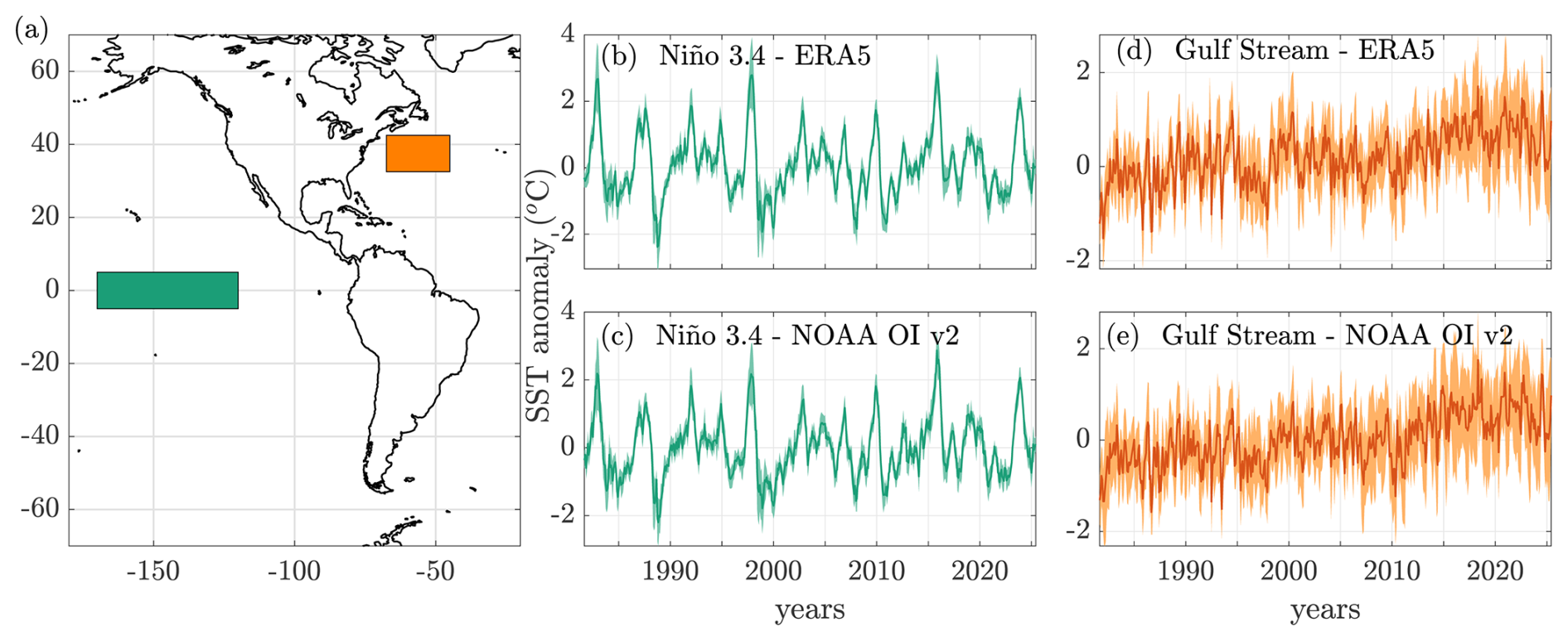
Figure 1 Panel (a) highlights the regions of interest: Niño 3.4 (in green), and the Gulf Stream (in orange). Panels (b) and (c) show the SST anomaly in the Niño 3.4 region, and panels (d) and (e), in the Gulf Stream region, calculated from ERA5 (b, d) and NOAA OI v2 (c, e) datasets. In panels (b)–(e), the thick lines represent the spatial mean of the anomalies, while the shading indicates the spatial standard deviation.

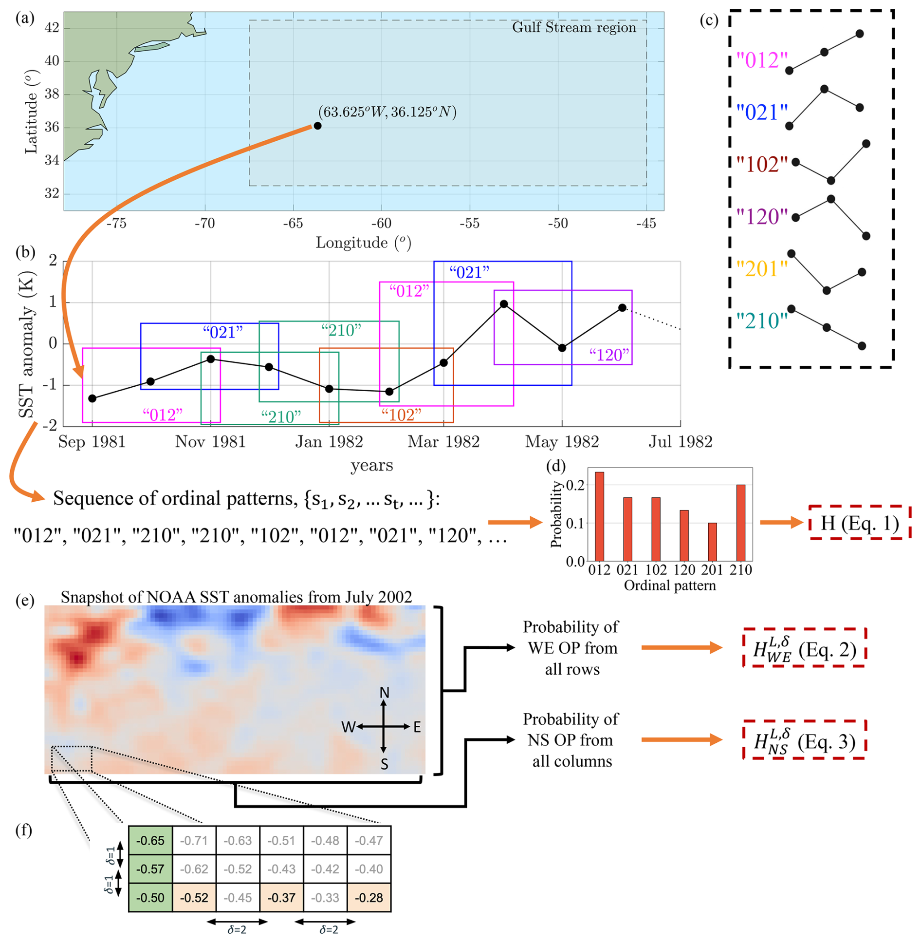
Figure 2 Illustration of the procedure used to define ordinal patterns (OPs) and to calculate the permutation entropy (PE) of patterns of length L. (a) Location of a grid point inside the Gulf Stream region. (b) The temporal evolution of NOAA SST anomaly at this grid point (sequence x) is represented by a sequence of “temporal” OPs (sequence s) that are defined by the relative ordering of L=3 consecutive (δ=1) data values. (c) The six possible orderings represent the six possible OPs. (d) The OPs' probabilities are estimated by counting the number of times each OP occurs in the sequence s, and the permutation entropy (PE), H(L,δ), is calculated using Eq. (1). (e) Snapshot of NOAA SST anomalies in the Gulf Stream region in July 2002. A row of this snapshot defines a sequence of consecutive data values, x, along the WE direction, from which spatial OPs are defined using the same rule as in (b). From the probabilities of the OPs defined over all the rows in the snapshot, the value of the entropy, for July 2002, $H_{\text{WE}}^{L,\mathit{\delta }}$, is calculated using Eq. (2). Repeating this procedure for the columns (along the NS direction) gives $H_{\text{NS}}^{L,\mathit{\delta }}$ (Eq. 3). (f) Detail of how the spatial lag, δ, is used to define spatial OPs: The three consecutive values (δ=1) marked in green in the NS direction, $[\mathrm{1.1},-\mathrm{1.4},\mathrm{4.1}]$, are represented by pattern “102”, while the three values marked in orange, lagged δ=2 in the WE direction, $[\mathrm{3.2},\mathrm{4.4},\mathrm{1.3}]$, are represented by pattern “120”.

The ordinal symbolic transformation requires defining only two parameters: the symbol length, L, and the lag, δ. These parameters are used to associate, to a vector v_i whose components are L data points lagged by δ, a symbol s_i that is known as ordinal pattern (OP),

$$\begin{array}{ll}{\displaystyle }& {\displaystyle }{v}_i(L,\mathit{\delta })=[x_i,x_{i+\mathit{\delta }},x_{i+\mathrm{2}\mathit{\delta }},\mathrm{\dots },x_{i+(L-\mathrm{1})\mathit{\delta }}]\\ {\displaystyle }& {\displaystyle }\to s_i(L,\mathit{\delta })=\left[\mathit{\pi }\right(i),\mathit{\pi }(i+\mathit{\delta }),\mathrm{\dots },\mathit{\pi }(i+(L-\mathrm{1})\mathit{\delta }\left)\right].\end{array}$$

Here π(⋅) is the permutation index that sorts the components of v_i in ascending order: $x_{\mathit{\pi }\left(i\right)}\le x_{\mathit{\pi }(i+\mathit{\delta })}\le \mathrm{\dots }\le x_{\mathit{\pi }(i+(L-\mathrm{1}\left)\mathit{\delta }\right)}$. The number of possible permutations, that is, of possible patterns, grows as L!. The six possible patterns of length L=3 are shown in Fig. 2c and examples are shown in Fig. 2f: the vector $[\mathrm{1.1},-\mathrm{1.4},\mathrm{4.1}]$ is represented by pattern “102” while $[\mathrm{3.2},\mathrm{4.4},\mathrm{1.3}]$ is represented by “120”, etc. We remark that the ordinal transformation takes into account relative values, not absolute ones.

Applying this transformation to every v_i(L,δ) with $i=\mathrm{1},\mathrm{\dots },n=N-(L-\mathrm{1})\mathit{\delta }$, gives a sequence of n ordinal patterns, $s(L,\mathit{\delta })=\mathit{\{}{s}_{\mathrm{1}},s_{\mathrm{2}},\mathrm{\dots },s_i,\mathrm{\dots },\mathrm{\dots }{s}_n\mathit{\}}$. Labeling the possible patterns (symbols) from k=1 to k=L! (for L=3, k=1 corresponds to pattern “012”, k=2 to pattern “021”, etc., as illustrated in Fig. 2c), we can count the number of times each pattern appears in s. Let n^k be the number of times the kth pattern appears. Then, the probability of this pattern is $p^k(L,\mathit{\delta })=n^k/n$. Figure 2d displays an example of six probabilities of patterns of length L=3. The permutation entropy (PE) is then defined as Shannon's entropy of the probabilities (Bandt and Pompe, 2002):

$$\begin{array}{}\text{(1)}& {\displaystyle }{\displaystyle }H(L,\mathit{\delta })=-{\displaystyle \frac{\mathrm{1}}{\log \left(L\mathrm{!}\right)}}\sum _{k=\mathrm{1}}^{L\mathrm{!}}{p}^k(L,\mathit{\delta })\log \left(p^k(L,\mathit{\delta })\right).\end{array}$$

The coefficient $\mathrm{1}/\log \left(L\mathrm{!}\right)$ normalizes H(L,δ) between 0–1 and enables the comparison between values obtained from ordinal pattens of different lengths. A small entropy value is obtained where one pattern predominates (this occurs when the sequence $x=\mathit{\{}{x}_{\mathrm{1}},x_{\mathrm{2}},\mathrm{\dots },x_i,\mathrm{\dots },x_N\mathit{\}}$ is periodic, or when it has a strong trend), whereas a high entropy value is obtained when all symbols are almost equally probable, which normally occurs when the sequence x is fully stochastic.

To estimate the patterns' probabilities with good statistics, the number of symbols, $n=N-(L-\mathrm{1})\mathit{\delta }$, needs to be much larger than the number of possible patterns, L!. In practical terms, this limits the values of L to the range from 3 to 6. Here, unless explicitly stated, we use L=4 and use different values of δ to tune the spatial scale of the analysis.

3.2 Symbol orientations in 2D spatio-temporal gridded data

The SST anomalies in the two regions of interest are represented as the time evolution of 2-dimensional N×M gridded datasets, X_i,j(t) with $i\in \mathit{\{}\mathrm{1},\mathrm{\dots },N\mathit{\}},j\in \mathit{\{}\mathrm{1},\mathrm{\dots },M\mathit{\}},t\in \mathit{\{}\mathrm{1},\mathrm{\dots },T\mathit{\}}$, where the index i corresponds to different latitudes, the index j to different longitudes, and T is the number of time steps in the series. Given L and δ, at each time step, t, we apply the ordinal transformation using two spatial orientations: in the North–South (NS) direction, the ordered series x is defined from the values, at time t, of the columns of the grid, and in the West–East (WE) direction, from the rows of the grid, see Fig. 2e and f. In each column we can define $N-(L-\mathrm{1})\mathit{\delta }$ OPs, while in each row, we can define $M-(L-\mathrm{1})\mathit{\delta }$ OPs. Defining OPs over all the columns the total number of OPs defined along the NS direction is $M\left(N-(L-\mathrm{1})\mathit{\delta }\right)$, and defining OPs over all the rows, the total number of OPs defined along the WE direction is $N\left(M-(L-\mathrm{1})\mathit{\delta }\right)$. An important advantage of this methodology for the analysis of climatological data is its flexibility, because the OP orientation is not limited to NS and WE directions, but other orientations can be selected for the analysis.

We also remark that L and δ allow tuning the spatial scale of the analysis. In the original application of permutation entropy to time series analysis (Bandt and Pompe, 2002), we can interpret L and δ as parameters that allow a nonlinear embedding of a time series in a L! dimensional space, because at each time, an ordinal pattern can be defined, and the number of possible patterns is L!. In the spatial approach, the parameters L and δ have a similar role: they allow to embed a set of L gridded data points in a L! dimensional space.

From the probabilities of the OPs defined at time t along the NS and WE directions, $p_{\text{WE}}^k\left(t\right)$ and $p_{\text{NS}}^k\left(t\right)$ respectively, we compute two spatial permutation entropies at time t:

$$\begin{array}{}\text{(2)}& {\displaystyle }& {\displaystyle }{H}_{\text{WE}}^{L,\mathit{\delta }}\left(t\right)=-{\displaystyle \frac{\mathrm{1}}{\log \left(L\mathrm{!}\right)}}\sum _{k=\mathrm{1}}^{L\mathrm{!}}{p}_{\text{WE}}^k\left(t\right)\log \left(p_{\text{WE}}^k\left(t\right)\right),\text{(3)}& {\displaystyle }& {\displaystyle }{H}_{\text{NS}}^{L,\mathit{\delta }}\left(t\right)=-{\displaystyle \frac{\mathrm{1}}{\log \left(L\mathrm{!}\right)}}\sum _{k=\mathrm{1}}^{L\mathrm{!}}{p}_{\text{NS}}^k\left(t\right)\log \left(p_{\text{NS}}^k\left(t\right)\right).\end{array}$$

Since SST anomalies vary over time, the ordinal probabilities vary over time and thus, the entropies vary over time. $H_{\text{NS}}^{L,\mathit{\delta }}\left(t\right)$ and $H_{\text{WE}}^{L,\mathit{\delta }}\left(t\right)$ will be close to 1 when there is no spatial order in the data (all OPs are equally probable), and will be <1 when there are spatial structures, such as gradients in the NS or in the WE direction, that make some OPs more or less probable.

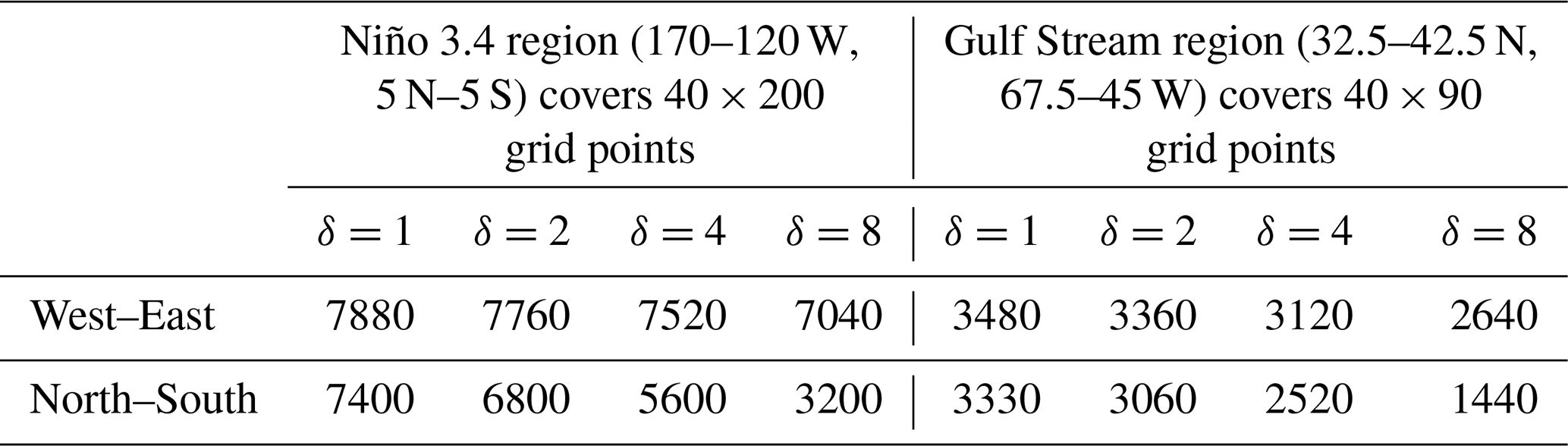
In this work, we consider symbols defined by L=4 grid points and a spatial lag up to δ=8, as these are the largest values that allow us, given the size of the two regions studied, to estimate with good statistics the probabilities of the L!=24 possible patterns. Table 1 shows the number of symbols (defined by L=4 grid points in the geographical region analyzed) when a spatial lag of δ=1, 2, 4, and 8 is used. We see that the lowest number (in the Gulf stream with δ=8) is ≫24. We tested the robustness of our results with respect to L, and found similar results with L=3 and L=5 (see Figs. B3–B7 of Appendix B).

Table 1 Number of symbols (ordinal patterns), for L=4, defined in the two regions analyzed, for each orientation, and for each spatial lag (δ) considered.

3.3 Entropy calculated from the distribution of data values

In this work we also compare the permutation entropy with the conventional way of calculating Shannon entropy of a spatio-temporal field, X_i,j(t), from the distribution of its data values,

$$\begin{array}{}\text{(4)}& {\displaystyle }{\displaystyle }{H}_{\text{hist}}\left(t\right)=-{\displaystyle \frac{\mathrm{1}}{\log m}}\sum _{k=\mathrm{1}}^m{p}^k\left(t\right)\log \left(p^k\left(t\right)\right).\end{array}$$

Here p^k(t) is the probability that X_i,j(t) is in the k state and m is the number of possible states. p^k(t) is estimated from histograms of m bins of equal size, that represent the possible states. H_hist(t)=1 when p^k(t)=1 and $p^j\left(t\right)=\mathrm{0}\forall j\ne k$ (only one bin is occupied), and H_hist(t)=0 if $p^k\left(t\right)=\mathrm{1}/m\forall k$ (the distribution of values is uniform). To compare with SPE values calculated with ordinal patterns of length L, we select the number of bins equal to the number of possible ordinal patterns, m=L!. To calculate H_hist(t) all the data points of X_i,j(t) in the regions of interest are used. As explained in Sect. 2, ERA5 and NOAA have 40×200 grid points in the Niño region and 40×90 in the Gulf Stream region.

3.4 Distance and cross-correlations measures used to compare SST-ERA5 and SST-NOAA

In this work we demonstrate that spatial permutation entropy can detect differences in ERA5 and NOAA SST products, and an important question is whether such differences can also be detected using standard correlation or distance measures. Therefore, we also compare SST anomaly values using the Average Absolute Difference (AAD), the Pearson's spatial cross-correlation coefficient (r), and the Spatial Mutual Information (SMI), which is a non-linear cross-correlation measure (Celik, 2016; Kumar and Bhandari, 2022).

The Average Absolute Difference is defined as:

$$\begin{array}{}\text{(5)}& {\displaystyle }{\displaystyle }\text{AAD}\left(t\right)={〈\left|X_{i,j}\left(t\right)-Y_{i,j}\left(t\right)\right|〉}_{i,j},\end{array}$$

where X_i,j(t) and Y_i,j(t) represent the two gridded datasets, ERA5 and NOAA, and ${〈\cdot 〉}_{i,j}$ represents the spatial average in the analyzed region, at time t.

Pearson's spatial cross-correlation coefficient is defined as:

$$\begin{array}{}\text{(6)}& {\displaystyle }{\displaystyle }r\left(t\right)={\displaystyle \frac{{\mathit{\sigma }}_{X,Y}\left(t\right)}{{\mathit{\sigma }}_X\left(t\right){\mathit{\sigma }}_Y\left(t\right)}},\end{array}$$

where σ_X(t), σ_Y(t) and σ_X,Y(t) are the spatial standard deviations and the spatial covariance of X_i,j(t) and Y_i,j(t) at time t. To calculate ADD and r, all the data points of X_i,j(t) and Y_i,j(t) in the regions of interest are used. As explained in Sect. 2, ERA5 and NOAA both have 40×200 grid points in the Niño region and 40×90 in the Gulf Stream region.

The spatial mutual information (SMI) of X_i,j(t) and Y_i,j(t) at time t is defined as:

$$\begin{array}{}\text{(7)}& {\displaystyle }{\displaystyle }\text{SMI}\left(t\right)=H_X\left(t\right)+H_Y\left(t\right)-H_{X,Y}\left(t\right),\end{array}$$

where $H_X\left(t\right)=-{\sum }_{k=\mathrm{1}}^{m_X}{p}_X^k\log \left(p_X^k\right)$ and $H_Y\left(t\right)=-{\sum }_{l=\mathrm{1}}^{m_Y}{p}_Y^l\log \left(p_Y^l\right)$ are the Shannon entropies of X_i,j(t) and Y_i,j(t), and H_X,Y(t) denote their joint entropy,

$$\begin{array}{}\text{(8)}& {\displaystyle }{\displaystyle }{H}_{X,Y}\left(t\right)=-\sum _{k=\mathrm{1}}^{m_X}\sum _{l=\mathrm{1}}^{m_Y}{p}^{k,l}\left(t\right)\log \left(p^{k,l}\left(t\right)\right),\end{array}$$

where m_X and m_Y are the numbers of possible states of X and Y respectively, and p^k,l(t) denotes the joint probability that X_i,j(t) is in state k and Y_i,j(t) in state l.

We calculate SMI using two approaches: the conventional one, in which the distributions of values of X_i,j(t) and Y_i,j(t) are divided in an equal number of bins, $m_X=m_Y=m$, of equal size, that represent the possible states, and the ordinal approach, in which the possible states are the possible ordinal patterns, defined over Lδ-lagged gridded points, aligned along the NS or WE directions. Then, in the ordinal approach, $m_X=m_Y=L\mathrm{!}$. We refer to the mutual information calculated in these ways as SMI_hist(t), ${\text{SMI}}_{\text{NS}}^{L,\mathit{\delta }}\left(t\right)$ and ${\text{SMI}}_{\text{WE}}^{L,\mathit{\delta }}\left(t\right)$.

Since for L=4 OPs there are $m=L\mathrm{!}=\mathrm{24}$ possible patterns, which are the possible “states”, to calculate SMI_hist the probabilities $p_X^k\left(t\right)$ and $p_Y^l\left(t\right)$ were estimated from histograms with m=24 bins of equal size, and the joint probability, p^k,l(t), was estimated from 2D histograms with 24×24 bins of equal size. In this way, the SMI values were obtained from probabilities defined over the same number of possible states. To calculate all the histograms, all the data points of in the regions of interest were used. To test the robustness of the results, we also calculated ${\text{SMI}}_{\text{NS}}^{L,\mathit{\delta }}\left(t\right)$ and ${\text{SMI}}_{\text{WE}}^{L,\mathit{\delta }}\left(t\right)$ using ordinal patterns of length L=3 and compared with SMI_hist(t) using histograms with 6 bins and joint histograms with 6×6 bins, and obtained very similar results (shown in Fig. B7 of Appendix B).

4 Results

4.1 Detecting transitions with spatial permutation entropy analysis

Figure 3 displays the temporal evolution of the spatial permutation entropy, calculated from the probabilities of L=4 OPs defined from the values of SST anomalies in neighboring grid point (i.e. the spatial lag is δ=1). Panels (a) and (d) display $H_{\text{NS}}^{L=\mathrm{4},\mathit{\delta }=\mathrm{1}}$ for the two datasets analyzed, ERA5 in blue and NOAA OI v2 in red, in the two regions analyzed: panel (a) corresponds to the Niño 3.4 region, and panel (c), to the Gulf Stream region. Results are presented from the beginning of the datasets (1940 for ERA5 and 1981 for NOAA OI v2). Panels (b) and (e), instead, display $H_{\text{WE}}^{L=\mathrm{4},\mathit{\delta }=\mathrm{1}}$, also in the two regions and for the two datasets under analysis. For comparison, panels (c) and (f) show the entropy calculated from the distribution of data values, H_hist. As explained in Sect. 3.3, to estimate the distribution we use histograms with 24 equal bins.

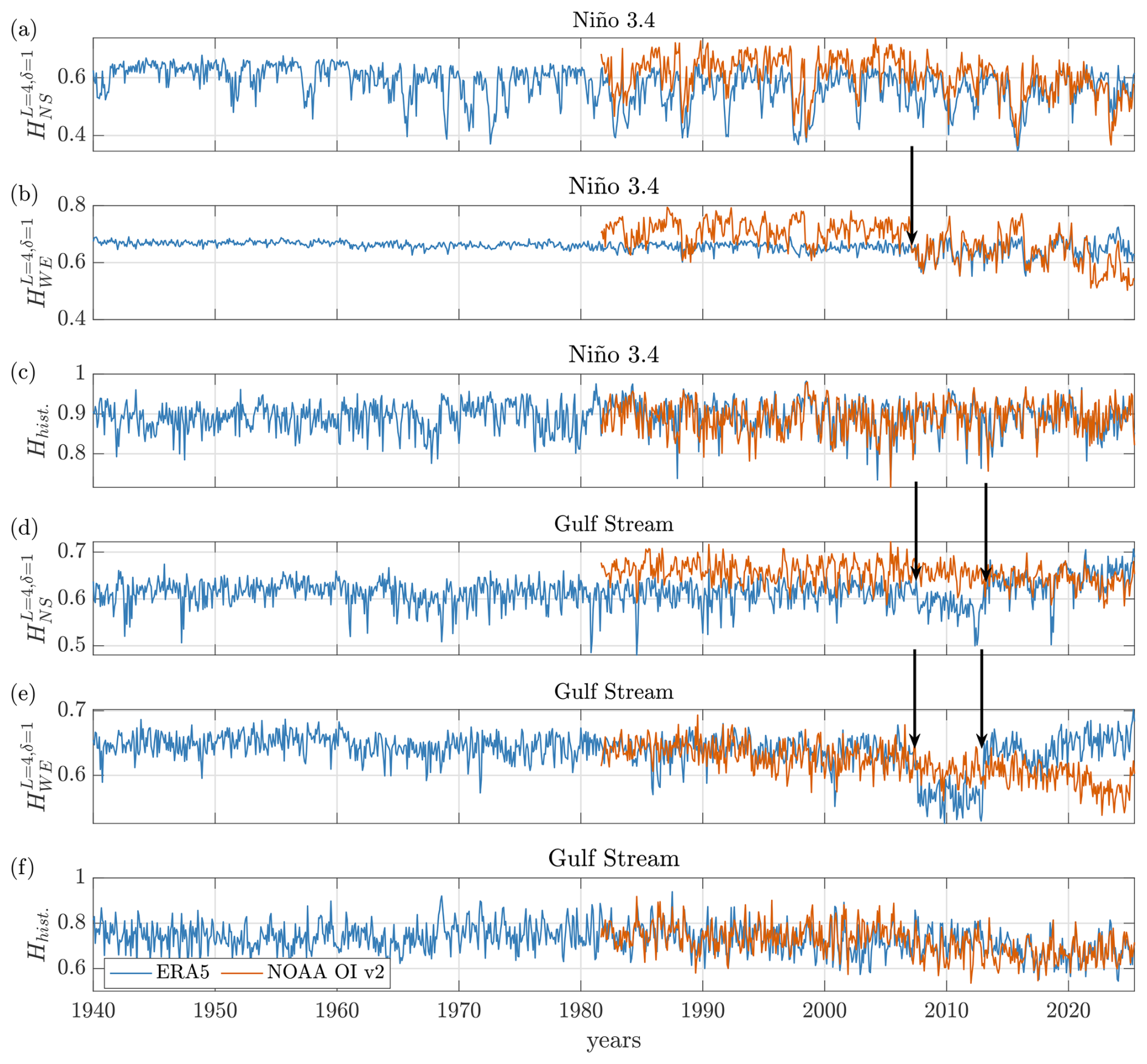
Figure 3 Entropies of (a–c) Niño 3.4 region; (d–f) Gulf Stream region. Panels (a), (b), (d), and (e) show the spatial permutation entropy calculated with spatial lag δ=1, while panels (c) and (f) show the usual entropy obtained from the distributions of the SST anomaly values. Blue lines correspond to the entropy from the ERA5 dataset, red lines to the entropy from the NOAA OI v2 dataset, and the black arrows indicate the change points detected by the PELT algorithm in the ERA5 dataset.

In the Niño 3.4 region, panel (a) shows that the evolution of $H_{\text{NS}}^{L=\mathrm{4},\mathit{\delta }=\mathrm{1}}$ for ERA5 and NOAA OI v2 is quite similar. However, panel (b) shows differences in the evolution of $H_{\text{WE}}^{L=\mathrm{4},\mathit{\delta }=\mathrm{1}}$ which persist until 2007. After 2007 the differences reduce until 2022, when the two values of $H_{\text{WE}}^{L=\mathrm{4},\mathit{\delta }=\mathrm{1}}$ diverge again. The years when these transitions occur coincide with the switch of the sea-surface boundary condition of ERA5, from HadISST2 to OSTIA, in 2007 (Hersbach et al., 2020), and with the inclusion of MeteOp-C satellite data in NOAA's dataset in November 2021 (Jonasson et al., 2020).

Although many transitions can be identified by visual inspection, to objectively identify change points in the temporal evolution of the entropies (and in all the quantifiers used), we employed a well-known unsupervised change point detection (CPD) algorithm, the Pruned Exact Linear Time (PELT) (Killick et al., 2012). We tested the significance of the detected change points by PELT using a surrogate analysis, and their robustness against variations of the penalty parameter (see Appendix A for details).

The arrows in Fig. 3 indicate the change points detected by the PELT algorithm. We note that no change point is detected in panel (a), but a change point is detected in panel (b), in 2007. In the Gulf Stream region, panel (d) shows differences between the values of $H_{\text{NS}}^{L=\mathrm{4},\mathit{\delta }=\mathrm{1}}$ of ERA5 and NOAA OI v2, which become relatively small after 2013, a fact that could be due to the update of the background error covariances in OSTIA in January 2013 (Good et al., 2020; Roberts-Jones et al., 2016). Panel (e) also shows considerable differences between the values of H_WE, from 2021 onward, and which could be due to the inclusion of MetOp-C AVHRR data in NOAA OI v2 (Huang et al., 2023). While change points in 2007 and 2013 are returned by the PELT algorithm, the one in 2021, although significant in the NOAA signal, does not pass the robustness test (See Table. A1 in Appendix A). For the same level of statistical significance with respect to surrogates and robustness with respect to variations of the penalty parameter, no change points are detected for H_hist (panels c and f).

Summarizing, most changes that can be identified by visual inspection are consistent with changes returned by the PELT algorithm when used to analyze $H_{\text{NS}}^{L=\mathrm{4},\mathit{\delta }=\mathrm{1}}$(ERA5), $H_{\text{NS}}^{L=\mathrm{4},\mathit{\delta }=\mathrm{1}}$(NOAA OI v2), $H_{\text{WE}}^{L=\mathrm{4},\mathit{\delta }=\mathrm{1}}$(ERA5) and $H_{\text{WE}}^{L=\mathrm{4},\mathit{\delta }=\mathrm{1}}$(NOAA OI v2) in Niño 3.4 and Gulf Stream regions. The PELT change points are:

1. A first transition occurs in ERA5 in 2007, which we interpreted as due to the change of the sea-surface boundary conditions: the inclusion of OSTIA in 2007. This transition is associated to change points that are identified in $H_{\text{NS}}^{L=\mathrm{4},\mathit{\delta }=\mathrm{1}}$ and $H_{\text{WE}}^{L=\mathrm{4},\mathit{\delta }=\mathrm{1}}$ in the Gulf Stream region, and in $H_{\text{WE}}^{L=\mathrm{4},\mathit{\delta }=\mathrm{1}}$ in the Niño 3.4 region, but not in $H_{\text{NS}}^{L=\mathrm{4},\mathit{\delta }=\mathrm{1}}$ in the Niño 3.4 region. We remark that ENSO is a large-scale phenomenon characterized by large zonal temperature changes, and in the Niño 3.4 region, the spatial permutation entropy best captures differences along the direction of the largest gradients.

2. A second transition occurs in ERA5 in 2013, which we interpreted as due to the update of OSTIA. This transition is associated to change points that are identified in the Gulf stream region, both in $H_{\text{NS}}^{L=\mathrm{4},\mathit{\delta }=\mathrm{1}}$ and $H_{\text{WE}}^{L=\mathrm{4},\mathit{\delta }=\mathrm{1}}$, but not in the Niño 3.4 region.

Figure 4 displays the entropies as in Fig. 3, but now the ordinal patterns are defined with non-neighboring grid points. Specifically, the grid points are spaced by a lag δ=8 that corresponds to 2°. Now we see that the temporal evolution of the entropies of ERA5 and NOAA OI v2 is consistent, in the two regions and for the two orientations. Discrepancies are small: not only the fluctuations are highly correlated, but also, the trends are similar, but no change points are detected at this scale. For the Nino 3.4 region, although $H_{\text{NS}}^{L=\mathrm{4},\mathit{\delta }=\mathrm{8}}$ (panel a) does not present a significant trend, in panel (b) we see that $H_{\text{WE}}^{L=\mathrm{4},\mathit{\delta }=\mathrm{8}}$ from the two datasets display a negative trend. This trend is interpreted as due to the inhomogeneous long-term SST variations over the equatorial Pacific, since over the years, SST has warmed in the west and cooled in the east (Xie et al., 2010; Wills et al., 2022). This represents an intensifying westward large-scale gradient over the Niño 3.4 region that can make the patterns that encode monotonic increasing or decreasing, such as “0123” and “3210”, more prevalent than those that encode an oscillation (See Fig. B15 of Appendix B), thus decreasing the entropy. However, low SPE values do not always imply that the “0123” and “3210” patterns dominate, and a careful inspection of the patterns' probabilities is needed in order to be able to confidently draw conclusions.

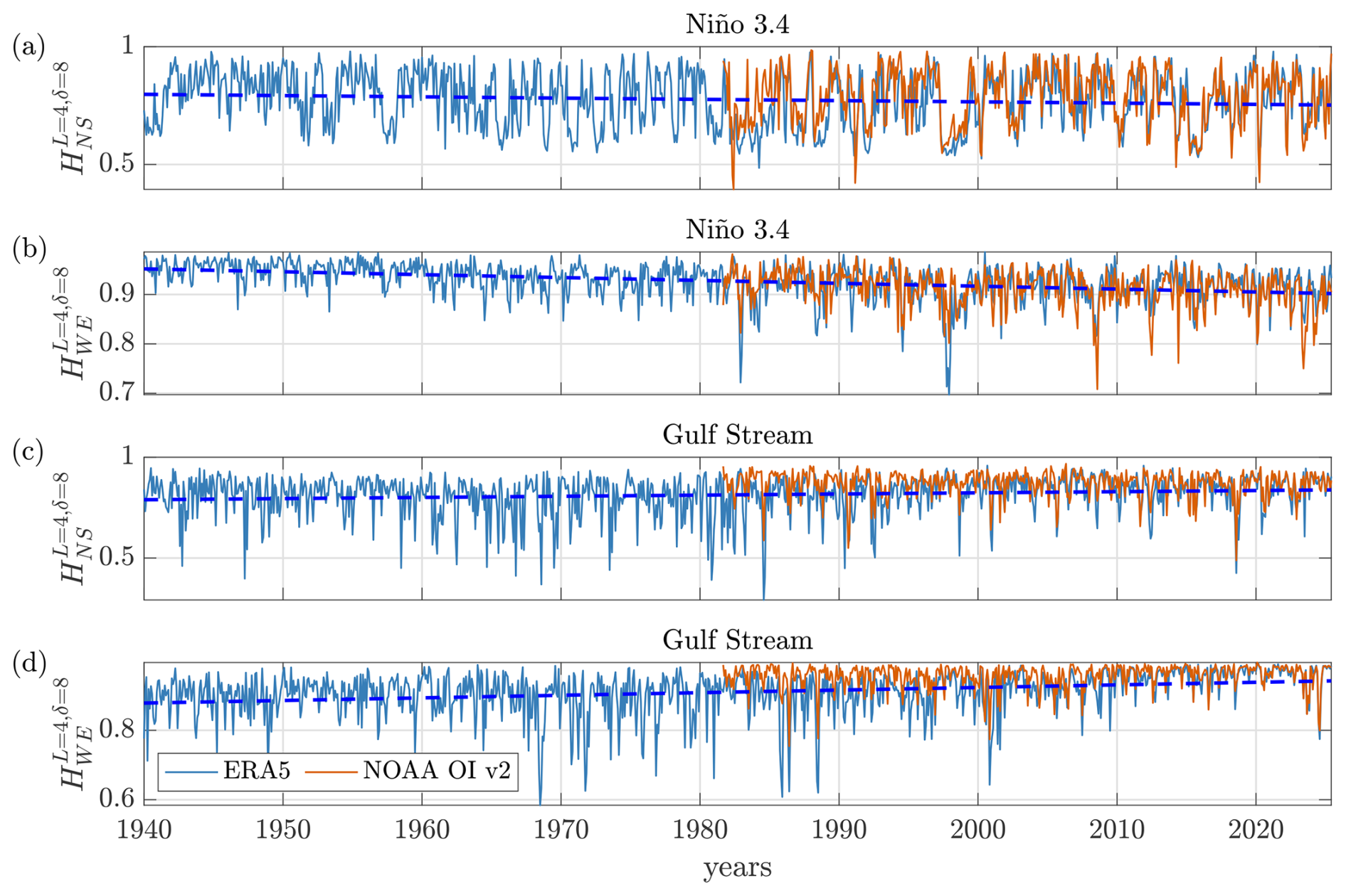
Figure 4 Entropies calculated with δ=8 in (a, b) Niño 3.4 region; (c, d) Gulf Stream region. A better agreement between NOAA OI v2 and ERA5 signals is observed with δ=8 than with δ=1 (Fig. 3). Dashed blue lines indicate linear fits of ERA5 entropy signals; which linear coefficients are: (a) $-\mathrm{5.04}{\mathrm{e}}^{-\mathrm{4}}{\text{yr}}^{-\mathrm{1}}$ (p value=0.18), (b) $-\mathrm{5.52}{\mathrm{e}}^{-\mathrm{4}}{\text{yr}}^{-\mathrm{1}}$ ($p\text{ value}=\mathrm{2.0}{\mathrm{e}}^{-\mathrm{10}}$), (c) $\mathrm{7.20}{\mathrm{e}}^{-\mathrm{4}}{\text{yr}}^{-\mathrm{1}}$ (p value=0.0016), (d) $\mathrm{7.56}{\mathrm{e}}^{-\mathrm{4}}{\text{yr}}^{-\mathrm{1}}$ ($p\text{ value}=\mathrm{2.3}{\mathrm{e}}^{-\mathrm{8}}$). The negative trend in (b) can be due to the strengthening westward of large-scale gradient in the Niño 3.4 region, while the positive trends in (c) and (d) reveal the decrease of spatial structures.

In the Gulf Stream region, which is also heating due to global warming (Seidov et al., 2017; Todd and Ren, 2023), H_WE and H_NS in ERA5 and in NOAA present a positive trend, which reveals a decrease of spatial structure, as it means that the different symbols become equally probable. In this case, since the northwest part is warming faster than the rest of this area (Bulgin et al., 2020), it decreases the climatological gradient of the SST across the Gulf stream, thus homogenizing the entire region, and the resulting symbols resemble more closely those of random fluctuations (See Fig. B15 of Appendix B).

To check the robustness of our results, we also performed the analysis after removing the linear temporal trend in each grid point, and obtained similar results, shown in Figs. B9–B12 of Appendix B. In these figures we also include the analysis of the raw SST data – including the seasonal cycle.

Figure 5 shows the same entropy signals as Figs. 3 and 4 for the Niño 3.4 region, but in the period 1981–2025, and also shows the mean SST anomaly of this region (black line, right vertical axis) computed from the NOAA dataset.Table 2 displays the Pearson cross-correlation coefficients between the entropies computed from NOAA and ERA5, and the corresponding SST anomaly. In this Table we observe a good agreement between NOAA and ERA5 in Niño 3.4, in terms of the sign and magnitude of the cross-correlation coefficient, for all the entropies. In panel (b) of Fig. 5, we can see that $H_{\text{WE}}^{L=\mathrm{4},\mathit{\delta }=\mathrm{1}}$ from the NOAA dataset is positively correlated with the SST anomaly (the Pearson cross-correlation coefficient is r=0.42), most clearly between 2007–2022 (r=0.70). The $H_{\text{WE}}^{L=\mathrm{4},\mathit{\delta }=\mathrm{1}}$ values are the largest during El Niño years, capturing the decrease in SST gradients along the longitudinal direction. For ERA5, this correlation is strongest from 2007 onward (r=0.57). In contrast, $H_{\text{NS}}^{L=\mathrm{4},\mathit{\delta }=\mathrm{1}}$ (panel a) is negatively correlated with the SST anomaly ($r=-\mathrm{0.23}$ for NOAA, and $r=-\mathrm{0.20}$ for ERA5), thus during some El Niño events (such as 1997–1998 and 2015–2016 years) the entropy decreases, reflecting the north-south gradients, one in the Northern Hemisphere and one in the Southern Hemisphere, that occur as the equatorial zone is warmer than the north-south edges of the region. This is also observed for some La Niña events, such as the one in 1988–1989 or in 1998–1999.

Table 2 Pearson correlation coefficients obtained between the mean SST anomaly and the entropy signals, for L=4 and different lags, and for both ocean regions.

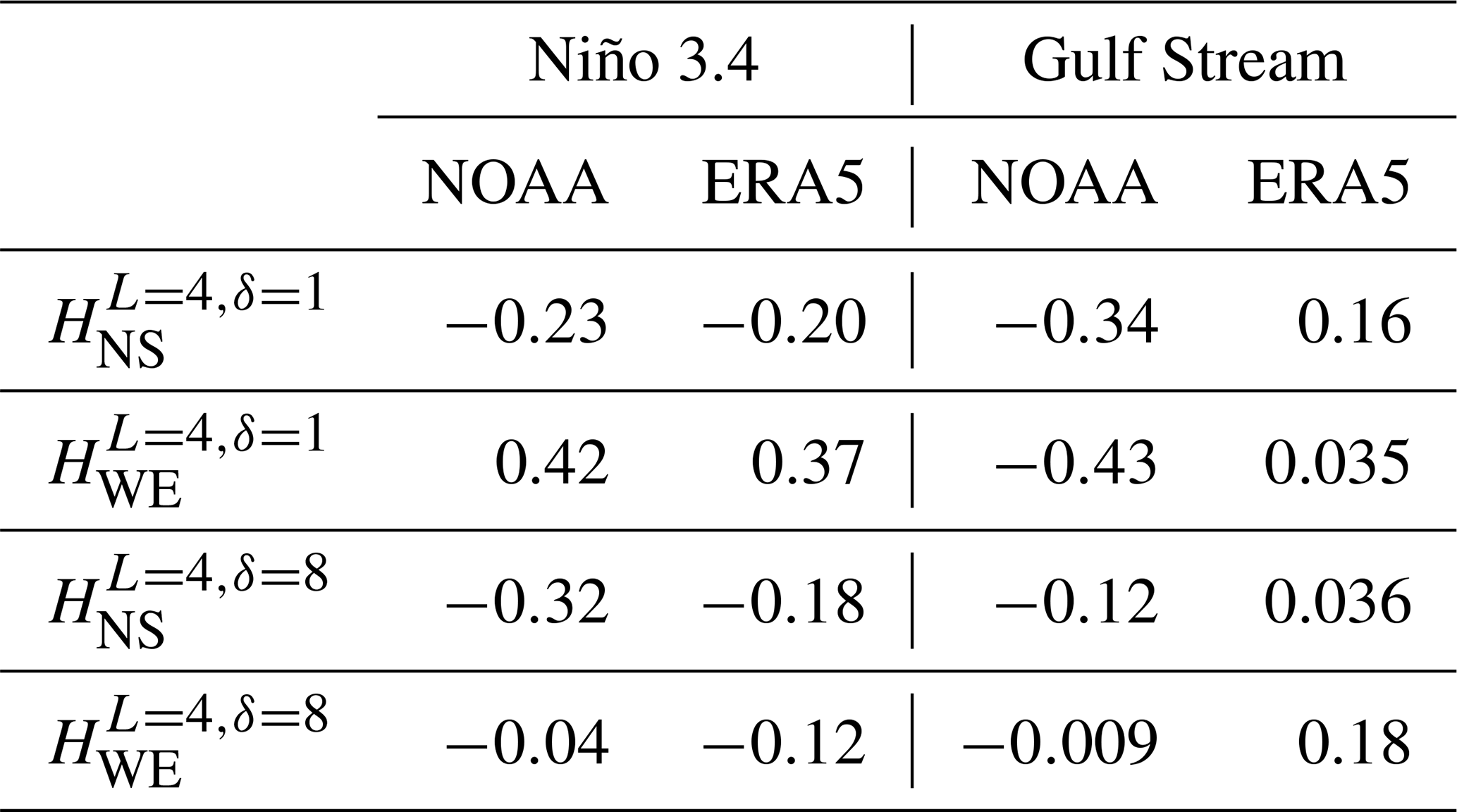
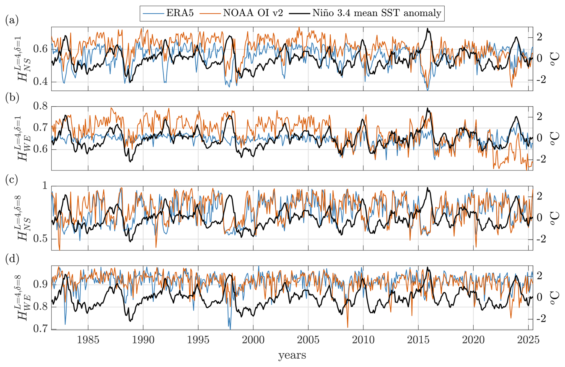
Figure 5 Analysis of the Niño 3.4 region, in the time interval in which ERA5 and NOAA OI v2 datasets are available (1981–2025). Panels (a)–(d) display the temporal evolution of the SST anomaly (black line, right vertical axis) computed from the NOAA dataset (a similar curve would be obtained from ERA5, as shown in Fig .1), and the temporal evolution of the spatial permutation entropy (red and blue, left vertical axis) calculated with ordinal patterns with NS (a, c) and WE (b, d) orientation. In (a), (b) the spatial lag used to define the ordinal patterns is δ=1, in (c), (d) δ=8. The Pearson correlation coefficients between the mean SST anomaly and the entropy signals are shown in Table 2. In panel (a), where the OPs are aligned along the NS direction, the entropy signals are negatively correlated with the SST anomaly, while in panel (b), where the OPs aligned along the WE direction, the entropy signals and the SST anomaly are positively correlated.

For the same analysis, but with δ=8, sudden drops of $H_{\text{WE}}^{L=\mathrm{4},\mathit{\delta }=\mathrm{8}}$ (Fig. 5d) can be observed, and some correlate with El Niño events, such as the ones in 1982–1983 or 1997–1998, but also at the end of a strong La Niña in 2008. In these cases (see Fig. B1), a WE gradient is formed due to the strong warming of the eastern Pacific, which dominates at this long spatial scale, and in consequence, pattern “0123” prevails (thus, the entropy drops). In contrast, for δ=1, the distribution of ordinal probabilities presents larger contributions of two patterns, “0123” and “3210”, so the entropy is higher. Some drops are also seen in the temporal evolution of $H_{\text{NS}}^{L=\mathrm{4},\mathit{\delta }=\mathrm{8}}$ (Fig. 5c), although at this scale $H_{\text{NS}}^{L=\mathrm{4},\mathit{\delta }=\mathrm{8}}$ cannot capture the NS gradients appropriately. In fact, for δ=8 the ordinal patterns span 6° (more than half of the region length in this direction), because the data points are separated by $\mathrm{0.25}\mathit{°}\times \mathrm{8}=\mathrm{2}\mathit{°}$ and thus, L=4 data points that define a pattern cover a distance of $\mathrm{3}\times \mathrm{2}\mathit{°}=\mathrm{6}\mathit{°}$). As El Niño develops in a waveguide between 5° S–5° N, the SST anomalies evolve particularly in that area, and the NS gradients are highly concentrated near the equator. Therefore, they can be seen with δ=1, but if δ=8 is used, the OPs can include the SST variations north and south of the equator (SST decreases north and south of the equator), mixing both gradients. This does not occur in the longitudinal WE direction, as the WE gradients have a larger spatial scale. To gain further insight, we inspected the temporal evolution of the ordinal probabilities, and found that their variation is consistent with the interpretation of the gradients that are captured when using using different δs. Videos showing how the probabilities of NS and WE OPs change over time can be found in the Video Supplement.

We also performed this analysis in the Gulf Stream region. The results, displayed in Fig. B8 and Table 2 reveal that there is no consistent correlation between the entropy signals and the SST anomalies in the two datasets (i.e. the cross-correlation coefficients obtained from NOAA and ERA5 differ both in magnitude and sign). We speculate that this is due to the fact that SST anomalies, even when aggregated at the basin scale, do not present a smooth behavior (as in the Niño 3.4 region).

4.2 Comparison between ERA5 and NOAA datasets

To analyze similarities and differences between ERA5 and NOAA, in this section we only consider the period when both datasets are available (1981–2024). To visualize the effect of the spatial lag between the grid points, Fig. 6 displays the entropies (as done in Figs. 3 and 4), for grid points that are consecutive (i.e. they are separated by 0.25°, that is, δ=1), that are separated by 0.5° (δ=2), by 1° (δ=4), and by 2° (δ=8). Therefore, in this figure, the left and right columns display the same entropies as in Figs. 3 and 4.

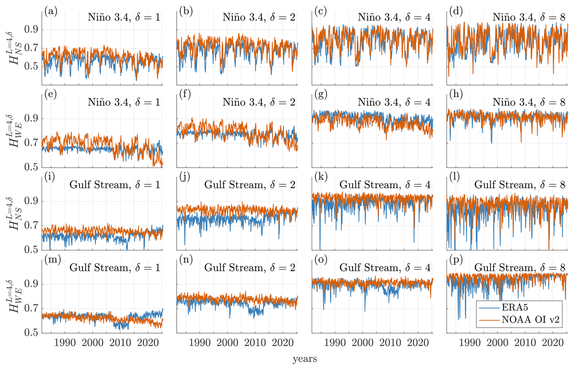
Figure 6 Effect of the lag between grid points. Panels (a)–(h) correspond to the Niño 3.4 region, and (i)–(p) to the Gulf Stream region. We can see that as δ increases, the entropy differences gradually decrease, revealing that the SPE analysis captures the differences between ERA5 and NOAA datasets at small spatial scales.

We observe that as δ increases the behavior of $H_{\text{NS}}^{L,\mathit{\delta }}$ and $H_{{\mathrm{WE}}^{L,\mathit{\delta }}}$ for the two datasets converge, which indicates that the differences found between ERA5 and NOAA occur mainly at short spatial scales, while at long scales, linear trends in the temporal evolution of the entropies are consistently identified in both, ERA5 and NOAA. We also notice that, as δ increases, so do the entropies, suggesting that the gradients become less pronounced as the spatial scale increases.

To perform a quantitative comparison between the datasets, we begin by analyzing their SMI, reported in Fig. 7. In panels (a)–(h) we report SMI^L,δ estimated from ordinal probabilities, in particular δ=1 for panels (a)–(d) and δ=8 for panels (e)–(h), while panels (i) and (j) display SMI_hist. estimated from the probabilities of values of SST anomalies.

When SMI is calculated from the ordinal probabilities, in the two regions and for the two orientations, we can see that it increases with time, which reveals that the amount of information shared by the datasets. In particular, the probability that the same symbols occur in the same locations and at the same time in both datasets increases with time (see Fig. B16 of Appendix B). PELT detects a transition in 2007 in all the panels.

For the Niño 3.4 region, we observe that the PELT analysis now also detects a transition at the small scale (δ=1) in ${\text{SMI}}_{\text{NS}}^{L=\mathrm{4},\mathit{\delta }=\mathrm{1}}$ (Fig. 7c), which was not detected in the analysis of the $H_{\text{NS}}^{L=\mathrm{4},\mathit{\delta }=\mathrm{1}}$ signal (Fig. 3). We note that El Niño events have an impact on ${\text{SMI}}_{\text{WE}}^{L,\mathit{\delta }}$, as we observe that the coherence between the datasets decreases during such events, as we can observe, for example, during the El Niño events of 1997, 2010, and 2015. We highlight that this effect is observed at all scales and in the current version of the products since it is observed during the 2023 warm ENSO event. Regarding SMI_hist. (Fig. 7i), although we observe some increase in the average value in 2007 and 2015, no robust and significant change points are detected in this signal.

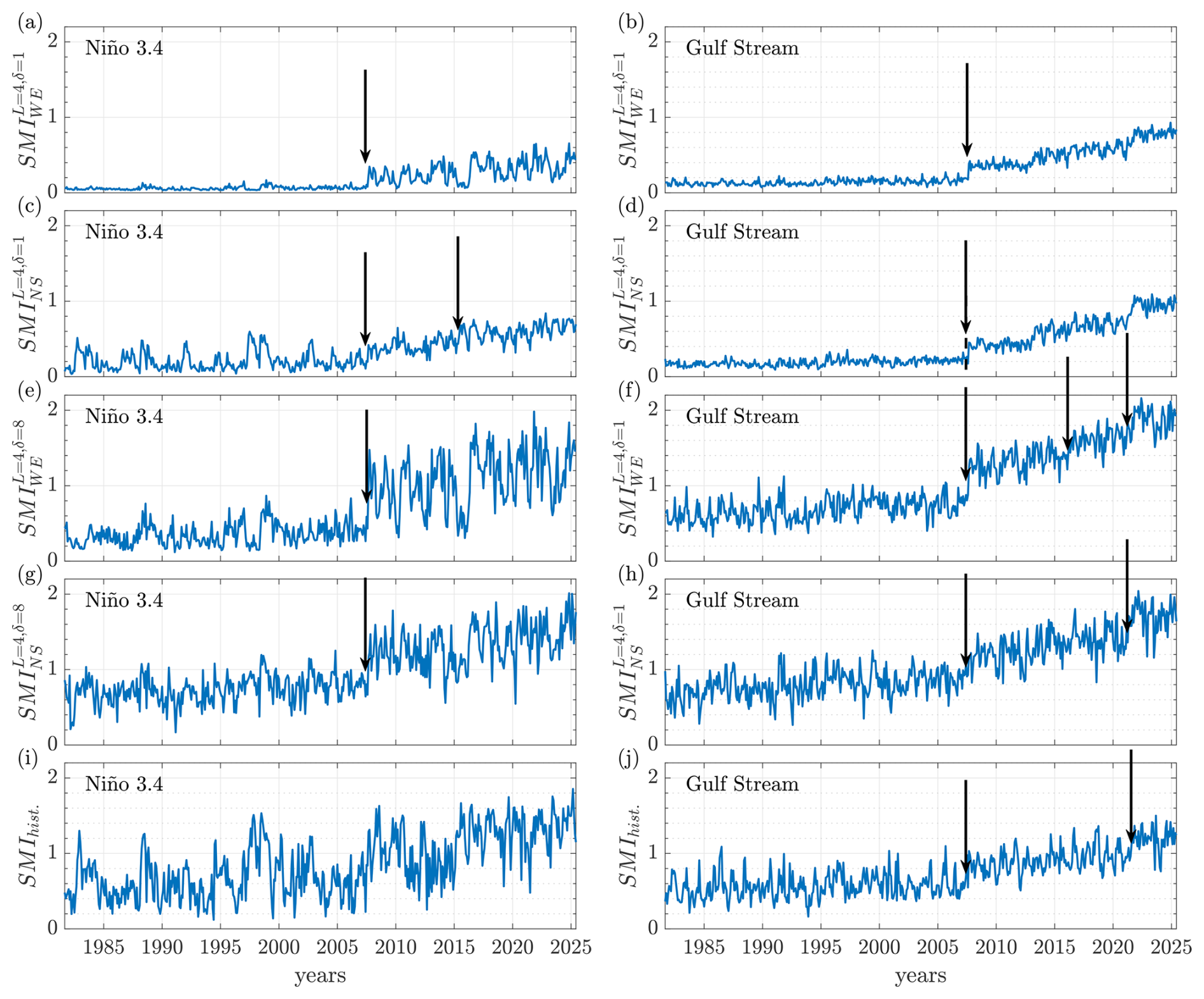
Figure 7 Spatial mutual information, Eq. (7), between SST anomalies of ERA5 and NOAA datasets. The left column corresponds to the Niño 3.4 region, while the right column, to the Gulf Stream region. In the first three rows, panels (a)–(h), SMI is calculated from the probabilities of ordinal patterns with δ=1 (a–d) and δ=8 (e–h); the OPs are constructed with WE orientation in (a), (b), (e), and (f), and with NS orientation in (c), (d), (g), and (h). In the bottom row, panels (i) and (j), SMI is calculated from the probabilities of the data values, using the same number of bins, 24, as the number of possible OPs. In all cases SMI increases with time, revealing, as expected, that the discrepancies between ERA5 and NOAA datasets diminish; however, note the difference in the vertical scales in (a–d) and (e–h): The higher SMI values when ordinal patterns are defined with a spatial lag δ=8 relative to δ=1 reveal that the agreement between the two data sets is better at long spatial scales than at short ones. The arrows indicate change points detected by the PELT algorithm.

For the Gulf Stream region (Fig. 7b, d, f, h, and j), all the SMI values reported present oscillations around a relatively constant value before 2007, which appears to increase consistently from this year on. Additionally, on the large scale, we detected two other transitions: one at end of 2015/beginning 2016 (the same observed in SMI_NS for δ=1 in the Niño 3.4 region), and another one in 2021. Both transitions correlate with changes in the satellites experienced by NOAA SST those years (Huang et al., 2023). We also note that 2016 corresponds to the start date of version 2.1 of the NOAA OI product, which also includes the Argo observational data (Huang et al., 2021), and several changes in the conventional and radiance observations assimilated by ERA5 also occurred that year (Hersbach et al., 2020).

Regarding SMI_hist., we observe that the annual cycle has some impact on this signal, but not on SMI_NS, nor SMI_WE.

Finally, to demonstrate the added value of using symbolic ordinal analysis, in Fig. 8 we present the results obtained with two well-known measures of linear relationship between two datasets: the average absolute difference, AAD, and the spatial Pearson's correlation coefficient, r. They provide complementary information because when AAD and r are both high, the data sets differ in values but their spatial distributions are consistent, whereas when both are low, there is agreement between the values, but not in the spatial distributions. In Fig. 8 we see that both measures show continuous improvement of the agreement between the two datasets in the two regions; however, there are oscillations and no clear transitions are observed. In the Gulf Stream region, AAD and r show a strong coupling with the annual cycle, with disagreement (high AAD and low r) peaking during northern winters. A possible explanation could be due to the high cloud coverage in this region during winters, which could difficult infrared measurements, leading to larger differences between ERA5 and NOAA datasets. On the other hand, in the Niño 3.4 region ENSO events affect the agreement between the datasets, but their effect is captured differently by the two measures. For example, AAD peaks during El Niño in 1988, 1997 and during La Niña of 2011, but these events do not affect r, and vice-versa, La Niña in 1996 and 1999, and El Niño in 2004, affect r but not AAD.

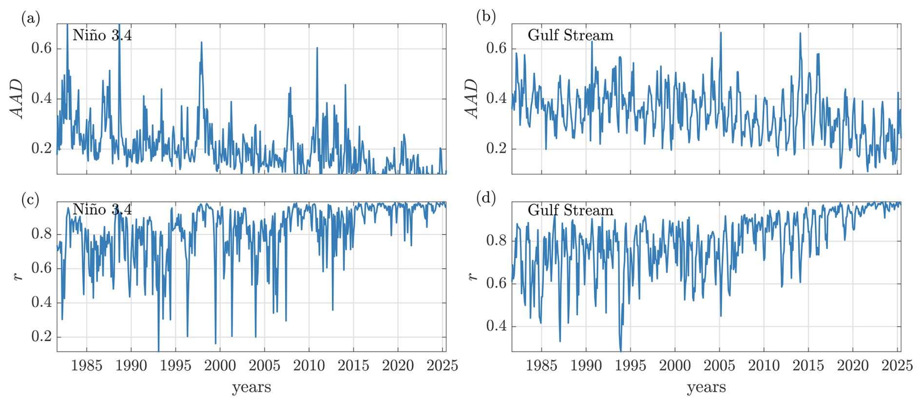
Figure 8 Average absolute difference, AAD (a, b), and spatial Pearson's correlation coefficient, r (c, d), between ERA5 and NOAA datasets in (a), (c) Niño 3.4 region, and (b), (d) Gulf Stream region.

For the same levels of statistical significance (with respect to surrogate data) and robustness (with respect to variations of the penalty parameter) used for the analysis of SMI signals, no robust and significant change points are detected in the analysis of AAD and r signals.

5 Conclusions

We have shown that a nonlinear quantifier, the spatial permutation entropy (SPE), is useful and flexible for analyzing the spatiotemporal dynamics of SST anomalies. SPE is computed from the probabilities of symbols, known as ordinal patterns (OPs), defined by four SST anomaly values in grid points that are geographically oriented north-south (NS) or west-east (WE), and that are separated by a spatial lag, δ: δ=1 corresponds to neighboring grid points separated by 0.25°; δ=8, to grid points separated by 2°.

We used the temporal variations of SPE calculated with NS or WE OPs, $H_{\text{NS}}^{L,\mathit{\delta }}$ and $H_{\text{WE}}^{L,\mathit{\delta }}$ respectively, to compare ERA5 and NOAA OI v2 SST anomalies in two key regions: Niño 3.4 and the Gulf Stream. By tuning the spatial lag δ, we were able to tune the spatial scale at which the datasets were compared.

A main conclusion of our study is that, in both regions, we found differences in the temporal evolution of $H_{\text{NS}}^{L,\mathit{\delta }}$ and $H_{\text{WE}}^{L,\mathit{\delta }}$ computed at short spatial scales, that is, using OPs made of neighboring points (Fig. 3). Differences gradually disappear when δ increases (Fig. 6), and when δ is large enough, the temporal variations of H_NS and H_WE in the two datasets are remarkably similar (Fig. 4). The short-scale differences found here between ERA5 and NOAA datasets by using SPE analysis add on to previously reported discrepancies (Yao et al., 2021; Dai, 2023). Importantly, our analysis also reveals clear improvements in the similarity of the two datasets in recent years, following significant advances in Earth observation systems due to the introduction of new satellite observations and new data processing methodologies.

Regarding these recent advances, they generated subtle changes in both datasets, and some of them were detected by our analysis technique. Specifically, the temporal variations of H_NS and H_WE allowed us to identify four transitions that occurred in 2007 when ERA5 changed its sea–surface boundary condition to OSTIA, in 2013 when OSTIA updated the background error covariances, in 2016 when several changes occurred both in NOAA (as the inclusion of MeteOp-B and Argo data) and ERA5, and in 2021 when NOAA SST changed satellite observations from MeteOp-A/-B to MeteOp-C. While these transitions can be observed by simply inspecting the temporal evolution of SPE, to corroborate these findings we applied an unsupervised change detection algorithm. Of course, not all the improvements in observation systems or data processing methodologies will modify the datasets in a way that can be detected by our analysis technique, therefore, methods that return complementary information should also be employed. Since the information lost by the SPE concerns the absolute values of the data, such methods should likely focus on that. Spatial Fourier analysis, or cross-correlation and mutual information analysis (Figs. 7 and 8), are all valid choices that can be used for a more complete dataset comparison.

We also report different temporal trends of $H_{\text{NS}}^{L=\mathrm{4},\mathit{\delta }=\mathrm{8}}$ and $H_{\text{WE}}^{L=\mathrm{4},\mathit{\delta }=\mathrm{8}}$ in the Niño 3.4 and Gulf Stream regions (Fig. 4) that are consistent in the two datasets. We interpret the different trends in terms of different responses to greenhouse gas forcing in the Niño 3.4 and Gulf Stream regions (uneven warming and cooling respectively).

In our study we calculated SPE from symbols in the NS and WE orientations only, which are particularly fit for the equatorial dynamics of the Niño 3.4 region. This region was selected because it is the one used to define ENSO events and captures the ocean-atmosphere interaction phenomena that characterize them. In contrast, for the Gulf Stream region the area analyzed was selected as a compromise to consider the Gulf Stream geographically (as the current moves away from the coast and flows northeast, it becomes the Gulf Stream extension or North Atlantic Drift) while also being the area with the strongest and relatively zonal currents. Even though this choice is a good approximation, given that the mean current's trajectory is not purely zonal, further work may consider other regions and orientations such as along current and across current. This would allow refining our results and better capturing latitudinal shifts. Additionally, we could integrate in the definition of the OPs not only the SST anomalies spatial variation (as done here) but also the temporal variation. This can be achieved by computing OPs in time, or by building the OPs in a way they extend both in space and time. The introduction of temporal OPs will allow us to integrate information from different time scales, since varying the value of δ allows us to study daily, intra-seasonal or interannual variations in SST anomalies. Moreover, the discrepancies, trends, and transitions found in this work can be confirmed and/or others can be uncovered, if different generalizations of ordinal analysis are used (for example, those that “weight” the symbols to include additional information from the signal Fadlallah et al., 2013).

Furthermore, it would be interesting to compare the results obtained with SPE and its temporal counterpart to those derived from linear analysis techniques, such as Fourier analysis. Since SPE relies on the relative ordering of data values, it constitutes a nonlinear approach, which we expect can yield results that complement those obtained by linear methods.

Finally, the increase in the spatial resolution of SST products seen in latest years will allow to investigate the role of the mesoscale and sub-mesoscale dynamics on bio-geo-chemical processes such as the importance of eddies and fronts on the distribution of nutrients, phytoplankton growth and carbon uptake. Thus, it is crucial that different SST products are able to characterize the small scale SST anomalies variability adequately. Our analysis reveals differences in SST datasets at these scales that could hinder their use. Additionally, with the emergence of AI climate emulators, ordinal analysis can be useful to compare AI models with traditional, physics-based ones.

Overall, our results highlight the versatility and robustness of SPE for analyzing the spatiotemporal dynamics of SST anomalies. Both the size and the orientation of the ordinal patterns play important roles in capturing the small scale differences between the datasets, and the long-term evolution in the analyzed regions. This evolution at the large scale is consistent with the consequences of global warming. Furthermore, SPE allows the identification of change points just by visual inspection, which could be traced back to specific changes in methodology and data inputs in the two SST products. Since not every modification of the SST products has consequences that can be detected by our analysis technique, we propose using ordinal analysis in conjunction with other linear or nonlinear methodologies, to obtain a more complete characterization of the dynamics.

Appendix A: Unsupervised CPD algorithm PELT

Table A1 Summary of the significant change points detected by the PELT algorithm. An asterisk next to the R value indicates that the change point is discussed in the main text.

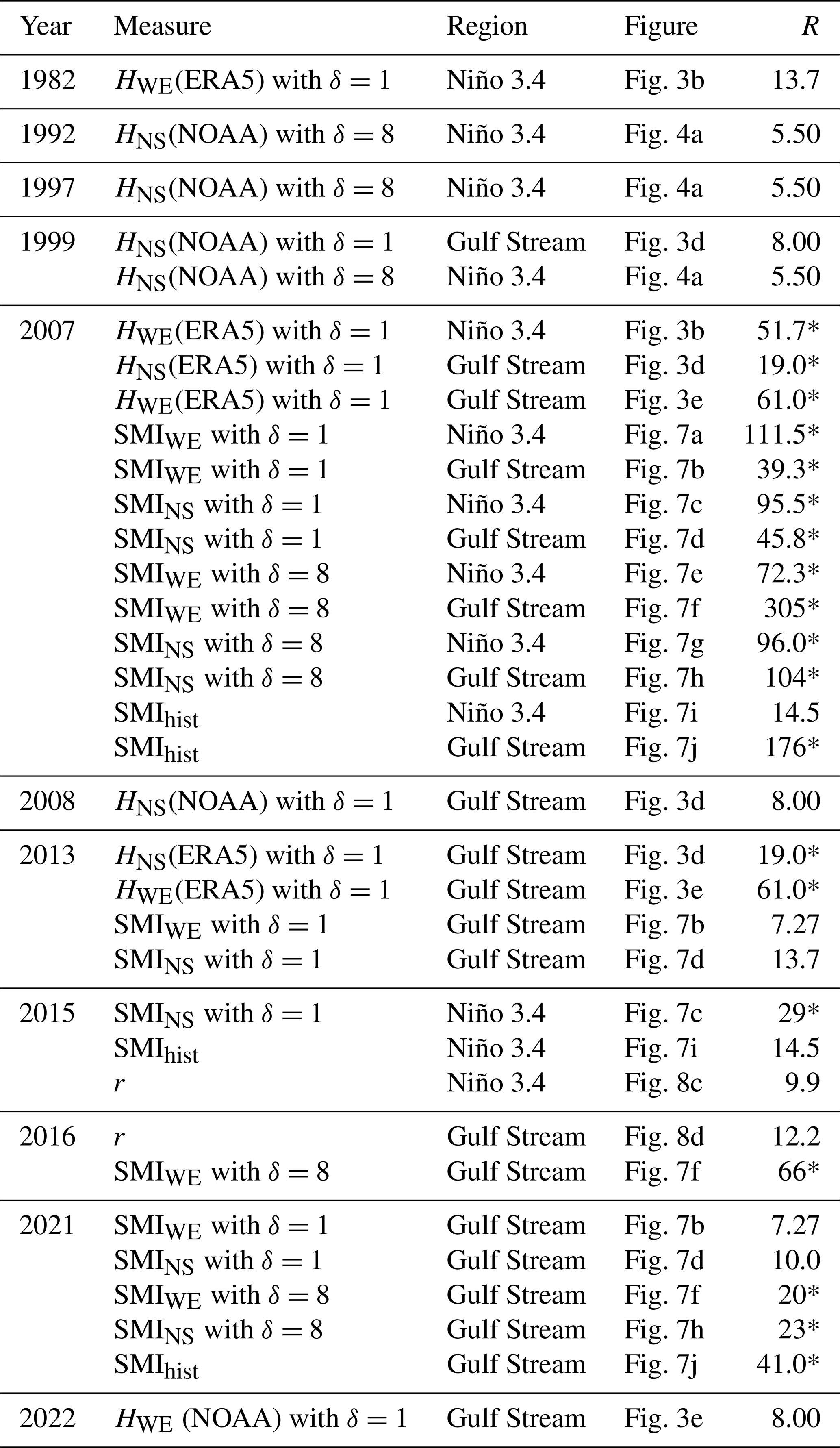
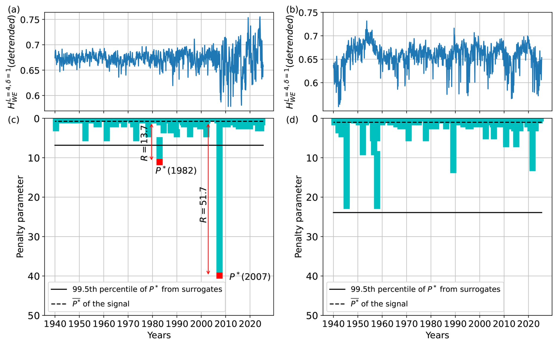
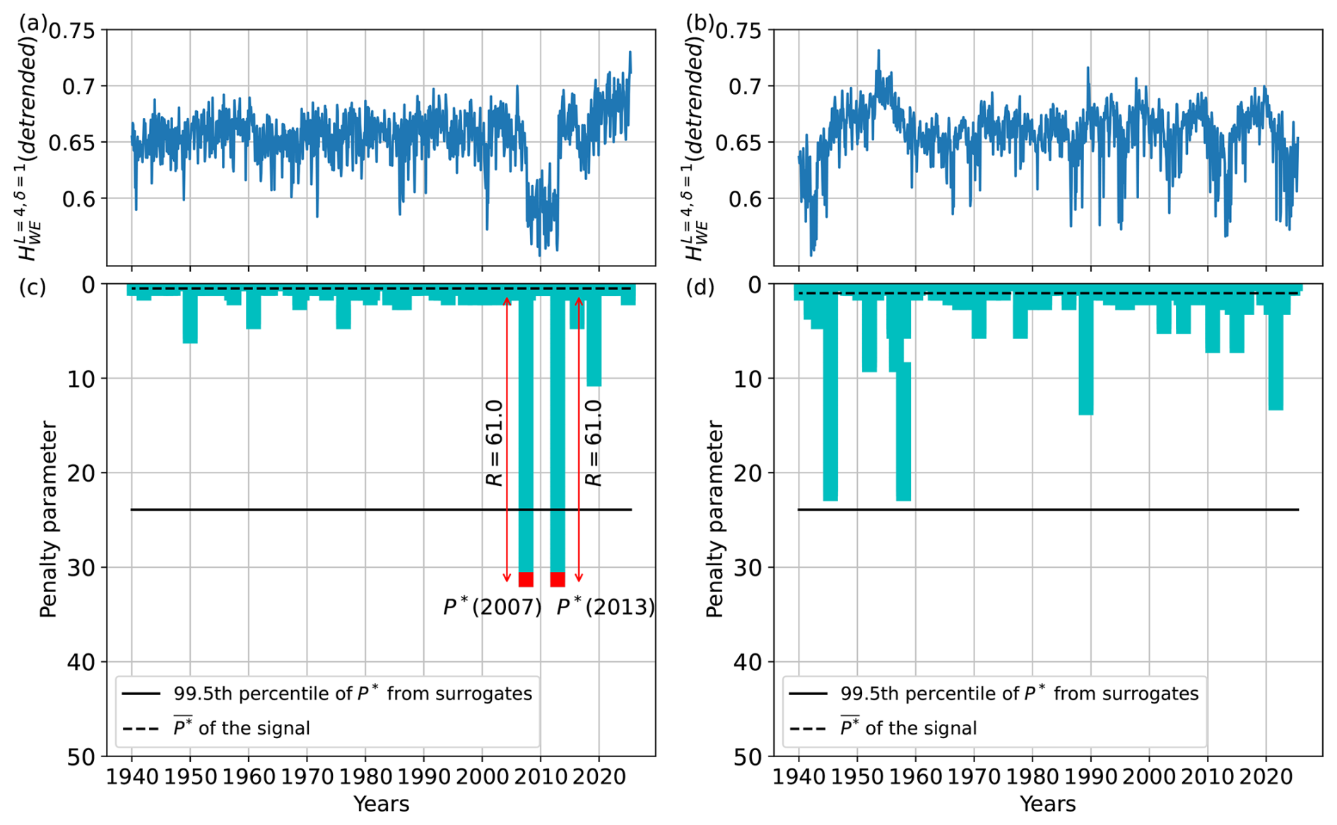
Figure A1 Robustness of the change points detected in the signal of H_WE from the ERA5 dataset with δ=1 in the Niño 3.4 region. Panel (a) shows the original signal detrended, while panel (b) shows its iAAFT surrogate (Schreiber and Schmitz, 1996). Panels (c) and (d) display the corresponding bar plots showing the persistence of each detected change point as the penalty parameter is increased. Dashed line corresponds to $\stackrel{\mathrm{‾}}{P^{*}}$ of the signal, while the continuous line marks the 99.5th percentile of P^* from the surrogates.

Figure A2 Same as Fig. A1, but for the Gulf Stream region.

A1 Implementation

To formally detect transitions in the quantities introduced in Sect. 3.1, we applied a CPD algorithm known as Pruned Exact Linear Time (PELT) (Killick et al., 2012) implemented in the Python package ruptures (Truong et al., 2020), with a Gaussian kernel cost function. PELT has been used to analyze geophysical time series such as temperature (Khapalova et al., 2018), vegetation (Wang and Fan, 2021), and stream flow (Rocha and de Souza Filho, 2020). Given a penalty parameter, P, PELT returns a number of change points. The value of P needs to be carefully selected because it determines the number of change points found: if it is too low, too many change points are detected, while if it is too high, no change point is detected. To deal with this problem, we propose a methodology similar to changepoints for a range of penalties – CROPS (Haynes et al., 2017). As in CROPS, we evaluate a large range of penalty parameters. However, CROPS ultimately relies on manually choosing the optimal penalty value (usually graphically) for which perturbations of its value do not alter significantly the number of change points detected. Our approach is intended to avoid this kind of subjectivity in the implementation, providing clear and quantifiable criterion for the selection of the penalty value, while at the same time selecting the most significant change points, as an attempt to minimize false detections. The procedure followed to select P is based on two steps: the first consists of the analysis of surrogate time series where the null hypothesis (NH) is that there are no change points, and the second step is the analysis of the robustness of the change points passing the surrogate test, with respect to variations in the penalty parameter. However, we note that NH can sometimes fail and surrogate signals still present change points that are detected by PELT at high values of P, and therefore the selected significance threshold may be too high, which can result in genuine change points not being detected, even if they are visually evident. Therefore, while PELT is a helpful method for change point detection, it should be further refined in future work.

CPD analysis typically assumes that the signals are piecewise stationary (Truong et al., 2020), and that within each segment the distribution follows an independent and identically distributed sequence of random variables (Garreau and Arlot, 2018), therefore linear trends have to be removed before using the PELT algorithm. This was the case for the time series of the spatial permutation entropy (Eq. 1), and of the linear measures (AAD and r), where a simple detrend was sufficient as pre-processing. In contrast, for the time series of the spatial mutual information (Eq. 7), sections with and without a linear trend are observed in the signal; hence we performed the following sequence of steps: (1) The time series were first divided in segments where the linear trend is constant. To do this, we combined the PELT algorithm with a statistical test of the linear trend: we run PELT without detrending the input, and test if there is a significant (p value<0.01) linear trend using a Wald test. If two continuous sections fail the test (i.e. none of them has a linear trend) or they have different results of the test (i.e. one has a significant linear trend while the other has not), the change point is considered as a true, genuine change-point. Otherwise, the change-point was disregarded as an artifact due to the linear trend present. (2) After performing this procedure for every change-point discovered by the first iteration of PELT, we detrend the signal in each segment delimited by the genuine change-points, and (3) Run the PELT again in each of these segments to detect change points in them. In these signals, no change points were detected within these detrended segments, but all reported ones correspond to transitions between in the linear trend/no trend, with significance assigned by the Wald test (Step 1), so there was no need to compute the surrogates of these signals.

For the other signals, the ones with a single trend (SPE, AAD, and r), in order to select an appropriate value of P, the following procedure was performed: (1) Each signal was detrended. (2) 10 iterated Amplitude Adjusted Fourier Transform (iAAFT) surrogates (Schreiber and Schmitz, 1996) were generated for each signal. (3) Each surrogate was analyzed in a range of $P\in [\mathrm{1},\mathrm{50}]$. (4) For each change point detected (between 400–600 total in the 10 surrogated signals), we recorded the maximum P for which it is detected (from now on we note this value by P^*). (5) The 99.5th percentile of this distribution of P^* is selected as the value of P for which we analyze the original detrended signal.

In the previous step we have identified significant change points by comparing changes in the signal with changes in the surrogates generated from the signal. Now we test if these change points are robust in the sense that they can be detected for penalty values considerably higher than the median of change points (including not significant). For this, we first calculate the maximum penalty parameter for which each change point is detected, P^*, and then calculate the relative difference between P^*(t) of the significant change point that occurs at time t and the median of P^* for all the change points detected in the signal ($\stackrel{\mathrm{‾}}{P^{*}}$):

$$\begin{array}{}\text{(A1)}& {\displaystyle }{\displaystyle }R\left(t\right)={\displaystyle \frac{P^{*}\left(t\right)-\stackrel{\mathrm{‾}}{P^{*}}}{\stackrel{\mathrm{‾}}{P^{*}}}}.\end{array}$$

Some change points have a relatively low robustness score, and they are significant in the sense that the surrogate time series did not display almost any change points. To avoid this effect, in the main text we have only shown change points with a robustness score R≥19, which discards the first two quartiles of the distribution of R values, but in Table A1 we include all the significant change points and their corresponding R values.

Now, in Fig. A1c, we show an example of such analysis performed in the signal of H_WE from the ERA5 dataset with δ=1 in the Niño 3.4 region (blue signal in Fig. 3a). Here we show the change points detected as a function of the penalty parameter, P, in cyan. In black continuous line, we mark the 99.5th percentile of the distribution of maximum P for which each change point is detected, P^*, in the surrogated signals. In black dashed line, we display the median of P^* from the signal: $\stackrel{\mathrm{‾}}{P^{*}}$. In red we have highlighted the P^* of the two significant change points (those which can be detected for P larger than the 95th percentile of P^* from the surrogated signals), but only one (in 2007) is robust enough (the relative distance, R, between P^* and $\stackrel{\mathrm{‾}}{P^{*}}$ is larger than 19) to be considered a true change point.

Panel (b) of Fig. A1 showcases an example of an iteratively adjusted amplitude adjusted Fourier transform (IAAFT) surrogate (Schreiber and Schmitz, 1996) obtained from the signal from panel (a), and panel (d) show the results of the Pelt algorithm for different penalty parameters.

Figure A2 displays the same analysis, but now for the Gulf Stream region. In the case of this signal, the surrogates produce change points that are quite robust (see Fig. A2d) which increases the significance threshold (black continuous line) considerably. However, two significant change points are detected, which are also robust.

A2 Summary of detected points

Table A1 summarizes the significant change points returned by the PELT algorithm. Here we can see how the 2007 transition is widely detected by different ordinal measures (H and SMI), in both regions and mainly on the small scale (δ=1). However, the other transitions, specifically the ones in 2013 and 2021, are only detected in the Gulf Stream region. Additionally, it is clear that the majority of the transitions are only detected by SMI, computed from ordinal pattern probabilities.

The signals of SMI shown in Fig. 7, especially those obtained from ordinal patterns (panels a–h), present sections with and without a linear trend, most notably pre- and post-2007. All the change points found on the small scale (Fig. 7a–d) correspond to a transition between the signal having a significant nonzero linear trend and a nonsignificant linear trend (or vice versa). On the other hand, the 2007 change point at the large scale (Fig. 7e–h) always present a linear trend before and after this year, but these change point persist after detrending the signal. Regarding the other change points detected at the large scale in the Gulf Stream region, the one in 2016 in SMI_WE and the one in 2021 in SMI_NS correspond again to transitions trend/no-trend, while the one in 2021 in SMI_WE corresponds to a jump: no significant linear trend before or after.

For SMI_hist. in the Gulf Stream region region (Fig. 7j, the algorithm detects two change points, but one in 2007 and the other one in 2021. The first one corresponds to a change point with linear trend before and after, which survives detrending, and the second one corresponds to a trend/no-trend transition.

In addition to the suitability of the chosen surrogates mentioned before (change points still occur in the surrogates, which increases the significance threshold and prevents the detections of true change points), we highlight that the last step in our CPD analysis, the robustness check of the significant change points, allowed us to distinguish between what look like spurious detections and evident ones (such as 2007). But some of the discarded change points (as in 2013 or 2021 in SMI_WE and SMI_NS for δ=1 in the Gulf region), which are visually evident and significant, do not present large robustness levels. In fact, although the relative robustness (R) is computed from each signal, the threshold for significant robustness ($\stackrel{\mathrm{‾}}{R}$) is computed from the robustness distribution obtained by considering all the robustness values from all the change points detected in all the time series (entropies, mutual information, and linear measures). Therefore, the robustness values of a single time series affect the robustness threshold by affecting the median of the distribution. For example, a time series with many robust change points (high P) would increase the median of P, making R small and the robustness of its own change points less significant; or a time series with a single very robust change points (high R) increases the overall median of R ($\stackrel{\mathrm{‾}}{R}$) potentially making non-significant robust change points of another time series. However, the change points that pass the double check of significance and significant robustness are simultaneously robust to other change points in the signals and to all other significant change points.

While ordinal analysis allows us to detect several changes that could not be detected by the distance or cross-correlation measures considered, it has the drawback that ordinal analysis typically has computational costs and hyper-parameters (the length of the symbol and the lag) which need to be carefully selected. However, ordinal analysis has the important advantage of offering a large degree of flexibility, by allowing to tune the shape of the pattern, and the spatial scale of the analysis.

Appendix B: Supporting information

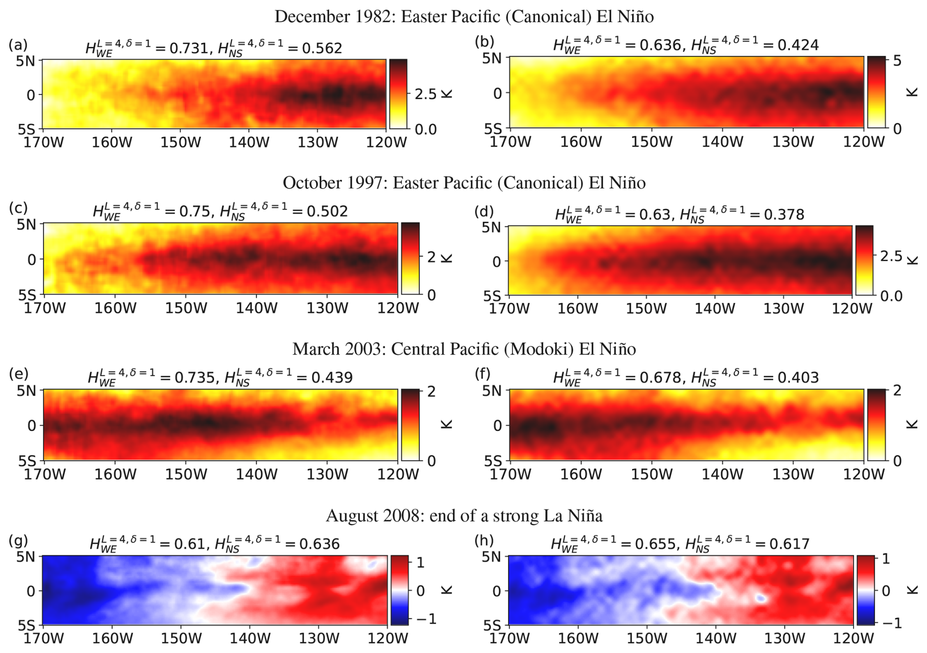
Figure B1 Snapshot of the Niño 3.4 region SST anomalies during different El Niño/La Niña events from NOAA (left column) and ERA5 (right column) datasets.

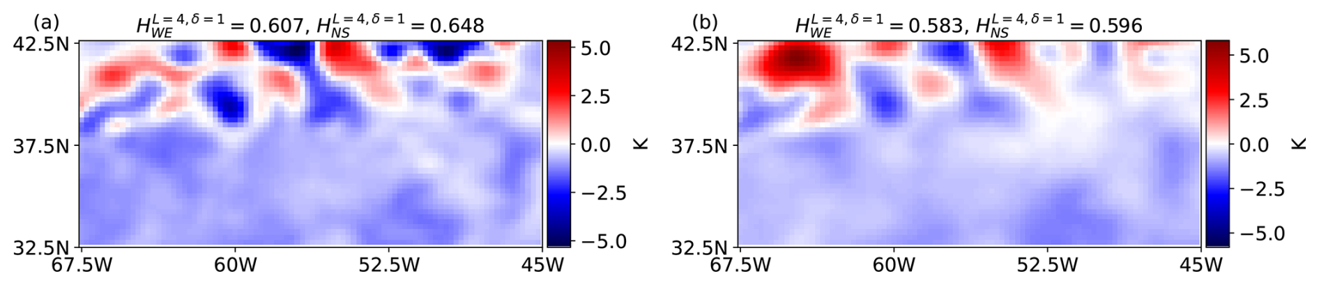
Figure B2 Snapshot of the Gulf Stream region during a large meandering in January 2010 (Zeng and He, 2016) from NOAA (left column) and ERA5 (right column) datasets.

Figure B3 Same as Fig. 3 but for L=3.

Figure B4 Same as Fig. 3 but for L=5.

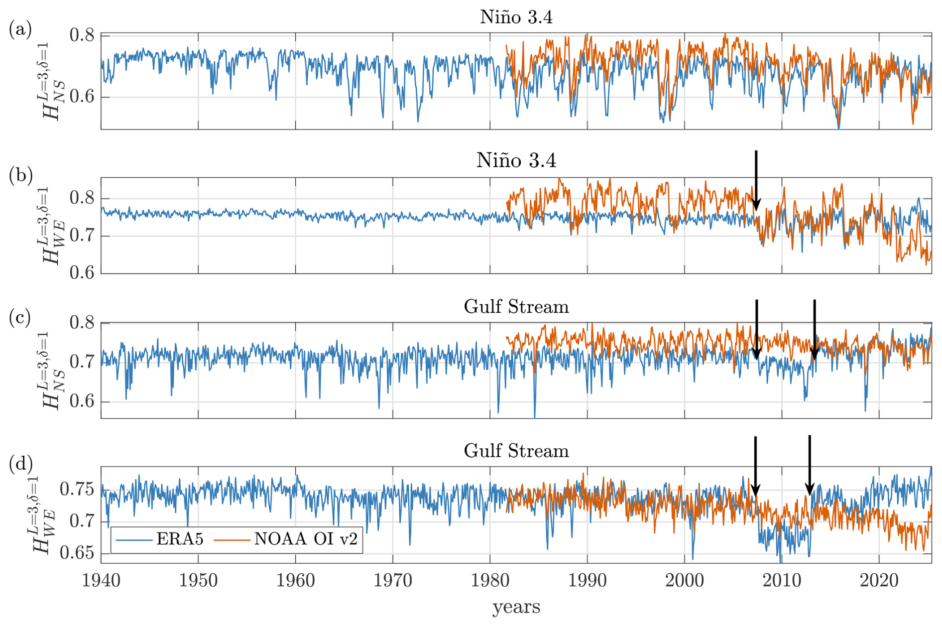
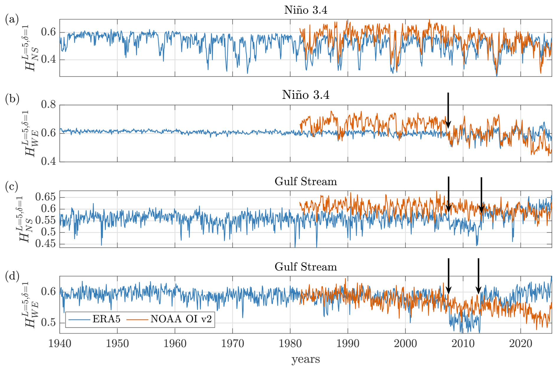
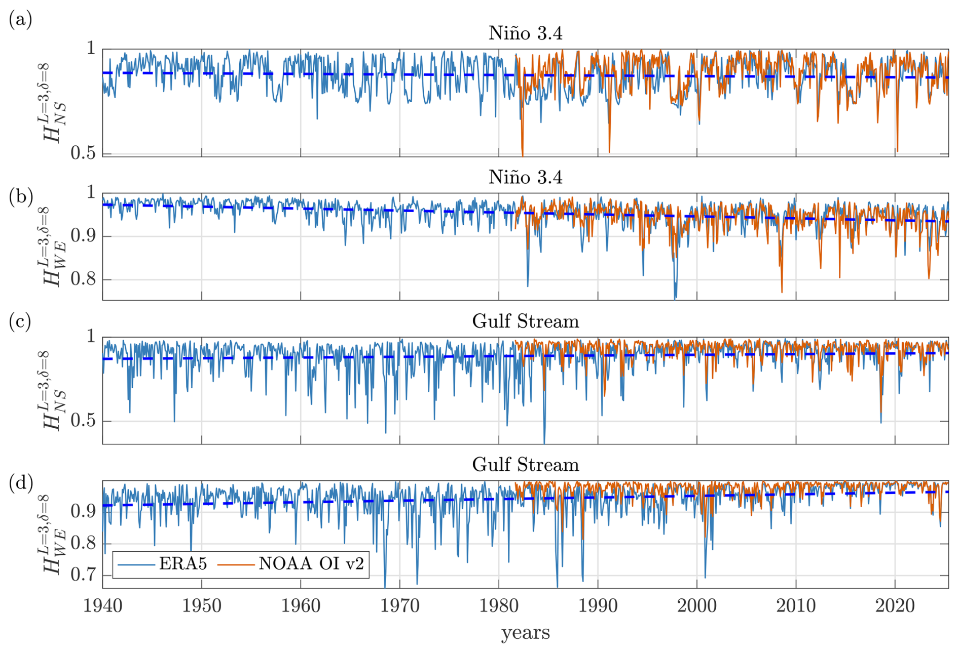
Figure B5 Same as Fig. 4 but for L=3. Fittings of the ERA5 data have a linear coefficient of: (a) $-\mathrm{2.28}{\mathrm{e}}^{-\mathrm{4}}{\text{yr}}^{-\mathrm{1}}$ ($p\text{ value}=\mathrm{3.4}{\mathrm{e}}^{-\mathrm{1}}$), (b) $-\mathrm{4.20}{\mathrm{e}}^{-\mathrm{4}}{\text{yr}}^{-\mathrm{1}}$ ($p\text{ value}=\mathrm{1.0}{\mathrm{e}}^{-\mathrm{9}}$), (c) $\mathrm{5.52}{\mathrm{e}}^{-\mathrm{4}}{\text{yr}}^{-\mathrm{1}}$ ($p\text{ value}=\mathrm{9.6}{\mathrm{e}}^{-\mathrm{3}}$), (d) $\mathrm{5.04}{\mathrm{e}}^{-\mathrm{4}}{\text{yr}}^{-\mathrm{1}}$ ($p\text{ value}=\mathrm{2.2}{\mathrm{e}}^{-\mathrm{6}}$).

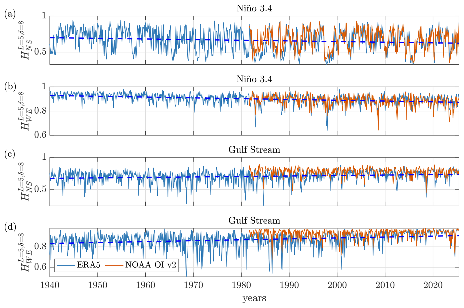
Figure B6 Same as Fig. 4 but for L=5. Fittings of the ERA5 data have a linear coefficient of: (a) $-\mathrm{8.16}{\mathrm{e}}^{-\mathrm{4}}{\text{yr}}^{-\mathrm{1}}$ (p value=0.087), (b) $-\mathrm{6.00}{\mathrm{e}}^{-\mathrm{4}}{\text{yr}}^{-\mathrm{1}}$ ($p\text{ value}=\mathrm{8.0}{\mathrm{e}}^{-\mathrm{10}}$), (c) $\mathrm{9.00}{\mathrm{e}}^{-\mathrm{4}}{\text{yr}}^{-\mathrm{1}}$ ($p\text{ value}=\mathrm{1.0}{\mathrm{e}}^{-\mathrm{5}}$), (d) $\mathrm{8.88}{\mathrm{e}}^{-\mathrm{4}}{\text{yr}}^{-\mathrm{1}}$ ($p\text{ value}=\mathrm{1.4}{\mathrm{e}}^{-\mathrm{8}}$).

Figure B7 Same as Fig. 7 of the main text but for L=3 (and 6 bins for SMI_hist.).

Figure B8 Same as Fig. 5 but for the Gulf Stream regions. The Pearson correlation coefficients between the mean SST anomaly and the entropy signals are shown in Table 2.

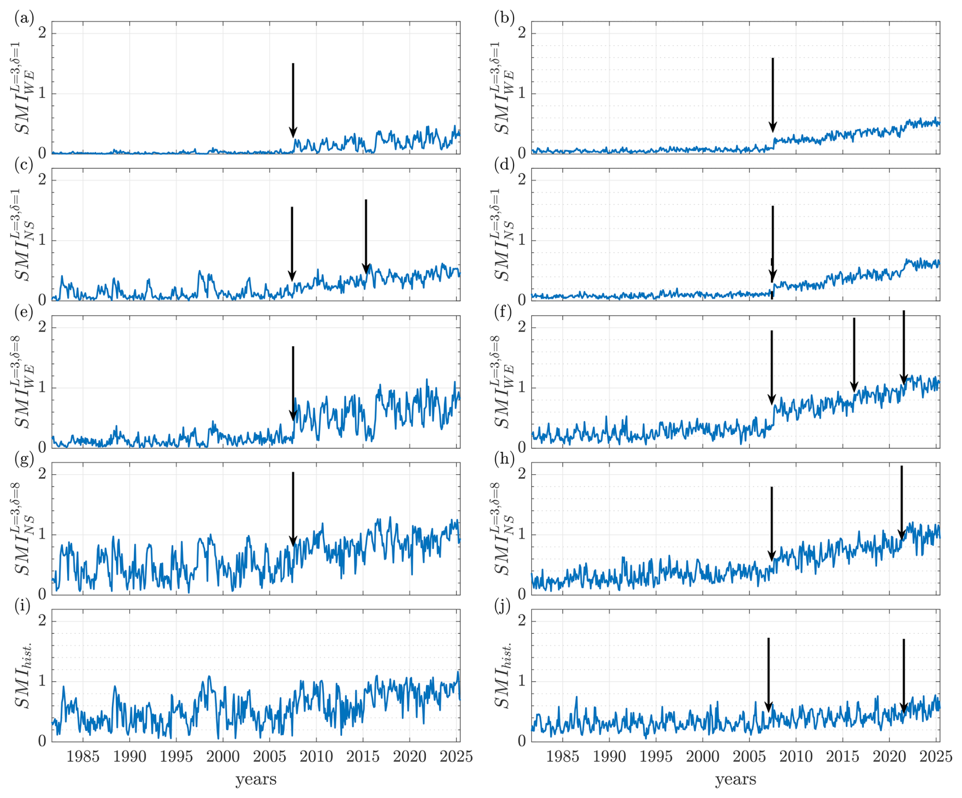
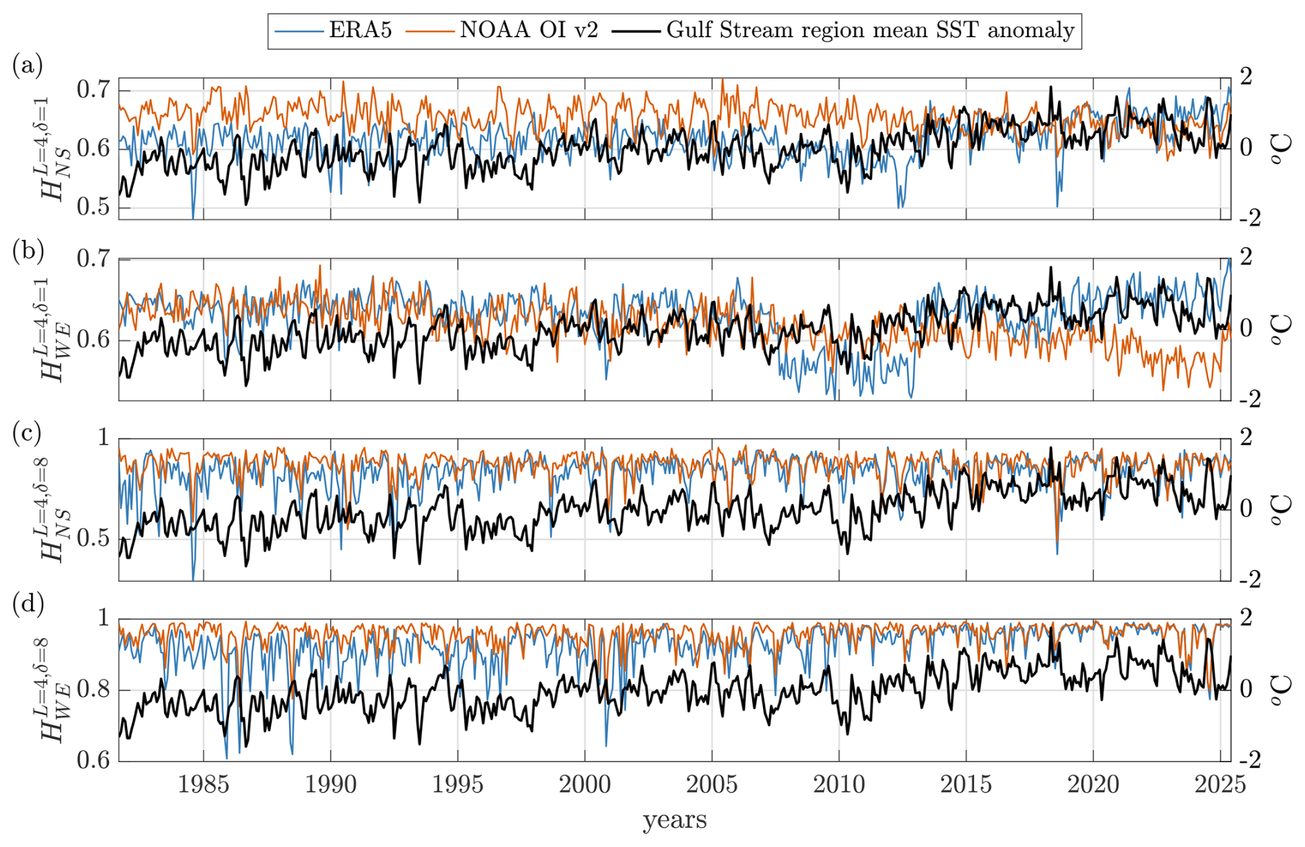
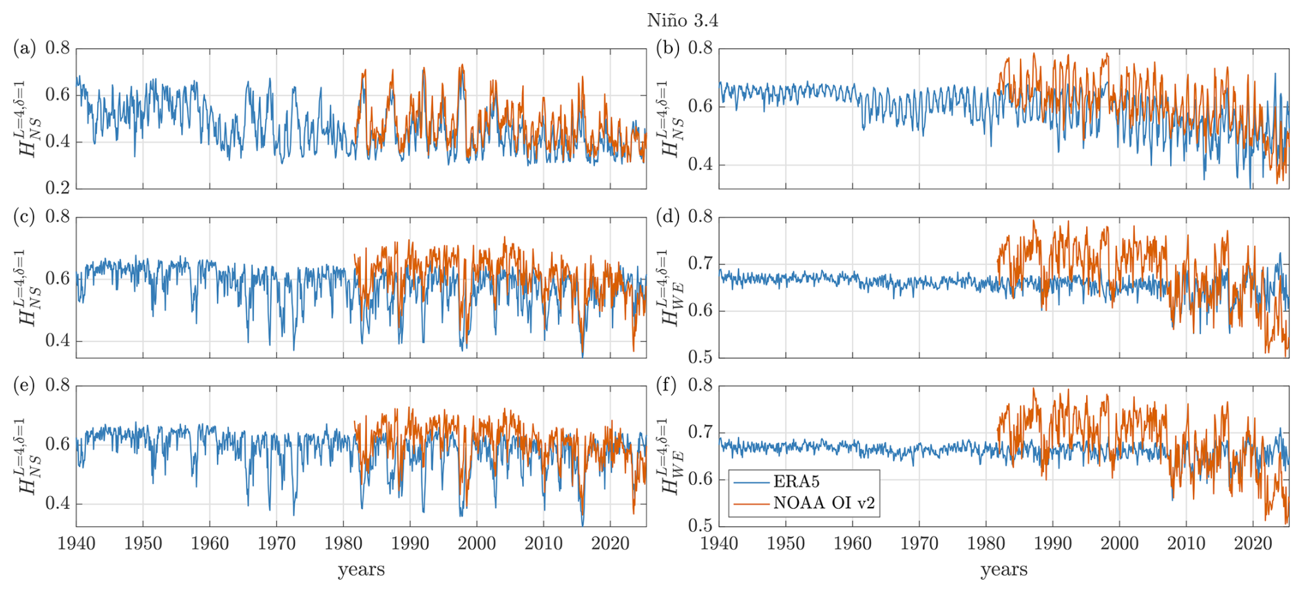
Figure B9 Analysis of the Niño 3.4 region, with L=4 and a small spatial lag (δ=1) of the raw data (top row), of the anomalies (after removing the seasonal cycle, as in the manuscript, middle row) and of the detrended anomalies (after removing the linear trend and the seasonal cycle, bottom row). The columns display results for the two OP orientations (left: NS; right: WE).

Figure B10 Same as Fig. B9 but for δ=8.

Figure B11 Same as Fig. B9 but for the Gulf Stream region.

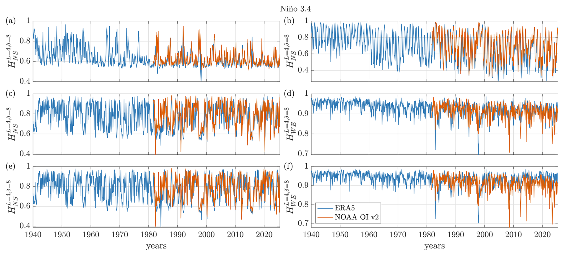
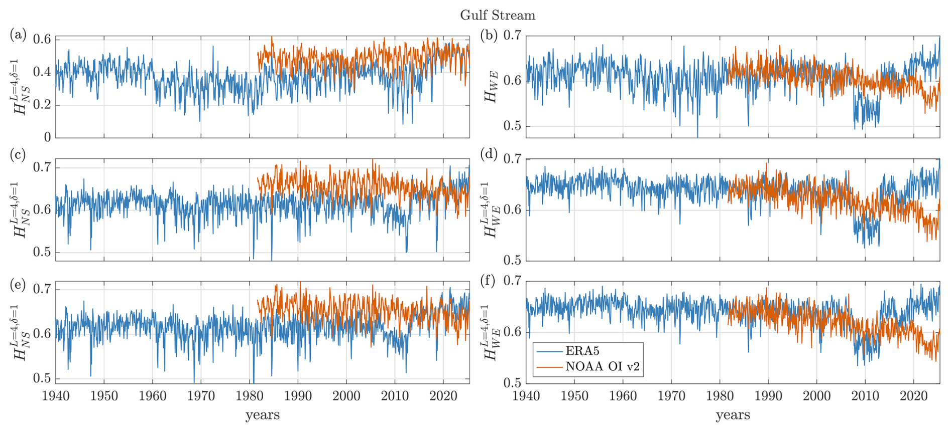
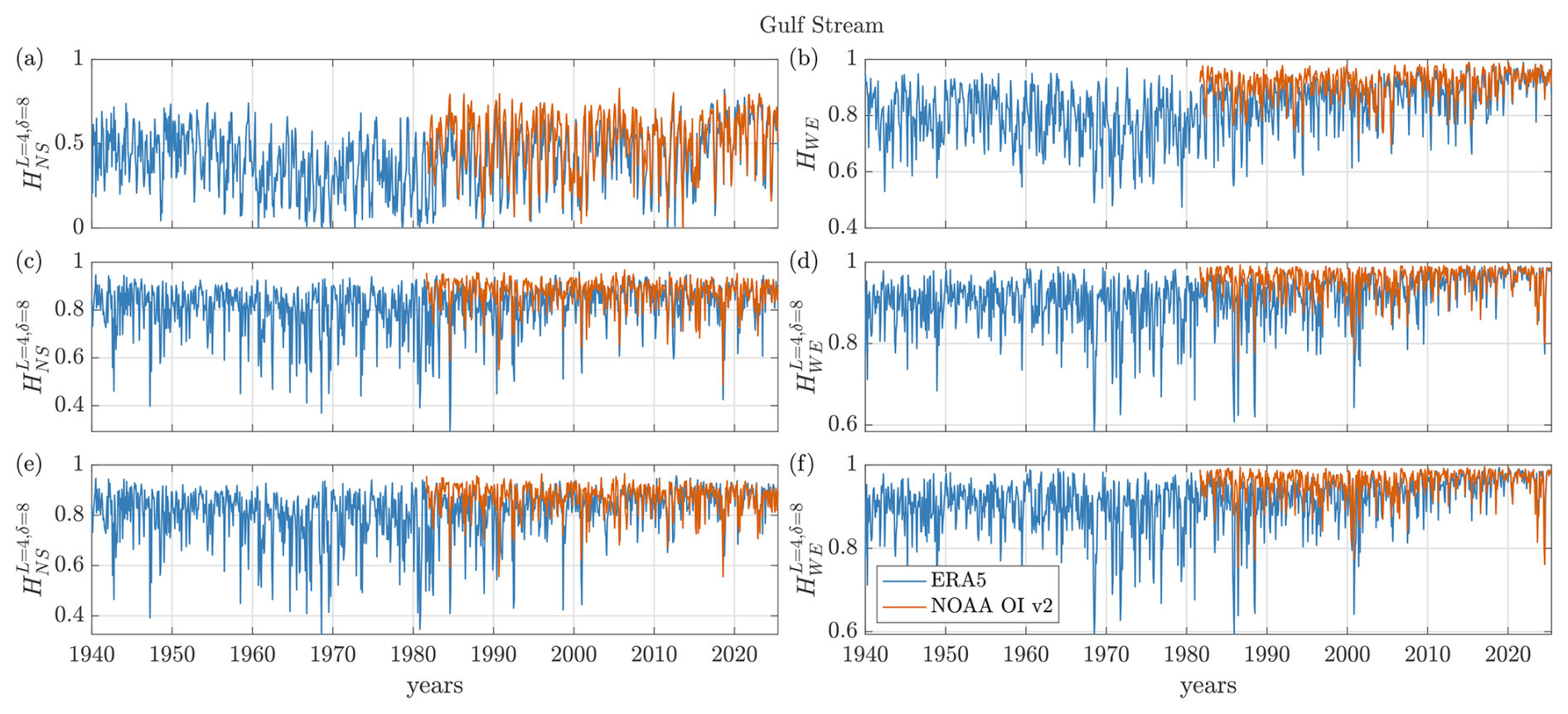
Figure B12 Same as Fig. B11 but for δ=8. The variation of the entropies in the top row of Figs. B9 and B10 is consistent with the fact that in the equatorial Pacific, the seasonal cycle is significant in the WE direction and therefore manifests itself on both short and long scales. In the Gulf Stream, Figs. B11 and B12, the seasonal cycle is more significant in the NS direction because the current is nearly zonal. Therefore, it can be seen in NS when using δ=1 (panel a in Fig. B11), but not in the WE direction (panel b in Fig. B11). However, when δ=8, the distances are large enough for the seasonal cycle to also manifest itself also in the WE direction (panel b in Fig. B12).

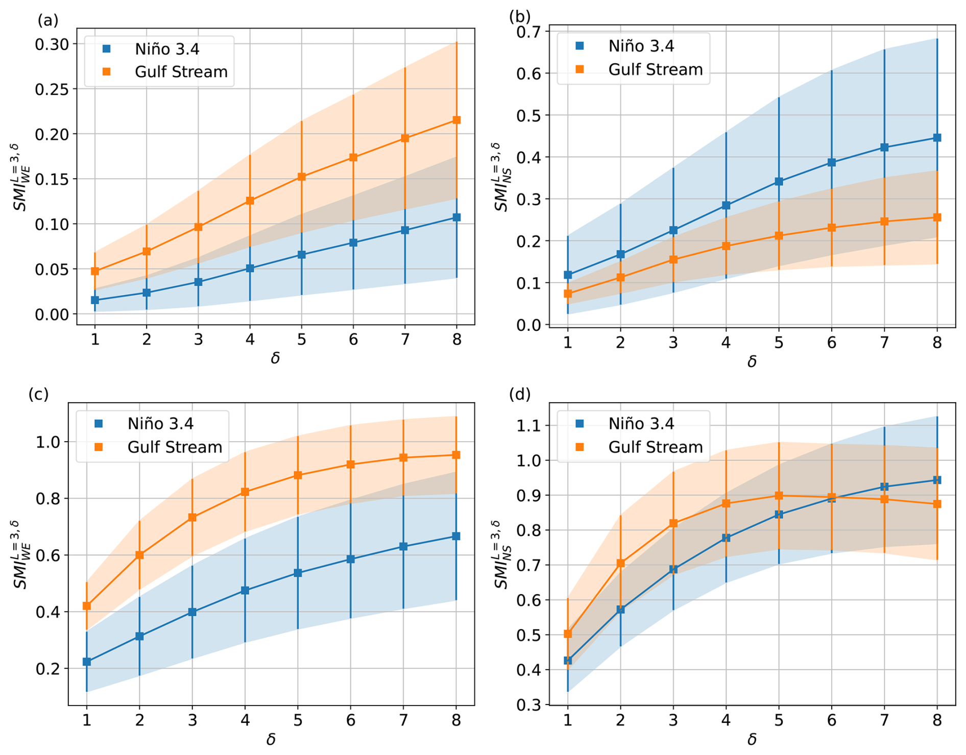
Figure B13 Spatial Mutual Information (SMI^L,δ) as a function of the spatial lag, δ, in the two regions considered, and for the two orientations of the ordinal patterns (WE and NS). The analysis was done for the first 120 months (top row) and for the last 120 months (bottom row) of the time interval in which both, ERA5 and NOAA OI v2 datasets are available (1981–2025). The symbols show the mean value and the error bars show the standard deviation. Here we show analysis for ordinal patterns of length L=3, but similar results were obtained with L=4 (see Fig. B14). Note the different vertical scales. Here we see that the agreement between the datasets improves with δ, and, for the same δ, the similarity between the two datasets in the two periods is quite different, being more similar in the second period (note the different vertical scale). In general, the two datasets are more similar in the Gulf than in the Pacific, which can be due to the fact that the North Atlantic is the area with the highest concentration of in-situ measurements globally. In the Gulf Stream region, the similarity of the two datasets for the NS orientation saturates for δ=5, that is, when the NS ordinal patterns cover 4°, meaning the submesoscale (0.1–10°), an intermediate scale between typical ocean turbulence and eddies. In contrast, in the case of the Niño 3.4, there does not appear to be a scale at which the similarity of the datasets stops increasing.

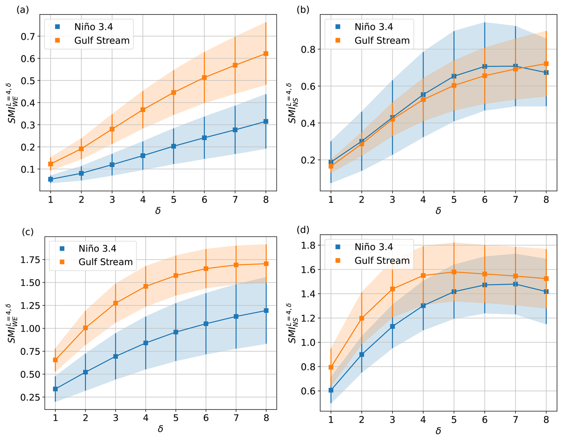
Figure B14 Same as Fig. B13 but for L=4. Similar results are obtained, only that ${\text{SMI}}_{\text{NS}}^{L=\mathrm{4},\mathit{\delta }}$ saturates for δ=6 in the Niño 3.4 region.

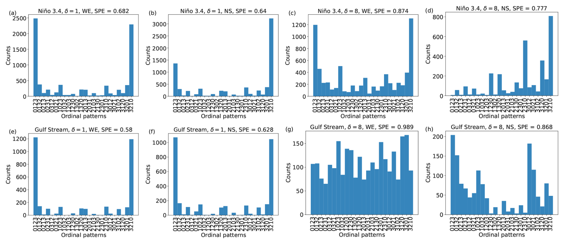
Figure B15 Ordinal probabilities in the Niño 3.4 region (top row) and in the Gulf Stream region (bottom row) calculated from NOAA for January 2015) with δ=1 (a, b, e, f) and with δ=8 (c, d, g, h). The value of the spatial permutation entropy is indicated in each panel.

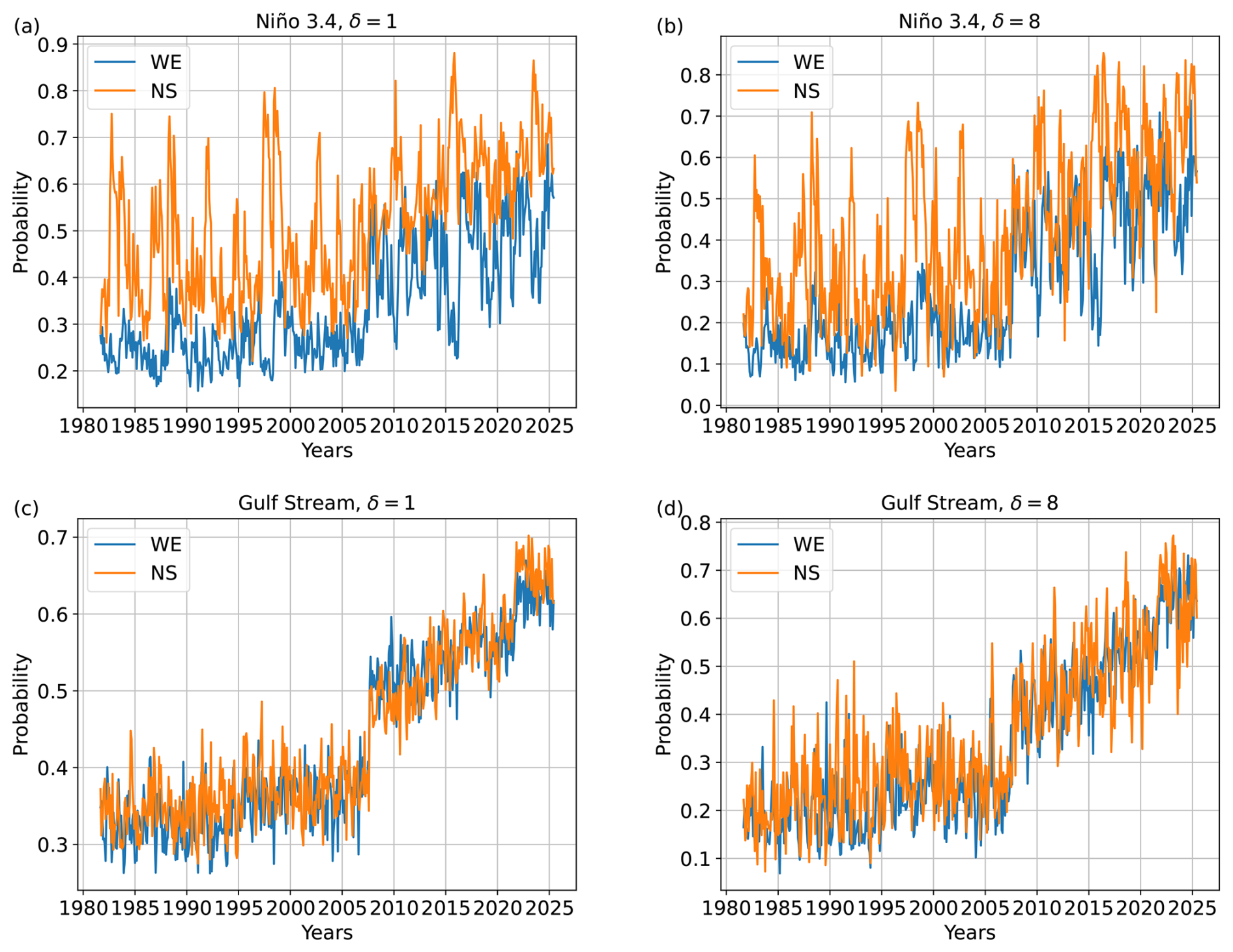
Figure B16 Evolution of the probability that, in a grid point the spatial ordinal pattern (in the NS or WE direction) is the same in the two datasets. Panels (a) and (b) correspond to the Niño 3.4 region, while panels (c) and (d) to the Gulf Stream region. In panels (a) and (c) the ordinal patterns are constructed with δ=1, while in panels (b) and (d) with δ=8.